


1 Introduction
A fruitful approach to the study of geometric structures on a topological space X is to introduce a bounded numerical invariant whose maximum detects those structures on X which have many symmetries. An instance of this situation is the study of the representation space of lattices in (semi)simple Lie groups. More precisely, given two simple Lie groups of non-compact type $G,G'$
and a lattice
$G,G'$
and a lattice $\Gamma \leq G$
, Burger and Iozzi [Reference Burger and IozziBI09] described how to associate to every representation
$\Gamma \leq G$
, Burger and Iozzi [Reference Burger and IozziBI09] described how to associate to every representation $\rho \colon \Gamma \rightarrow G'$
a real number. Using the pullback map
$\rho \colon \Gamma \rightarrow G'$
a real number. Using the pullback map $\operatorname {\mathrm{H}}^{\bullet}_{cb}(\rho )$
induced by
$\operatorname {\mathrm{H}}^{\bullet}_{cb}(\rho )$
induced by $\rho $
in continuous bounded cohomology, they defined a numerical invariant
$\rho $
in continuous bounded cohomology, they defined a numerical invariant $\lambda (\rho )$
, which depends on a chosen class
$\lambda (\rho )$
, which depends on a chosen class $\Psi ' \in \operatorname {\mathrm{H}}^{\bullet}_{cb}(G';\operatorname {\mathrm {\mathbb {R}}})$
, as follows:
$\Psi ' \in \operatorname {\mathrm{H}}^{\bullet}_{cb}(G';\operatorname {\mathrm {\mathbb {R}}})$
, as follows:
 $$ \begin{align*}\lambda(\rho) := \langle \operatorname{\mathrm{comp}}^{\bullet}_\Gamma \circ \operatorname{\mathrm{H}}^{\bullet}_{cb}(\rho)(\Psi'), [\Gamma \backslash \operatorname{\mathrm{\mathcal{X}}}] \rangle, \end{align*} $$
where $\operatorname {\mathrm {comp}}^{\bullet}_\Gamma $
denotes the comparison map (§2.3),
$\operatorname {\mathrm {comp}}^{\bullet}_\Gamma $
denotes the comparison map (§2.3), $\operatorname {\mathrm {\mathcal {X}}}$
denotes the Riemannian symmetric space associated with G,
$\operatorname {\mathrm {\mathcal {X}}}$
denotes the Riemannian symmetric space associated with G, $[\Gamma \backslash \operatorname {\mathrm {\mathcal {X}}}]$
is the (relative) fundamental class of the quotient manifold, and
$[\Gamma \backslash \operatorname {\mathrm {\mathcal {X}}}]$
is the (relative) fundamental class of the quotient manifold, and $\langle \cdot , \cdot \rangle $
is the Kronecker product. We say that
$\langle \cdot , \cdot \rangle $
is the Kronecker product. We say that $\lambda (\rho )$
is a multiplicative constant if it appears in an integral formula, called a useful formula by Burger and Iozzi [Reference Burger and IozziBI09]. When
$\lambda (\rho )$
is a multiplicative constant if it appears in an integral formula, called a useful formula by Burger and Iozzi [Reference Burger and IozziBI09]. When $\lambda $
is a multiplicative constant, the formula implies that the numerical invariant has bounded absolute value. In several cases [Reference Bucher, Burger, Iozzi and PicardelloBBI13, Reference Bucher, Burger and IozziBBI18, Reference PozzettiPoz15], its maximum corresponds precisely to representations induced by representations of the ambient group.
$\lambda $
is a multiplicative constant, the formula implies that the numerical invariant has bounded absolute value. In several cases [Reference Bucher, Burger, Iozzi and PicardelloBBI13, Reference Bucher, Burger and IozziBBI18, Reference PozzettiPoz15], its maximum corresponds precisely to representations induced by representations of the ambient group.
1.1 A multiplicative formula for measurable cocycles
The main goal of this paper is to settle the foundational framework to define multiplicative constants for measurable cocycles. We carefully choose a setting where we can coherently extend ordinary numerical invariants for representations. Moreover, we introduce an integral formula in such a way that our definition of multiplicative constants is the natural extension to that by Burger and Iozzi. Our techniques make use of bounded cohomology theory.
Let $G,G'$
be two locally compact groups and let
$G,G'$
be two locally compact groups and let $L,Q \leq G$
be two closed subgroups. Assume that Q is amenable and that L is a lattice. Let
$L,Q \leq G$
be two closed subgroups. Assume that Q is amenable and that L is a lattice. Let $(X,\mu _X)$
be a standard Borel probability L-space and let Y be a measurable
$(X,\mu _X)$
be a standard Borel probability L-space and let Y be a measurable $G'$
-space. Following Burger and Iozzi’s approach, given a measurable cocycle
$G'$
-space. Following Burger and Iozzi’s approach, given a measurable cocycle $\sigma \colon L \times X \rightarrow G'$
, we define the pullback induced by
$\sigma \colon L \times X \rightarrow G'$
, we define the pullback induced by $\sigma $
in continuous bounded cohomology using directly continuous cochains on the groups (Definition 3.2). Unfortunately, this approach does not lead to the desired multiplicative formula. For this reason, we need to consider boundary maps. A (generalized) boundary map
$\sigma $
in continuous bounded cohomology using directly continuous cochains on the groups (Definition 3.2). Unfortunately, this approach does not lead to the desired multiplicative formula. For this reason, we need to consider boundary maps. A (generalized) boundary map $\phi \colon G/Q \times X \rightarrow Y$
is a measurable
$\phi \colon G/Q \times X \rightarrow Y$
is a measurable $\sigma $
-equivariant map and its existence is strictly related to the properties of
$\sigma $
-equivariant map and its existence is strictly related to the properties of $\sigma $
(Remark 2.10). Inspired by the definition of Bader, Furman, and Sauer’s Euler number [Reference Bader, Furman and SauerBFS13b], assuming the existence of a boundary map
$\sigma $
(Remark 2.10). Inspired by the definition of Bader, Furman, and Sauer’s Euler number [Reference Bader, Furman and SauerBFS13b], assuming the existence of a boundary map $\phi $
, we describe how to construct a new pullback map
$\phi $
, we describe how to construct a new pullback map $\operatorname {\mathrm{C}}^{\bullet}(\Phi ^X)$
in terms of
$\operatorname {\mathrm{C}}^{\bullet}(\Phi ^X)$
in terms of $\phi $
(Definition 3.10). The notation
$\phi $
(Definition 3.10). The notation $\operatorname {\mathrm{C}}^{\bullet}(\Phi ^X)$
emphasizes the fact that it is not simply the pullback along
$\operatorname {\mathrm{C}}^{\bullet}(\Phi ^X)$
emphasizes the fact that it is not simply the pullback along $\phi $
, but we also need to integrate over X (compare with Definitions 3.5 and 3.7). The map induced by
$\phi $
, but we also need to integrate over X (compare with Definitions 3.5 and 3.7). The map induced by $\operatorname {\mathrm{C}}^{\bullet}(\Phi ^X)$
in continuous bounded cohomology agrees with the natural pullback along
$\operatorname {\mathrm{C}}^{\bullet}(\Phi ^X)$
in continuous bounded cohomology agrees with the natural pullback along $\sigma $
(Lemma 3.14).
$\sigma $
(Lemma 3.14).
Our aim is to coherently extend the study of numerical invariants of representations to the case of measurable cocycles. Recall that given a continuous representation $\rho \colon L \rightarrow G'$
with boundary map
$\rho \colon L \rightarrow G'$
with boundary map $\varphi $
, there always exists a natural measurable cocycle
$\varphi $
, there always exists a natural measurable cocycle $\sigma _\rho $
associated with it. Using the previous pullback
$\sigma _\rho $
associated with it. Using the previous pullback $\operatorname {\mathrm{C}}^{\bullet}(\Phi ^X)$
, we then show that the map induced by
$\operatorname {\mathrm{C}}^{\bullet}(\Phi ^X)$
, we then show that the map induced by $\rho $
in continuous bounded cohomology agrees with the one induced by
$\rho $
in continuous bounded cohomology agrees with the one induced by $\sigma _\rho $
(Proposition 3.17). Moreover, the pullback along
$\sigma _\rho $
(Proposition 3.17). Moreover, the pullback along $\sigma $
is invariant along the
$\sigma $
is invariant along the $G'$
-cohomology class of the cocycle (Proposition 3.15).
$G'$
-cohomology class of the cocycle (Proposition 3.15).
The study of pullback maps along measurable cocycles (and their boundary maps) leads to the following multiplicative formula, which extends Burger and Iozzi’s useful formula [Reference Burger and IozziBI09, Proposition 2.44 and Principle 3.1]. Recall that the transfer map is a cohomological left inverse of the restriction from G to L.
Proposition 1.1. (Multiplicative formula)
Keeping the notation above, let $\psi ' \in \operatorname {\mathrm {\mathcal {B}}}^\infty (Y^{\bullet+1};\operatorname {\mathrm {\mathbb {R}}})^{G'}$
be an everywhere defined
$\psi ' \in \operatorname {\mathrm {\mathcal {B}}}^\infty (Y^{\bullet+1};\operatorname {\mathrm {\mathbb {R}}})^{G'}$
be an everywhere defined $G'$
-invariant cocycle. Let
$G'$
-invariant cocycle. Let $\psi \in \operatorname {\mathrm{L}}^\infty ((G/Q)^{\bullet+1})^G$
be a G-invariant cocycle and let
$\psi \in \operatorname {\mathrm{L}}^\infty ((G/Q)^{\bullet+1})^G$
be a G-invariant cocycle and let $\Psi \in \operatorname {\mathrm{H}}^{\bullet}_{cb}(G;\operatorname {\mathrm {\mathbb {R}}})$
denote the class of
$\Psi \in \operatorname {\mathrm{H}}^{\bullet}_{cb}(G;\operatorname {\mathrm {\mathbb {R}}})$
denote the class of $\psi $
. Assume that
$\psi $
. Assume that $\Psi =\mathrm{trans}_{G/Q}^{\bullet} [\operatorname {\mathrm{C}}^{\bullet}(\Phi ^X)(\psi ')]$
, where
$\Psi =\mathrm{trans}_{G/Q}^{\bullet} [\operatorname {\mathrm{C}}^{\bullet}(\Phi ^X)(\psi ')]$
, where $\mathrm{trans}_{G/Q}^{\bullet}$
is the transfer map.
$\mathrm{trans}_{G/Q}^{\bullet}$
is the transfer map.
-
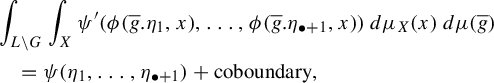
(1) We have that
for almost every $$ \begin{align*} &\int_{L \backslash G} \int_X \psi'(\phi(\overline{g}.\eta_1, x), \ldots, \phi(\overline{g}.\eta_{\bullet+1}, x))\, d\mu_X(x)\, d\mu(\overline{g})\\ &\quad = \psi(\eta_1, \ldots, \eta_{\bullet+1}) + \mathrm{coboundary}, \end{align*} $$
$(\eta _1,\ldots ,\eta _{\bullet+1}) \in (G/Q)^{\bullet+1}$
.
$$ \begin{align*} &\int_{L \backslash G} \int_X \psi'(\phi(\overline{g}.\eta_1, x), \ldots, \phi(\overline{g}.\eta_{\bullet+1}, x))\, d\mu_X(x)\, d\mu(\overline{g})\\ &\quad = \psi(\eta_1, \ldots, \eta_{\bullet+1}) + \mathrm{coboundary}, \end{align*} $$
$(\eta _1,\ldots ,\eta _{\bullet+1}) \in (G/Q)^{\bullet+1}$
.
-
(2) If
$\operatorname {\mathrm{H}}^{\bullet}_{cb}(G;\operatorname {\mathrm {\mathbb {R}}}) \cong \operatorname {\mathrm {\mathbb {R}}} \Psi (= \operatorname {\mathrm {\mathbb {R}}}[\psi ])$
, then there exists a real constant
$\lambda _{\psi ',\psi }(\sigma ) \in \operatorname {\mathrm {\mathbb {R}}}$
depending on
$\sigma ,\psi ',\psi $
such that for almost every
$$ \begin{align*} &\int_{L\backslash G} \int_X \psi'(\phi(\overline{g}.\eta_1, x), \ldots, \phi(\overline{g}.\eta_{\bullet+1}, x))\, d\mu_X(x)\,d\mu(\overline{g})\\ &\quad=\lambda_{\psi',\psi}(\sigma) \cdot \psi(\eta_1,\ldots,\eta_{\bullet+1}) +\mathrm{coboundary}, \end{align*} $$
$(\eta _1,\ldots ,\eta _{\bullet+1}) \in (G/Q)^{\bullet+1}$
.


Although this formula might appear slightly complicated at first sight, it contains all the ingredients for defining the multiplicative constant $\lambda _{\psi ',\psi }(\sigma )$
associated with a measurable cocycle
$\lambda _{\psi ',\psi }(\sigma )$
associated with a measurable cocycle $\sigma $
and two given bounded cochains
$\sigma $
and two given bounded cochains $\psi ,\psi '$
(Definition 3.21). When no coboundary terms appear in the previous formula, we provide an explicit upper bound for the multiplicative constant (Proposition 3.25). This leads to the definition of maximal measurable cocycles (Definition 3.26). Finally, under suitable hypothesis, we prove that a maximal cocycle is trivializable (Theorem 3.28), that is, it is cohomologous to a cocycle induced by a representation
$\psi ,\psi '$
(Definition 3.21). When no coboundary terms appear in the previous formula, we provide an explicit upper bound for the multiplicative constant (Proposition 3.25). This leads to the definition of maximal measurable cocycles (Definition 3.26). Finally, under suitable hypothesis, we prove that a maximal cocycle is trivializable (Theorem 3.28), that is, it is cohomologous to a cocycle induced by a representation $L \leq G \rightarrow G'$
.
$L \leq G \rightarrow G'$
.
This general framework has the great advantage that we can easily deduce several applications (§§3.5 and 7).
1.2 Cartan invariant of measurable cocycles
Let $\Gamma \leq \operatorname {\mathrm{PU}}(n,1)$
be a torsion-free lattice with
$\Gamma \leq \operatorname {\mathrm{PU}}(n,1)$
be a torsion-free lattice with $n \geq 2$
. The study of representations of
$n \geq 2$
. The study of representations of $\Gamma $
into
$\Gamma $
into $\operatorname {\mathrm{PU}}(m,1)$
dates back to the work of Goldman and Millson [Reference Goldman and MillsonGM87], Corlette [Reference CorletteCor88], and Toledo [Reference ToledoTol89]. In order to investigate rigidity properties of maximal representations
$\operatorname {\mathrm{PU}}(m,1)$
dates back to the work of Goldman and Millson [Reference Goldman and MillsonGM87], Corlette [Reference CorletteCor88], and Toledo [Reference ToledoTol89]. In order to investigate rigidity properties of maximal representations $\rho \colon \Gamma \rightarrow \operatorname {\mathrm{PU}}(m,1)$
, Burger and Iozzi [Reference Burger and IozziBI07b] defined the Cartan invariant
$\rho \colon \Gamma \rightarrow \operatorname {\mathrm{PU}}(m,1)$
, Burger and Iozzi [Reference Burger and IozziBI07b] defined the Cartan invariant $i_\rho $
associated with
$i_\rho $
associated with $\rho $
. Inspired by their work, we make use of our techniques to define the Cartan invariant
$\rho $
. Inspired by their work, we make use of our techniques to define the Cartan invariant $i(\sigma )$
for a measurable cocycle
$i(\sigma )$
for a measurable cocycle $\sigma :\Gamma \times X \rightarrow \operatorname {\mathrm{PU}}(m,1)$
, where
$\sigma :\Gamma \times X \rightarrow \operatorname {\mathrm{PU}}(m,1)$
, where $(X,\mu _X)$
is a standard Borel probability
$(X,\mu _X)$
is a standard Borel probability $\Gamma $
-space.
$\Gamma $
-space.
If the cocycle admits a boundary map (e.g. if it is non-elementary), the Cartan invariant can be realized as the multiplicative constant associated with $\sigma $
and the Cartan cocycles
$\sigma $
and the Cartan cocycles $c_n,c_m$
. More precisely, as an application of Proposition 1.1, we prove the following.
$c_n,c_m$
. More precisely, as an application of Proposition 1.1, we prove the following.
Proposition 1.2. Let $\Gamma \leq \operatorname {\mathrm{PU}}(n,1)$
be a torsion-free lattice and let
$\Gamma \leq \operatorname {\mathrm{PU}}(n,1)$
be a torsion-free lattice and let $(X,\mu _X)$
be a standard Borel probability space. Consider a non-elementary measurable cocycle
$(X,\mu _X)$
be a standard Borel probability space. Consider a non-elementary measurable cocycle $\sigma \colon \Gamma \times X \rightarrow \operatorname {\mathrm{PU}}(m,1)$
with boundary map
$\sigma \colon \Gamma \times X \rightarrow \operatorname {\mathrm{PU}}(m,1)$
with boundary map $\phi \colon \partial _\infty \operatorname {\mathrm {\mathbb {H}}}^n_{\operatorname {\mathrm {\mathbb {C}}}} \times X \rightarrow \partial _\infty \operatorname {\mathrm {\mathbb {H}}}^m_{\operatorname {\mathrm {\mathbb {C}}}}$
. Then, for every triple of pairwise distinct points
$\phi \colon \partial _\infty \operatorname {\mathrm {\mathbb {H}}}^n_{\operatorname {\mathrm {\mathbb {C}}}} \times X \rightarrow \partial _\infty \operatorname {\mathrm {\mathbb {H}}}^m_{\operatorname {\mathrm {\mathbb {C}}}}$
. Then, for every triple of pairwise distinct points $\xi _1,\xi _2,\xi _3 \in \partial _\infty \operatorname {\mathrm {\mathbb {H}}}^n_{\operatorname {\mathrm {\mathbb {C}}}}$
, we have
$\xi _1,\xi _2,\xi _3 \in \partial _\infty \operatorname {\mathrm {\mathbb {H}}}^n_{\operatorname {\mathrm {\mathbb {C}}}}$
, we have
 $$ \begin{align*} i(\sigma)c_n(\xi_1,\xi_2,\xi_3)=\int_{\Gamma \backslash \operatorname{\mathrm{PU}}(n,1)} \int_X c_m(\phi(\overline{g}\xi_1,x),\phi(\overline{g}\xi_2,x),\phi(\overline{g}\xi_3,x))\,d\mu(\overline{g})\,d\mu_X(x). \end{align*} $$
Here $\mu $
is a
$\mu $
is a $\operatorname {\mathrm{PU}}(n,1)$
-invariant probability measure on the quotient
$\operatorname {\mathrm{PU}}(n,1)$
-invariant probability measure on the quotient $\Gamma \backslash \operatorname {\mathrm{PU}}(n,1)$
.
$\Gamma \backslash \operatorname {\mathrm{PU}}(n,1)$
.
First we show that our Cartan invariant extends that defined for representations (Proposition 4.8). Moreover, using our results about the pullback along boundary maps, we prove that the Cartan invariant is constant along $\operatorname {\mathrm{PU}}(m,1)$
-cohomology classes and it has absolute value bounded by
$\operatorname {\mathrm{PU}}(m,1)$
-cohomology classes and it has absolute value bounded by $1$
(Proposition 4.9).
$1$
(Proposition 4.9).
Then, a natural problem is to provide a complete characterization of measurable cocycles whose Cartan invariant attains extremal values, that is, either $0$
or
$0$
or $1$
. Since we are not interested in elementary cocycles, we can assume the existence of a boundary map [Reference Monod and ShalomMS04, Proposition 3.3].
$1$
. Since we are not interested in elementary cocycles, we can assume the existence of a boundary map [Reference Monod and ShalomMS04, Proposition 3.3].
Following the work by Burger and Iozzi [Reference Burger and IozziBI12], we introduce the notion of totally real cocycles. A cocycle is totally real if it is cohomologous to a cocycle whose image is contained in a subgroup of $\operatorname {\mathrm{PU}}(m,1)$
preserving a totally geodesically embedded copy
$\operatorname {\mathrm{PU}}(m,1)$
preserving a totally geodesically embedded copy $\operatorname {\mathrm {\mathbb {H}}}^k_{\operatorname {\mathrm {\mathbb {R}}}} \subset \operatorname {\mathrm {\mathbb {H}}}^m_{\operatorname {\mathrm {\mathbb {R}}}}$
, for some
$\operatorname {\mathrm {\mathbb {H}}}^k_{\operatorname {\mathrm {\mathbb {R}}}} \subset \operatorname {\mathrm {\mathbb {H}}}^m_{\operatorname {\mathrm {\mathbb {R}}}}$
, for some $1 \leq k \leq m$
(Definition 5.1). Totally real cocycles can be easily constructed by taking the composition of a measure equivalence cocycle with a totally real representation.
$1 \leq k \leq m$
(Definition 5.1). Totally real cocycles can be easily constructed by taking the composition of a measure equivalence cocycle with a totally real representation.
We show that totally real cocycles have trivial Cartan invariant. The converse seems unlikely to hold in general. However, if X is $\Gamma $
-ergodic, we obtain the following.
$\Gamma $
-ergodic, we obtain the following.
Theorem 1.3. Let $\Gamma \leq \operatorname {\mathrm{PU}}(n,1)$
be a torsion-free lattice and let
$\Gamma \leq \operatorname {\mathrm{PU}}(n,1)$
be a torsion-free lattice and let $(X,\mu _X)$
be a standard Borel probability
$(X,\mu _X)$
be a standard Borel probability $\Gamma $
-space. Consider a non-elementary measurable cocycle
$\Gamma $
-space. Consider a non-elementary measurable cocycle $\sigma \colon \Gamma \times X \rightarrow \operatorname {\mathrm{PU}}(m,1)$
with boundary map
$\sigma \colon \Gamma \times X \rightarrow \operatorname {\mathrm{PU}}(m,1)$
with boundary map $\phi \colon \partial _\infty \mathbb {H}^n_{\operatorname {\mathrm {\mathbb {C}}}} \times X \rightarrow \partial _\infty \operatorname {\mathrm {\mathbb {H}}}^m_{\operatorname {\mathrm {\mathbb {C}}}}$
. Then the following hold:
$\phi \colon \partial _\infty \mathbb {H}^n_{\operatorname {\mathrm {\mathbb {C}}}} \times X \rightarrow \partial _\infty \operatorname {\mathrm {\mathbb {H}}}^m_{\operatorname {\mathrm {\mathbb {C}}}}$
. Then the following hold:
-
(1) if
$\sigma $
is totally real, then
$i(\sigma )=0$
; -
(2) if X is
$\Gamma $
-ergodic and
$\mathrm{H}^2(\phi )([c_m])=0$
, then
$\sigma $
is totally real.


The next step in our investigation is the study of the algebraic hull of a cocycle with non-vanishing pullback. Recall that the algebraic hull is the smallest algebraic group containing the image of a cocycle cohomologous to $\sigma $
(Definition 2.15).
$\sigma $
(Definition 2.15).
Theorem 1.4. Let $\Gamma \leq \mathrm{PU}(n,1)$
be a torsion-free lattice and let
$\Gamma \leq \mathrm{PU}(n,1)$
be a torsion-free lattice and let $(X,\mu _X)$
be an ergodic standard Borel probability
$(X,\mu _X)$
be an ergodic standard Borel probability $\Gamma $
-space. Consider a non-elementary measurable cocycle
$\Gamma $
-space. Consider a non-elementary measurable cocycle $\sigma \colon \Gamma \times X \rightarrow \operatorname {\mathrm{PU}}(m,1)$
with boundary map
$\sigma \colon \Gamma \times X \rightarrow \operatorname {\mathrm{PU}}(m,1)$
with boundary map $\phi \colon \partial _\infty \operatorname {\mathrm {\mathbb {H}}}^n_{\operatorname {\mathrm {\mathbb {C}}}} \times X \rightarrow \partial _\infty \operatorname {\mathrm {\mathbb {H}}}^m_{\operatorname {\mathrm {\mathbb {C}}}}$
. Let
$\phi \colon \partial _\infty \operatorname {\mathrm {\mathbb {H}}}^n_{\operatorname {\mathrm {\mathbb {C}}}} \times X \rightarrow \partial _\infty \operatorname {\mathrm {\mathbb {H}}}^m_{\operatorname {\mathrm {\mathbb {C}}}}$
. Let $\mathbf {L}$
be the algebraic hull of
$\mathbf {L}$
be the algebraic hull of $\sigma $
and denote by
$\sigma $
and denote by $L=\mathbf {L}(\operatorname {\mathrm {\mathbb {R}}})^\circ $
the connected component of the identity of the real points.
$L=\mathbf {L}(\operatorname {\mathrm {\mathbb {R}}})^\circ $
the connected component of the identity of the real points.
If $\operatorname {\mathrm{H}}^2(\Phi ^X)([c_m])\neq 0$
, then L is an almost direct product
$\operatorname {\mathrm{H}}^2(\Phi ^X)([c_m])\neq 0$
, then L is an almost direct product $K \cdot M$
, where K is compact and M is isomorphic to
$K \cdot M$
, where K is compact and M is isomorphic to $\mathrm{PU}(p,1)$
for some
$\mathrm{PU}(p,1)$
for some $1 \leq p \leq m$
.
$1 \leq p \leq m$
.
In particular, the symmetric space associated with L is a totally geodesically embedded copy of $\operatorname {\mathrm {\mathbb {H}}}^p_{\operatorname {\mathrm {\mathbb {C}}}}$
inside
$\operatorname {\mathrm {\mathbb {H}}}^p_{\operatorname {\mathrm {\mathbb {C}}}}$
inside $\operatorname {\mathrm {\mathbb {H}}}^m_{\operatorname {\mathrm {\mathbb {C}}}}$
.
$\operatorname {\mathrm {\mathbb {H}}}^m_{\operatorname {\mathrm {\mathbb {C}}}}$
.
We conclude with a complete characterization of maximal cocycles.
Theorem 1.5. Consider $n \geq 2$
. Let
$n \geq 2$
. Let $\Gamma \leq \operatorname {\mathrm{PU}}(n,1)$
be a torsion-free lattice. Let
$\Gamma \leq \operatorname {\mathrm{PU}}(n,1)$
be a torsion-free lattice. Let $(X,\mu _X)$
be an ergodic standard Borel probability
$(X,\mu _X)$
be an ergodic standard Borel probability $\Gamma $
-space. Consider a maximal measurable cocycle
$\Gamma $
-space. Consider a maximal measurable cocycle $\sigma \colon \Gamma \times X \rightarrow \operatorname {\mathrm{PU}}(m,1)$
. Let
$\sigma \colon \Gamma \times X \rightarrow \operatorname {\mathrm{PU}}(m,1)$
. Let $\mathbf {L}$
be the algebraic hull of
$\mathbf {L}$
be the algebraic hull of $\sigma $
and let
$\sigma $
and let $L=\mathbf {L}(\operatorname {\mathrm {\mathbb {R}}})^\circ $
be the connected component of the identity of the real points.
$L=\mathbf {L}(\operatorname {\mathrm {\mathbb {R}}})^\circ $
be the connected component of the identity of the real points.
Then, we have:
-
(1)
$m \geq n$
; -
(2) L is an almost direct product
$\mathrm{PU}(n,1) \cdot K$
, where K is compact; -
(3)
$\sigma $
is cohomologous to the cocycle
$\sigma _i$
associated with the standard lattice embedding
$i \colon \Gamma \to \operatorname {\mathrm{PU}}(m,1)$
(possibly modulo the compact subgroup K when
$m>n$
).


Since one of the authors together with Sarti recently proved a generalization of the previous theorem for cocycles with target $\mathrm{PU}(p,q)$
[Reference Sarti and SaviniSS21, Theorem 2], we will mainly refer to their more complete result for the proof.
$\mathrm{PU}(p,q)$
[Reference Sarti and SaviniSS21, Theorem 2], we will mainly refer to their more complete result for the proof.
1.3 Plan of the paper
In §2, we recall some preliminary definitions and results that we need in the paper. We report the definitions of amenable action, measurable cocycle, boundary map, and algebraic hull in §2.1. We then review Burger and Monod’s functorial approach to continuous bounded cohomology (§2.2) and we conclude this preliminary section with the definition of transfer maps (§2.3).
Section 3 is devoted to the description of the general framework in which we study multiplicative constants associated with measurable cocycles. There, we first define the pullback along a measurable cocycle and along its boundary map (§3.1). Then, we compare our definition with the usual one given for representations (§3.2). In §3.3, we state our multiplicative formula (Proposition 1.1) and we introduce the notion of a multiplicative constant associated with a measurable cocycle. We conclude the section studying the notion of maximality (§3.4) and showing some applications of the previous results (§3.5).
Section 4 contains the new application of our machinery. There, we introduce and study the Cartan invariant of measurable cocycles (§4). We prove that it is a multiplicative constant (Proposition 1.2) and it extends the same invariant for representations (Proposition 4.8). Moreover, we show that the Cartan invariant has a bounded absolute value in Proposition 4.9.
In §5, we define totally real cocycles and we prove Theorem 5.4. Then in §6, we study maximal measurable cocycles and we prove both Theorem 6.1 and Theorem 6.2. We conclude with some remarks about recent applications of our theory in §7.
2 Preliminary definitions and results
2.1 Amenability and measurable cocycles
In this section, we are going to recall some classic definitions related to both amenability and measurable cocycles. We start by fixing the following notation.
-
• Let G be a locally compact second countable group endowed with its Haar measurable structure.
-
• Let
$(X,\mu )$
be a standard Borel measure G-space, that is a standard Borel measure space endowed with a measure-preserving G-action.

If $\mu $
is a probability measure, we will refer to
$\mu $
is a probability measure, we will refer to $(X, \mu )$
as a standard Borel probability G-space. Given another measure space
$(X, \mu )$
as a standard Borel probability G-space. Given another measure space $(Y,\nu )$
, we denote by
$(Y,\nu )$
, we denote by $\mathrm{Meas}(X,Y)$
the space of measurable functions from X to Y endowed with the topology of convergence in measure.
$\mathrm{Meas}(X,Y)$
the space of measurable functions from X to Y endowed with the topology of convergence in measure.
Remark 2.1. In the literature about the ergodic version of simplicial volume [Reference Campagnolo and CorroCC21, Reference Fauser, Friedl and LöhFFL19, Reference Francaviglia, Frigerio and MartelliFFM12, Reference Fauser, Löh, Moraschini and QuintanilhaFLMQ21, Reference Frigerio, Löh, Pagliantini and SauerFLPS16, Reference Löh and PagliantiniLP16, Reference SauerSau02, Reference SchmidtSch05], it is often convenient to work with essentially free actions. For this reason, one might find it reasonable to stick with the same assumptions also here working with the dual notion of bounded cohomology. However, it is easy to check that every probability measure-preserving action can be promoted to an essentially free action just by taking the product with an essentially free action and considering the diagonal action on that product.
We recall now some definitions about amenability. We mainly refer the reader to the books by Zimmer [Reference ZimmerZim84, §4.3] and by Monod [Reference MonodMon01, §5.3] for further details about this topic.
Let $\operatorname {\mathrm{L}}^\infty (G;\operatorname {\mathrm {\mathbb {R}}})$
denote the space of essentially bounded real functions over G. Then, G acts on
$\operatorname {\mathrm{L}}^\infty (G;\operatorname {\mathrm {\mathbb {R}}})$
denote the space of essentially bounded real functions over G. Then, G acts on $\operatorname {\mathrm{L}}^\infty (G;\operatorname {\mathrm {\mathbb {R}}})$
as follows:
$\operatorname {\mathrm{L}}^\infty (G;\operatorname {\mathrm {\mathbb {R}}})$
as follows:
 $$ \begin{align*}g.f (g_0) = f(g^{-1} g_0), \end{align*} $$
for all $g, g_0 \in \, G$
and
$g, g_0 \in \, G$
and $f \in \, \operatorname {\mathrm{L}}^\infty (G;\operatorname {\mathrm {\mathbb {R}}})$
.
$f \in \, \operatorname {\mathrm{L}}^\infty (G;\operatorname {\mathrm {\mathbb {R}}})$
.
Definition 2.2. A mean on $\operatorname {\mathrm{L}}^\infty (G;\operatorname {\mathrm {\mathbb {R}}})$
is a continuous linear functional
$\operatorname {\mathrm{L}}^\infty (G;\operatorname {\mathrm {\mathbb {R}}})$
is a continuous linear functional
 $$ \begin{align*}m \colon \operatorname{\mathrm{L}}^\infty(G;\operatorname{\mathrm{\mathbb{R}}}) \rightarrow \operatorname{\mathrm{\mathbb{R}}}, \end{align*} $$
such that $m(f)\geq 0$
whenever
$m(f)\geq 0$
whenever $f \geq 0$
and
$f \geq 0$
and $m(\chi _G)=1$
, where
$m(\chi _G)=1$
, where $\chi _G$
denotes the characteristic function on G.
$\chi _G$
denotes the characteristic function on G.
We say that a mean is left invariant if for all $g \in \, G$
and
$g \in \, G$
and $f \in \, \operatorname {\mathrm{L}}^\infty (G;\operatorname {\mathrm {\mathbb {R}}})$
we have
$f \in \, \operatorname {\mathrm{L}}^\infty (G;\operatorname {\mathrm {\mathbb {R}}})$
we have $m(g.f) = m(f)$
.
$m(g.f) = m(f)$
.
A group is amenable if it admits a left-invariant mean.
Example 2.3. The following families are examples of amenable groups:
-
(1) abelian groups [Reference ZimmerZim84, Theorem 4.1.2];
-
(2) finite/compact groups [Reference ZimmerZim84, Theorem 4.1.5];
-
(3) extensions of amenable groups by amenable groups [Reference ZimmerZim84, Proposition 4.1.6];
-
(4) let G be a Lie group and let
$P \subset G$
be any minimal parabolic subgroup. Then, P is an extension of a solvable group by a compact group, from which it is amenable [Reference ZimmerZim84, Corollary 4.1.7].

In what follows, we will need a more general notion of amenability which is related to group actions. In fact, amenable spaces and amenable actions will play a crucial role in the functorial approach to the computation of continuous bounded cohomology (§2.2). Following Monod’s convention, we begin by defining regular G-spaces [Reference MonodMon01, Definition 2.1.1].
Definition 2.4. Let G be a locally compact second countable group and let S be a standard Borel space with a measurable G-action which preserve a measure class. We say that $(S, \mu )$
is a regular G-space if the previous measure class contains a probability measure
$(S, \mu )$
is a regular G-space if the previous measure class contains a probability measure $\mu $
such that the isometric action
$\mu $
such that the isometric action $R \colon G \curvearrowright \operatorname {\mathrm{L}}^1(S, \mu )$
defined by
$R \colon G \curvearrowright \operatorname {\mathrm{L}}^1(S, \mu )$
defined by
 $$ \begin{align*}(R(g).f)(s) = f(g^{-1}.s) \frac{d g^{-1}\mu}{d\mu}(s) \end{align*} $$
is continuous. Here, $d g^{-1}\mu /d\mu $
denotes the Radon–Nikodým derivative.
$d g^{-1}\mu /d\mu $
denotes the Radon–Nikodým derivative.
Example 2.5. Let G be a locally compact second countable group, then the following are examples of regular G-spaces [Reference MonodMon01, Example 2.1.2].
-
(1) If G is endowed with its Haar measure, then G is a regular G-space.
-
(2) If Q is a closed subgroup of G, then
$G/Q$
endowed with the natural almost invariant measure is a regular G-space. -
(3) Furstenberg–Poisson boundaries [Reference FurstenbergFur73, Reference FurstenbergFur81] associated with a probability measure on G are regular G-spaces.

The notion of regular G-spaces allows us to introduce the definitions of amenable actions and amenable spaces [Reference MonodMon01, Theorem 5.3.2].
Definition 2.6. Let G be a locally compact second countable group and let $(S,\mu )$
be a regular G-space. We say that the action of G on
$(S,\mu )$
be a regular G-space. We say that the action of G on $(S,\mu )$
is amenable if there exists a continuous norm-one G-equivariant linear operator
$(S,\mu )$
is amenable if there exists a continuous norm-one G-equivariant linear operator
 $$ \begin{align*}p \colon\! \operatorname{\mathrm{L}}^\infty(G \times S;\operatorname{\mathrm{\mathbb{R}}}) \rightarrow \operatorname{\mathrm{L}}^\infty(S;\operatorname{\mathrm{\mathbb{R}}}), \end{align*} $$
with the following two properties: first, $p(\chi _{G \times S})=\chi _S$
; second, for all
$p(\chi _{G \times S})=\chi _S$
; second, for all $f \in \, \operatorname {\mathrm{L}}^\infty (G \times S)$
and for all measurable sets
$f \in \, \operatorname {\mathrm{L}}^\infty (G \times S)$
and for all measurable sets $A \subset S$
, we have
$A \subset S$
, we have $p(f \cdot \chi _{G \times A}) = p(f) \cdot \chi _A$
.
$p(f \cdot \chi _{G \times A}) = p(f) \cdot \chi _A$
.
If the action by G on $(S, \mu )$
is amenable, then we say that
$(S, \mu )$
is amenable, then we say that $(S,\mu )$
is an amenable G-space.
$(S,\mu )$
is an amenable G-space.
Remark 2.7. The previous definition extends the notion of amenable groups in the following sense: a group is amenable if and only if every regular G-space is an amenable G-space [Reference MonodMon01, Theorem 5.3.9].
Amenable actions not only characterize groups but also subgroups. By Example 2.5.2, given a closed subgroup $Q \subset G$
, the quotient
$Q \subset G$
, the quotient $G/ Q$
is a regular G-space. Additionally, we have that Q is amenable if and only if the G-action on
$G/ Q$
is a regular G-space. Additionally, we have that Q is amenable if and only if the G-action on $G/Q$
is amenable [Reference ZimmerZim84, Proposition 4.3.2]. Hence, Example 2.3.4 shows that if G is a Lie group and
$G/Q$
is amenable [Reference ZimmerZim84, Proposition 4.3.2]. Hence, Example 2.3.4 shows that if G is a Lie group and $P \subset G$
is any minimal parabolic subgroup, then the G-action on the quotient
$P \subset G$
is any minimal parabolic subgroup, then the G-action on the quotient $G \curvearrowright G/P$
is amenable. This applies to the Furstenberg–Poisson boundary of a Lie group (being identified with
$G \curvearrowright G/P$
is amenable. This applies to the Furstenberg–Poisson boundary of a Lie group (being identified with $G/P$
).
$G/P$
).
We recall now the notion of measurable cocycles and some of their properties.
Definition 2.8. Let G and H be locally compact groups and let $(X,\mu )$
be a standard Borel probability G-space. A measurable cocycle (or, simply cocycle) is a measurable map
$(X,\mu )$
be a standard Borel probability G-space. A measurable cocycle (or, simply cocycle) is a measurable map $\sigma \colon G \times X \rightarrow H$
satisfying the following formula:
$\sigma \colon G \times X \rightarrow H$
satisfying the following formula:
 $$ \begin{align} \sigma(g_1g_2,x)=\sigma(g_1,g_2.x)\sigma(g_2,x), \end{align} $$
for almost every $g_1,g_2 \in G$
and almost every
$g_1,g_2 \in G$
and almost every $x \in X$
. Here,
$x \in X$
. Here, $g_2.x$
denotes the action by
$g_2.x$
denotes the action by $g_2 \in G$
on
$g_2 \in G$
on $x \in \, X$
.
$x \in \, X$
.
Associated with measurable cocycles, there exists the crucial notion of a boundary map.
Definition 2.9. Let G and H be two locally compact groups and let $Q \leq G$
be a closed amenable subgroup. Let
$Q \leq G$
be a closed amenable subgroup. Let $(X,\mu )$
be a standard Borel probability G-space and let
$(X,\mu )$
be a standard Borel probability G-space and let $(Y,\nu )$
be a measure space on which H acts by preserving the measure class of
$(Y,\nu )$
be a measure space on which H acts by preserving the measure class of $\nu $
. Given a measurable cocycle
$\nu $
. Given a measurable cocycle $\sigma \colon G \times X \rightarrow H$
, we say that a measurable map
$\sigma \colon G \times X \rightarrow H$
, we say that a measurable map $\phi \colon G/Q \times X \rightarrow Y$
is
$\phi \colon G/Q \times X \rightarrow Y$
is $\sigma $
-equivariant if we have
$\sigma $
-equivariant if we have
 $$ \begin{align*}\phi(g.\eta,g.x)=\sigma(g,x)\phi(\eta,x), \end{align*} $$
for almost every $g \in G,\eta \in G/Q$
and
$g \in G,\eta \in G/Q$
and $x \in X$
.
$x \in X$
.
A (generalized) boundary map associated with $\sigma $
is a
$\sigma $
is a $\sigma $
-equivariant measurable map.
$\sigma $
-equivariant measurable map.
We will make use of generalized boundary maps in §3.1, where we will explain how to compute the pullback in continuous bounded cohomology.
Remark 2.10. It is quite natural to ask when a (generalized) boundary map actually exists. Let $G(n)=\mathrm{Isom}(\operatorname {\mathrm {\mathbb {H}}}^n_{K})$
be the isometry group of the K-hyperbolic space, where K is either
$G(n)=\mathrm{Isom}(\operatorname {\mathrm {\mathbb {H}}}^n_{K})$
be the isometry group of the K-hyperbolic space, where K is either $\operatorname {\mathrm {\mathbb {R}}}$
or
$\operatorname {\mathrm {\mathbb {R}}}$
or $\operatorname {\mathrm {\mathbb {C}}}$
. Given a lattice
$\operatorname {\mathrm {\mathbb {C}}}$
. Given a lattice $\Gamma \leq G(n)$
, let us consider a standard Borel probability
$\Gamma \leq G(n)$
, let us consider a standard Borel probability $\Gamma $
-space
$\Gamma $
-space $(X,\mu _X)$
and a measurable cocycle
$(X,\mu _X)$
and a measurable cocycle $\sigma :\Gamma \times X \rightarrow G(m)$
. In the previous situation, Monod and Shalom [Reference Monod and ShalomMS04, Proposition 3.3] proved that if the cocycle
$\sigma :\Gamma \times X \rightarrow G(m)$
. In the previous situation, Monod and Shalom [Reference Monod and ShalomMS04, Proposition 3.3] proved that if the cocycle $\sigma $
is non-elementary, then there exists an essentially unique boundary map,
$\sigma $
is non-elementary, then there exists an essentially unique boundary map,
 $$ \begin{align*}\phi:\partial_\infty \operatorname{\mathrm{\mathbb{H}}}^n_{K} \times X \rightarrow \partial_\infty \operatorname{\mathrm{\mathbb{H}}}^m_{K}. \end{align*} $$
The notion of non-elementary cocycle relies on the definition of an algebraic hull (Definition 2.15) and this will be explained more carefully later in this paper.
Additionally, in the case of higher rank lattices, there are some relevant results about the existence of boundary maps. Indeed a key step in the proof of Zimmer’s super-rigidity theorem [Reference ZimmerZim80, Theorem 4.1] is to prove the existence of generalized boundary maps for Zariski dense measurable cocycles (see Definition 2.15).
Since equation (1) suggests that $\sigma $
can be interpreted as a Borel
$\sigma $
can be interpreted as a Borel $1$
-cocycle in
$1$
-cocycle in $\mathrm{Meas}(G,\mathrm{Meas}(X,H))$
[Reference Feldman and MooreFM77], it is natural to introduce the definition of cohomologous cocycles.
$\mathrm{Meas}(G,\mathrm{Meas}(X,H))$
[Reference Feldman and MooreFM77], it is natural to introduce the definition of cohomologous cocycles.
Definition 2.11. Let $\sigma \colon G \times X \rightarrow H$
be a measurable cocycle between locally compact groups. Let
$\sigma \colon G \times X \rightarrow H$
be a measurable cocycle between locally compact groups. Let $f \colon X \rightarrow H$
be a measurable map. We define the twisted cocycle associated with
$f \colon X \rightarrow H$
be a measurable map. We define the twisted cocycle associated with $\sigma $
and f as
$\sigma $
and f as
 $$ \begin{align*}f.\sigma \colon G \times X \rightarrow H, \quad (f.\sigma)(g,x) := f(g.x)^{-1}\sigma(g,x)f(x), \end{align*} $$
for almost every $g \in G$
and almost every
$g \in G$
and almost every $x \in X$
.
$x \in X$
.
We say that two measurable cocycles $\sigma _1,\sigma _2\colon G \times X \rightarrow H$
are cohomologous if there exists a measurable function
$\sigma _1,\sigma _2\colon G \times X \rightarrow H$
are cohomologous if there exists a measurable function $f \colon X \rightarrow H$
such that
$f \colon X \rightarrow H$
such that
 $$ \begin{align*}\sigma_2=f.\sigma_1. \end{align*} $$
Similarly, we say that $\sigma _1$
and
$\sigma _1$
and $\sigma _2$
are cohomologous modulo a closed subgroup
$\sigma _2$
are cohomologous modulo a closed subgroup $C \leq H$
if
$C \leq H$
if
 $$ \begin{align*}\sigma_2=f.\sigma_1\! \mod C, \end{align*} $$
that is
 $$ \begin{align*}\sigma_2(g,x) \cdot (f.\sigma_1(g,x))^{-1} \in C, \end{align*} $$
for almost every $g \in G, x \in X$
.
$g \in G, x \in X$
.
When a measurable cocycle $\sigma $
admits a generalized boundary map, then all its cohomologous cocycles share the same property.
$\sigma $
admits a generalized boundary map, then all its cohomologous cocycles share the same property.
Definition 2.12. Let $\sigma \colon G \times X \rightarrow H$
be a measurable cocycle with generalized boundary map
$\sigma \colon G \times X \rightarrow H$
be a measurable cocycle with generalized boundary map $\phi \colon G/Q \times X \rightarrow Y$
. Given a measurable function
$\phi \colon G/Q \times X \rightarrow Y$
. Given a measurable function $f \colon X \rightarrow H$
, the twisted boundary map associated with f and
$f \colon X \rightarrow H$
, the twisted boundary map associated with f and $\phi $
is defined as
$\phi $
is defined as
 $$ \begin{align*}f.\phi \colon G/Q \times X \rightarrow Y, \quad (f.\phi)(\eta,x) := f(x)^{-1}\phi(\eta,x), \end{align*} $$
for almost every $g \in G,\eta \in G/Q$
and
$g \in G,\eta \in G/Q$
and $x \in X$
.
$x \in X$
.
Remark 2.13. Let $\sigma , \sigma ' \colon G \times X \rightarrow H$
be two cohomologous cocycles and let
$\sigma , \sigma ' \colon G \times X \rightarrow H$
be two cohomologous cocycles and let $f \colon X \rightarrow H$
be the measurable map such that
$f \colon X \rightarrow H$
be the measurable map such that $\sigma ' = f.\sigma $
. If
$\sigma ' = f.\sigma $
. If $\sigma $
admits a generalized boundary map
$\sigma $
admits a generalized boundary map $\phi $
, then the twisted boundary map associated with f and
$\phi $
, then the twisted boundary map associated with f and $\phi $
is a generalized boundary map associated with
$\phi $
is a generalized boundary map associated with $\sigma '$
.
$\sigma '$
.
Representations provide special cases of measurable cocycles.
Definition 2.14. Let $\rho \colon G \rightarrow H$
be a continuous representation and let
$\rho \colon G \rightarrow H$
be a continuous representation and let $(X,\mu )$
be a standard Borel probability G-space. The cocycle associated with the representation
$(X,\mu )$
be a standard Borel probability G-space. The cocycle associated with the representation $\rho $
is defined as
$\rho $
is defined as
 $$ \begin{align*}\sigma_\rho \colon G \times X \rightarrow H, \quad \sigma_\rho(g,x)=\rho(g), \end{align*} $$
for every $g \in G$
and almost every
$g \in G$
and almost every $x \in X$
.
$x \in X$
.
Given a representation $\rho \colon G \rightarrow H$
, one can obtain useful information about
$\rho \colon G \rightarrow H$
, one can obtain useful information about $\rho $
by studying the closure of the image
$\rho $
by studying the closure of the image $\overline {\rho (\Gamma )}$
as a subgroup of H. On the other hand, in general, the image of a measurable cocycle does not have any nice algebraic structure. Nevertheless, when H is assumed to be an algebraic group, we can give the following.
$\overline {\rho (\Gamma )}$
as a subgroup of H. On the other hand, in general, the image of a measurable cocycle does not have any nice algebraic structure. Nevertheless, when H is assumed to be an algebraic group, we can give the following.
Definition 2.15. Let $\mathbf {H}$
be a real algebraic group and denote by
$\mathbf {H}$
be a real algebraic group and denote by $H=\mathbf {H}(\operatorname {\mathrm {\mathbb {R}}})$
the set of real points of
$H=\mathbf {H}(\operatorname {\mathrm {\mathbb {R}}})$
the set of real points of $\mathbf {H}$
. The algebraic hull of a measurable cocycle
$\mathbf {H}$
. The algebraic hull of a measurable cocycle $\sigma \colon G \times X \rightarrow H$
is the (conjugacy class of the) smallest algebraic subgroup
$\sigma \colon G \times X \rightarrow H$
is the (conjugacy class of the) smallest algebraic subgroup $\mathbf {L} \leq \mathbf {H}$
such that
$\mathbf {L} \leq \mathbf {H}$
such that $\mathbf {L}(\operatorname {\mathrm {\mathbb {R}}})^\circ $
contains the image of a cocycle cohomologous to
$\mathbf {L}(\operatorname {\mathrm {\mathbb {R}}})^\circ $
contains the image of a cocycle cohomologous to $\sigma $
. Here,
$\sigma $
. Here, $\mathbf {L}(\operatorname {\mathrm {\mathbb {R}}})^\circ $
denotes the connected component of the neutral element.
$\mathbf {L}(\operatorname {\mathrm {\mathbb {R}}})^\circ $
denotes the connected component of the neutral element.
Remark 2.16. The algebraic hull is well defined by the Noetherian property of algebraic groups. Moreover, it only depends on the cohomology class of the cocycle $\sigma $
[Reference ZimmerZim84, Proposition 9.2.1].
$\sigma $
[Reference ZimmerZim84, Proposition 9.2.1].
We will use the previous definition when we will work with totally real cocycles (§5) and when we will investigate the properties of cocycles with non-vanishing pullback (Theorem 6.1).
2.2 Bounded cohomology and its functorial approach
In this section, we are going to recall the definitions and the properties of both continuous and continuous bounded cohomology that we will need in what follows.
We first introduce continuous (bounded) cohomology via the homogeneous resolution and then, following the work by Burger and Monod [Reference Burger and MonodBM02, Reference MonodMon01], we describe it in terms of strong resolutions by relatively injective modules.
Definition 2.17. Let G be a locally compact group. A Banach G-module $(E, \pi )$
is a Banach space E endowed with a G-action induced by a representation
$(E, \pi )$
is a Banach space E endowed with a G-action induced by a representation $\pi \colon G \to \mathrm{Isom}(E)$
, or equivalently a G-action via linear isometries:
$\pi \colon G \to \mathrm{Isom}(E)$
, or equivalently a G-action via linear isometries:
 $$ \begin{align*} \theta_\pi \colon G \times E &\to E, \\ \theta_\pi (g, v) &:= \pi (g) v. \end{align*} $$
We say that a Banach G-module $(E, \pi )$
is continuous if the map
$(E, \pi )$
is continuous if the map $\theta (\cdot , v)$
is continuous for all
$\theta (\cdot , v)$
is continuous for all $v \in \, E$
. Finally, we denote by
$v \in \, E$
. Finally, we denote by $E^G$
the submodule of G-invariant vectors in E, that is, the space of vectors v such that
$E^G$
the submodule of G-invariant vectors in E, that is, the space of vectors v such that $\theta (g, v) = v$
for all
$\theta (g, v) = v$
for all $g \in \, G$
.
$g \in \, G$
.
Notation 2.18. In the following, $\mathbb {R}$
will denote the Banach G-module of trivial real coefficients. In other words, it is endowed with the trivial G-action:
$\mathbb {R}$
will denote the Banach G-module of trivial real coefficients. In other words, it is endowed with the trivial G-action: $\pi (g) v = v$
for all
$\pi (g) v = v$
for all $v \in \, \mathbb {R}$
and
$v \in \, \mathbb {R}$
and $g \in \, G$
.
$g \in \, G$
.
Example 2.19. Let $(E, \pi )$
be a Banach G-module. Then, the space of continuous E-valued functions
$(E, \pi )$
be a Banach G-module. Then, the space of continuous E-valued functions
 $$ \begin{align*}\mathrm{C}_{c}^{\bullet}(G; E) := \{f \colon G^{\bullet+1} \rightarrow E \, | \, f\ \mbox{is continuous} \} \end{align*} $$
is a continuous Banach G-module with the following action:
 $$ \begin{align} g.f (h_1, \ldots, h_{\bullet +1}) = \pi(g) f(g^{-1} h_1, \ldots, g^{-1} h_{\bullet+1}), \end{align} $$
for all $g, h_1, \ldots , h_{\bullet+1} \in \, G$
.
$g, h_1, \ldots , h_{\bullet+1} \in \, G$
.
The spaces of continuous E-valued functions give rise to a cochain complex $(\mathrm{C}_{c}^{\bullet}(G; E), \delta ^{\bullet})$
together with the standard homogeneous coboundary operator
$(\mathrm{C}_{c}^{\bullet}(G; E), \delta ^{\bullet})$
together with the standard homogeneous coboundary operator
 $$ \begin{align*}\delta^{\bullet} \colon \mathrm{C}_{c}^{\bullet}(G; E) \rightarrow \mathrm{C}_{c}^{\bullet + 1}(G; E), \end{align*} $$
 $$ \begin{align*}\delta^{\bullet} (f) (g_1, \ldots, g_{\bullet + 2}) := \sum_{j = 1}^{\bullet + 2} (-1)^{j - 1} f(g_1, \ldots, g_{j-1}, g_{j+1} \ldots, g_{\bullet + 2}). \end{align*} $$
Since this complex is exact, we are going to focus our attention on the subcomplex of G-invariant vectors $(\operatorname {\mathrm{C}}_c^{\bullet}(G; E)^G, \delta ^{\bullet})$
.
$(\operatorname {\mathrm{C}}_c^{\bullet}(G; E)^G, \delta ^{\bullet})$
.
Definition 2.20. The continuous cohomology of G with coefficients in E, denoted by $\operatorname {\mathrm{H}}_{c}^{\bullet}(G; E)$
, is the cohomology of the complex
$\operatorname {\mathrm{H}}_{c}^{\bullet}(G; E)$
, is the cohomology of the complex $(\operatorname {\mathrm{C}}_{c}^{\bullet}(G; E)^G, \delta ^{\bullet})$
.
$(\operatorname {\mathrm{C}}_{c}^{\bullet}(G; E)^G, \delta ^{\bullet})$
.
Remark 2.21. If G is a discrete group, then there is no difference between continuous and ordinary cohomology. Hence, in this situation, we will usually drop the subscript c from the notation.
Since $(E, \lVert \cdot \rVert _E)$
is a Banach space, the Banach G-module
$(E, \lVert \cdot \rVert _E)$
is a Banach space, the Banach G-module $\operatorname {\mathrm{C}}_c^{\bullet}(G; E)$
has a natural
$\operatorname {\mathrm{C}}_c^{\bullet}(G; E)$
has a natural $\operatorname {\mathrm{L}}^\infty $
-norm: For every
$\operatorname {\mathrm{L}}^\infty $
-norm: For every $f \in \, \operatorname {\mathrm{C}}_c^{\bullet}(G; E)$
, we have
$f \in \, \operatorname {\mathrm{C}}_c^{\bullet}(G; E)$
, we have
 $$ \begin{align*}\lVert f \rVert_\infty := \sup \{ \lVert f(g_1, \ldots, g_{\bullet + 1} )\rVert_E \, | \, g_1, \ldots, g_{\bullet +1} \in \, G \}. \end{align*} $$
A continuous function is said to be bounded if its $\operatorname {\mathrm{L}}^\infty $
-norm is finite. Let
$\operatorname {\mathrm{L}}^\infty $
-norm is finite. Let $\operatorname {\mathrm{C}}_{cb}^{\bullet}(G; E) \subset \operatorname {\mathrm{C}}_c^{\bullet}(G; E)$
be the subspace of continuous bounded functions. By linearity, the coboundary operator
$\operatorname {\mathrm{C}}_{cb}^{\bullet}(G; E) \subset \operatorname {\mathrm{C}}_c^{\bullet}(G; E)$
be the subspace of continuous bounded functions. By linearity, the coboundary operator $\delta ^{\bullet}$
preserves boundedness, so we can restrict
$\delta ^{\bullet}$
preserves boundedness, so we can restrict $\delta ^{\bullet}$
to the space of continuous bounded G-invariant functions
$\delta ^{\bullet}$
to the space of continuous bounded G-invariant functions $\operatorname {\mathrm{C}}_{cb}^{\bullet}(G;E)^G$
. Then we get the following complex:
$\operatorname {\mathrm{C}}_{cb}^{\bullet}(G;E)^G$
. Then we get the following complex:
 $$ \begin{align*}(\operatorname{\mathrm{C}}_{cb}^{\bullet}(G; E)^G, \delta^{\bullet}). \end{align*} $$
Definition 2.22. The continuous bounded cohomology of G with coefficients in E, denoted by $\operatorname {\mathrm{H}}_{cb}^{\bullet}(G; E)$
, is the cohomology of the complex
$\operatorname {\mathrm{H}}_{cb}^{\bullet}(G; E)$
, is the cohomology of the complex $(\operatorname {\mathrm{C}}_{cb}^{\bullet}(G; E)^G, \delta ^{\bullet})$
.
$(\operatorname {\mathrm{C}}_{cb}^{\bullet}(G; E)^G, \delta ^{\bullet})$
.
Remark 2.23. If $L \subset G$
is a closed subgroup, then we can compute the continuous bounded cohomology of L with E-coefficients as the cohomology of the complex
$L \subset G$
is a closed subgroup, then we can compute the continuous bounded cohomology of L with E-coefficients as the cohomology of the complex $(\operatorname {\mathrm{C}}_{cb}^{\bullet}(G;E)^L, \delta ^{\bullet})$
. Here, the L-action is the restriction of the natural G-action on
$(\operatorname {\mathrm{C}}_{cb}^{\bullet}(G;E)^L, \delta ^{\bullet})$
. Here, the L-action is the restriction of the natural G-action on $\operatorname {\mathrm{C}}_{cb}^{\bullet}(G;E)$
[Reference MonodMon01, Corollary 7.4.10].
$\operatorname {\mathrm{C}}_{cb}^{\bullet}(G;E)$
[Reference MonodMon01, Corollary 7.4.10].
The $\operatorname {\mathrm{L}}^\infty $
-norm defined on cochains induces a canonical
$\operatorname {\mathrm{L}}^\infty $
-norm defined on cochains induces a canonical $\operatorname {\mathrm{L}}^\infty $
-seminorm in cohomology given by
$\operatorname {\mathrm{L}}^\infty $
-seminorm in cohomology given by
 $$ \begin{align*}\lVert f \rVert_\infty := \inf \{ \lVert \psi \rVert_\infty \ | \ [\psi]=f \}. \end{align*} $$
We say that an isomorphism between seminormed cohomology groups is isometric if the corresponding seminorms are preserved.
Beyond the difference determined by the quotient seminorm, one can study the gap between continuous cohomology and continuous bounded cohomology via the map induced in cohomology by the inclusion $ i \colon \! \operatorname {\mathrm{C}}_{cb}^{\bullet}(G; E)^G \rightarrow \operatorname {\mathrm{C}}^{\bullet}_{c}(G; E)^G$
. The resulting map
$ i \colon \! \operatorname {\mathrm{C}}_{cb}^{\bullet}(G; E)^G \rightarrow \operatorname {\mathrm{C}}^{\bullet}_{c}(G; E)^G$
. The resulting map
 $$ \begin{align*}\operatorname{\mathrm{comp}}_G^{\bullet} \colon\! \operatorname{\mathrm{H}}_{cb}^{\bullet}(G; E) \rightarrow \operatorname{\mathrm{H}}_c^{\bullet}(G; E)\end{align*} $$
is called a comparison map.
In the following, we will need an alternative description of continuous bounded cohomology in terms of strong resolutions via relatively injective modules. Since we will not make an explicit use of these notions, we refer the reader to Monod’s book for a broad discussion on them [Reference MonodMon01, §§4.1 and 7.1]. The main result in this direction is the following.
Theorem 2.24. [Reference MonodMon01, Theorem 7.2.1]
Let G be a locally compact group and let $(E, \pi )$
be a Banach G-module. Then, for every strong resolution
$(E, \pi )$
be a Banach G-module. Then, for every strong resolution $(E^{\bullet}, \delta ^{\bullet})$
of E via relatively injective G-modules, the cohomology of the complex of G-invariants
$(E^{\bullet}, \delta ^{\bullet})$
of E via relatively injective G-modules, the cohomology of the complex of G-invariants $\operatorname {\mathrm{H}}^n((E^{\bullet})^G, \delta ^{\bullet}))$
is isomorphic as a topological vector space to the continuous bounded cohomology
$\operatorname {\mathrm{H}}^n((E^{\bullet})^G, \delta ^{\bullet}))$
is isomorphic as a topological vector space to the continuous bounded cohomology $\operatorname {\mathrm{H}}^n_{cb}(G; E)$
, for every
$\operatorname {\mathrm{H}}^n_{cb}(G; E)$
, for every $n \geq 0$
.
$n \geq 0$
.
We now describe a strong resolution via relatively injective modules which allows us to compute bounded cohomology isometrically. Let G be a locally compact second countable group. Let $(E, \pi , \lVert \cdot \rVert _E)$
be a Banach G-module such that E is the dual of some Banach space. This implies that E can be endowed with the weak-
$(E, \pi , \lVert \cdot \rVert _E)$
be a Banach G-module such that E is the dual of some Banach space. This implies that E can be endowed with the weak- $^*$
topology and the associated weak-
$^*$
topology and the associated weak- $^*$
Borel structure. Moreover, let
$^*$
Borel structure. Moreover, let $(S, \mu )$
be a regular G-space. We have the following.
$(S, \mu )$
be a regular G-space. We have the following.
Definition 2.25. We define the Banach G-module of bounded weak- $^*$
measurable E-valued functions on S to be the Banach space
$^*$
measurable E-valued functions on S to be the Banach space
 $$ \begin{align*}&\mathcal{B}^{\infty}(S^{\bullet+1};E) := \{ f \colon S^{\bullet+1} \rightarrow E \, | \, f\ \text{is weak-}^*\ \mathrm{measurable}, \\&\qquad\qquad\qquad \mathop{\mathrm{sup}}\limits_{s_1,\ldots,s_{\bullet+1} \in S} \lVert f(s_1,\ldots,s_{\bullet+1}) \rVert_E < \infty \} \ \end{align*} $$
endowed with the following G-action $\tau $
:
$\tau $
:
 $$ \begin{align*}(\tau(g) f) (s_1, \ldots, s_{\bullet+1}) := \pi(g) f(g^{-1}s_1, \ldots, g^{-1}s_{\bullet+1}) \end{align*} $$
for every $g \in \, G$
,
$g \in \, G$
, $s_1, \ldots , s_{\bullet+1} \in \, S$
and
$s_1, \ldots , s_{\bullet+1} \in \, S$
and $f \in \, \mathcal {B}^{\infty }(S^{\bullet+1};E)$
.
$f \in \, \mathcal {B}^{\infty }(S^{\bullet+1};E)$
.
We define the Banach G-module of essentially bounded weak- $^*$
measurable E-valued functions on S to be
$^*$
measurable E-valued functions on S to be
 $$ \begin{align*}\mathrm{L}^\infty_{\mathrm{w}^*}(S^{\bullet+1};E) := \{ [f]_\sim \ | \ f \in \, \mathcal{B}^\infty(S^{\bullet+1};E)\}, \end{align*} $$
where $f \sim g$
if and only if they agree
$f \sim g$
if and only if they agree $\mu $
-almost everywhere and
$\mu $
-almost everywhere and $[f]_\sim $
denotes the equivalence class of f with respect to
$[f]_\sim $
denotes the equivalence class of f with respect to $\sim $
.
$\sim $
.
Remark 2.26. For ease of notation, we will denote elements in $\mathrm{L}^\infty _{\mathrm{w}^*}(S^{\bullet+1};E)$
simply by one chosen representative f.
$\mathrm{L}^\infty _{\mathrm{w}^*}(S^{\bullet+1};E)$
simply by one chosen representative f.
Definition 2.27. Let us consider the situation above. We say that a(n essentially) bounded weak- $^*$
measurable function
$^*$
measurable function $f \colon S^{\bullet + 1} \rightarrow E$
is alternating if for every
$f \colon S^{\bullet + 1} \rightarrow E$
is alternating if for every $s_1, \ldots , s_{\bullet+1} \in \, S$
we have
$s_1, \ldots , s_{\bullet+1} \in \, S$
we have
 $$ \begin{align*}\operatorname{\mathrm{sign}}(\varepsilon) f(s_1, \ldots, s_{\bullet + 1}) = f(s_{\varepsilon(1)}, \ldots, s_{\varepsilon({\bullet + 1})}), \end{align*} $$
where $\varepsilon \in \mathfrak {S}_{\bullet+1}$
is a permutation whose sign is
$\varepsilon \in \mathfrak {S}_{\bullet+1}$
is a permutation whose sign is $\operatorname {\mathrm {sign}}(\varepsilon )$
.
$\operatorname {\mathrm {sign}}(\varepsilon )$
.
Since the standard homogeneous operator $\delta ^{\bullet}$
preserves G-invariant (alternating) essentially bounded weak-
$\delta ^{\bullet}$
preserves G-invariant (alternating) essentially bounded weak- $^*$
measurable functions up to a shift of the degree, we can consider the complex
$^*$
measurable functions up to a shift of the degree, we can consider the complex $(\mathrm{L}^\infty _{\mathrm{w}^*}(S^{\bullet+1};E), \delta ^{\bullet})$
. The following theorem shows when the previous complex computes isometrically the continuous bounded cohomology of G with E-coefficients.
$(\mathrm{L}^\infty _{\mathrm{w}^*}(S^{\bullet+1};E), \delta ^{\bullet})$
. The following theorem shows when the previous complex computes isometrically the continuous bounded cohomology of G with E-coefficients.
Theorem 2.28. [Reference MonodMon01, Theorem 7.5.3]
Let G be a locally compact second countable group. Let $(E, \pi )$
be a dual Banach G-module. Let
$(E, \pi )$
be a dual Banach G-module. Let $(S, \mu )$
be an amenable regular G-space. Then, the cohomology of the complex
$(S, \mu )$
be an amenable regular G-space. Then, the cohomology of the complex $(\mathrm{L}^\infty _{\mathrm{w}^*}(S^{\bullet+1};E)^G, \delta ^{\bullet})$
is isometrically isomorphic to
$(\mathrm{L}^\infty _{\mathrm{w}^*}(S^{\bullet+1};E)^G, \delta ^{\bullet})$
is isometrically isomorphic to $\operatorname {\mathrm{H}}^n_{cb}(G; E)$
, for every integer
$\operatorname {\mathrm{H}}^n_{cb}(G; E)$
, for every integer $n \geq 0$
.
$n \geq 0$
.
The same result still holds if we restrict to the subcomplex of alternating essentially bounded weak- $^*$
measurable functions on S.
$^*$
measurable functions on S.
Remark 2.29. In the situation of the previous theorem, if $L \subset G$
is a closed subgroup, then the cohomology of the complex
$L \subset G$
is a closed subgroup, then the cohomology of the complex $(\mathrm{L}^\infty _{\mathrm{w}^*}(S^{\bullet+1};E)^L, \delta ^{\bullet})$
is also isometrically isomorphic to
$(\mathrm{L}^\infty _{\mathrm{w}^*}(S^{\bullet+1};E)^L, \delta ^{\bullet})$
is also isometrically isomorphic to $\operatorname {\mathrm{H}}^n_{cb}(L; E)$
, for every
$\operatorname {\mathrm{H}}^n_{cb}(L; E)$
, for every $n \geq 0$
[Reference MonodMon01, Lemma 4.5.3].
$n \geq 0$
[Reference MonodMon01, Lemma 4.5.3].
Example 2.30. Let G be a locally compact second countable group and let $Q \subset G$
be a closed amenable subgroup. By Remark 2.7 and Example 2.5.2, we know that
$Q \subset G$
be a closed amenable subgroup. By Remark 2.7 and Example 2.5.2, we know that $G/Q$
is an amenable regular G-space. Thus for every Banach G-module
$G/Q$
is an amenable regular G-space. Thus for every Banach G-module $(E, \pi )$
, the cohomology of the complex
$(E, \pi )$
, the cohomology of the complex $(\mathrm{L}^\infty _{\mathrm{w}^*}((G/ Q)^{\bullet+1};E)^G, \delta ^{\bullet})$
isometrically computes the continuous bounded cohomology of G with coefficient in E. An instance of this situation is when Q is a minimal parabolic subgroup of a semisimple Lie group G.
$(\mathrm{L}^\infty _{\mathrm{w}^*}((G/ Q)^{\bullet+1};E)^G, \delta ^{\bullet})$
isometrically computes the continuous bounded cohomology of G with coefficient in E. An instance of this situation is when Q is a minimal parabolic subgroup of a semisimple Lie group G.
As we have just discussed, one can compute continuous bounded cohomology by working with equivalence classes of bounded weak- $^*$
measurable functions. However, in some cases, it might be convenient to work directly with
$^*$
measurable functions. However, in some cases, it might be convenient to work directly with $\mathcal {B}^\infty (S^{\bullet + 1}; E)$
. Also in this case, the homogeneous coboundary operator sends (alternating) bounded weak-
$\mathcal {B}^\infty (S^{\bullet + 1}; E)$
. Also in this case, the homogeneous coboundary operator sends (alternating) bounded weak- $^*$
measurable functions to themselves up to shifting the degree. Hence, we can still construct a complex
$^*$
measurable functions to themselves up to shifting the degree. Hence, we can still construct a complex $(\mathcal {B}^\infty (S^{\bullet + 1}; E), \delta ^{\bullet})$
. Unfortunately, the associated resolution of E is only strong in general [Reference Burger, Iozzi, Burger and MonodBI02, Proposition 2.1], so it cannot be used to compute the continuous bounded cohomology of G with E-coefficients. Nevertheless, one can obtain the following canonical map [Reference Burger, Iozzi, Burger and MonodBI02, Corollary 2.2]:
$(\mathcal {B}^\infty (S^{\bullet + 1}; E), \delta ^{\bullet})$
. Unfortunately, the associated resolution of E is only strong in general [Reference Burger, Iozzi, Burger and MonodBI02, Proposition 2.1], so it cannot be used to compute the continuous bounded cohomology of G with E-coefficients. Nevertheless, one can obtain the following canonical map [Reference Burger, Iozzi, Burger and MonodBI02, Corollary 2.2]:
 $$ \begin{align} \mathfrak{c}^n \colon\! \operatorname{\mathrm{H}}^{n}(\mathcal{B}^\infty(S^{\bullet + 1}; E)^G) \rightarrow\operatorname{\mathrm{H}}^{n}(\operatorname{\mathrm{L}}_{\mathrm{w}^*}^\infty(S^{\bullet + 1}; E)^G) \cong \operatorname{\mathrm{H}}_{cb}^n(G; E), \end{align} $$
for every $n \in \, \mathbb {N}$
. This shows that each bounded weak-
$n \in \, \mathbb {N}$
. This shows that each bounded weak- $^*$
measurable G-invariant function canonically determines a cohomology class in
$^*$
measurable G-invariant function canonically determines a cohomology class in $\operatorname {\mathrm{H}}_{cb}^n(G; E)$
. The same result still holds in the situation of alternating functions.
$\operatorname {\mathrm{H}}_{cb}^n(G; E)$
. The same result still holds in the situation of alternating functions.
In §3.1, we will tacitly use this result to show that the pullback of a bounded weak- ${}^*$
measurable G-invariant function lies in fact in
${}^*$
measurable G-invariant function lies in fact in $\operatorname {\mathrm{L}}^\infty _{\mathrm{w}^*}$
.
$\operatorname {\mathrm{L}}^\infty _{\mathrm{w}^*}$
.
2.3 Transfer maps
In this section, we briefly recall the notion of transfer maps [Reference MonodMon01]. Let G be a locally compact second countable group and let $i \colon L \rightarrow G$
be the inclusion of a closed subgroup L into G. By functoriality, the inclusion induces a pullback in continuous bounded cohomology
$i \colon L \rightarrow G$
be the inclusion of a closed subgroup L into G. By functoriality, the inclusion induces a pullback in continuous bounded cohomology
 $$ \begin{align*}\operatorname{\mathrm{H}}^{\bullet}_{cb}(i) \colon\! \operatorname{\mathrm{H}}_{cb}^{\bullet}(G; \mathbb{R}) \rightarrow \operatorname{\mathrm{H}}_{cb}^{\bullet}(L; \mathbb{R}). \end{align*} $$
Remark 2.31. Since the map $\operatorname {\mathrm{H}}^{\bullet}_{cb}(i)$
is implemented by the restriction to L of cochains on G, we will sometimes write
$\operatorname {\mathrm{H}}^{\bullet}_{cb}(i)$
is implemented by the restriction to L of cochains on G, we will sometimes write $\kappa |_L$
instead of
$\kappa |_L$
instead of $\operatorname {\mathrm{H}}^{\bullet}_{cb}(i)(\kappa )$
, for
$\operatorname {\mathrm{H}}^{\bullet}_{cb}(i)(\kappa )$
, for $\kappa \in \operatorname {\mathrm{H}}^{\bullet}_{cb}(G;\operatorname {\mathrm {\mathbb {R}}})$
.
$\kappa \in \operatorname {\mathrm{H}}^{\bullet}_{cb}(G;\operatorname {\mathrm {\mathbb {R}}})$
.
A transfer map provides a cohomological left inverse to $\operatorname {\mathrm{H}}^{\bullet}_{cb}(i) $
. Assume that
$\operatorname {\mathrm{H}}^{\bullet}_{cb}(i) $
. Assume that $L \backslash G$
admits a G-invariant probability measure
$L \backslash G$
admits a G-invariant probability measure $\mu $
(e.g. when L is a lattice of G), then we have the following.
$\mu $
(e.g. when L is a lattice of G), then we have the following.
Definition 2.32. We define the transfer cochain map as
 $$ \begin{align*}\widehat{\mathrm{trans}}^{\bullet}_L \colon\! \operatorname{\mathrm{C}}_{cb}^{\bullet}(G;\operatorname{\mathrm{\mathbb{R}}})^L \rightarrow \operatorname{\mathrm{C}}_{cb}^{\bullet}(G;\operatorname{\mathrm{\mathbb{R}}})^G, \end{align*} $$
 $$ \begin{align*}\widehat{\mathrm{trans}}^{\bullet}_L(\psi)(g_1, \ldots, g_{\bullet+1}) := \int_{L \backslash G} \psi(\overline{g}.g_1, \ldots, \overline{g}.g_{\bullet+1})\, d\mu(\overline{g}), \end{align*} $$
for every $(g_1, \ldots , g_{\bullet+1}) \in \, G^{\bullet+1}$
and
$(g_1, \ldots , g_{\bullet+1}) \in \, G^{\bullet+1}$
and $\psi \in \, \operatorname {\mathrm{C}}_{cb}^{\bullet}(G;\operatorname {\mathrm {\mathbb {R}}})^L$
. Here,
$\psi \in \, \operatorname {\mathrm{C}}_{cb}^{\bullet}(G;\operatorname {\mathrm {\mathbb {R}}})^L$
. Here, $\overline {g}$
denotes the equivalence class of g in the quotient
$\overline {g}$
denotes the equivalence class of g in the quotient $L \backslash G$
.
$L \backslash G$
.
The transfer map $\operatorname {\mathrm {trans}}_L^{\bullet}$
is the one induced in cohomology by
$\operatorname {\mathrm {trans}}_L^{\bullet}$
is the one induced in cohomology by $\widehat {\mathrm{trans}}^{\bullet}_L$
:
$\widehat {\mathrm{trans}}^{\bullet}_L$
:
 $$ \begin{align*}\operatorname{\mathrm{trans}}_L^{\bullet} \colon\! \operatorname{\mathrm{H}}_{cb}^{\bullet}(L;\operatorname{\mathrm{\mathbb{R}}}) \rightarrow \operatorname{\mathrm{H}}_{cb}^{\bullet}(G;\operatorname{\mathrm{\mathbb{R}}}). \end{align*} $$
Remark 2.33. The transfer map is well defined since we can compute the continuous bounded cohomology of L by looking at the complex $(\operatorname {\mathrm{C}}_{cb}^{\bullet}(G;\operatorname {\mathrm {\mathbb {R}}})^L, \delta ^{\bullet})$
(Remark 2.21).
$(\operatorname {\mathrm{C}}_{cb}^{\bullet}(G;\operatorname {\mathrm {\mathbb {R}}})^L, \delta ^{\bullet})$
(Remark 2.21).
Moreover, since $\psi $
is L-invariant, it induces a well-defined function on the quotient
$\psi $
is L-invariant, it induces a well-defined function on the quotient $L \backslash G$
. With a slight abuse of notation, in the previous formula, we still denote by
$L \backslash G$
. With a slight abuse of notation, in the previous formula, we still denote by $\psi $
this induced function.
$\psi $
this induced function.
We give now an alternative definition of the transfer map for essentially bounded weak- $^*$
measurable functions. Let Q and L be closed subgroups of a locally compact second countable group G. If Q is amenable, then the subcomplex of L-invariant essentially bounded functions on
$^*$
measurable functions. Let Q and L be closed subgroups of a locally compact second countable group G. If Q is amenable, then the subcomplex of L-invariant essentially bounded functions on $G/Q$
computes the continuous bounded cohomology
$G/Q$
computes the continuous bounded cohomology $\operatorname {\mathrm{H}}^{\bullet}_{cb}(L;\operatorname {\mathrm {\mathbb {R}}})$
(Remark 2.29 and Example 2.30). Hence, the new transfer map
$\operatorname {\mathrm{H}}^{\bullet}_{cb}(L;\operatorname {\mathrm {\mathbb {R}}})$
(Remark 2.29 and Example 2.30). Hence, the new transfer map
 $$ \begin{align*}\operatorname{\mathrm{trans}}_{G/Q}^{\bullet} \colon\! \operatorname{\mathrm{H}}^{\bullet}_{cb}(L; \mathbb{R}) \rightarrow \operatorname{\mathrm{H}}^{\bullet}_{cb}(G; \mathbb{R})\end{align*} $$
is the map induced in cohomology by the following:
 $$ \begin{align*}\widehat{\mathrm{trans}}^{\bullet}_{G/Q} \colon\! \operatorname{\mathrm{L}}^\infty((G/ Q)^{\bullet+1};\operatorname{\mathrm{\mathbb{R}}})^L \rightarrow \operatorname{\mathrm{L}}^\infty((G/Q)^{\bullet+1};\operatorname{\mathrm{\mathbb{R}}})^G, \end{align*} $$
 $$ \begin{align*}\widehat{\mathrm{trans}}^{\bullet}_{G/Q}(\psi)(\xi_1, \ldots, \xi_{\bullet+1}) := \int_{L \backslash G} \psi(\overline{g}.\xi_1, \ldots, \overline{g}.\xi_{\bullet+1})\, d \mu(\overline{g}), \end{align*} $$
for almost all $(\xi _1, \ldots , \xi _{\bullet+1}) \in \, (G/Q)^{\bullet + 1}$
and
$(\xi _1, \ldots , \xi _{\bullet+1}) \in \, (G/Q)^{\bullet + 1}$
and $\psi \in \, \operatorname {\mathrm{L}}^\infty ((G/Q)^{\bullet+1};\operatorname {\mathrm {\mathbb {R}}})^L$
.
$\psi \in \, \operatorname {\mathrm{L}}^\infty ((G/Q)^{\bullet+1};\operatorname {\mathrm {\mathbb {R}}})^L$
.
The following commutative diagram completely describes the relation between the two transfer maps $\operatorname {\mathrm {trans}}^{\bullet}_L$
and
$\operatorname {\mathrm {trans}}^{\bullet}_L$
and $\operatorname {\mathrm {trans}}^{\bullet}_{G/ Q}$
[Reference Burger and IozziBI09, Lemma 2.43]:
$\operatorname {\mathrm {trans}}^{\bullet}_{G/ Q}$
[Reference Burger and IozziBI09, Lemma 2.43]:
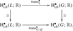
Here, the vertical arrows are the canonical isomorphisms obtained by extending the identity $\mathbb {R} \rightarrow \mathbb {R}$
to the complex of continuous bounded and essentially bounded functions, respectively.
$\mathbb {R} \rightarrow \mathbb {R}$
to the complex of continuous bounded and essentially bounded functions, respectively.
3 Pullback maps, multiplicative constants, and maximal measurable cocycles
The main goal of this section is to define pullbacks in continuous bounded cohomology via measurable cocycles and generalized boundary maps. As an application, we extend Burger and Iozzi’s useful formula for representations [Reference Burger and IozziBI09, Proposition 2.44] to the wider setting of measurable cocycles. This allows us to introduce the notion of multiplicative constants and investigate the rigidity of cocycles.
Setup 3.1. Let us consider the following setting:
-
• G is a second countable locally compact group;
-
•
$G'$
is a locally compact group which acts measurably on a measure space
$(Y, \nu )$
by preserving the measure class; -
• Q is a closed amenable subgroup of G;
-
• L is a lattice in G;
-
•
$(X,\mu _X)$
is a standard Borel probability L-space; -
•
$\sigma \colon L \times X \rightarrow G'$
is a measurable cocycle with an essentially unique generalized boundary map
$\phi \colon G/Q \times X \rightarrow Y$
.


3.1 Pullback along measurable cocycles and generalized boundary maps
In this section, we introduce two different pullback maps in continuous bounded cohomology associated with a measurable cocycle. The first pullback will only depend on the measurable cocycle $\sigma $
. The second will be defined in terms of the generalized boundary map
$\sigma $
. The second will be defined in terms of the generalized boundary map $\phi $
. We will show that under suitable conditions, the two definitions agree (Lemma 3.14). Despite a priori the first definition might appear more natural, we will mainly exploit the second pullback in the study of the rigidity properties of measurable cocycles.
$\phi $
. We will show that under suitable conditions, the two definitions agree (Lemma 3.14). Despite a priori the first definition might appear more natural, we will mainly exploit the second pullback in the study of the rigidity properties of measurable cocycles.
Given a measurable cocycle $\sigma \colon L \times X \rightarrow G'$
, we define a pullback map from
$\sigma \colon L \times X \rightarrow G'$
, we define a pullback map from $\operatorname {\mathrm{C}}^{\bullet}_{cb}(G';\operatorname {\mathrm {\mathbb {R}}})^{G'}$
to
$\operatorname {\mathrm{C}}^{\bullet}_{cb}(G';\operatorname {\mathrm {\mathbb {R}}})^{G'}$
to $\operatorname {\mathrm{C}}^{\bullet}_b(L;\operatorname {\mathrm {\mathbb {R}}})^L$
as follows (compare with [Reference Moraschini and SaviniMS, Remark 14]).
$\operatorname {\mathrm{C}}^{\bullet}_b(L;\operatorname {\mathrm {\mathbb {R}}})^L$
as follows (compare with [Reference Moraschini and SaviniMS, Remark 14]).
Definition 3.2. In the situation of Setup 3.1, the pullback map induced by the measurable cocycle $\sigma $
is given by
$\sigma $
is given by
 $$ \begin{align*}\operatorname{\mathrm{C}}_b^{\bullet}(\sigma) \colon\! \operatorname{\mathrm{C}}^{\bullet}_{cb}(G';\operatorname{\mathrm{\mathbb{R}}}) \rightarrow \operatorname{\mathrm{C}}^{\bullet}_b(L;\operatorname{\mathrm{\mathbb{R}}}), \end{align*} $$
 $$ \begin{align*}\psi \mapsto \operatorname{\mathrm{C}}^{\bullet}_b(\sigma)(\psi)(\gamma_1,\ldots,\gamma_{\bullet+1}) := \int_X(\psi(\sigma(\gamma_1^{-1},x)^{-1}),\ldots,\sigma(\gamma_{\bullet+1}^{-1},x)^{-1})\,d\mu_X(x). \end{align*} $$
Remark 3.3. The previous formula takes inspiration both from Bader, Furman and Sauer’s result [Reference Bader, Furman and SauerBFS13a, Theorem 5.6] and Monod and Shalom’s cohomological induction for measurable cocycles associated with couplings [Reference Monod and ShalomMS06, §4.2].
Lemma 3.4. In the situation of Setup 3.1, the map $\operatorname {\mathrm{C}}^{\bullet}_b(\sigma )$
is a well-defined cochain map which restricts to the subcomplexes of invariant cochains. Hence,
$\operatorname {\mathrm{C}}^{\bullet}_b(\sigma )$
is a well-defined cochain map which restricts to the subcomplexes of invariant cochains. Hence, $\operatorname {\mathrm{C}}^{\bullet}_b(\sigma )$
induces a map in bounded cohomology
$\operatorname {\mathrm{C}}^{\bullet}_b(\sigma )$
induces a map in bounded cohomology
 $$ \begin{align*}\operatorname{\mathrm{H}}^{\bullet}_b(\sigma):\operatorname{\mathrm{H}}^{\bullet}_{cb}(G';\operatorname{\mathrm{\mathbb{R}}}) \rightarrow \operatorname{\mathrm{H}}^{\bullet}_b(L;\operatorname{\mathrm{\mathbb{R}}}), \ \operatorname{\mathrm{H}}^{\bullet}_b(\sigma)([\psi]):=[ \operatorname{\mathrm{C}}^{\bullet}_b(\sigma)(\psi) ]. \end{align*} $$
Proof It is easy to check that $\operatorname {\mathrm{C}}^{\bullet}_b(\sigma )$
is a cochain map. Moreover, it sends bounded cochains to bounded cochains because
$\operatorname {\mathrm{C}}^{\bullet}_b(\sigma )$
is a cochain map. Moreover, it sends bounded cochains to bounded cochains because $\mu _X$
is a probability measure.
$\mu _X$
is a probability measure.
It only remains to prove that $\operatorname {\mathrm{C}}^{\bullet}_b(\sigma )$
sends
$\operatorname {\mathrm{C}}^{\bullet}_b(\sigma )$
sends $G'$
-invariant continuous cochains to L-invariant ones. Let
$G'$
-invariant continuous cochains to L-invariant ones. Let $\psi \in \operatorname {\mathrm{C}}^{\bullet}_{cb}(G';\operatorname {\mathrm {\mathbb {R}}})^{G'}$
and
$\psi \in \operatorname {\mathrm{C}}^{\bullet}_{cb}(G';\operatorname {\mathrm {\mathbb {R}}})^{G'}$
and $\gamma ,\gamma _1,\ldots ,\gamma _{\bullet+1} \in L$
, then we have
$\gamma ,\gamma _1,\ldots ,\gamma _{\bullet+1} \in L$
, then we have
 $$ \begin{align*} &\gamma \cdot \operatorname{\mathrm{C}}^{\bullet}_b(\sigma)(\psi)(\gamma_1,\ldots,\gamma_{\bullet+1})\\[-2pt] &\quad\qquad=\operatorname{\mathrm{C}}^{\bullet}_b(\sigma)(\psi)(\gamma^{-1}\gamma_1,\ldots,\gamma^{-1}\gamma_{\bullet+1})\\[-2pt] &\quad\qquad=\int_X \psi(\sigma(\gamma^{-1}_1 \gamma,x)^{-1},\ldots,\sigma(\gamma^{-1}_{\bullet+1} \gamma,x)^{-1})\,d\mu_X(x)\\[-2pt] &\quad\qquad=\int_X \psi(\sigma(\gamma,x)^{-1}\sigma(\gamma^{-1}_1,\gamma.x)^{-1},\ldots,\sigma(\gamma,x)^{-1}\sigma(\gamma_{\bullet+1}^{-1},\gamma.x)^{-1})\,d\mu_X(x)\\[-2pt] &\quad\qquad=\int_X \psi(\sigma(\gamma,x)^{-1}\sigma(\gamma^{-1}_1,x)^{-1},\ldots,\sigma(\gamma,x)^{-1}\sigma(\gamma_{\bullet+1}^{-1},x)^{-1})\,d\mu_X(x)\\[-2pt] &\quad\qquad=\int_X\psi(\sigma(\gamma^{-1}_1,x)^{-1},\ldots,\sigma(\gamma_{\bullet+1}^{-1},x)^{-1})\,d\mu_X(x)\\[-2pt] &\quad\qquad=\operatorname{\mathrm{C}}^{\bullet}_b(\sigma)(\psi)(\gamma_1,\ldots,\gamma_{\bullet+1}), \end{align*} $$
where the second line is equal to the third one because of the definition of a measurable cocycle (Equation (1)). Then, the L-invariance of the measure $\mu _X$
shows that the third line is equal to the fourth one. Finally, the
$\mu _X$
shows that the third line is equal to the fourth one. Finally, the $G'$
-invariance of
$G'$
-invariance of $\psi $
concludes the computation.
$\psi $
concludes the computation.
As anticipated, we now explain how to define a different pullback map via generalized boundary maps in the situation of Setup 3.1. This approach takes inspiration from a work by Bader, Furman, and Sauer [Reference Bader, Furman and SauerBFS13b, Proposition 4.2] and has already produced some applications in special settings (§3.5). We define the pullback along a generalized boundary map as the composition of two different maps defined in continuous bounded cohomology. The Banach space $\mathrm{L}^\infty (X) := \mathrm{L}^\infty (X; \mathbb {R})$
has a natural structure of Banach L-module given by the following L-action:
$\mathrm{L}^\infty (X) := \mathrm{L}^\infty (X; \mathbb {R})$
has a natural structure of Banach L-module given by the following L-action:
 $$ \begin{align*}\gamma.f = f(\gamma^{-1}.x), \end{align*} $$
for all $\gamma \in L$
and
$\gamma \in L$
and $f \in \, \operatorname {\mathrm{L}}^\infty (X)$
. This leads to the following.
$f \in \, \operatorname {\mathrm{L}}^\infty (X)$
. This leads to the following.
Definition 3.5. In the situation of Setup 3.1, the $\operatorname {\mathrm{L}}^\infty (X)$
-pullback along
$\operatorname {\mathrm{L}}^\infty (X)$
-pullback along $\phi $
is the following map:
$\phi $
is the following map:
 $$ \begin{align*}\operatorname{\mathrm{C}}^{\bullet}(\phi) \colon \mathcal{B}^\infty(Y^{\bullet + 1}; \mathbb{R})^{G'} \rightarrow \mathrm{L}_{\mathrm{w}^*}^\infty((G/Q)^{\bullet+1}; \operatorname{\mathrm{L}}^\infty(X))^L, \end{align*} $$
 $$ \begin{align*}\operatorname{\mathrm{C}}^{\bullet}(\phi)(\psi) (\eta_1, \ldots, \eta_{\bullet+1}) := (x \mapsto \psi(\phi(\eta_1, x), \ldots, \phi(\eta_{\bullet+1}, x))), \end{align*} $$
where $\psi \in \, \mathcal {B}^\infty (Y^{\bullet + 1}; \mathbb {R})^{G'}$
,
$\psi \in \, \mathcal {B}^\infty (Y^{\bullet + 1}; \mathbb {R})^{G'}$
, $\eta _1, \ldots , \eta _{\bullet+1} \in \, G/Q$
and
$\eta _1, \ldots , \eta _{\bullet+1} \in \, G/Q$
and $x \in \, X$
.
$x \in \, X$
.
Lemma 3.6. The map $\operatorname {\mathrm{C}}^{\bullet}(\phi )$
is a well-defined norm non-increasing cochain map.
$\operatorname {\mathrm{C}}^{\bullet}(\phi )$
is a well-defined norm non-increasing cochain map.
Proof Since $\operatorname {\mathrm{C}}^{\bullet}(\phi )$
is defined as a pullback, it is immediate to check that it is a norm non-increasing cochain map.
$\operatorname {\mathrm{C}}^{\bullet}(\phi )$
is defined as a pullback, it is immediate to check that it is a norm non-increasing cochain map.
Let us show now that for every $\psi \in \, \mathcal {B}^\infty (Y^{\bullet + 1}; \mathbb {R})^{G'}$
, the cocycle
$\psi \in \, \mathcal {B}^\infty (Y^{\bullet + 1}; \mathbb {R})^{G'}$
, the cocycle $\operatorname {\mathrm{C}}^{\bullet}(\phi )(\psi )$
is L-invariant. First, by [Reference MonodMon01, Corollary 2.3.3], we can identify
$\operatorname {\mathrm{C}}^{\bullet}(\phi )(\psi )$
is L-invariant. First, by [Reference MonodMon01, Corollary 2.3.3], we can identify
 $$ \begin{align*}\mathrm{L}_{\mathrm{w}^*}^\infty((G/Q)^{\bullet+1}; \operatorname{\mathrm{L}}^\infty(X))^L \cong \mathrm{L}^\infty((G/Q)^{\bullet+1} \times X)^L, \end{align*} $$
where the latter space is endowed with its natural diagonal L-action. Then, for almost every $x \in \, X$
,
$x \in \, X$
, $\gamma \in \, L$
, and
$\gamma \in \, L$
, and $\eta _1, \ldots , \eta _{\bullet+1} \in \, G/ Q$
, we have
$\eta _1, \ldots , \eta _{\bullet+1} \in \, G/ Q$
, we have
 $$ \begin{align*} \gamma \cdot \operatorname{\mathrm{C}}^{\bullet}(\phi)(\psi)(\eta_1, \ldots, \eta_{\bullet+1}) (x) &= \operatorname{\mathrm{C}}^{\bullet}(\phi)(\psi)(\gamma^{-1}.\eta_1,\ldots,\gamma^{-1}. \eta_{\bullet+1})(\gamma^{-1}.x)\\[-2pt] &=\psi(\phi(\gamma^{-1}.\eta_1, \gamma^{-1}.x), \ldots, \phi(\gamma^{-1}. \eta_{\bullet+1},\gamma^{-1}.x)) \\[-2pt] &= \psi(\sigma(\gamma^{-1}, x) \phi(\eta_1, x), \ldots, \sigma(\gamma^{-1}, x) \phi(\eta_{\bullet+1}, x))\\[-2pt] &= \psi(\phi(\eta_1, x), \ldots, \phi(\eta_{\bullet+1}, x)) \\[-2pt] &= \operatorname{\mathrm{C}}^{\bullet}(\phi)(\psi)(\eta_1, \ldots, \eta_{\bullet+1}) (x). \end{align*} $$
Here, we first used the definition of diagonal action, then the $\sigma $
-equivariance of
$\sigma $
-equivariance of $\phi $
, and finally the
$\phi $
, and finally the $G'$
-invariance of
$G'$
-invariance of $\psi $
.
$\psi $
.
Since our final goal is to pullback a cocycle $\psi \in \, \mathcal {B}^\infty (Y^{\bullet + 1}; \mathbb {R})^{G'}$
along
$\psi \in \, \mathcal {B}^\infty (Y^{\bullet + 1}; \mathbb {R})^{G'}$
along $\phi $
obtaining a new cocycle in
$\phi $
obtaining a new cocycle in $\mathrm{L}^\infty ((G/ Q)^{\bullet+1}; \mathbb {R})^L$
, we need to compose the
$\mathrm{L}^\infty ((G/ Q)^{\bullet+1}; \mathbb {R})^L$
, we need to compose the $\operatorname {\mathrm{L}}^\infty (X)$
-pullback along
$\operatorname {\mathrm{L}}^\infty (X)$
-pullback along $\phi $
with the integration map (compare with [Reference Bader, Furman and SauerBFS13b, Reference Moraschini and SaviniMS, Reference SaviniSava]).
$\phi $
with the integration map (compare with [Reference Bader, Furman and SauerBFS13b, Reference Moraschini and SaviniMS, Reference SaviniSava]).
Definition 3.7. In the situation of Setup 3.1, the integration map $\operatorname {\mathrm{I}}_X^{\bullet}$
is the following cochain map:
$\operatorname {\mathrm{I}}_X^{\bullet}$
is the following cochain map:
 $$ \begin{align*}\operatorname{\mathrm{I}}_X^{\bullet} \colon \mathrm{L}_{\mathrm{w}^*}^\infty((G/Q)^{\bullet+1}; \operatorname{\mathrm{L}}^\infty(X))^L \rightarrow \mathrm{L}^\infty((G/Q)^{\bullet+1}; \mathbb{R})^L, \\ \end{align*} $$
 $$ \begin{align*}\operatorname{\mathrm{I}}_X^{\bullet}(\psi)(\eta_1,\ldots,\eta_{\bullet+1}) := \int_X \psi(\eta_1, \ldots, \eta_{\bullet+1})(x)\, d\mu_X(x), \end{align*} $$
where $\psi \in \, \mathrm{L}^\infty ((G/Q)^{\bullet+1}; \operatorname {\mathrm{L}}^\infty (X))^L$
,
$\psi \in \, \mathrm{L}^\infty ((G/Q)^{\bullet+1}; \operatorname {\mathrm{L}}^\infty (X))^L$
, $\eta _1, \ldots , \eta _{\bullet+1} \in \, G/Q$
, and
$\eta _1, \ldots , \eta _{\bullet+1} \in \, G/Q$
, and $\mu _X$
is the probability measure on the standard Borel probability L-space X.
$\mu _X$
is the probability measure on the standard Borel probability L-space X.
Lemma 3.8. The integration map $\operatorname {\mathrm{I}}^{\bullet}_X$
is a well-defined norm non-increasing cochain map.
$\operatorname {\mathrm{I}}^{\bullet}_X$
is a well-defined norm non-increasing cochain map.
Proof Given a cocycle $\psi \in \, \mathrm{L}_{\mathrm{w}^*}^\infty ((G/Q)^{\bullet+1}; \operatorname {\mathrm{L}}^\infty (X))^L$
, it is easy to show that
$\psi \in \, \mathrm{L}_{\mathrm{w}^*}^\infty ((G/Q)^{\bullet+1}; \operatorname {\mathrm{L}}^\infty (X))^L$
, it is easy to show that $\operatorname {\mathrm{I}}^{\bullet}_X(\psi )$
is L-invariant. Indeed, given
$\operatorname {\mathrm{I}}^{\bullet}_X(\psi )$
is L-invariant. Indeed, given $\eta _1,\ldots ,\eta _{\bullet+1} \in G/Q$
and
$\eta _1,\ldots ,\eta _{\bullet+1} \in G/Q$
and $\gamma \in \, L$
, we have
$\gamma \in \, L$
, we have
 $$ \begin{align*} \gamma. \operatorname{\mathrm{I}}_X^{\bullet}(\psi)(\eta_1, \ldots, \eta_{\bullet+1}) &= \int_X \psi(\gamma^{-1}.\eta_1, \ldots, \gamma^{-1}. \eta_{\bullet+1})(x)\, d\mu_X(x)\\[5pt] &= \int_X \psi(\eta_1, \ldots, \eta_{\bullet+1})(\gamma.x)\, d\mu_X(x) \\[5pt] &= \int_X \psi(\eta_1, \ldots, \eta_{\bullet+1})(x)\, d\mu_X(x) = \operatorname{\mathrm{I}}^{\bullet}_X(\psi)(\eta_1, \ldots, \eta_{\bullet+1}), \end{align*} $$
where we used the L-invariance of both $\psi $
and
$\psi $
and $\mu _X$
.
$\mu _X$
.
Since it is immediate to check that the integration map is also a norm non-increasing cochain map, we get the thesis.
Remark 3.9. The previous construction via integration is only possible working with bounded cocycles. Indeed, there is no hope to extend this map to the case of unbounded cochains [Reference Moraschini and SaviniMS, Remarks 13 and 16].
We are now ready to define the pullback map along $\phi $
.
$\phi $
.
Definition 3.10. In the situation of Setup 3.1, the pullback map along the (generalized) boundary map $\phi $
is the following cochain map:
$\phi $
is the following cochain map:
 $$ \begin{align*}\operatorname{\mathrm{C}}^{\bullet}(\Phi^X) \colon \mathcal{B}^\infty(Y^{\bullet + 1}; \mathbb{R})^{G'} \rightarrow \mathrm{L}^\infty((G/Q)^{\bullet+1}; \mathbb{R})^L, \end{align*} $$
 $$ \begin{align*}\operatorname{\mathrm{C}}^{\bullet}(\Phi^X) := \operatorname{\mathrm{I}}^{\bullet}_X \circ \operatorname{\mathrm{C}}^{\bullet}(\phi). \end{align*} $$
Remark 3.11. The restriction of the pullback along $\phi $
to the subcomplexes of alternating cochains (Definition 2.27) is well defined.
$\phi $
to the subcomplexes of alternating cochains (Definition 2.27) is well defined.
The fact that the pullback map induces a well-defined map in cohomology is proved in the following.
Proposition 3.12. In the situation of Setup 3.1, the pullback map $\operatorname {\mathrm{C}}^{\bullet}(\Phi ^X)$
is a norm non-increasing cochain map. Hence, it induces a well-defined map
$\operatorname {\mathrm{C}}^{\bullet}(\Phi ^X)$
is a norm non-increasing cochain map. Hence, it induces a well-defined map
 $$ \begin{align*}\operatorname{\mathrm{H}}^{\bullet}(\Phi^X) \colon\! \operatorname{\mathrm{H}}^{\bullet}(\operatorname{\mathrm{\mathcal{B}}}^\infty(Y^{\bullet+1};\operatorname{\mathrm{\mathbb{R}}})^{G'}) \rightarrow \operatorname{\mathrm{H}}^{\bullet}_{b}(L;\operatorname{\mathrm{\mathbb{R}}}), \quad \operatorname{\mathrm{H}}^{\bullet}(\Phi^X)([\psi]):=[\operatorname{\mathrm{C}}^{\bullet}(\Phi^X)(\psi)]. \end{align*} $$
The same result still holds for the subcomplexes of alternating cochains.
Proof As a consequence of both Lemmas 3.6 and 3.8, the pullback $\operatorname {\mathrm{C}}^{\bullet}(\Phi ^X)$
is a norm non-increasing cochain map. Indeed, it is the composition of two such maps, namely
$\operatorname {\mathrm{C}}^{\bullet}(\Phi ^X)$
is a norm non-increasing cochain map. Indeed, it is the composition of two such maps, namely $\operatorname {\mathrm{C}}^{\bullet}(\phi )$
and
$\operatorname {\mathrm{C}}^{\bullet}(\phi )$
and $\operatorname {\mathrm{I}}^{\bullet}_X$
.
$\operatorname {\mathrm{I}}^{\bullet}_X$
.
Since Q is an amenable group, then $G/ Q$
is an amenable regular G-space (Example 2.5.2 and Remark 2.7). Hence, by Remark 2.29, the complex of L-invariant essentially bounded functions
$G/ Q$
is an amenable regular G-space (Example 2.5.2 and Remark 2.7). Hence, by Remark 2.29, the complex of L-invariant essentially bounded functions $\operatorname {\mathrm{L}}^\infty ((G/Q)^{\bullet+1};\operatorname {\mathrm {\mathbb {R}}})^L$
computes the continuous bounded cohomology
$\operatorname {\mathrm{L}}^\infty ((G/Q)^{\bullet+1};\operatorname {\mathrm {\mathbb {R}}})^L$
computes the continuous bounded cohomology $\operatorname {\mathrm{H}}^{\bullet}_{b}(L;\operatorname {\mathrm {\mathbb {R}}})$
.
$\operatorname {\mathrm{H}}^{\bullet}_{b}(L;\operatorname {\mathrm {\mathbb {R}}})$
.
The same proof adapts mutatis mutandis to the case of alternating cochains.
Remark 3.13. One might define a pullback map in cohomology using any measurable $\sigma $
-equivariant map
$\sigma $
-equivariant map $\phi \colon S \times X \rightarrow Y$
, where S is any amenable L-space. However, since we will not need this formulation in the following, we preferred to keep the previous setting.
$\phi \colon S \times X \rightarrow Y$
, where S is any amenable L-space. However, since we will not need this formulation in the following, we preferred to keep the previous setting.
Since we have introduced two different pullback maps in continuous bounded cohomology arising from measurable cocycles, it is natural to ask whether they agree. The following lemma completely describes the situation (compare with [Reference Burger, Iozzi, Burger and MonodBI02, Corollary 2.7]).
Lemma 3.14. In the situation of Setup 3.1, let $\psi \in \operatorname {\mathrm {\mathcal {B}}}^\infty (Y^{\bullet+1};\operatorname {\mathrm {\mathbb {R}}})^{G'}$
be a measurable cocycle. Then
$\psi \in \operatorname {\mathrm {\mathcal {B}}}^\infty (Y^{\bullet+1};\operatorname {\mathrm {\mathbb {R}}})^{G'}$
be a measurable cocycle. Then
 $$ \begin{align*}\operatorname{\mathrm{C}}^{\bullet}(\Phi^X)(\psi) \in \operatorname{\mathrm{L}}^\infty((G/Q)^{\bullet+1};\operatorname{\mathrm{\mathbb{R}}})^L \end{align*} $$
is a representative of the class $\operatorname {\mathrm{H}}^{\bullet}_b(\sigma )([\psi ]) \in \operatorname {\mathrm{H}}^{\bullet}_{b}(L;\operatorname {\mathrm {\mathbb {R}}})$
.
$\operatorname {\mathrm{H}}^{\bullet}_b(\sigma )([\psi ]) \in \operatorname {\mathrm{H}}^{\bullet}_{b}(L;\operatorname {\mathrm {\mathbb {R}}})$
.
Proof It is sufficient to consider the following commutative diagram [Reference Burger, Iozzi, Burger and MonodBI02, Proposition 1.2]:

where $\mathfrak{c}^{\bullet}$
is the map introduced in equation (3).
$\mathfrak{c}^{\bullet}$
is the map introduced in equation (3).
Finally, we show that the pullback along cohomologous measurable cocyles is the same (compare with [Reference Moraschini and SaviniMS, Propositions 13 and 20]).
Proposition 3.15. In the situation of Setup 3.1, let $f.\sigma \colon L \times X \rightarrow G'$
be a cocycle cohomologous to
$f.\sigma \colon L \times X \rightarrow G'$
be a cocycle cohomologous to $\sigma $
with respect to a measurable map
$\sigma $
with respect to a measurable map $f \colon X \rightarrow G'$
. Then, for every
$f \colon X \rightarrow G'$
. Then, for every $\psi \in \mathcal {B}^\infty (Y^{\bullet + 1}; \mathbb {R})^{G'}$
, we have
$\psi \in \mathcal {B}^\infty (Y^{\bullet + 1}; \mathbb {R})^{G'}$
, we have
 $$ \begin{align*}\operatorname{\mathrm{C}}^{\bullet}(\Phi^X)(\psi) = \operatorname{\mathrm{C}}^{\bullet}(f.\Phi^X)(\psi).\end{align*} $$
Here, $\operatorname {\mathrm{C}}^{\bullet}(\Phi ^X)$
and
$\operatorname {\mathrm{C}}^{\bullet}(\Phi ^X)$
and $\operatorname {\mathrm{C}}^{\bullet}(f.\Phi ^X)$
denote the pullback maps along the associated boundary maps
$\operatorname {\mathrm{C}}^{\bullet}(f.\Phi ^X)$
denote the pullback maps along the associated boundary maps $\phi $
and
$\phi $
and $f.\phi $
, respectively.
$f.\phi $
, respectively.
Proof The boundary map $f.\phi $
associated with
$f.\phi $
associated with $f.\sigma $
is given by
$f.\sigma $
is given by
 $$ \begin{align*}f.\phi \colon G/Q \times X \rightarrow Y, \hspace{10pt} (f.\phi)(\eta, x) = f^{-1}(x) \phi(\eta, x), \end{align*} $$
for almost every $\eta \in \, G/Q$
and
$\eta \in \, G/Q$
and $x \in \, X$
(Remark 2.13). Hence, we have
$x \in \, X$
(Remark 2.13). Hence, we have
 $$ \begin{align*} \operatorname{\mathrm{C}}^{\bullet}(f.\Phi^X)(\psi)(\eta_1, \ldots, \eta_{\bullet+1}) &= \int_X \psi((f.\phi)(\eta_1, x), \ldots, (f.\phi)(\eta_{\bullet +1}, x))\, d\mu_X(x) \\ &= \int_X \psi(f^{-1}(x) \phi(\eta_1, x), \ldots, f^{-1}(x) \phi(\eta_{\bullet +1}, x))\, d\mu_X(x) \\ &= \int_X \psi( \phi(\eta_1, x), \ldots, \phi(\eta_{\bullet +1}, x))\, d\mu_X(x) \\ &=\operatorname{\mathrm{C}}^{\bullet}(\Phi^X)(\psi)(\eta_1, \ldots, \eta_{\bullet+1}), \end{align*} $$
for almost every $\eta _1, \ldots , \eta _{\bullet +1 } \in \, G/Q$
. This finishes the proof.
$\eta _1, \ldots , \eta _{\bullet +1 } \in \, G/Q$
. This finishes the proof.
Remark 3.16. Sometimes it is natural to consider the $G'$
-module
$G'$
-module $\mathbb {R}$
with a twisted action. For instance, if
$\mathbb {R}$
with a twisted action. For instance, if $G'$
admits a sign homomorphism, we can use it to twist the real coefficients. In that situation, the previous equality will be true only up to a sign (see for instance [Reference Moraschini and SaviniMS, Proposition 13]).
$G'$
admits a sign homomorphism, we can use it to twist the real coefficients. In that situation, the previous equality will be true only up to a sign (see for instance [Reference Moraschini and SaviniMS, Proposition 13]).
3.2 Pullback along generalized boundary maps vs. pullback of representations
In the situation of Setup 3.1, let $(X,\mu _X)$
be a standard Borel probability L-space and let
$(X,\mu _X)$
be a standard Borel probability L-space and let $\rho \colon L \rightarrow G'$
be a representation. Then, there exists an associated measurable cocycle
$\rho \colon L \rightarrow G'$
be a representation. Then, there exists an associated measurable cocycle $\sigma _\rho \colon L \times X \rightarrow G'$
defined by
$\sigma _\rho \colon L \times X \rightarrow G'$
defined by $\sigma _\rho (\gamma , x) = \rho (\gamma )$
for every
$\sigma _\rho (\gamma , x) = \rho (\gamma )$
for every $\gamma \in \, L$
and
$\gamma \in \, L$
and $x \in \, X$
(Definition 2.14). If
$x \in \, X$
(Definition 2.14). If $\rho $
admits a
$\rho $
admits a $\rho $
-equivariant measurable map
$\rho $
-equivariant measurable map $\varphi \colon G/Q \rightarrow Y$
, the corresponding generalized boundary map of
$\varphi \colon G/Q \rightarrow Y$
, the corresponding generalized boundary map of $\sigma _\rho $
is
$\sigma _\rho $
is
 $$ \begin{align*}\phi \colon G/Q \times X \rightarrow Y, \quad \phi(\eta, x) = \varphi(\eta), \end{align*} $$
for almost every $\eta \in \, G/Q$
and
$\eta \in \, G/Q$
and $x \in \, X$
.
$x \in \, X$
.
As explained by Burger and Iozzi [Reference Burger, Iozzi, Burger and MonodBI02, Reference Burger and IozziBI09], one can implement the pullback map
 $$ \begin{align*}\operatorname{\mathrm{H}}^{\bullet}_{cb}(\rho) \colon\! \operatorname{\mathrm{H}}^{\bullet}_{cb}(G'; \mathbb{R}) \rightarrow \operatorname{\mathrm{H}}^{\bullet}_{b}(L; \mathbb{R})\end{align*} $$
using a cochain map $\operatorname {\mathrm{C}}^{\bullet}(\varphi )$
defined by
$\operatorname {\mathrm{C}}^{\bullet}(\varphi )$
defined by
 $$ \begin{align*}\operatorname{\mathrm{C}}^{\bullet}(\varphi):\operatorname{\mathrm{\mathcal{B}}}^\infty(Y^{\bullet+1};\operatorname{\mathrm{\mathbb{R}}})^{G'} \rightarrow \operatorname{\mathrm{L}}^\infty((G/Q)^{\bullet+1};\operatorname{\mathrm{\mathbb{R}}})^L, \end{align*} $$
 $$ \begin{align*}\psi \mapsto \operatorname{\mathrm{C}}^{\bullet}(\varphi)(\psi)(\eta_1,\ldots,\eta_{\bullet+1}):=\psi(\varphi(\eta_1),\ldots,\varphi(\eta_{\bullet+1})), \end{align*} $$
for almost every $\eta _1,\ldots ,\eta _{\bullet+1} \in G/Q$
.
$\eta _1,\ldots ,\eta _{\bullet+1} \in G/Q$
.
The following result shows that the pullback associated with $\rho $
via
$\rho $
via $\varphi $
agrees with the one along
$\varphi $
agrees with the one along $\phi $
. This property turns out to be fundamental to coherently extend the numerical invariants of representations to those of measurable cocycles (see [Reference SaviniSava, Proposition 3.4] and [Reference Moraschini and SaviniMS, Propositions 12 and 19]).
$\phi $
. This property turns out to be fundamental to coherently extend the numerical invariants of representations to those of measurable cocycles (see [Reference SaviniSava, Proposition 3.4] and [Reference Moraschini and SaviniMS, Propositions 12 and 19]).
Proposition 3.17. In the situation of Setup 3.1, let $\rho \colon L \rightarrow G'$
be a representation which admits a
$\rho \colon L \rightarrow G'$
be a representation which admits a $\rho $
-equivariant measurable map
$\rho $
-equivariant measurable map $\varphi \colon G/Q \rightarrow Y$
. Then, we have
$\varphi \colon G/Q \rightarrow Y$
. Then, we have
 $$ \begin{align*}\operatorname{\mathrm{C}}^{\bullet}(\Phi^X)=\operatorname{\mathrm{C}}^{\bullet}(\varphi). \end{align*} $$
Proof Since the boundary map $\phi $
associated with
$\phi $
associated with $\sigma _\rho $
does not depend on the second variable, it is immediate to check that the following diagram commutes:
$\sigma _\rho $
does not depend on the second variable, it is immediate to check that the following diagram commutes:

from which the thesis.
Remark 3.18. The existence of a cocycle of the form $\sigma \colon L \times X \rightarrow G'$
required in Setup 3.1 is irrelevant in the previous result.
$\sigma \colon L \times X \rightarrow G'$
required in Setup 3.1 is irrelevant in the previous result.
3.3 Multiplicative formula
In this section, we prove how to deduce the multiplicative formula stated in Proposition 1.1. Some applications of the formula are then discussed in §3.5.
Proposition 3.19. In the situation of Setup 3.1, let $\psi ' \in \operatorname {\mathrm {\mathcal {B}}}^\infty (Y^{\bullet+1};\operatorname {\mathrm {\mathbb {R}}})^{G'}$
be an every where-defined
$\psi ' \in \operatorname {\mathrm {\mathcal {B}}}^\infty (Y^{\bullet+1};\operatorname {\mathrm {\mathbb {R}}})^{G'}$
be an every where-defined $G'$
-invariant cocycle. Let
$G'$
-invariant cocycle. Let $\psi \in \operatorname {\mathrm{L}}^\infty ((G/Q)^{\bullet+1})^G$
be a G-invariant cocycle. Denote by
$\psi \in \operatorname {\mathrm{L}}^\infty ((G/Q)^{\bullet+1})^G$
be a G-invariant cocycle. Denote by $\Psi \in \operatorname {\mathrm{H}}^{\bullet}_{cb}(G;\operatorname {\mathrm {\mathbb {R}}})$
the class of
$\Psi \in \operatorname {\mathrm{H}}^{\bullet}_{cb}(G;\operatorname {\mathrm {\mathbb {R}}})$
the class of $\psi $
. Assume that
$\psi $
. Assume that $\Psi =\mathrm{trans}_{G/Q}^{\bullet} [\operatorname {\mathrm{C}}^{\bullet}(\Phi ^X)(\psi ')]$
.
$\Psi =\mathrm{trans}_{G/Q}^{\bullet} [\operatorname {\mathrm{C}}^{\bullet}(\Phi ^X)(\psi ')]$
.
-
(1) We have that
for almost every
$$ \begin{align*} &\int_{L \backslash G} \int_X \psi'(\phi(\overline{g}.\eta_1, x), \ldots, \phi(\overline{g}.\eta_{\bullet+1}, x)) d\mu_X(x)\, d\mu(\overline{g})\\ &\quad= \psi(\eta_1, \ldots, \eta_{\bullet+1}) + \mathrm{cobound.}, \end{align*} $$
$(\eta _1,\ldots ,\eta _{\bullet+1}) \in (G/Q)^{\bullet+1}$
.
-
(2) If
$\operatorname {\mathrm{H}}^{\bullet}_{cb}(G;\operatorname {\mathrm {\mathbb {R}}}) \cong \operatorname {\mathrm {\mathbb {R}}} \Psi (= \operatorname {\mathrm {\mathbb {R}}}[\psi ])$
, then there exists a real constant
$\lambda _{\psi ',\psi }(\sigma ) \in \operatorname {\mathrm {\mathbb {R}}}$
depending on
$\sigma ,\psi ',\psi $
such that for almost every
$$ \begin{align*} &\int_{L\backslash G} \int_X \psi'(\phi(\overline{g}.\eta_1, x), \ldots, \phi(\overline{g}.\eta_{\bullet+1}, x)) d\mu_X(x)\, d\mu(\overline{g})\\ &\quad=\lambda_{\psi',\psi}(\sigma) \cdot \psi(\eta_1,\ldots,\eta_{\bullet+1}) +\mathrm{cobound.}, \end{align*} $$
$(\eta _1,\ldots ,\eta _{\bullet+1}) \in (G/Q)^{\bullet+1}$
.
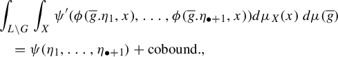


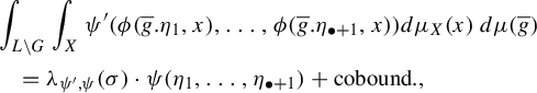

Proof
Ad 1. Since Setup 3.1 ensures the existence of the transfer map $\operatorname {\mathrm {trans}}_{G/Q}^{\bullet}$
, the first formula is easily true.
$\operatorname {\mathrm {trans}}_{G/Q}^{\bullet}$
, the first formula is easily true.
Ad 2. Since $\operatorname {\mathrm{H}}^{\bullet}_{cb}(G;\operatorname {\mathrm {\mathbb {R}}})$
is one-dimensional and generated by
$\operatorname {\mathrm{H}}^{\bullet}_{cb}(G;\operatorname {\mathrm {\mathbb {R}}})$
is one-dimensional and generated by $\Psi = [\psi ]$
as an
$\Psi = [\psi ]$
as an $\mathbb {R}$
-vector space,
$\mathbb {R}$
-vector space, $\mathrm{trans}_{G/Q}^{\bullet} [\operatorname {\mathrm{C}}^{\bullet}(\Phi ^X)(\psi ')]$
must be a real multiple of
$\mathrm{trans}_{G/Q}^{\bullet} [\operatorname {\mathrm{C}}^{\bullet}(\Phi ^X)(\psi ')]$
must be a real multiple of $\Psi $
. This finishes the proof.
$\Psi $
. This finishes the proof.
Remark 3.20.
A priori Proposition 1.1.2 only holds almost everywhere. However, as proved by Monod [Reference MonodMon15, §1.C], working with $\mathrm{L}^\infty $
-cocycles on Furstenberg–Poisson boundaries, one can always show that the previous formula holds everywhere [Reference MonodMon15, Theorem B] (compare with [Reference Bucher, Burger, Iozzi and PicardelloBBI13, §4]). We will use this fact in the proof of Theorem 3.28 in order to evaluate the formula at a given point.
$\mathrm{L}^\infty $
-cocycles on Furstenberg–Poisson boundaries, one can always show that the previous formula holds everywhere [Reference MonodMon15, Theorem B] (compare with [Reference Bucher, Burger, Iozzi and PicardelloBBI13, §4]). We will use this fact in the proof of Theorem 3.28 in order to evaluate the formula at a given point.
3.4 Multiplicative constants and maximal measurable cocycles
In this section, we are going to introduce the notion of a multiplicative constant. This definition will allow us to introduce maximal (measurable) cocycles and to investigate their rigidity properties.
In the situation of Setup 3.1, let $\psi ' \in \operatorname {\mathrm {\mathcal {B}}}^\infty (Y^{\bullet+1};\operatorname {\mathrm {\mathbb {R}}})^{G'}$
and let
$\psi ' \in \operatorname {\mathrm {\mathcal {B}}}^\infty (Y^{\bullet+1};\operatorname {\mathrm {\mathbb {R}}})^{G'}$
and let $\Psi =[\psi ] \in \operatorname {\mathrm{H}}^{\bullet}_{cb}(G;\operatorname {\mathrm {\mathbb {R}}})$
be represented by a bounded Borel cocycle
$\Psi =[\psi ] \in \operatorname {\mathrm{H}}^{\bullet}_{cb}(G;\operatorname {\mathrm {\mathbb {R}}})$
be represented by a bounded Borel cocycle $\psi \colon (G/Q)^{\bullet+1} \rightarrow \operatorname {\mathrm {\mathbb {R}}}$
. If
$\psi \colon (G/Q)^{\bullet+1} \rightarrow \operatorname {\mathrm {\mathbb {R}}}$
. If $\operatorname {\mathrm{H}}^{\bullet}_{cb}(G;\operatorname {\mathrm {\mathbb {R}}})=\operatorname {\mathrm {\mathbb {R}}} \Psi $
, then Proposition 1.1 implies
$\operatorname {\mathrm{H}}^{\bullet}_{cb}(G;\operatorname {\mathrm {\mathbb {R}}})=\operatorname {\mathrm {\mathbb {R}}} \Psi $
, then Proposition 1.1 implies
 $$ \begin{align} &\int_{L \backslash G} \int_X \psi'(\phi(\overline{g}.\eta_1,x),\ldots,\phi(\overline{g}.\eta_{\bullet+1},x))\,d\mu_X(x)\,d\mu(\overline{g})\nonumber\\ &\quad=\lambda_{\psi',\psi}(\sigma)\psi(\eta_1,\ldots,\eta_{\bullet+1}) + \mathrm{cobound}. \end{align} $$
Definition 3.21. The real number $\lambda _{\psi ',\psi }(\sigma ) \in \operatorname {\mathrm {\mathbb {R}}}$
appearing in equation (5) is the multiplicative constant associated with
$\lambda _{\psi ',\psi }(\sigma ) \in \operatorname {\mathrm {\mathbb {R}}}$
appearing in equation (5) is the multiplicative constant associated with $\sigma , \psi ', \psi $
.
$\sigma , \psi ', \psi $
.
A particularly nice situation for the study of rigidity phenomena is when, in equation (5), there are no coboundary terms. For this reason, we are going to introduce the following notation.
Definition 3.22. We say that condition $(\operatorname {\mathrm {\mbox {NCT}}})$
(no coboundary terms) is satisfied when equation (5) reduces to
$(\operatorname {\mathrm {\mbox {NCT}}})$
(no coboundary terms) is satisfied when equation (5) reduces to
 $$ \begin{align*} &\int_{L \backslash G} \int_X \psi'(\phi(\overline{g}.\eta_1,x),\ldots,\phi(\overline{g}.\eta_{\bullet+1},x))\,d\mu_X(x)\,d\mu(\overline{g})W\\ &\quad=\lambda_{\psi',\psi}(\sigma)\psi(\eta_1,\ldots,\eta_{\bullet+1}). \end{align*} $$
Example 3.23. Standard examples in which condition $(\operatorname {\mathrm {\mbox {NCT}}})$
is satisfied are the following.
$(\operatorname {\mathrm {\mbox {NCT}}})$
is satisfied are the following.
-
(1) Given a torsion-free lattice
$L \leq G$
in a semisimple Lie group and a minimal parabolic subgroup
$P \leq G$
, L acts doubly ergodically on the Furstenberg–Poisson boundary
$G/P$
[Reference AlbuquerqueAlb99, Theorem 5.6]. Hence condition
$(\operatorname {\mathrm {\mbox {NCT}}})$
is satisfied in degree
$n=2$
for bounded alternating cochains. -
(2) In degree
$n \geq 3$
, if
$G=\mathrm{PO}(n,1)$
and
$G/Q=\operatorname {\mathrm {\mathbb {S}}}^{n-1}$
, condition
$(\operatorname {\mathrm {\mbox {NCT}}} )$
holds when we consider the real bounded cohomology twisted by the sign action [Reference Bucher, Burger, Iozzi and PicardelloBBI13, Lemma 2.2].


Remark 3.24. The condition $(\operatorname {\mathrm {\mbox {NCT}}})$
has the following equivalent reformulation via cochains:
$(\operatorname {\mathrm {\mbox {NCT}}})$
has the following equivalent reformulation via cochains:
 $$ \begin{align*}\widehat{\mathrm{trans}}^{\bullet}_{G/Q} \circ \operatorname{\mathrm{C}}^{\bullet}(\Phi^X)(\psi')=\lambda_{\psi',\psi}(\sigma)\psi. \end{align*} $$
If condition $(\operatorname {\mathrm {\mbox {NCT}}})$
is satisfied, then there exists an explicit upper bound for the multiplicative constant
$(\operatorname {\mathrm {\mbox {NCT}}})$
is satisfied, then there exists an explicit upper bound for the multiplicative constant $\lambda _{\psi ',\psi }(\sigma )$
.
$\lambda _{\psi ',\psi }(\sigma )$
.
Proposition 3.25. In the situation of Setup 3.1, let $\psi ' \in \operatorname {\mathrm {\mathcal {B}}}^\infty (Y^{\bullet+1};\operatorname {\mathrm {\mathbb {R}}})^{G'}$
and let
$\psi ' \in \operatorname {\mathrm {\mathcal {B}}}^\infty (Y^{\bullet+1};\operatorname {\mathrm {\mathbb {R}}})^{G'}$
and let $\Psi =[\psi ] \in \operatorname {\mathrm{H}}^{\bullet}_{cb}(G;\operatorname {\mathrm {\mathbb {R}}})$
be represented by a bounded Borel cocycle
$\Psi =[\psi ] \in \operatorname {\mathrm{H}}^{\bullet}_{cb}(G;\operatorname {\mathrm {\mathbb {R}}})$
be represented by a bounded Borel cocycle $\psi \colon (G/Q)^{\bullet+1} \rightarrow \operatorname {\mathrm {\mathbb {R}}}$
. If condition
$\psi \colon (G/Q)^{\bullet+1} \rightarrow \operatorname {\mathrm {\mathbb {R}}}$
. If condition $(\mathrm{NCT})$
is satisfied, then we have
$(\mathrm{NCT})$
is satisfied, then we have
 $$ \begin{align*}|\lambda_{\psi',\psi}(\sigma)| \leq \frac{\lVert \psi' \rVert_\infty}{\lVert \psi \rVert_\infty}. \end{align*} $$
Proof By Remark 3.24, we know that
 $$ \begin{align*}\widehat{\mathrm{trans}}^{\bullet}_{G/Q} \circ \operatorname{\mathrm{C}}^{\bullet}(\Phi^X)(\psi')=\lambda_{\psi',\psi}(\sigma)\psi. \end{align*} $$
Since by Proposition 3.12 $\widehat {\mathrm{trans}}^{\bullet}_{G/Q}$
and
$\widehat {\mathrm{trans}}^{\bullet}_{G/Q}$
and $\operatorname {\mathrm{C}}^{\bullet}(\Phi ^X)$
are norm non-increasing maps, the left-hand side admits the following estimate:
$\operatorname {\mathrm{C}}^{\bullet}(\Phi ^X)$
are norm non-increasing maps, the left-hand side admits the following estimate:
 $$ \begin{align*}\lVert \widehat{\mathrm{trans}}^{\bullet}_{G/Q} \circ \operatorname{\mathrm{C}}^{\bullet}(\Phi^X)(\psi') \rVert_\infty \leq \lVert \psi' \rVert_\infty . \end{align*} $$
Hence, we get
 $$ \begin{align*}|\lambda_{\psi',\psi}(\sigma)| \lVert \psi \rVert_\infty \leq \lVert \psi' \rVert_\infty, \end{align*} $$
as desired.
Using the previous upper bound, we introduce the following.
Definition 3.26. In the situation of Setup 3.1, assume that condition $(\operatorname {\mathrm {\mbox {NCT}}})$
is satisfied. We say that a measurable cocycle
$(\operatorname {\mathrm {\mbox {NCT}}})$
is satisfied. We say that a measurable cocycle $\sigma \colon L \times X \rightarrow G'$
is maximal if its multiplicative constant
$\sigma \colon L \times X \rightarrow G'$
is maximal if its multiplicative constant $\lambda _{\psi ',\psi }(\sigma )$
attains the maximum value:
$\lambda _{\psi ',\psi }(\sigma )$
attains the maximum value:
 $$ \begin{align*}\lambda_{\psi',\psi}(\sigma) = \frac{\lVert \psi' \rVert_\infty}{\lVert \psi \rVert_\infty}. \end{align*} $$
For every representation $\pi \colon G \to G'$
, we denote the restriction of
$\pi \colon G \to G'$
, we denote the restriction of $\pi $
to L as
$\pi $
to L as $\pi |_L \colon $ $L \to G'$
. We prove now that under suitable assumptions, maximal cocycles can be trivialized, that is, they are cohomologous to a suitable representation
$L \to G'$
. We prove now that under suitable assumptions, maximal cocycles can be trivialized, that is, they are cohomologous to a suitable representation $\pi |_L \colon L \rightarrow G'$
.
$\pi |_L \colon L \rightarrow G'$
.
Setup 3.27. In the situation of Setup 3.1, assume that condition $(\mathrm{NCT})$
is satisfied. We also assume the following.
$(\mathrm{NCT})$
is satisfied. We also assume the following.
-
• Both
$\psi '$
and
$\psi $
are defined everywhere and they attain their essential supremum. There exist
$\eta _1,\ldots ,\eta _{\bullet+1} \in G/Q$
and
$y_1,\ldots ,y_{\bullet+1} \in Y$
, such that
$$ \begin{align*}\psi'(y_1,\ldots,y_{\bullet+1})=\lVert \psi' \rVert_\infty \quad \mbox{ and } \quad \psi(\eta_1,\ldots,\eta_{\bullet+1})=\lVert \psi \rVert_\infty. \end{align*} $$
-
• A maximal map
$\varphi \colon G/Q \rightarrow Y$
is a measurable map, such that for almost every
$$ \begin{align*}\psi'(\varphi(g\eta_1),\ldots,\varphi(g\eta_{\bullet+1}))=\lVert \psi' \rVert_\infty, \end{align*} $$
$g \in G$
and for every
$\eta _1,\ldots ,\eta _{\bullet+1} \in G/Q$
, such that
$$ \begin{align*}\psi(\eta_1,\ldots,\eta_{\bullet+1})=\lVert \psi \rVert_\infty.\end{align*} $$
-
• There exists a continuous representation
$\pi \colon G \rightarrow G'$
and unique continuous
$\pi $
-equivariant map
$\Pi \colon G/Q \rightarrow Y$
, which satisfies the following. Given any maximal measurable map
$\varphi \colon G/Q \rightarrow Y$
, there exists a unique element
$g_\varphi ' \in G'$
, such that for almost every
$$ \begin{align*}\varphi(\eta)=g_\varphi '\Pi(\eta), \end{align*} $$
$\eta \in G/Q$
.
-
• The
$G'$
-pointwise stabilizer of the map
$\Pi $
is trivial, that is, the only element
$g' \in G'$
, such that
$g' \Pi (x) = \Pi (x)$
for all
$x \in \, G/Q$
is the neutral element of
$G'$
. We denote the previous stabilizer by
$\mathrm{Stab}_{G'}(\Pi )$
.


Theorem 3.28. In the situation of Setup 3.27, let $\pi |_L \colon L \to G'$
be the restriction of the representation
$\pi |_L \colon L \to G'$
be the restriction of the representation $\pi \colon G \to G'$
to L. If the measurable cocycle
$\pi \colon G \to G'$
to L. If the measurable cocycle $\sigma \colon L \times X \rightarrow G'$
is maximal, then
$\sigma \colon L \times X \rightarrow G'$
is maximal, then $\sigma $
is cohomologous to
$\sigma $
is cohomologous to $\pi |_L$
.
$\pi |_L$
.
Remark 3.29. More precisely, the theorem shows the existence of a measurable map $f \colon X \rightarrow G'$
, such that, for all
$f \colon X \rightarrow G'$
, such that, for all $\gamma \in L$
and almost every
$\gamma \in L$
and almost every $x \in X$
, we have
$x \in X$
, we have
 $$ \begin{align*}\pi |_L (\gamma)=f(\gamma.x)^{-1}\sigma(\gamma,x)f(x). \end{align*} $$
Proof Since the cocycle $\sigma $
is maximal, we know that
$\sigma $
is maximal, we know that
 $$ \begin{align*}\lambda_{\psi',\psi}(\sigma) = \frac{\lVert \psi' \rVert_\infty}{\lVert \psi \rVert_\infty}. \end{align*} $$
Under condition $(\operatorname {\mathrm {\mbox {NCT}}})$
, if we substitute the value of
$(\operatorname {\mathrm {\mbox {NCT}}})$
, if we substitute the value of $\lambda _{\psi ',\psi }(\sigma )$
in equation (5), we get
$\lambda _{\psi ',\psi }(\sigma )$
in equation (5), we get
 $$ \begin{align} \int_{L \backslash G} \int_X \psi'(\phi(\overline{g}.\eta_1,x),\ldots,\phi(\overline{g}.\eta_{\bullet+1},x))\,d\mu_X(x)\,d\mu(\overline{g})=\frac{\lVert \psi' \rVert_\infty}{\lVert \psi \rVert_\infty}\psi(\eta_1,\ldots,\eta_{\bullet+1}). \end{align} $$
Moreover, by assumption, $\psi $
attains its essential supremum, from which there exist
$\psi $
attains its essential supremum, from which there exist $\hat {\eta }_1,\ldots ,\hat {\eta }_{\bullet+1} \in G/Q$
, such that
$\hat {\eta }_1,\ldots ,\hat {\eta }_{\bullet+1} \in G/Q$
, such that
 $$ \begin{align} \psi(\hat{\eta}_1,\ldots,\hat{\eta}_{\bullet+1})=\lVert \psi \rVert_\infty. \end{align} $$
By Remark 3.20, we can evaluate equation (6) at $\hat {\eta }_1,\ldots ,\hat {\eta }_{\bullet+1} \in G/Q$
. Hence, by equation (7), we have
$\hat {\eta }_1,\ldots ,\hat {\eta }_{\bullet+1} \in G/Q$
. Hence, by equation (7), we have
 $$ \begin{align} \int_{L \backslash G} \int_X \psi'(\phi(\overline{g}.\hat{\eta}_1,x),\ldots,\phi(\overline{g}.\hat{\eta}_{\bullet+1},x))\,d\mu_X(x)\,d\mu(\overline{g})=\lVert \psi' \rVert_\infty. \end{align} $$
This shows that
 $$ \begin{align*}\psi'(\phi(\overline{g}.\hat{\eta}_1,x),\ldots,\phi(\overline{g}.\hat{\eta}_{\bullet+1},x))=\lVert \psi' \rVert_\infty \ , \end{align*} $$
for almost every $\overline {g} \in L \backslash G$
and almost every
$\overline {g} \in L \backslash G$
and almost every $x \in X$
. Additionally, the
$x \in X$
. Additionally, the $\sigma $
-equivariance of
$\sigma $
-equivariance of $\phi $
implies that, in fact,
$\phi $
implies that, in fact,
 $$ \begin{align} \psi'(\phi(g.\hat{\eta}_1,x),\ldots,\phi(g.\hat{\eta}_{\bullet+1},x))=\lVert \psi' \rVert_\infty \end{align} $$
holds for almost every $g \in G$
and almost every
$g \in G$
and almost every $x \in X$
.
$x \in X$
.
We can define for almost every $x \in \, X$
a map
$x \in \, X$
a map
 $$ \begin{align*}\phi_x \colon G/Q \rightarrow Y, \quad \phi_x(\eta):=\phi(\eta,x),\end{align*} $$
which is measurable [Reference Fisher, Morris and WhyteFMW04, Lemma 2.6] and maximal by equation (9). Hence, by the assumptions of Setup 3.27, for almost every $x \in X$
, there must exist an element
$x \in X$
, there must exist an element $g_x \in G'$
, such that
$g_x \in G'$
, such that
 $$ \begin{align*}\phi_x(\eta)=g_x\Pi(\eta), \end{align*} $$
for almost every $\eta \in G/Q$
. This shows that
$\eta \in G/Q$
. This shows that $\phi _x$
lies in the
$\phi _x$
lies in the $G'$
-orbit of
$G'$
-orbit of $\Pi $
. In this way, we get a map
$\Pi $
. In this way, we get a map
 $$ \begin{align*}\widehat{\phi} \colon X \rightarrow G'.\Pi, \quad\widehat{\phi}(x)=\phi_x, \end{align*} $$
which is measurable [Reference Fisher, Morris and WhyteFMW04, Lemma 2.6]. By Setup 3.27, the stabilizer of $\Pi $
is trivial and hence the orbit
$\Pi $
is trivial and hence the orbit $G'.\Pi $
is naturally homeomorphic to
$G'.\Pi $
is naturally homeomorphic to $G'$
through a map
$G'$
through a map $\jmath \colon G'.\Pi \rightarrow G'$
. Composing the identification
$\jmath \colon G'.\Pi \rightarrow G'$
. Composing the identification $\jmath $
with the map
$\jmath $
with the map $\widehat {\phi }$
, we get a map
$\widehat {\phi }$
, we get a map
 $$ \begin{align*}f \colon X \rightarrow G', \quad f(x):= (\jmath \circ \widehat{\phi})(x), \end{align*} $$
which is defined almost everywhere and it is measurable being the composition of measurable maps (notice that the composition above gives back the element $g_x$
).
$g_x$
).
We can now conclude the proof (compare with [Reference Bader, Furman and SauerBFS13b, Proposition 3.2]). Given $\gamma \in L$
, on the one hand, we have
$\gamma \in L$
, on the one hand, we have
 $$ \begin{align*}\phi(\gamma.\eta,\gamma.x)=\sigma(\gamma,x)\phi(\eta,x)=\sigma(\gamma,x)f(x)\Pi(\eta), \end{align*} $$
and on the other,
 $$ \begin{align*}\phi(\gamma.\eta,\gamma.x)=f(\gamma.x)\Pi(\gamma.x)=f(\gamma.x)\pi |_L (\gamma)\Pi(\eta). \end{align*} $$
In the second equality, we used the $\pi $
-equivariance of the map
$\pi $
-equivariance of the map $\Pi $
. The fact that
$\Pi $
. The fact that $\mathrm{Stab}_{G'}(\Pi )$
is trivial implies that
$\mathrm{Stab}_{G'}(\Pi )$
is trivial implies that
 $$ \begin{align*}\pi |_L (\gamma)=f(\gamma.x)^{-1}\sigma(\gamma,x)f(x), \end{align*} $$
which finishes the proof.
3.5 Applications of the multiplicative formula
For the convenience of the reader, we collect here some examples of applications of Proposition 1.1.
Example 3.30. Let $n \geq 3$
. Let
$n \geq 3$
. Let $L \leq G = \operatorname {\mathrm{PO}}^\circ (n, 1)$
be a torsion-free non-uniform lattice and
$L \leq G = \operatorname {\mathrm{PO}}^\circ (n, 1)$
be a torsion-free non-uniform lattice and $(X, \mu _X)$
be a standard Borel probability L-space. Following the notation of Setup 3.1, we set
$(X, \mu _X)$
be a standard Borel probability L-space. Following the notation of Setup 3.1, we set $G' = \operatorname {\mathrm{PO}}^\circ (n, 1)$
and
$G' = \operatorname {\mathrm{PO}}^\circ (n, 1)$
and $Y = G/Q = \partial \mathbb {H}^n_{\mathbb {R}} \cong \mathbb {S}^{n-1}$
, where Q is a (minimal) parabolic subgroup of G. Using bounded cohomology theory [Reference GromovGro82, Reference Frigerio and MoraschiniFM], one can define the volume
$Y = G/Q = \partial \mathbb {H}^n_{\mathbb {R}} \cong \mathbb {S}^{n-1}$
, where Q is a (minimal) parabolic subgroup of G. Using bounded cohomology theory [Reference GromovGro82, Reference Frigerio and MoraschiniFM], one can define the volume $\operatorname {\mathrm {Vol}}(\sigma )$
of a measurable cocycle
$\operatorname {\mathrm {Vol}}(\sigma )$
of a measurable cocycle $\sigma \colon L \times X \to \operatorname {\mathrm{PO}}^\circ (n,1)$
[Reference Moraschini and SaviniMS, §4.1]. As proved by the authors [Reference Moraschini and SaviniMS, Proposition 2], in this setting, the multiplicative constant is given by
$\sigma \colon L \times X \to \operatorname {\mathrm{PO}}^\circ (n,1)$
[Reference Moraschini and SaviniMS, §4.1]. As proved by the authors [Reference Moraschini and SaviniMS, Proposition 2], in this setting, the multiplicative constant is given by
 $$ \begin{align*}\lambda_{\psi', \psi}(\sigma) = \frac{\operatorname{\mathrm{Vol}}(\sigma)}{\operatorname{\mathrm{Vol}}(L \backslash \mathbb{H}^n)}. \end{align*} $$
Since condition $(\operatorname {\mathrm {\mbox {NCT}}})$
is satisfied for twisted real coefficients [Reference Bucher, Burger, Iozzi and PicardelloBBI13, Lemma 2.2], Proposition 3.25 shows that the following Milnor–Wood inequality holds [Reference Moraschini and SaviniMS, Proposition 15]:
$(\operatorname {\mathrm {\mbox {NCT}}})$
is satisfied for twisted real coefficients [Reference Bucher, Burger, Iozzi and PicardelloBBI13, Lemma 2.2], Proposition 3.25 shows that the following Milnor–Wood inequality holds [Reference Moraschini and SaviniMS, Proposition 15]:
 $$ \begin{align*}|\! \operatorname{\mathrm{Vol}}(\sigma) | \leq \operatorname{\mathrm{Vol}}(L \backslash \mathbb{H}^n). \end{align*} $$
Finally one can apply Theorem 3.28 to show that if $\sigma $
is maximal, then
$\sigma $
is maximal, then $\sigma $
is cohomologous to the cocycle associated with the standard lattice embedding
$\sigma $
is cohomologous to the cocycle associated with the standard lattice embedding $L \rightarrow G$
. In fact, one can strengthen this result. A cocycle is maximal if and only if it is cohomologous to the cocycle associated with the standard lattice embedding [Reference Moraschini and SaviniMS, Theorem 1].
$L \rightarrow G$
. In fact, one can strengthen this result. A cocycle is maximal if and only if it is cohomologous to the cocycle associated with the standard lattice embedding [Reference Moraschini and SaviniMS, Theorem 1].
Similarly, one can apply an analogous strategy for studying the case of closed surfaces. The main difference is that we have to to fix a hyperbolization. Then, maximal cocycles will be cohomologous to the given hyperbolization [Reference Moraschini and SaviniMS, Theorem 5].
Example 3.31. Fix a torsion-free lattice $L \leq G = \mathrm{PSL}(2,\mathbb {C})$
together with a standard Borel probability L-space
$L \leq G = \mathrm{PSL}(2,\mathbb {C})$
together with a standard Borel probability L-space $(X, \mu _X)$
. Following the notation of Setup 3.1, we set
$(X, \mu _X)$
. Following the notation of Setup 3.1, we set $G' = \mathrm{PSL}(n,\mathbb {C})$
,
$G' = \mathrm{PSL}(n,\mathbb {C})$
, $Y=\mathscr {F}(n,\mathbb {C})$
is the space of full flags, and
$Y=\mathscr {F}(n,\mathbb {C})$
is the space of full flags, and $G/Q = \mathbb {P}^1(\mathbb {C})$
. Here, Q is a (minimal) parabolic subgroup of G. The second author defined the Borel invariant
$G/Q = \mathbb {P}^1(\mathbb {C})$
. Here, Q is a (minimal) parabolic subgroup of G. The second author defined the Borel invariant $\beta _n(\sigma )$
of a measurable cocycle
$\beta _n(\sigma )$
of a measurable cocycle $\sigma \colon L \times X \to \mathrm{PSL}(n,\mathbb {C})$
[Reference SaviniSava, §4]. Then, the multiplicative constant is given by [Reference SaviniSava, Proposition 1.2]
$\sigma \colon L \times X \to \mathrm{PSL}(n,\mathbb {C})$
[Reference SaviniSava, §4]. Then, the multiplicative constant is given by [Reference SaviniSava, Proposition 1.2]
 $$ \begin{align*}\lambda_{\psi', \psi}(\sigma) = \frac{\beta_n(\sigma)}{\operatorname{\mathrm{Vol}}(L \backslash \mathbb{H}^3)}. \end{align*} $$
Since condition $(\operatorname {\mathrm {\mbox {NCT}}})$
is satisfied, Proposition 3.25 leads to the following Milnor–Wood inequality [Reference SaviniSava, Proposition 4.5]:
$(\operatorname {\mathrm {\mbox {NCT}}})$
is satisfied, Proposition 3.25 leads to the following Milnor–Wood inequality [Reference SaviniSava, Proposition 4.5]:
 $$ \begin{align*}| \beta_n(\sigma) | \leq {n+1 \choose 3}\operatorname{\mathrm{Vol}}(L \backslash \mathbb{H}^3). \end{align*} $$
Finally, one can apply Theorem 3.28 to show that if $\sigma $
is maximal, then
$\sigma $
is maximal, then $\sigma $
is cohomologous to the cocycle associated with the standard lattice embedding
$\sigma $
is cohomologous to the cocycle associated with the standard lattice embedding $L \rightarrow G$
composed with the irreducible representation
$L \rightarrow G$
composed with the irreducible representation $\pi _n:\mathrm{PSL}(2,\mathbb {C}) \rightarrow \mathrm{PSL}(n,\mathbb {C})$
. In fact, also the converse holds true [Reference SaviniSava, Theorem 1.1].
$\pi _n:\mathrm{PSL}(2,\mathbb {C}) \rightarrow \mathrm{PSL}(n,\mathbb {C})$
. In fact, also the converse holds true [Reference SaviniSava, Theorem 1.1].
4 Cartan invariant of measurable cocycles of complex hyperbolic lattices
Let $\Gamma \leq \operatorname {\mathrm{PU}}(n,1)$
be a torsion-free lattice with
$\Gamma \leq \operatorname {\mathrm{PU}}(n,1)$
be a torsion-free lattice with $n \geq 2$
and let
$n \geq 2$
and let $(X,\mu _X)$
be a standard Borel probability
$(X,\mu _X)$
be a standard Borel probability $\Gamma $
-space. In this section, we are going to define the Cartan invariant
$\Gamma $
-space. In this section, we are going to define the Cartan invariant $i(\sigma )$
associated with a measurable cocycle
$i(\sigma )$
associated with a measurable cocycle $\sigma \colon \Gamma \times X \rightarrow \operatorname {\mathrm{PU}}(m,1)$
. Then, when
$\sigma \colon \Gamma \times X \rightarrow \operatorname {\mathrm{PU}}(m,1)$
. Then, when $\sigma $
is non-elementary, we will express the Cartan invariant as a multiplicative constant (Proposition 1.2). This interpretation allows us to deduce many properties of the Cartan invariant for non-elementary measurable cocycles.
$\sigma $
is non-elementary, we will express the Cartan invariant as a multiplicative constant (Proposition 1.2). This interpretation allows us to deduce many properties of the Cartan invariant for non-elementary measurable cocycles.
We recall here just few notions of complex hyperbolic geometry that we will need in the following. We refer the reader to Goldman’s book [Reference GoldmanGol99] for a complete discussion about this topic. Let $\mathbb {H}^n_{\mathbb {C}}$
be the complex hyperbolic space. For every
$\mathbb {H}^n_{\mathbb {C}}$
be the complex hyperbolic space. For every $k \in \{ 0, \ldots , n\}$
, a k-plane is a totally geodesic copy of
$k \in \{ 0, \ldots , n\}$
, a k-plane is a totally geodesic copy of $\operatorname {\mathrm {\mathbb {H}}}^{k}_{\operatorname {\mathrm {\mathbb {C}}}}$
holomorphically embedded in
$\operatorname {\mathrm {\mathbb {H}}}^{k}_{\operatorname {\mathrm {\mathbb {C}}}}$
holomorphically embedded in $\operatorname {\mathrm {\mathbb {H}}}^n_{\operatorname {\mathrm {\mathbb {C}}}}$
. When
$\operatorname {\mathrm {\mathbb {H}}}^n_{\operatorname {\mathrm {\mathbb {C}}}}$
. When $k=1$
, a
$k=1$
, a $1$
-plane is simply a complex geodesic. Similarly, a k-chain is the boundary of a k-plane in
$1$
-plane is simply a complex geodesic. Similarly, a k-chain is the boundary of a k-plane in $\partial _\infty \operatorname {\mathrm {\mathbb {H}}}^n_{\operatorname {\mathrm {\mathbb {C}}}}$
, that is, it is an embedded copy of
$\partial _\infty \operatorname {\mathrm {\mathbb {H}}}^n_{\operatorname {\mathrm {\mathbb {C}}}}$
, that is, it is an embedded copy of $\partial _\infty \operatorname {\mathrm {\mathbb {H}}}^k_{\operatorname {\mathrm {\mathbb {C}}}}$
. When
$\partial _\infty \operatorname {\mathrm {\mathbb {H}}}^k_{\operatorname {\mathrm {\mathbb {C}}}}$
. When $k = 1$
, we will just call them chains. Since a chain is completely determined by any two of its points, two distinct chains are either disjoint or they meet exactly in one point.
$k = 1$
, we will just call them chains. Since a chain is completely determined by any two of its points, two distinct chains are either disjoint or they meet exactly in one point.
Let us consider the Hermitian triple product
 $$ \begin{align*}\langle \cdot, \cdot, \cdot \rangle \colon (\operatorname{\mathrm{\mathbb{C}}}^{n,1})^3 \rightarrow \operatorname{\mathrm{\mathbb{C}}}, \quad \langle z_1, z_2, z_3 \rangle := h(z_1,z_2)h(z_2,z_3)h(z_3,z_1). \end{align*} $$
If we denote by $(\partial _\infty \operatorname {\mathrm {\mathbb {H}}}^n_{\operatorname {\mathrm {\mathbb {C}}}})^{(3)}$
the set of triples of distinct points in the boundary at infinity, we can defined the following function:
$(\partial _\infty \operatorname {\mathrm {\mathbb {H}}}^n_{\operatorname {\mathrm {\mathbb {C}}}})^{(3)}$
the set of triples of distinct points in the boundary at infinity, we can defined the following function:
 $$ \begin{align*}c_n \colon (\partial_\infty \operatorname{\mathrm{\mathbb{H}}}^n_{\operatorname{\mathrm{\mathbb{C}}}})^{(3)} \rightarrow [-1,1], \quad c_n(\xi_1,\xi_2,\xi_3) := \frac{2}{\pi} \arg \langle z_1,z_2,z_3 \rangle. \end{align*} $$
Here, $\xi _i=[z_i]$
and we choose the branch of the argument function such that
$\xi _i=[z_i]$
and we choose the branch of the argument function such that $\arg (z) \in [-\pi /2,\pi /2]$
. Then, we can extend
$\arg (z) \in [-\pi /2,\pi /2]$
. Then, we can extend $c_n$
to a
$c_n$
to a $\operatorname {\mathrm{PU}}(n,1)$
-invariant alternating Borel cocycle on the whole
$\operatorname {\mathrm{PU}}(n,1)$
-invariant alternating Borel cocycle on the whole $(\partial _\infty \operatorname {\mathrm {\mathbb {H}}}^n_{\operatorname {\mathrm {\mathbb {C}}}})^3$
. Moreover,
$(\partial _\infty \operatorname {\mathrm {\mathbb {H}}}^n_{\operatorname {\mathrm {\mathbb {C}}}})^3$
. Moreover, $|c_n(\xi _1,\xi _2,\xi _3)|=1$
if and only if
$|c_n(\xi _1,\xi _2,\xi _3)|=1$
if and only if $\xi _1,\xi _2,\xi _3 \in \partial _\infty \operatorname {\mathrm {\mathbb {H}}}^n_{\operatorname {\mathrm {\mathbb {C}}}}$
are distinct and they lie on the same chain [Reference Burger, Iozzi and WienhardBIW09, §3].
$\xi _1,\xi _2,\xi _3 \in \partial _\infty \operatorname {\mathrm {\mathbb {H}}}^n_{\operatorname {\mathrm {\mathbb {C}}}}$
are distinct and they lie on the same chain [Reference Burger, Iozzi and WienhardBIW09, §3].
Definition 4.1. The cocycle
 $$ \begin{align*}c_n \in \operatorname{\mathrm{\mathcal{B}}}^\infty_{\mathrm{alt}}((\partial_\infty \operatorname{\mathrm{\mathbb{H}}}^n_{\operatorname{\mathrm{\mathbb{C}}}})^3;\operatorname{\mathrm{\mathbb{R}}})^{\operatorname{\mathrm{PU}}(n,1)} \end{align*} $$
is called a Cartan cocycle.
Remark 4.2. The Cartan cocycle $c_n$
canonically determines a class in
$c_n$
canonically determines a class in $\operatorname {\mathrm{H}}^2_{cb}(\operatorname {\mathrm{PU}}(n,1);\operatorname {\mathrm {\mathbb {R}}})$
via the map defined in equation (3).
$\operatorname {\mathrm{H}}^2_{cb}(\operatorname {\mathrm{PU}}(n,1);\operatorname {\mathrm {\mathbb {R}}})$
via the map defined in equation (3).
Let $\omega _n \in \Omega ^2(\operatorname {\mathrm {\mathbb {H}}}^n_{\operatorname {\mathrm {\mathbb {C}}}})$
be the Kähler form, which is a
$\omega _n \in \Omega ^2(\operatorname {\mathrm {\mathbb {H}}}^n_{\operatorname {\mathrm {\mathbb {C}}}})$
be the Kähler form, which is a $\operatorname {\mathrm{PU}}(n,1)$
-invariant
$\operatorname {\mathrm{PU}}(n,1)$
-invariant $2$
-form. By the Van Est isomorphism [Reference GuichardetGui80, Corollary 7.2], the space
$2$
-form. By the Van Est isomorphism [Reference GuichardetGui80, Corollary 7.2], the space $\Omega ^2(\operatorname {\mathrm {\mathbb {H}}}^n_{\operatorname {\mathrm {\mathbb {C}}}})^{\operatorname {\mathrm{PU}}(n,1)}$
is isomorphic to
$\Omega ^2(\operatorname {\mathrm {\mathbb {H}}}^n_{\operatorname {\mathrm {\mathbb {C}}}})^{\operatorname {\mathrm{PU}}(n,1)}$
is isomorphic to $\operatorname {\mathrm{H}}^2_c(\operatorname {\mathrm{PU}}(n,1);\operatorname {\mathrm {\mathbb {R}}})$
. We call the Kähler class the element
$\operatorname {\mathrm{H}}^2_c(\operatorname {\mathrm{PU}}(n,1);\operatorname {\mathrm {\mathbb {R}}})$
. We call the Kähler class the element $\kappa _n \in \, \operatorname {\mathrm{H}}^2_c(\operatorname {\mathrm{PU}}(n,1);\operatorname {\mathrm {\mathbb {R}}})$
corresponding to
$\kappa _n \in \, \operatorname {\mathrm{H}}^2_c(\operatorname {\mathrm{PU}}(n,1);\operatorname {\mathrm {\mathbb {R}}})$
corresponding to $\omega _n$
via the previous isomorphism. Since the Kähler class is bounded,
$\omega _n$
via the previous isomorphism. Since the Kähler class is bounded, $\kappa _n$
lies in the image of the comparison map
$\kappa _n$
lies in the image of the comparison map
 $$ \begin{align*}\mathrm{comp}^2 \colon\! \operatorname{\mathrm{H}}^2_{cb}(\operatorname{\mathrm{PU}}(n,1);\operatorname{\mathrm{\mathbb{R}}}) \rightarrow \operatorname{\mathrm{H}}^2_c(\operatorname{\mathrm{PU}}(n,1);\operatorname{\mathrm{\mathbb{R}}}). \end{align*} $$
Hence, there exists a class $\kappa _n^b \in \operatorname {\mathrm{H}}^2_{cb}(\operatorname {\mathrm{PU}}(n,1);\operatorname {\mathrm {\mathbb {R}}})$
which is sent to
$\kappa _n^b \in \operatorname {\mathrm{H}}^2_{cb}(\operatorname {\mathrm{PU}}(n,1);\operatorname {\mathrm {\mathbb {R}}})$
which is sent to $\kappa $
under
$\kappa $
under $\mathrm{comp}^2$
. Since the group
$\mathrm{comp}^2$
. Since the group $\operatorname {\mathrm{H}}^2_{cb}(\operatorname {\mathrm{PU}}(n,1);\operatorname {\mathrm {\mathbb {R}}})$
is one-dimensional, we can assume that
$\operatorname {\mathrm{H}}^2_{cb}(\operatorname {\mathrm{PU}}(n,1);\operatorname {\mathrm {\mathbb {R}}})$
is one-dimensional, we can assume that $\kappa _n^b$
is its generator as real vector space. The relation between the Cartan cocycle and the bounded Kähler class is the following (Remark 4.2):
$\kappa _n^b$
is its generator as real vector space. The relation between the Cartan cocycle and the bounded Kähler class is the following (Remark 4.2):
 $$ \begin{align*}[c_n]=\frac{\kappa^b_n}{\pi} \in \operatorname{\mathrm{H}}^2_{cb}(\operatorname{\mathrm{PU}}(n,1);\operatorname{\mathrm{\mathbb{R}}}). \end{align*} $$
Remark 4.3. The previous equality shows that the cocycle $\pi c_n$
is a representative of the bounded Kähler class.
$\pi c_n$
is a representative of the bounded Kähler class.
Setup 4.4. Let $n \geq 2$
. We assume the following:
$n \geq 2$
. We assume the following:
-
•
$\Gamma \leq \operatorname {\mathrm{PU}}(n,1)$
is a torsion-free lattice; -
•
$(X,\mu _X)$
is a standard Borel probability
$\Gamma $
-space; -
•
$\sigma \colon \Gamma \times X \rightarrow \operatorname {\mathrm{PU}}(m,1)$
is a measurable cocycle.


In the previous situation, $\sigma $
induces a map in bounded cohomology (Lemma 3.4),
$\sigma $
induces a map in bounded cohomology (Lemma 3.4),
 $$ \begin{align*}\operatorname{\mathrm{H}}^2_b(\sigma): \mathrm{H}^2_{cb}(\operatorname{\mathrm{PU}}(m,1);\operatorname{\mathrm{\mathbb{R}}}) \rightarrow \operatorname{\mathrm{H}}^2_b(\Gamma;\operatorname{\mathrm{\mathbb{R}}}). \end{align*} $$
Moreover, since $\Gamma $
is a lattice, there exists a transfer map (Definition 2.32),
$\Gamma $
is a lattice, there exists a transfer map (Definition 2.32),
 $$ \begin{align*}\operatorname{\mathrm{trans}}_\Gamma^2:\operatorname{\mathrm{H}}^2_b(\Gamma;\operatorname{\mathrm{\mathbb{R}}}) \rightarrow \operatorname{\mathrm{H}}^2_{cb}(\operatorname{\mathrm{PU}}(n,1);\operatorname{\mathrm{\mathbb{R}}}). \end{align*} $$
Composing the two maps above, we can give the following.
Definition 4.5. In the situation of Setup 4.4, the Cartan invariant associated with the cocycle $\sigma $
is the real number
$\sigma $
is the real number $i(\sigma )$
appearing in the following equation:
$i(\sigma )$
appearing in the following equation:
 $$ \begin{align} \operatorname{\mathrm{trans}}_\Gamma^2 \circ \operatorname{\mathrm{H}}^2_b(\sigma)(\kappa^b_m)=i(\sigma)\kappa^b_n. \end{align} $$
Remark 4.6. The previous formula is well defined since $\operatorname {\mathrm{H}}^2_{cb}(\operatorname {\mathrm{PU}}(n,1);\operatorname {\mathrm {\mathbb {R}}}) \cong \mathbb {R}\kappa _n^b$
.
$\operatorname {\mathrm{H}}^2_{cb}(\operatorname {\mathrm{PU}}(n,1);\operatorname {\mathrm {\mathbb {R}}}) \cong \mathbb {R}\kappa _n^b$
.
We explain now how to compute the Cartan invariant in terms of a boundary map associated with $\sigma $
. This will show that the Cartan invariant is a multiplicative constant in the sense of Definition 3.21.
$\sigma $
. This will show that the Cartan invariant is a multiplicative constant in the sense of Definition 3.21.
First recall that every non-elementary measurable cocycle $\sigma \colon \Gamma \times X \rightarrow \operatorname {\mathrm{PU}}(m,1)$
admits an essentially unique boundary map [Reference Monod and ShalomMS04, Proposition 3.3] (Remark 2.10). Here, essentially unique means that two boundary maps coincide on a full measure set. As noticed by Monod and Shalom, the non-elementary condition means that the group of the real points of the algebraic hull of
$\sigma \colon \Gamma \times X \rightarrow \operatorname {\mathrm{PU}}(m,1)$
admits an essentially unique boundary map [Reference Monod and ShalomMS04, Proposition 3.3] (Remark 2.10). Here, essentially unique means that two boundary maps coincide on a full measure set. As noticed by Monod and Shalom, the non-elementary condition means that the group of the real points of the algebraic hull of $\sigma $
(Definition 2.15) is a non-elementary subgroup of
$\sigma $
(Definition 2.15) is a non-elementary subgroup of $\operatorname {\mathrm{PU}}(n,1)$
.
$\operatorname {\mathrm{PU}}(n,1)$
.
By Lemma 3.14, the existence of a boundary map implies that the pullback map $\operatorname {\mathrm{H}}^2_b(\sigma )$
coincides with the following composition:
$\operatorname {\mathrm{H}}^2_b(\sigma )$
coincides with the following composition:
 $$ \begin{align*}\operatorname{\mathrm{H}}^2_b(\sigma)=\operatorname{\mathrm{H}}^2(\Phi^X) \circ \mathfrak{c}^2, \end{align*} $$
where $\mathfrak {c}^2$
and
$\mathfrak {c}^2$
and $\operatorname {\mathrm{H}}^2(\Phi ^X)$
are the maps introduced in equation (3) and Definition 3.5, respectively. Thus, equation (10) is equivalent to
$\operatorname {\mathrm{H}}^2(\Phi ^X)$
are the maps introduced in equation (3) and Definition 3.5, respectively. Thus, equation (10) is equivalent to
 $$ \begin{align} \operatorname{\mathrm{trans}}_\Gamma^2 \circ \operatorname{\mathrm{H}}^2(\Phi^X)([\pi c_m])=i(\sigma) \kappa^b_n. \end{align} $$
This shows that the Cartan invariant is a multiplicative constant in the sense of Definition 3.21. We are going to prove that equation 11 actually holds at the levels of cochains.
Proposition 4.7. In the situation of Setup 4.4, let $\sigma $
be a non-elementary measurable cocycle with boundary map
$\sigma $
be a non-elementary measurable cocycle with boundary map $\phi \colon \partial _\infty \operatorname {\mathrm {\mathbb {H}}}^n_{\operatorname {\mathrm {\mathbb {C}}}} \times X \rightarrow \partial _\infty \operatorname {\mathrm {\mathbb {H}}}^m_{\operatorname {\mathrm {\mathbb {C}}}}$
. Then, for every triple of pairwise distinct points
$\phi \colon \partial _\infty \operatorname {\mathrm {\mathbb {H}}}^n_{\operatorname {\mathrm {\mathbb {C}}}} \times X \rightarrow \partial _\infty \operatorname {\mathrm {\mathbb {H}}}^m_{\operatorname {\mathrm {\mathbb {C}}}}$
. Then, for every triple of pairwise distinct points $\xi _1,\xi _2,\xi _3 \in \partial _\infty \operatorname {\mathrm {\mathbb {H}}}^n_{\operatorname {\mathrm {\mathbb {C}}}}$
, we have
$\xi _1,\xi _2,\xi _3 \in \partial _\infty \operatorname {\mathrm {\mathbb {H}}}^n_{\operatorname {\mathrm {\mathbb {C}}}}$
, we have
 $$ \begin{align} i(\sigma)c_n(\xi_1,\xi_2,\xi_3)=\int_{\Gamma \backslash \operatorname{\mathrm{PU}}(n,1)} \int_X c_m(\phi(\overline{g}\xi_1,x),\phi(\overline{g}\xi_2,x),\phi(\overline{g}\xi_3,x))\,d\mu(\overline{g})\,d\mu_X(x). \end{align} $$
Here, $\mu $
is a
$\mu $
is a $\operatorname {\mathrm{PU}}(n,1)$
-invariant probability measure on the quotient
$\operatorname {\mathrm{PU}}(n,1)$
-invariant probability measure on the quotient $\Gamma \backslash \operatorname {\mathrm{PU}}(n,1)$
.
$\Gamma \backslash \operatorname {\mathrm{PU}}(n,1)$
.
Proof We already know that $\pi c_n$
is a representative of
$\pi c_n$
is a representative of $\kappa ^b_n$
(Remark 4.3). Moreover, since
$\kappa ^b_n$
(Remark 4.3). Moreover, since $\Gamma $
acts doubly ergodically on
$\Gamma $
acts doubly ergodically on $\partial _\infty \operatorname {\mathrm {\mathbb {H}}}^n_{\operatorname {\mathrm {\mathbb {C}}}}$
, there are no essentially bounded
$\partial _\infty \operatorname {\mathrm {\mathbb {H}}}^n_{\operatorname {\mathrm {\mathbb {C}}}}$
, there are no essentially bounded $\Gamma $
-invariant alternating functions on
$\Gamma $
-invariant alternating functions on $(\partial _\infty \operatorname {\mathrm {\mathbb {H}}}^n_{\operatorname {\mathrm {\mathbb {C}}}})^2$
. Hence, if we rewrite equation (11) in terms of cochains, we obtain a formula
$(\partial _\infty \operatorname {\mathrm {\mathbb {H}}}^n_{\operatorname {\mathrm {\mathbb {C}}}})^2$
. Hence, if we rewrite equation (11) in terms of cochains, we obtain a formula
 $$ \begin{align*}\widehat{\operatorname{\mathrm{trans}}}^2_{\partial_\infty \operatorname{\mathrm{\mathbb{H}}}^n_{\operatorname{\mathrm{\mathbb{C}}}}} \circ \operatorname{\mathrm{C}}^2(\Phi^X)(\pi c_m)=i(\sigma)(\pi c_n), \end{align*} $$
without coboundaries. Here, $\widehat {\operatorname {\mathrm {trans}}}^2_{\partial _\infty \operatorname {\mathrm {\mathbb {H}}}^n_{\operatorname {\mathrm {\mathbb {C}}}}}$
is the map introduced at the end of §2.3. Since the constant
$\widehat {\operatorname {\mathrm {trans}}}^2_{\partial _\infty \operatorname {\mathrm {\mathbb {H}}}^n_{\operatorname {\mathrm {\mathbb {C}}}}}$
is the map introduced at the end of §2.3. Since the constant $\pi $
appears on both sides, we get
$\pi $
appears on both sides, we get
 $$ \begin{align*}i(\sigma)c_n(\xi_1,\xi_2,\xi_3)=\int_{\Gamma \backslash \operatorname{\mathrm{PU}}(n,1)} \int_X c_m(\phi(\overline{g}\xi_1,x),\phi(\overline{g}\xi_2,x),\phi(\overline{g}\xi_3,x))\,d\mu(\overline{g})\,d\mu_X(x), \end{align*} $$
for almost every $\xi _1,\xi _2,\xi _3 \in \partial _\infty \operatorname {\mathrm {\mathbb {H}}}^n_{\operatorname {\mathrm {\mathbb {C}}}}$
. The fact that the equation is in fact true for every triple of pairwise distinct points can be proved by following verbatim Pozzetti’s proof [Reference PozzettiPoz15, Lemma 2.11]. This finishes the proof.
$\xi _1,\xi _2,\xi _3 \in \partial _\infty \operatorname {\mathrm {\mathbb {H}}}^n_{\operatorname {\mathrm {\mathbb {C}}}}$
. The fact that the equation is in fact true for every triple of pairwise distinct points can be proved by following verbatim Pozzetti’s proof [Reference PozzettiPoz15, Lemma 2.11]. This finishes the proof.
The interpretation of the Cartan invariant as a multiplicative constant has many consequences. For instance, the Cartan invariant of measurable cocyles extends that for representations introduced by Burger and Iozzi [Reference Burger and IozziBI07b].
Proposition 4.8. In the situation of Setup 4.4, let $\rho \colon \Gamma \rightarrow \operatorname {\mathrm{PU}}(m,1)$
be a non-elementary representation and let
$\rho \colon \Gamma \rightarrow \operatorname {\mathrm{PU}}(m,1)$
be a non-elementary representation and let $\sigma _\rho \colon \Gamma \times X \rightarrow \operatorname {\mathrm{PU}}(m,1)$
be the associated measurable cocycle. Then, we have
$\sigma _\rho \colon \Gamma \times X \rightarrow \operatorname {\mathrm{PU}}(m,1)$
be the associated measurable cocycle. Then, we have
 $$ \begin{align*}i(\sigma_\rho)=i(\rho). \end{align*} $$
Proof Since $\rho $
is non-elementary,
$\rho $
is non-elementary, $\rho $
admits an essentially unique boundary map
$\rho $
admits an essentially unique boundary map $\varphi :\partial _\infty \operatorname {\mathrm {\mathbb {H}}}^n_{\operatorname {\mathrm {\mathbb {C}}}} \rightarrow \partial _\infty \operatorname {\mathrm {\mathbb {H}}}^m_{\operatorname {\mathrm {\mathbb {C}}}}$
[Reference Burger and MozesBM96, Corollary 3.2]. Hence, one can define a boundary map for the cocycle
$\varphi :\partial _\infty \operatorname {\mathrm {\mathbb {H}}}^n_{\operatorname {\mathrm {\mathbb {C}}}} \rightarrow \partial _\infty \operatorname {\mathrm {\mathbb {H}}}^m_{\operatorname {\mathrm {\mathbb {C}}}}$
[Reference Burger and MozesBM96, Corollary 3.2]. Hence, one can define a boundary map for the cocycle $\sigma _\rho $
as
$\sigma _\rho $
as
 $$ \begin{align*}\phi \colon \partial_\infty \operatorname{\mathrm{\mathbb{H}}}^n_{\operatorname{\mathrm{\mathbb{C}}}} \times X \rightarrow \partial_\infty \operatorname{\mathrm{\mathbb{H}}}^m_{\operatorname{\mathrm{\mathbb{C}}}}, \ \phi(\xi,x):=\phi(\xi), \end{align*} $$
for almost every $\xi \in \partial _\infty \operatorname {\mathrm {\mathbb {H}}}^n_{\operatorname {\mathrm {\mathbb {C}}}}$
and almost every
$\xi \in \partial _\infty \operatorname {\mathrm {\mathbb {H}}}^n_{\operatorname {\mathrm {\mathbb {C}}}}$
and almost every $x \in X$
. This readily implies that
$x \in X$
. This readily implies that
 $$ \begin{align*} i(\sigma_\rho)c_n&=\widehat{\operatorname{\mathrm{trans}}}^2_{\partial_\infty \operatorname{\mathrm{\mathbb{H}}}^n_{\operatorname{\mathrm{\mathbb{C}}}}} \circ \operatorname{\mathrm{C}}^2(\Phi^X)(c_m) \\ &=\widehat{\operatorname{\mathrm{trans}}}^2_{\partial_\infty \operatorname{\mathrm{\mathbb{H}}}^n_{\operatorname{\mathrm{\mathbb{C}}}}} \circ \operatorname{\mathrm{C}}^2(\varphi)(c_m) \\ &=i(\rho)c_n. \end{align*} $$
The first equality comes from Proposition 1.2, the second one is due to Proposition 3.17, and finally the last equality is proved by Burger and Iozzi [Reference Burger and IozziBI07a, Lemma 5.3].
We conclude this section by showing that the Cartan invariant is constant along cohomology classes and it has a bounded absolute value.
Proposition 4.9. In the situation of Setup 4.4, let $\sigma $
be a non-elementary measurable cocycle with boundary map
$\sigma $
be a non-elementary measurable cocycle with boundary map $\phi :\partial _\infty \operatorname {\mathrm {\mathbb {H}}}^n_{\operatorname {\mathrm {\mathbb {C}}}} \times X \rightarrow \partial _\infty \operatorname {\mathrm {\mathbb {H}}}^m_{\operatorname {\mathrm {\mathbb {C}}}}$
. Then, the following hold:
$\phi :\partial _\infty \operatorname {\mathrm {\mathbb {H}}}^n_{\operatorname {\mathrm {\mathbb {C}}}} \times X \rightarrow \partial _\infty \operatorname {\mathrm {\mathbb {H}}}^m_{\operatorname {\mathrm {\mathbb {C}}}}$
. Then, the following hold:
-
(1) the Cartan invariant
$i(\sigma )$
is constant along the
$\operatorname {\mathrm{PU}}(m,1)$
-cohomology class of
$\sigma $
; -
(2)
$|i(\sigma )| \leq 1$
.


Proof
Ad. 1. The first statement follows by Proposition 3.15. Indeed, if $f \colon X \rightarrow \operatorname {\mathrm{PU}}(m,1)$
is a measurable map, then Proposition 3.15 shows that
$f \colon X \rightarrow \operatorname {\mathrm{PU}}(m,1)$
is a measurable map, then Proposition 3.15 shows that
 $$ \begin{align*}\operatorname{\mathrm{H}}^2(f.\Phi^X)([\pi c_m])=\operatorname{\mathrm{H}}^2(\Phi^X)([\pi c_m]). \end{align*} $$
Hence, we get
 $$ \begin{align*}i(f.\sigma)\kappa^b_n=\operatorname{\mathrm{trans}}_\Gamma^2 \circ \operatorname{\mathrm{H}}^2(f.\Phi^X)([\pi c_m])=\operatorname{\mathrm{trans}}_\Gamma^2 \circ \operatorname{\mathrm{H}}^2(\Phi^X)([\pi c_m])=i(\sigma) \kappa^b_n.\end{align*} $$
This shows that $ i(f.\sigma )=i(\sigma ) $
, as desired.
$ i(f.\sigma )=i(\sigma ) $
, as desired.
Ad. 2. Since the Cartan invariant is a multiplicative constant and condition $(\operatorname {\mathrm {\mbox {NCT}}})$
is satisfied, Proposition 3.25 implies
$(\operatorname {\mathrm {\mbox {NCT}}})$
is satisfied, Proposition 3.25 implies
 $$ \begin{align*}|i(\sigma)| \leq 1. \end{align*} $$
Here, we used the fact that $\lVert c_n \rVert _\infty =\lVert c_m \rVert _\infty =1$
.
$\lVert c_n \rVert _\infty =\lVert c_m \rVert _\infty =1$
.
The second item of the previous proposition leads to the following definition (compare with Definition 3.26).
Definition 4.10. In the situation of Setup 4.4, a non-elementary cocycle $\sigma $
is maximal if
$\sigma $
is maximal if $i(\sigma )=1$
.
$i(\sigma )=1$
.
5 Totally real cocycles
In this section, we introduce the notion of totally real cocycles. Our definition extends that by Burger and Iozzi [Reference Burger and IozziBI12] for representations. We aim to investigate the relation between the vanishing of the Cartan invariant and the condition of being totally real. We will show that totally real cocycles have trivial Cartan invariant. On the other hand, it is natural to ask whether the converse is also true. We partially answer this question by showing that ergodic cocycles inducing the trivial map in bounded cohomology are totally real.
Definition 5.1. In the situation of Setup 4.4, we denote by $\mathbf {L}$
the algebraic hull of
$\mathbf {L}$
the algebraic hull of $\sigma $
. Let
$\sigma $
. Let $L := \mathbf {L}(\mathbb {R})^\circ $
be the connected component of the identity of the group of real points of
$L := \mathbf {L}(\mathbb {R})^\circ $
be the connected component of the identity of the group of real points of $\mathbf {L}$
. A measurable cocycle
$\mathbf {L}$
. A measurable cocycle $\sigma $
is totally real if for some
$\sigma $
is totally real if for some $1 \leq k \leq m$
we have
$1 \leq k \leq m$
we have
 $$ \begin{align*}L \subseteq \operatorname{\mathrm{\mathcal{N}}}_{\mathrm{PU}(m,1)}(\mathbb{H}^k_{\mathbb{R}}), \end{align*} $$
where $\mathbb {H}^k_{\mathbb {R}} \subset \mathbb {H}^m_{\mathbb {C}}$
is a totally geodesic copy of the real hyperbolic k-space. Here,
$\mathbb {H}^k_{\mathbb {R}} \subset \mathbb {H}^m_{\mathbb {C}}$
is a totally geodesic copy of the real hyperbolic k-space. Here, $\operatorname {\mathrm {\mathcal {N}}}_{\operatorname {\mathrm{PU}}(m,1)}(\mathbb {H}^k_{\mathbb {R}})$
denotes the subgroup of
$\operatorname {\mathrm {\mathcal {N}}}_{\operatorname {\mathrm{PU}}(m,1)}(\mathbb {H}^k_{\mathbb {R}})$
denotes the subgroup of $\operatorname {\mathrm{PU}}(m,1)$
preserving the fixed copy of
$\operatorname {\mathrm{PU}}(m,1)$
preserving the fixed copy of $\operatorname {\mathrm {\mathbb {H}}}^k_{\operatorname {\mathrm {\mathbb {R}}}}$
, that is,
$\operatorname {\mathrm {\mathbb {H}}}^k_{\operatorname {\mathrm {\mathbb {R}}}}$
, that is, $g (\operatorname {\mathrm {\mathbb {H}}}^k_{\operatorname {\mathrm {\mathbb {R}}}}) \subset \operatorname {\mathrm {\mathbb {H}}}^k_{\operatorname {\mathrm {\mathbb {R}}}}$
for every
$g (\operatorname {\mathrm {\mathbb {H}}}^k_{\operatorname {\mathrm {\mathbb {R}}}}) \subset \operatorname {\mathrm {\mathbb {H}}}^k_{\operatorname {\mathrm {\mathbb {R}}}}$
for every $g \in \operatorname {\mathrm {\mathcal {N}}}_{\mathrm{PU}(m,1)}(\mathbb {H}^k_{\mathbb {R}})$
.
$g \in \operatorname {\mathrm {\mathcal {N}}}_{\mathrm{PU}(m,1)}(\mathbb {H}^k_{\mathbb {R}})$
.
Remark 5.2. By the definition of algebraic hull (Definition 2.15), every totally real cocycle $\sigma $
is cohomologous to a cocycle
$\sigma $
is cohomologous to a cocycle $\widehat {\sigma }$
whose image is contained in L. Additionally,
$\widehat {\sigma }$
whose image is contained in L. Additionally, $\operatorname {\mathrm {\mathcal {N}}}_{\mathrm{PU}(m,1)}(\mathbb {H}^k_{\mathbb {R}})$
is an almost direct product of a compact subgroup
$\operatorname {\mathrm {\mathcal {N}}}_{\mathrm{PU}(m,1)}(\mathbb {H}^k_{\mathbb {R}})$
is an almost direct product of a compact subgroup $K \leq \operatorname {\mathrm{PU}}(m,1)$
with an embedded copy of
$K \leq \operatorname {\mathrm{PU}}(m,1)$
with an embedded copy of $\mathrm{PO}(k,1)$
inside
$\mathrm{PO}(k,1)$
inside $\mathrm{PU}(m,1)$
. Hence, the cocycle
$\mathrm{PU}(m,1)$
. Hence, the cocycle $\widehat {\sigma }$
preserves the totally geodesic copy
$\widehat {\sigma }$
preserves the totally geodesic copy $\mathbb {H}^k_{\mathbb {R}} \subset \mathbb {H}^m_{\mathbb {C}}$
stabilized by L.
$\mathbb {H}^k_{\mathbb {R}} \subset \mathbb {H}^m_{\mathbb {C}}$
stabilized by L.
In what follows, we need the following.
Lemma 5.3. Let $\Gamma \leq \mathrm{PU}(n,1)$
be a torsion-free lattice, with
$\Gamma \leq \mathrm{PU}(n,1)$
be a torsion-free lattice, with $n \geq 2$
, and let
$n \geq 2$
, and let $(X,\mu _X)$
be a standard Borel probability space. Then
$(X,\mu _X)$
be a standard Borel probability space. Then
 $$ \begin{align*}\operatorname{\mathrm{H}}^2_b(\Gamma;\operatorname{\mathrm{L}}^\infty(X)) \cong \mathcal{Z}\operatorname{\mathrm{L}}^\infty_{\mathrm{w}^\ast,\mathrm{alt}}((\partial_\infty \operatorname{\mathrm{\mathbb{H}}}^n_{\operatorname{\mathrm{\mathbb{C}}}})^3; \operatorname{\mathrm{L}}^\infty(X))^\Gamma. \end{align*} $$
Here, the letter $\mathcal {Z}$
denotes the set of cocycles and the subscript alt denotes the restrictions to alternating essentially bounded weak-
$\mathcal {Z}$
denotes the set of cocycles and the subscript alt denotes the restrictions to alternating essentially bounded weak- $^*$
measurable functions.
$^*$
measurable functions.
Proof For every $k \in \operatorname {\mathrm {\mathbb {N}}}$
, we have the following:
$k \in \operatorname {\mathrm {\mathbb {N}}}$
, we have the following:
 $$ \begin{align*}\operatorname{\mathrm{L}}^\infty_{\mathrm{w}^\ast}((\partial_\infty \operatorname{\mathrm{\mathbb{H}}}^n_{\operatorname{\mathrm{\mathbb{C}}}})^k; \operatorname{\mathrm{L}}^\infty(X))^\Gamma \cong \operatorname{\mathrm{L}}_{\mathrm{w}^\ast}^\infty((\partial_\infty \operatorname{\mathrm{\mathbb{H}}}^n_{\operatorname{\mathrm{\mathbb{C}}}})^k \times X;\operatorname{\mathrm{\mathbb{R}}})^\Gamma, \end{align*} $$
where $\Gamma $
acts on
$\Gamma $
acts on $(\partial _\infty \operatorname {\mathrm {\mathbb {H}}}^n_{\operatorname {\mathrm {\mathbb {C}}}})^k \times X$
diagonally [Reference MonodMon01, Corollary 2.3.3]. Moreover, every
$(\partial _\infty \operatorname {\mathrm {\mathbb {H}}}^n_{\operatorname {\mathrm {\mathbb {C}}}})^k \times X$
diagonally [Reference MonodMon01, Corollary 2.3.3]. Moreover, every $\Gamma $
-invariant essentially bounded weak-
$\Gamma $
-invariant essentially bounded weak- $^*$
measurable function on
$^*$
measurable function on $(\partial _\infty \operatorname {\mathrm {\mathbb {H}}}^n_{\operatorname {\mathrm {\mathbb {C}}}})^2\times X$
must be essentially constant [Reference Monod and ShalomMS04, Proposition 2.4]. Since an alternating function that is constant vanishes, we have that
$(\partial _\infty \operatorname {\mathrm {\mathbb {H}}}^n_{\operatorname {\mathrm {\mathbb {C}}}})^2\times X$
must be essentially constant [Reference Monod and ShalomMS04, Proposition 2.4]. Since an alternating function that is constant vanishes, we have that
 $$ \begin{align*}\operatorname{\mathrm{L}}^\infty_{\mathrm{w}^\ast,\mathrm{alt}}((\partial_\infty \operatorname{\mathrm{\mathbb{H}}}^n_{\operatorname{\mathrm{\mathbb{C}}}})^2; \operatorname{\mathrm{L}}^\infty(X))^\Gamma = 0. \end{align*} $$
This shows that there are no coboundaries in dimension two, from which the thesis.
The notion of totally real cocycles is strictly related to the vanishing of the Cartan invariant. This correspondence is described by the following result, which is a suitable adaptation of a result by Burger and Iozzi [Reference Burger and IozziBI12, Theorem 1.1] to the case of measurable cocycles.
Theorem 5.4. In the situation of Setup 4.4, let $\sigma $
be a non-elementary measurable cocycle with boundary map
$\sigma $
be a non-elementary measurable cocycle with boundary map $\phi :\partial _\infty \mathbb {H}^n_{\operatorname {\mathrm {\mathbb {C}}}} \times X \rightarrow \partial _\infty \operatorname {\mathrm {\mathbb {H}}}^m_{\operatorname {\mathrm {\mathbb {C}}}}$
. Then, the following hold:
$\phi :\partial _\infty \mathbb {H}^n_{\operatorname {\mathrm {\mathbb {C}}}} \times X \rightarrow \partial _\infty \operatorname {\mathrm {\mathbb {H}}}^m_{\operatorname {\mathrm {\mathbb {C}}}}$
. Then, the following hold:
-
(1) if
$\sigma $
is totally real, then
$i(\sigma )=0$
; -
(2) if X is
$\Gamma $
-ergodic and
$\mathrm{H}^2(\phi )([c_m])=0$
, then
$\sigma $
is totally real.


Proof
Ad 1. Let $\mathbf {L}$
be the algebraic hull of
$\mathbf {L}$
be the algebraic hull of $\sigma $
and let
$\sigma $
and let $L=\mathbf {L}(\operatorname {\mathrm {\mathbb {R}}})^\circ $
be the connected component of the real points of
$L=\mathbf {L}(\operatorname {\mathrm {\mathbb {R}}})^\circ $
be the connected component of the real points of $\mathbf {L}$
containing the identity. By Remark 5.2, there exists a cocycle
$\mathbf {L}$
containing the identity. By Remark 5.2, there exists a cocycle $\widehat {\sigma }$
cohomologous to
$\widehat {\sigma }$
cohomologous to $\sigma $
, such that
$\sigma $
, such that
 $$ \begin{align*}\widehat{\sigma} (\Gamma \times X) \subset L \subset \operatorname{\mathrm{\mathcal{N}}}_{\mathrm{PU}(m,1)}(\operatorname{\mathrm{\mathbb{H}}}^k_{\operatorname{\mathrm{\mathbb{R}}}}),\end{align*} $$
for some $1 \leq k \leq m$
. Since
$1 \leq k \leq m$
. Since $\widehat {\sigma }$
is cohomologous to
$\widehat {\sigma }$
is cohomologous to $\sigma $
, it admits a boundary map
$\sigma $
, it admits a boundary map $\widehat {\phi }$
(Remark 2.13). Hence, since the Cartan invariant is constant along the
$\widehat {\phi }$
(Remark 2.13). Hence, since the Cartan invariant is constant along the $\operatorname {\mathrm{PU}}(m,1)$
-cohomology class of
$\operatorname {\mathrm{PU}}(m,1)$
-cohomology class of $\sigma $
, it is sufficient to show that
$\sigma $
, it is sufficient to show that $i(\widehat {\sigma }) = 0$
(Proposition 4.9).
$i(\widehat {\sigma }) = 0$
(Proposition 4.9).
By Remark 5.2, the cocycle $\widehat {\sigma }$
also preserves the totally geodesic copy of
$\widehat {\sigma }$
also preserves the totally geodesic copy of $\mathbb {H}^k_{\operatorname {\mathrm {\mathbb {R}}}}$
stabilized by L, from which it preserves the boundary at infinity
$\mathbb {H}^k_{\operatorname {\mathrm {\mathbb {R}}}}$
stabilized by L, from which it preserves the boundary at infinity $\partial _\infty \mathbb {H}^k_{\operatorname {\mathrm {\mathbb {R}}}}$
. We identify
$\partial _\infty \mathbb {H}^k_{\operatorname {\mathrm {\mathbb {R}}}}$
. We identify $\partial _\infty \mathbb {H}^k_{\operatorname {\mathrm {\mathbb {R}}}}$
with a
$\partial _\infty \mathbb {H}^k_{\operatorname {\mathrm {\mathbb {R}}}}$
with a $(k-1)$
-dimensional sphere
$(k-1)$
-dimensional sphere $\widehat {\operatorname {\mathrm {\mathcal {S}}}} \subset \operatorname {\mathrm {\mathbb {H}}}^m_{\operatorname {\mathrm {\mathbb {C}}}}$
as explained in §4. Hence, the boundary map
$\widehat {\operatorname {\mathrm {\mathcal {S}}}} \subset \operatorname {\mathrm {\mathbb {H}}}^m_{\operatorname {\mathrm {\mathbb {C}}}}$
as explained in §4. Hence, the boundary map $\widehat {\phi }$
takes values in
$\widehat {\phi }$
takes values in $\widehat {\operatorname {\mathrm {\mathcal {S}}}}$
, that is,
$\widehat {\operatorname {\mathrm {\mathcal {S}}}}$
, that is,
 $$ \begin{align*}\widehat{\phi} \colon \partial_\infty \operatorname{\mathrm{\mathbb{H}}}^n_{\operatorname{\mathrm{\mathbb{C}}}} \times X \rightarrow \widehat{\operatorname{\mathrm{\mathcal{S}}}}. \end{align*} $$
For almost every $x \in X$
, we then define
$x \in X$
, we then define
 $$ \begin{align*} \widehat{\phi}_x \colon \partial_\infty \operatorname{\mathrm{\mathbb{H}}}^n_{\operatorname{\mathrm{\mathbb{C}}}} \rightarrow \widehat{\operatorname{\mathrm{\mathcal{S}}}}, \\ \widehat{\phi}_x(\xi) := \widehat{\phi}(\xi,x). \end{align*} $$
The map $\widehat {\phi }_x$
is measurable for almost every
$\widehat {\phi }_x$
is measurable for almost every $x \in X$
[Reference Fisher, Morris and WhyteFMW04, Lemma 2.6]. By Proposition 1.2, we have
$x \in X$
[Reference Fisher, Morris and WhyteFMW04, Lemma 2.6]. By Proposition 1.2, we have
 $$ \begin{align*}\int_{\Gamma \backslash \operatorname{\mathrm{PU}}(n,1)} \int_X c_m(\widehat{\phi}_x(\overline{g}.\xi_1),\widehat{\phi}_x(\overline{g}.\xi_2),\widehat{\phi}_x(\overline{g}.\xi_3))\,d\mu_X(x)d\mu(\overline{g})=i(\widehat{\sigma}) c(\xi_1,\xi_2,\xi_3), \end{align*} $$
for almost every $\xi _1,\xi _2,\xi _3 \in \partial _\infty \operatorname {\mathrm {\mathbb {H}}}^n_{\operatorname {\mathrm {\mathbb {C}}}}$
. Here,
$\xi _1,\xi _2,\xi _3 \in \partial _\infty \operatorname {\mathrm {\mathbb {H}}}^n_{\operatorname {\mathrm {\mathbb {C}}}}$
. Here, $\mu $
is the
$\mu $
is the $\operatorname {\mathrm{PU}}(n,1)$
-invariant probability measure on
$\operatorname {\mathrm{PU}}(n,1)$
-invariant probability measure on $\Gamma \backslash \operatorname {\mathrm{PU}}(n,1)$
. Since
$\Gamma \backslash \operatorname {\mathrm{PU}}(n,1)$
. Since $\widehat {\phi }_x$
takes values into the sphere
$\widehat {\phi }_x$
takes values into the sphere $\widehat {\operatorname {\mathrm {\mathcal {S}}}}$
for almost every
$\widehat {\operatorname {\mathrm {\mathcal {S}}}}$
for almost every $x \in X$
, we have that
$x \in X$
, we have that
 $$ \begin{align*}c_m(\widehat{\phi}_x(\overline{g}.\xi_1),\widehat{\phi}_x(\overline{g}.\xi_2),\widehat{\phi}_x(\overline{g}.\xi_3))=0, \end{align*} $$
for almost every $x \in X$
and almost every
$x \in X$
and almost every $\overline {g} \in \Gamma \backslash \operatorname {\mathrm{PU}}(n,1)$
[Reference Burger and IozziBI12, Corollary 3.1]. Thus,
$\overline {g} \in \Gamma \backslash \operatorname {\mathrm{PU}}(n,1)$
[Reference Burger and IozziBI12, Corollary 3.1]. Thus, $i(\widehat {\sigma })$
vanishes. Since
$i(\widehat {\sigma })$
vanishes. Since $i(\sigma ) = i(\widehat {\sigma })$
, we get the thesis.
$i(\sigma ) = i(\widehat {\sigma })$
, we get the thesis.
Ad 2. Since $\operatorname {\mathrm{C}}^2(\phi )$
is a cochain map (Lemma 3.6), it induces a map
$\operatorname {\mathrm{C}}^2(\phi )$
is a cochain map (Lemma 3.6), it induces a map $\operatorname {\mathrm{H}}^2(\phi )$
in cohomology. If
$\operatorname {\mathrm{H}}^2(\phi )$
in cohomology. If $\operatorname {\mathrm{H}}^2(\phi )([c_m])=0$
, then we have
$\operatorname {\mathrm{H}}^2(\phi )([c_m])=0$
, then we have
 $$ \begin{align*}\operatorname{\mathrm{H}}^2(\phi)([c_m])=[ \operatorname{\mathrm{C}}^2(\phi)(c_m)] =0. \end{align*} $$
Since by Lemma 5.3 there are no $\operatorname {\mathrm{L}}^\infty (X)$
-coboundaries in degree
$\operatorname {\mathrm{L}}^\infty (X)$
-coboundaries in degree $2$
, we have that
$2$
, we have that
 $$ \begin{align*}\operatorname{\mathrm{C}}^2(\phi)(c_m)=0. \end{align*} $$
More precisely,
 $$ \begin{align} c_m(\phi_x(\xi_1),\phi_x(\xi_2),\phi_x(\xi_3))=0, \end{align} $$
for almost every $x \in X$
and almost every
$x \in X$
and almost every $\xi _1,\xi _2,\xi _3 \in \partial _\infty \operatorname {\mathrm {\mathbb {H}}}^n_{\operatorname {\mathrm {\mathbb {C}}}}$
. For almost every point
$\xi _1,\xi _2,\xi _3 \in \partial _\infty \operatorname {\mathrm {\mathbb {H}}}^n_{\operatorname {\mathrm {\mathbb {C}}}}$
. For almost every point $x \in \, X$
, let us denote by
$x \in \, X$
, let us denote by $E_x$
the essential image of
$E_x$
the essential image of $\phi _x$
, that is, the support of the push-forward measure
$\phi _x$
, that is, the support of the push-forward measure $(\phi _x)_\ast \nu $
, where
$(\phi _x)_\ast \nu $
, where $\nu $
is the standard round measure on
$\nu $
is the standard round measure on $\partial _\infty \operatorname {\mathrm {\mathbb {H}}}^n_{\operatorname {\mathrm {\mathbb {C}}}}$
.
$\partial _\infty \operatorname {\mathrm {\mathbb {H}}}^n_{\operatorname {\mathrm {\mathbb {C}}}}$
.
We have just proved in equation (13) that for almost every $x \in \, X$
, the Cartan cocycle
$x \in \, X$
, the Cartan cocycle $c_m$
vanishes over
$c_m$
vanishes over $E_x$
. Hence, as proved by Burger and Iozzi [Reference Burger and IozziBI12, Corollary 3.1], for almost every
$E_x$
. Hence, as proved by Burger and Iozzi [Reference Burger and IozziBI12, Corollary 3.1], for almost every $x \in X$
, there exists an integer
$x \in X$
, there exists an integer $1 \leq k(x) \leq m$
and a real
$1 \leq k(x) \leq m$
and a real $(k(x)-1)$
-sphere
$(k(x)-1)$
-sphere $\operatorname {\mathrm {\mathcal {S}}}_x$
embedded in
$\operatorname {\mathrm {\mathcal {S}}}_x$
embedded in $\partial _\infty \operatorname {\mathrm {\mathbb {H}}}^m_{\operatorname {\mathrm {\mathbb {C}}}}$
, such that
$\partial _\infty \operatorname {\mathrm {\mathbb {H}}}^m_{\operatorname {\mathrm {\mathbb {C}}}}$
, such that
 $$ \begin{align*}E_x \subseteq \operatorname{\mathrm{\mathcal{S}}}_x. \end{align*} $$
Moreover, we can choose $\operatorname {\mathrm {\mathcal {S}}}_x$
to be minimal with respect to the inclusion. We claim now that
$\operatorname {\mathrm {\mathcal {S}}}_x$
to be minimal with respect to the inclusion. We claim now that
 $$ \begin{align} \operatorname{\mathrm{\mathcal{S}}}_{\gamma.x}=\sigma(\gamma,x)\operatorname{\mathrm{\mathcal{S}}}_x, \end{align} $$
for every $\gamma \in \Gamma $
and almost every
$\gamma \in \Gamma $
and almost every $x \in X$
. First, the definition of
$x \in X$
. First, the definition of $E_x$
and the
$E_x$
and the $\sigma $
-equivariance of
$\sigma $
-equivariance of $\phi $
imply that
$\phi $
imply that
 $$ \begin{align*}E_{\gamma.x}=\sigma(\gamma,x) E_x, \end{align*} $$
for every $\gamma \in \Gamma $
and almost every
$\gamma \in \Gamma $
and almost every $x \in X$
. Hence, we have
$x \in X$
. Hence, we have
 $$ \begin{align*}E_{\gamma.x} =\sigma(\gamma,x)E_x \subset \sigma(\gamma,x)\operatorname{\mathrm{\mathcal{S}}}_x. \end{align*} $$
Thus, the minimality assumption shows that
 $$ \begin{align*}\operatorname{\mathrm{\mathcal{S}}}_{\gamma.x} \subset \sigma(\gamma,x)\operatorname{\mathrm{\mathcal{S}}}_x. \end{align*} $$
By interchanging the role of $E_{\gamma ,x}$
and
$E_{\gamma ,x}$
and $E_x$
, we get the claim. As a consequence,
$E_x$
, we get the claim. As a consequence, $k(\gamma .x)=k(x)$
for every
$k(\gamma .x)=k(x)$
for every $\gamma \in \Gamma $
and almost every
$\gamma \in \Gamma $
and almost every $x \in X$
. The ergodicity assumption on the space
$x \in X$
. The ergodicity assumption on the space $(X,\mu _X)$
then implies that almost all the spheres have the same dimension, that is,
$(X,\mu _X)$
then implies that almost all the spheres have the same dimension, that is, $k(x) = k \in \, \mathbb {N}$
for almost every
$k(x) = k \in \, \mathbb {N}$
for almost every $x \in \, X$
.
$x \in \, X$
.
Let us now denote by $\mathrm{Sph}^{k-1}(\partial _\infty \operatorname {\mathrm {\mathbb {H}}}^m_{\operatorname {\mathrm {\mathbb {C}}}})$
the space of
$\mathrm{Sph}^{k-1}(\partial _\infty \operatorname {\mathrm {\mathbb {H}}}^m_{\operatorname {\mathrm {\mathbb {C}}}})$
the space of $(k-1)$
-spheres embedded in the boundary at infinity
$(k-1)$
-spheres embedded in the boundary at infinity $\partial _\infty \operatorname {\mathrm {\mathbb {H}}}^m_{\operatorname {\mathrm {\mathbb {C}}}}$
. Since the action of
$\partial _\infty \operatorname {\mathrm {\mathbb {H}}}^m_{\operatorname {\mathrm {\mathbb {C}}}}$
. Since the action of $\operatorname {\mathrm{PU}}(m,1)$
on
$\operatorname {\mathrm{PU}}(m,1)$
on $(k-1)$
-spheres is transitive,
$(k-1)$
-spheres is transitive, $\mathrm{Sph}^{k-1}(\partial _\infty \operatorname {\mathrm {\mathbb {H}}}^m_{\operatorname {\mathrm {\mathbb {C}}}})$
is a
$\mathrm{Sph}^{k-1}(\partial _\infty \operatorname {\mathrm {\mathbb {H}}}^m_{\operatorname {\mathrm {\mathbb {C}}}})$
is a $\operatorname {\mathrm{PU}}(m,1)$
-homogeneous space. Let
$\operatorname {\mathrm{PU}}(m,1)$
-homogeneous space. Let $G_0=\operatorname {\mathrm {\mathcal {N}}}_{\operatorname {\mathrm{PU}}(m,1)}(\operatorname {\mathrm {\mathcal {S}}}_0)$
be the subgroup of
$G_0=\operatorname {\mathrm {\mathcal {N}}}_{\operatorname {\mathrm{PU}}(m,1)}(\operatorname {\mathrm {\mathcal {S}}}_0)$
be the subgroup of $\operatorname {\mathrm{PU}}(m,1)$
preserving a fixed
$\operatorname {\mathrm{PU}}(m,1)$
preserving a fixed $(k-1)$
-sphere
$(k-1)$
-sphere $\operatorname {\mathrm {\mathcal {S}}}_0$
. Then we can define a map
$\operatorname {\mathrm {\mathcal {S}}}_0$
. Then we can define a map
 $$ \begin{align*}\operatorname{\mathrm{\mathcal{S}}} \colon X \rightarrow \mathrm{Sph}^{k-1}(\partial_\infty \operatorname{\mathrm{\mathbb{H}}}^m_{\operatorname{\mathrm{\mathbb{C}}}}), \quad\operatorname{\mathrm{\mathcal{S}}}(x)=\operatorname{\mathrm{\mathcal{S}}}_x, \end{align*} $$
which is measurable because $\phi _x$
varies measurably with respect to
$\phi _x$
varies measurably with respect to $x \in X$
[Reference Fisher, Morris and WhyteFMW04, Lemma 2.6]. Since
$x \in X$
[Reference Fisher, Morris and WhyteFMW04, Lemma 2.6]. Since $\mathrm{Sph}^{k-1}(\partial _\infty \operatorname {\mathrm {\mathbb {H}}}^m_{\operatorname {\mathrm {\mathbb {C}}}}) \cong \mathrm{PU}(m,1)/G_0$
, we can compose the previous map with a measurable section [Reference ZimmerZim84, Corollary A.8],
$\mathrm{Sph}^{k-1}(\partial _\infty \operatorname {\mathrm {\mathbb {H}}}^m_{\operatorname {\mathrm {\mathbb {C}}}}) \cong \mathrm{PU}(m,1)/G_0$
, we can compose the previous map with a measurable section [Reference ZimmerZim84, Corollary A.8],
 $$ \begin{align*}s \colon\mathrm{PU}(m,1)/G_0 \rightarrow \mathrm{PU}(m,1). \end{align*} $$
Let $f \colon X \rightarrow \operatorname {\mathrm{PU}}(m,1)$
be the composition
$f \colon X \rightarrow \operatorname {\mathrm{PU}}(m,1)$
be the composition $s \circ \operatorname {\mathrm {\mathcal {S}}}$
. Since f is a composition of measurable maps, it is measurable. Moreover, by construction, we have
$s \circ \operatorname {\mathrm {\mathcal {S}}}$
. Since f is a composition of measurable maps, it is measurable. Moreover, by construction, we have
 $$ \begin{align*}\operatorname{\mathrm{\mathcal{S}}}_x=f(x)\operatorname{\mathrm{\mathcal{S}}}_{0}, \end{align*} $$
for almost every $x \in X$
.
$x \in X$
.
Let us consider now the f-twisted cocycle $\sigma _0=f.\sigma $
associated with
$\sigma _0=f.\sigma $
associated with $\sigma $
(Definition 2.11). On the one hand, we have that
$\sigma $
(Definition 2.11). On the one hand, we have that
 $$ \begin{align*}\operatorname{\mathrm{\mathcal{S}}}_{\gamma.x}=f(\gamma.x)\operatorname{\mathrm{\mathcal{S}}}_0, \end{align*} $$
and, on the other,
 $$ \begin{align*}\operatorname{\mathrm{\mathcal{S}}}_{\gamma.x}=\sigma(\gamma,x)f(x)\operatorname{\mathrm{\mathcal{S}}}_0. \end{align*} $$
Hence, $\sigma _0$
preserves
$\sigma _0$
preserves $\operatorname {\mathrm {\mathcal {S}}}_0$
. This implies that
$\operatorname {\mathrm {\mathcal {S}}}_0$
. This implies that $\sigma _0(\Gamma \times X) \subset G_0$
. If
$\sigma _0(\Gamma \times X) \subset G_0$
. If $\mathbf {L}$
denotes the algebraic hull of
$\mathbf {L}$
denotes the algebraic hull of $\sigma $
(which is the same for
$\sigma $
(which is the same for $\sigma _0$
) and
$\sigma _0$
) and $L=\mathbf {L}(\operatorname {\mathrm {\mathbb {R}}})^\circ $
, we get
$L=\mathbf {L}(\operatorname {\mathrm {\mathbb {R}}})^\circ $
, we get
 $$ \begin{align*}L \subseteq G_0, \end{align*} $$
from which the thesis.
Remark 5.5. Unfortunately, we are not able to show that Ad. 2 actually provides a complete converse to Ad.1. Indeed, it is not unlikely that the vanishing of the pullback $\operatorname {\mathrm{H}}^2(\phi )([c_m])$
is in fact a stronger condition than the vanishing of the Cartan invariant associated with the cocycle
$\operatorname {\mathrm{H}}^2(\phi )([c_m])$
is in fact a stronger condition than the vanishing of the Cartan invariant associated with the cocycle $\sigma $
. A priori the condition
$\sigma $
. A priori the condition $i(\sigma )=0$
does not necessarily imply that the pullback induced by
$i(\sigma )=0$
does not necessarily imply that the pullback induced by $\phi $
vanishes on
$\phi $
vanishes on $c_m$
. However, at the moment, we are not able to construct an explicit example of such a situation.
$c_m$
. However, at the moment, we are not able to construct an explicit example of such a situation.
On the other hand, our formulation of Theorem 6.1.2 suitably extends Burger and Iozzi’s result [Reference Burger and IozziBI12, Theorem 1.1] in the setting of measurable cocycles. Indeed, when $\sigma $
is actually cohomologous to a non-elementary representation
$\sigma $
is actually cohomologous to a non-elementary representation $\rho $
, the pullback along
$\rho $
, the pullback along $\phi $
boils down to the pullback along
$\phi $
boils down to the pullback along $\rho $
(Proposition 3.17). Thus, we completely recover [Reference Burger and IozziBI12, Theorem 1.1] in this particular situation.
$\rho $
(Proposition 3.17). Thus, we completely recover [Reference Burger and IozziBI12, Theorem 1.1] in this particular situation.
6 Rigidity of the Cartan invariant
In this section, we discuss some rigidity results which can be deduced using the Cartan invariant of measurable cocycles. We first study the algebraic hull (Definition 2.15) of cocycles whose pullback does not vanish. Then, we characterize maximal measurable cocycles (Definition 4.10).
We begin with the following result, which is a suitable extension of Burger and Iozzi’s result for representation [Reference Burger and IozziBI12, Theorem 1.2].
Theorem 6.1. In the situation of Setup 4.4, let $\sigma $
be a non-elementary measurable cocycle with boundary map
$\sigma $
be a non-elementary measurable cocycle with boundary map $\phi \colon \partial _\infty \operatorname {\mathrm {\mathbb {H}}}^n_{\operatorname {\mathrm {\mathbb {C}}}} \times X \rightarrow \partial _\infty \operatorname {\mathrm {\mathbb {H}}}^m_{\operatorname {\mathrm {\mathbb {C}}}}$
. Let
$\phi \colon \partial _\infty \operatorname {\mathrm {\mathbb {H}}}^n_{\operatorname {\mathrm {\mathbb {C}}}} \times X \rightarrow \partial _\infty \operatorname {\mathrm {\mathbb {H}}}^m_{\operatorname {\mathrm {\mathbb {C}}}}$
. Let $\mathbf {L}$
be the algebraic hull of
$\mathbf {L}$
be the algebraic hull of $\sigma $
and let
$\sigma $
and let $L=\mathbf {L}(\operatorname {\mathrm {\mathbb {R}}})^\circ $
be the connected component of the identity of the real points.
$L=\mathbf {L}(\operatorname {\mathrm {\mathbb {R}}})^\circ $
be the connected component of the identity of the real points.
If $\operatorname {\mathrm{H}}^2(\Phi ^X)([c_m])\neq 0$
, then L is an almost direct product
$\operatorname {\mathrm{H}}^2(\Phi ^X)([c_m])\neq 0$
, then L is an almost direct product $K \cdot M$
, where K is compact and M is isomorphic to
$K \cdot M$
, where K is compact and M is isomorphic to $\mathrm{PU}(p,1)$
for some
$\mathrm{PU}(p,1)$
for some $1 \leq p \leq m$
.
$1 \leq p \leq m$
.
In particular, the symmetric space associated with L is a totally geodesically embedded copy of $\operatorname {\mathrm {\mathbb {H}}}^p_{\operatorname {\mathrm {\mathbb {C}}}}$
inside
$\operatorname {\mathrm {\mathbb {H}}}^p_{\operatorname {\mathrm {\mathbb {C}}}}$
inside $\operatorname {\mathrm {\mathbb {H}}}^m_{\operatorname {\mathrm {\mathbb {C}}}}$
.
$\operatorname {\mathrm {\mathbb {H}}}^m_{\operatorname {\mathrm {\mathbb {C}}}}$
.
Proof Since $\mathrm{H}^2(\Phi ^X)([c_m])$
does not vanish, the restriction of the bounded Kähler class
$\mathrm{H}^2(\Phi ^X)([c_m])$
does not vanish, the restriction of the bounded Kähler class $\kappa ^b_m$
to
$\kappa ^b_m$
to $\operatorname {\mathrm{H}}^2_b(L; \mathbb {R})$
does not vanish (Remark 4.3). Thus, L cannot be amenable. Since
$\operatorname {\mathrm{H}}^2_b(L; \mathbb {R})$
does not vanish (Remark 4.3). Thus, L cannot be amenable. Since $\mathrm{PU}(m,1)$
has real rank one, L is reductive with semisimple part M of rank one. We denote by K the compact term in the decomposition of L. Since K is compact, from which amenable, we have that
$\mathrm{PU}(m,1)$
has real rank one, L is reductive with semisimple part M of rank one. We denote by K the compact term in the decomposition of L. Since K is compact, from which amenable, we have that $\kappa ^b_m|K=0$
(see Remark 2.31 for the notation). Hence,
$\kappa ^b_m|K=0$
(see Remark 2.31 for the notation). Hence, $\kappa ^b_m|L \neq 0$
implies
$\kappa ^b_m|L \neq 0$
implies $\kappa ^b_m|M \neq 0$
. As a consequence, we have
$\kappa ^b_m|M \neq 0$
. As a consequence, we have
 $$ \begin{align*}\operatorname{\mathrm{H}}^2_c(M;\operatorname{\mathrm{\mathbb{R}}}) \cong \operatorname{\mathrm{H}}^2_{cb}(M; \operatorname{\mathrm{\mathbb{R}}}) \neq 0. \end{align*} $$
Thus, M is a group of Hermitian type. Then, since M has real rank one, we have
 $$ \begin{align*}M \cong \mathrm{PU}(p,1), \end{align*} $$
for some $1 \leq p \leq m$
. Take an isomorphism
$1 \leq p \leq m$
. Take an isomorphism $\pi :\mathrm{PU}(p,1) \rightarrow M$
such that
$\pi :\mathrm{PU}(p,1) \rightarrow M$
such that $\operatorname {\mathrm{H}}^2_{cb}(\pi )(\kappa ^b_m)=\lambda \kappa ^b_p$
for some
$\operatorname {\mathrm{H}}^2_{cb}(\pi )(\kappa ^b_m)=\lambda \kappa ^b_p$
for some $\lambda>0$
. If
$\lambda>0$
. If $m \geq 2$
, the map
$m \geq 2$
, the map $\pi :\operatorname {\mathrm{PU}}(p,1) \rightarrow \operatorname {\mathrm{PU}}(m,1)$
corresponds to a totally geodesic embedding
$\pi :\operatorname {\mathrm{PU}}(p,1) \rightarrow \operatorname {\mathrm{PU}}(m,1)$
corresponds to a totally geodesic embedding $\operatorname {\mathrm {\mathbb {H}}}^p_{\operatorname {\mathrm {\mathbb {C}}}}$
inside
$\operatorname {\mathrm {\mathbb {H}}}^p_{\operatorname {\mathrm {\mathbb {C}}}}$
inside $\operatorname {\mathrm {\mathbb {H}}}^m_{\operatorname {\mathrm {\mathbb {C}}}}$
(which is holomorphic by the positivity of
$\operatorname {\mathrm {\mathbb {H}}}^m_{\operatorname {\mathrm {\mathbb {C}}}}$
(which is holomorphic by the positivity of $\lambda $
). When
$\lambda $
). When $m=1$
, the group
$m=1$
, the group $\pi (\operatorname {\mathrm{PU}}(1,1))$
cannot correspond to a totally real embedding, otherwise
$\pi (\operatorname {\mathrm{PU}}(1,1))$
cannot correspond to a totally real embedding, otherwise $\lambda =0$
by Theorem 5.4. Hence, it must correspond to a complex geodesic and the statement is proved.
$\lambda =0$
by Theorem 5.4. Hence, it must correspond to a complex geodesic and the statement is proved.
Among the cocycles with non-trivial pullback, maximal ones can be completely characterized. Maximal cocycles always admit a(n essentially unique) boundary map. Indeed, they are non-elementary, since the latters have trivial Cartan invariant.
Theorem 6.2. In the situation of Setup 4.4, let $(X, \mu )$
be ergodic and let
$(X, \mu )$
be ergodic and let $\sigma $
be a maximal cocycle. Let
$\sigma $
be a maximal cocycle. Let $\mathbf {L}$
be the algebraic hull of
$\mathbf {L}$
be the algebraic hull of $\sigma $
and let
$\sigma $
and let $L=\mathbf {L}(\operatorname {\mathrm {\mathbb {R}}})^\circ $
be the connected component of the identity of the real points.
$L=\mathbf {L}(\operatorname {\mathrm {\mathbb {R}}})^\circ $
be the connected component of the identity of the real points.
Then, the following hold:
-
(1)
$m \geq n$
; -
(2) L is an almost direct product
$\mathrm{PU}(n,1) \cdot K$
, where K is compact; -
(3)
$\sigma $
is cohomologous to the cocycle
$\sigma _i$
associated with the standard lattice embedding
$i \colon \Gamma \to \operatorname {\mathrm{PU}}(m, 1)$
(possibly modulo the compact subgroup K when
$m>n$
).


Proof One can restrict the image of $\sigma $
to its algebraic hull, which is completely characterized by Theorem 6.1. In this way, we obtain a Zariski dense cocycle. The thesis now follows verbatim as in the proof of [Reference Sarti and SaviniSS21, Theorem 2].
$\sigma $
to its algebraic hull, which is completely characterized by Theorem 6.1. In this way, we obtain a Zariski dense cocycle. The thesis now follows verbatim as in the proof of [Reference Sarti and SaviniSS21, Theorem 2].
7 Concluding remarks
We conclude the paper with a short list of comments that relate the notion of Cartan invariant with more recent results in this field. These results have been obtained by combining the theory developed in this paper with new insights.
Recently, one of the authors has proved a statement analogous to Theorem 6.2 but with completely different techniques [Reference SaviniSavc, Theorem 1.2]. The main new ingredient was the existence of natural maps associated with a measurable cocycles. Natural maps exist for ergodic Zariski dense cocycles, e.g. cocycles arising from ergodic couplings [Reference SaviniSavb, Lemma 3.6]. The existence of natural maps also played an important role in the recent proof of the $1$
-tautness conjecture for
$1$
-tautness conjecture for $\operatorname {\mathrm{PU}}(n,1)$
, with
$\operatorname {\mathrm{PU}}(n,1)$
, with $n \geq 2$
[Reference SaviniSavb, Theorem 1]. This result provides a nice classification of discrete groups that are
$n \geq 2$
[Reference SaviniSavb, Theorem 1]. This result provides a nice classification of discrete groups that are $\operatorname {\mathrm{L}}^1$
-measure equivalent to a lattice
$\operatorname {\mathrm{L}}^1$
-measure equivalent to a lattice $\Gamma \leq \operatorname {\mathrm{PU}}(n,1)$
. In that situation, the key point is to show that measurable cocycles arising from ergodic self-couplings associated with a uniform lattice
$\Gamma \leq \operatorname {\mathrm{PU}}(n,1)$
. In that situation, the key point is to show that measurable cocycles arising from ergodic self-couplings associated with a uniform lattice $\Gamma \leq \operatorname {\mathrm{PU}}(n,1)$
are maximal. This then implies that they are cohomologous to the standard lattice embedding by using the results of this paper. The notion of maximality introduced in [Reference SaviniSavb] agrees with that in Definition 4.10. This provides a wide family of cocycles which do not come from representations but they are cohomologous to them.
$\Gamma \leq \operatorname {\mathrm{PU}}(n,1)$
are maximal. This then implies that they are cohomologous to the standard lattice embedding by using the results of this paper. The notion of maximality introduced in [Reference SaviniSavb] agrees with that in Definition 4.10. This provides a wide family of cocycles which do not come from representations but they are cohomologous to them.
Unfortunately, the authors were not able to prove the $1$
-tautness conjecture directly with the use of the Cartan invariant. The main obstruction to this approach concerns the study of cup products of bounded cohomology classes, which is a highly non-trivial subject [Reference Amontova and BucherAB, Reference Bucher and MonodBM18, Reference HeuerHeu].
$1$
-tautness conjecture directly with the use of the Cartan invariant. The main obstruction to this approach concerns the study of cup products of bounded cohomology classes, which is a highly non-trivial subject [Reference Amontova and BucherAB, Reference Bucher and MonodBM18, Reference HeuerHeu].
The study of lattices in $\operatorname {\mathrm{PU}}(1,1)$
was separated from this project because it contained some additional difficulties. Recently, one of the authors used some ideas of this paper to provide a complete characterization of the algebraic hull for maximal cocycles of surface groups [Reference SaviniSav21] by extending Burger, Iozzi, and Wienhard’s tightness to the wider setting of measurable cocycles.
$\operatorname {\mathrm{PU}}(1,1)$
was separated from this project because it contained some additional difficulties. Recently, one of the authors used some ideas of this paper to provide a complete characterization of the algebraic hull for maximal cocycles of surface groups [Reference SaviniSav21] by extending Burger, Iozzi, and Wienhard’s tightness to the wider setting of measurable cocycles.
Acknowledgements
We truly thank the anonymous referee for the detailed report which allowed to substantially improve the quality of our paper. The first author was supported by the CRC 1085 Higher Invariants (Universität Regensburg, funded by the DFG). The second author was partially supported by the project Geometric and Harmonic Analysis With Applications, funded by EU Horizon 2020 under the Marie Curie grant agreement No 777822.


 Open access