


1. Introduction
In Battleship, two opposing players secretly position fleets of ships of predetermined lengths horizontally or vertically on a $10\times 10$
grid. Then each player takes turns guessing the locations of enemy ships. This paper considers a natural extension of the game, wherein each player possesses X-ray telemetry which gives them knowledge of the row or column sums of occupied ship positions in their opponent’s board, as in Figure 1. The problem then becomes how to leverage the X-ray data in order to discern the locations of the enemy fleet.
$10\times 10$
grid. Then each player takes turns guessing the locations of enemy ships. This paper considers a natural extension of the game, wherein each player possesses X-ray telemetry which gives them knowledge of the row or column sums of occupied ship positions in their opponent’s board, as in Figure 1. The problem then becomes how to leverage the X-ray data in order to discern the locations of the enemy fleet.

Figure 1. Row and column sums for a Battleship fleet. In Battleship with X-rays, X-ray telemetry reveals the density of the opponents fleet in horizontal and vertical directions, represented by the sum of the occupied spaces in each row and column in the board.
The Battleship puzzle problem of determining a full Battleship board from its row and column sums, possibly with some additional hints about ship positions, is known by various names, including Bimaru, Yubotu and Battleship Solitaire. The origin of the Battleship puzzle problem is attributed to Jaime Poniachik in 1982 [Reference Meuffels and den Hertog20]. In practice, these puzzles often feature additional information such as locations of pieces of ships, which force solutions of the battleship puzzle to be unique. The problem of determining whether a battleship puzzle has a solution, unique or otherwise, is known to be NP-complete [Reference Sevenster26]. Here, we focus on the specific case when we have knowledge of the row and column sums only, so that in general solutions may not be unique.
1.1. Binary Tomography and QUBO
Inspired by Gritzmann [Reference Gritzmann13], our formulation of the Battleship puzzle problem in terms of Battleship with X-rays underscores the puzzle’s relation with tomography, specifically binary tomography. In classical tomography, X-rays are sent through a solid object at various angles. By measuring the intensity of the X-ray exiting the object relative to its original intensity, we can quantify the average density of the object along the X-ray’s trajectory. Tomography then deals with the mathematical process of reconstructing an image of the internal structure of the object from these density data.
In binary tomography, we consider a discrete version of the above tomography problem. Our fictitious X-rays probe information about an $m\times n$
binary matrix A, telling us the row and column sums. The original problem in binary tomography is then to construct an
$m\times n$
binary matrix A, telling us the row and column sums. The original problem in binary tomography is then to construct an $m\times n$
binary matrix with specific row and column sums. Ryser, and independently Gale, determined necessary and sufficient conditions for the existence of a binary matrix with specified row or column sums, along with a polynomial time algorithm for constructing a solution [Reference Gale10, Reference Ryser24, Reference Ryser25]. Furthermore, different solutions are related by a series of transformations; we refer to as Ryser interchanges. See [Reference Herman and Kuba14] for a comprehensive treatment.
$m\times n$
binary matrix with specific row and column sums. Ryser, and independently Gale, determined necessary and sufficient conditions for the existence of a binary matrix with specified row or column sums, along with a polynomial time algorithm for constructing a solution [Reference Gale10, Reference Ryser24, Reference Ryser25]. Furthermore, different solutions are related by a series of transformations; we refer to as Ryser interchanges. See [Reference Herman and Kuba14] for a comprehensive treatment.
We can interpret a Battleship puzzle as a binary tomography problem, wherein the locations of ships are represented by ones in a $10\times10$
binary matrix. However, our problem differs from the one solved by Ryser in that we must construct solutions corresponding to placements of a Battleship fleet. Thus, it must necessarily feature ships of predetermined lengths, that is, a specific collection of contiguous line segments of 1’s. The lengths of these segments depend on the game (e.g. English versus Russian). For our implementation, we require distinct segments of length 2, 4 and 5, as well as two of length 3. This presents two problems:
$10\times10$
binary matrix. However, our problem differs from the one solved by Ryser in that we must construct solutions corresponding to placements of a Battleship fleet. Thus, it must necessarily feature ships of predetermined lengths, that is, a specific collection of contiguous line segments of 1’s. The lengths of these segments depend on the game (e.g. English versus Russian). For our implementation, we require distinct segments of length 2, 4 and 5, as well as two of length 3. This presents two problems:
-
(1) there are many solutions of the binary tomography problem which do not represent fleet positions;
-
(2) Ryser interchanges break up ships, leading to boards which do not represent fleet positions.
The second problem is addressed in Section 2, where we create a generalisation of Ryser interchanges which does allow us to preserve the property of representing a Battleship fleet. In particular, this shows that different Battleship fleets can have the same row and column sums, so that the Battleship puzzle problem does not have a unique solution unless other constraints are imposed.
The first problem is more serious. In practice, it makes Ryser’s methods of constructing a solution infeasible. Consider the set $\mathfrak U(\vec r,\vec c)$
of all
$\mathfrak U(\vec r,\vec c)$
of all $m\times n$
binary matrices with row sums
$m\times n$
binary matrices with row sums $\vec r = (r_1,\dots,r_m)^T$
and column sums
$\vec r = (r_1,\dots,r_m)^T$
and column sums $\vec c = (c_1,\dots, c_n)^T$
. While Ryser gives us a method of constructing a canonical binary matrix with the desired row and column sums, this canonical solution is unlikely to correspond to any possible Battleship fleet position. Furthermore, in a typical case there is often a sufficient number of binary matrices with the given row and column sums to make a brute force search of the solution space computationally impractical.
$\vec c = (c_1,\dots, c_n)^T$
. While Ryser gives us a method of constructing a canonical binary matrix with the desired row and column sums, this canonical solution is unlikely to correspond to any possible Battleship fleet position. Furthermore, in a typical case there is often a sufficient number of binary matrices with the given row and column sums to make a brute force search of the solution space computationally impractical.
To fix this issue, we explore the set $\mathfrak U(\vec r,\vec c)$
defined above. The size of
$\mathfrak U(\vec r,\vec c)$
defined above. The size of $\mathfrak U(\vec r,\vec c)$
can be very large and determining estimates for its size is an interesting combinatorial question [Reference Barvinok3, Reference Johnsen and Straume15]. Via numerical exploration in Section 3, we find that the binary matrices corresponding to Battleship fleets tend close to the minimum of the sum of the squares of the discrete Laplacian. Intuitively, this is because when we force the solution to consist of specific contiguous straight lines, we impose a lot of structure and minimise the presence of edges in the binary matrix. Since the discrete Laplacian works as a sharpening mask in image processing, this corresponds to having minimal Laplacian values. Thus, our strategy is to find those elements in
$\mathfrak U(\vec r,\vec c)$
can be very large and determining estimates for its size is an interesting combinatorial question [Reference Barvinok3, Reference Johnsen and Straume15]. Via numerical exploration in Section 3, we find that the binary matrices corresponding to Battleship fleets tend close to the minimum of the sum of the squares of the discrete Laplacian. Intuitively, this is because when we force the solution to consist of specific contiguous straight lines, we impose a lot of structure and minimise the presence of edges in the binary matrix. Since the discrete Laplacian works as a sharpening mask in image processing, this corresponds to having minimal Laplacian values. Thus, our strategy is to find those elements in $\mathfrak U(\vec r,\vec c)$
which are near the minimal Laplacian values.
$\mathfrak U(\vec r,\vec c)$
which are near the minimal Laplacian values.
The strategy outlined in the previous paragraph can be reformulated as a binary optimisation problem. In Section 4, we translate it into a quadratic unconstrained binary optimisation (QUBO) problem, that is, the problem of finding a binary vector $\vec x$
which minimises
$\vec x$
which minimises $\vec x^TQ\vec x$
for some fixed matrix Q. We may choose Q such that values
$\vec x^TQ\vec x$
for some fixed matrix Q. We may choose Q such that values $\vec x$
minimising
$\vec x$
minimising $\vec x^TQ\vec x$
correspond precisely to solutions of the discrete tomography problem which minimise the value of the sum of the squares of the discrete Laplacian. In Section 5, we approximate solutions of this QUBO problem both with standard methods and using a simulated annealer. We demonstrate that the vast majority of randomly generated Battleship puzzle problems may be rapidly solved via both methods.
$\vec x^TQ\vec x$
correspond precisely to solutions of the discrete tomography problem which minimise the value of the sum of the squares of the discrete Laplacian. In Section 5, we approximate solutions of this QUBO problem both with standard methods and using a simulated annealer. We demonstrate that the vast majority of randomly generated Battleship puzzle problems may be rapidly solved via both methods.
1.2. Quantum annealing and Ising models
A quantum annealer is a type of quantum computer, a computer which uses quantum phenomena such as entanglement and tunnelling to perform computations. Specifically, a collection of qubits are arranged in a particular lattice. Each qubit has two possible observable quantum states, spin up $|+\!1\rangle$
and spin down
$|+\!1\rangle$
and spin down $|-\!1\rangle$
, and at any particular time is represented by a wave function
$|-\!1\rangle$
, and at any particular time is represented by a wave function $\psi = a|+1\rangle + b|-\!1\rangle$
where
$\psi = a|+1\rangle + b|-\!1\rangle$
where $a,b\in{\mathbb C}$
are complex numbers with
$a,b\in{\mathbb C}$
are complex numbers with $|a|^2$
and
$|a|^2$
and $|b|^2$
representing the probabilities of being spin up and spin down, respectively (so that
$|b|^2$
representing the probabilities of being spin up and spin down, respectively (so that $|a|^2+|b|^2=1$
). In the presence of a magnetic field, the qubits will tend to align in various directions, in accordance with a potential energy defined by
$|a|^2+|b|^2=1$
). In the presence of a magnetic field, the qubits will tend to align in various directions, in accordance with a potential energy defined by
 \begin{equation*}E(\vec x) = -\vec x^TJ\vec x - \sum_{j=1}^n\beta_jx_j\end{equation*}
for some $n\times n$
matrix J and some real constants
$n\times n$
matrix J and some real constants $\beta_1,\dots,\beta_n$
, where n is the number of qubits. Here
$\beta_1,\dots,\beta_n$
, where n is the number of qubits. Here $\vec x$
is a vector whose entries are
$\vec x$
is a vector whose entries are $\pm 1$
, corresponding to the direction of the spin of each qubit. The value
$\pm 1$
, corresponding to the direction of the spin of each qubit. The value $\beta_j$
describes the strength of the force of the transverse field applied to the j’th qubit, and the matrix J describes the interaction between pairs of qubits [Reference Bian, Chudak, Macready and Rose4]. This is referred to as an Ising model. By carefully adjusting the transverse field and interaction potential experienced by the qubits inside a quantum annealer, the energy in a quantum annealer can be made to resemble any desired values of J and
$\beta_j$
describes the strength of the force of the transverse field applied to the j’th qubit, and the matrix J describes the interaction between pairs of qubits [Reference Bian, Chudak, Macready and Rose4]. This is referred to as an Ising model. By carefully adjusting the transverse field and interaction potential experienced by the qubits inside a quantum annealer, the energy in a quantum annealer can be made to resemble any desired values of J and $\beta_1,\dots,\beta_n$
, though with some constraints based on the network topology of the qubits, the number of qubits and the presence of noise in the system [Reference Kadowaki and Nishimori16]. For an introduction to quantum annealing, see [Reference de Falco and Tamascelli7].
$\beta_1,\dots,\beta_n$
, though with some constraints based on the network topology of the qubits, the number of qubits and the presence of noise in the system [Reference Kadowaki and Nishimori16]. For an introduction to quantum annealing, see [Reference de Falco and Tamascelli7].
The Ising problem is the problem of finding $\vec x\in\{\pm 1\}^{n}$
minimising the energy
$\vec x\in\{\pm 1\}^{n}$
minimising the energy $E(\vec x)$
in the Ising model. Note that one may easily convert between Ising problems and QUBO problems so that both problems are equivalent. In general, such problems are NP-complete and difficult to solve explicitly, though many standard methods of approximating solutions exist. A quantum annealer solves an Ising (or QUBO) problem using quantum mechanics. Starting with each qubit in a supercooled state and in the presence of a uniform magnetic field, the whole system will be arranged in a global minimum energy state. Then by gradually evolving the background magnetic field, we can move from a simple equation for the energy to the energy of the quantum system corresponding to a particular Ising problem. When this process is performed slowly enough, each qubit will have a high probability of remaining at or near the minimum energy. Thus, by observing the quantum system, we obtain good approximations to the solution of the Ising problem. By leveraging quantum phenomena, these approximate solutions are anticipated to be obtained far faster than by classical approaches, especially for large problem sizes [Reference Kadowaki and Nishimori16, Reference Rønnow, Wang, Job, Boixo, Isakov, Wecker, Martinis, Lidar and Troyer23]. However, whether present hardware exhibits any quantum speedup is contested [Reference Amin2, Reference King, Raymond, Lanting, Isakov, Mohseni, Poulin-Lamarre, Ejtemaee, Bernoudy, Ozfidan and Smirnov17, Reference Rønnow, Wang, Job, Boixo, Isakov, Wecker, Martinis, Lidar and Troyer23].
$E(\vec x)$
in the Ising model. Note that one may easily convert between Ising problems and QUBO problems so that both problems are equivalent. In general, such problems are NP-complete and difficult to solve explicitly, though many standard methods of approximating solutions exist. A quantum annealer solves an Ising (or QUBO) problem using quantum mechanics. Starting with each qubit in a supercooled state and in the presence of a uniform magnetic field, the whole system will be arranged in a global minimum energy state. Then by gradually evolving the background magnetic field, we can move from a simple equation for the energy to the energy of the quantum system corresponding to a particular Ising problem. When this process is performed slowly enough, each qubit will have a high probability of remaining at or near the minimum energy. Thus, by observing the quantum system, we obtain good approximations to the solution of the Ising problem. By leveraging quantum phenomena, these approximate solutions are anticipated to be obtained far faster than by classical approaches, especially for large problem sizes [Reference Kadowaki and Nishimori16, Reference Rønnow, Wang, Job, Boixo, Isakov, Wecker, Martinis, Lidar and Troyer23]. However, whether present hardware exhibits any quantum speedup is contested [Reference Amin2, Reference King, Raymond, Lanting, Isakov, Mohseni, Poulin-Lamarre, Ejtemaee, Bernoudy, Ozfidan and Smirnov17, Reference Rønnow, Wang, Job, Boixo, Isakov, Wecker, Martinis, Lidar and Troyer23].
Presently, quantum annealers are very constrained in terms of the number of qubits. The largest, at the time of this writing, is manufactured by D-Wave Systems and features around 5000 qubits – a slim number when compared to the gigabytes available from RAM cards on classical computing systems available to the average consumer. However, in the future we anticipate the existence of quantum annealers with enormous amounts of qubits. Thus, encoding complicated mathematical problems like the Battleship puzzle problem is a key step in the path of leveraging this future computing resource. We used the simulated annealer dwave-neal [8] to estimate the performance of our algorithm on an actual quantum annealer. For a comparison of simulated annealing with quantum annealing on the D-Wave, see [Reference Koshka and Novotny18].
2. Stealthy fleet positions
In a competitive game of Battleship with X-rays, a player would naturally wish to choose positions for their ships where the X-ray data, the row and column sums, would not give the game away. In other words, we would seek stealthy fleet positions, by which we mean Battleship fleets where the row and column sums are shared between many different fleets. However, it is not obvious at all whether stealthy fleet positions exist or the row or column sums determine the fleet positions uniquely.
Perhaps surprisingly, examples of stealthy fleet positions are in great supply. For example, see Figure 2 which describes a relationship between two different fleet positions with the same X-ray data, and Figure 4 which gives examples of nine different fleets with the same row and column sums. Thus, as in the case of binary tomography, the row and column sums are insufficient to specify the precise position of the fleet. The source of this lack of uniqueness in the tomography situation is the existence of Ryser interchanges.

Figure 2. Two different Battleship fleets with the same row and column sums. The fleet on the right is obtained by the one on the left by reflecting the indicated submatrix horizontally across the dashed vertical line.
Definition 2.1. Let A be an $m\times n$
binary matrix and suppose that
$m\times n$
binary matrix and suppose that $1\leq a,c\leq m$
and
$1\leq a,c\leq m$
and $1\leq b,d\leq n$
satisfy
$1\leq b,d\leq n$
satisfy $A(a,b)=1$
,
$A(a,b)=1$
, $A(c,d)=1$
,
$A(c,d)=1$
, $A(c,b) =0$
and
$A(c,b) =0$
and $A(a,d)=0$
. The (a, b, c, d) Ryser interchange of A is an
$A(a,d)=0$
. The (a, b, c, d) Ryser interchange of A is an $m\times n$
binary matrix B whose values are given by
$m\times n$
binary matrix B whose values are given by
 \begin{equation*}B(j,k) = \left\lbrace\begin{array}{c@{\quad}c}1-A(j,k), & (j,k) = (a,b),(a,d),(c,b),\ \text{or}\ (c,d)\\[4pt]A(j,k), & \text{otherwise}.\end{array}\right.\end{equation*}
As one can readily see, a Ryser interchange of a matrix A preserves the values of the row and column sums. Furthermore, Ryser proved that any binary matrix whose row and column sums are the same as those of A may be obtained via a sequence of Ryser interchanges.
2.1. Generalising Ryser interchanges
In our situation, the problem is complicated by the fact that Ryser interchanges can break up ships, returning binary matrices whose entries cannot possibly represent the positions of a Battleship fleet. To combat this issue, we introduce a generalisation of Ryser interchanges which preserve both ships and the row and column sum data. To start, let $J_m$
represent the
$J_m$
represent the $m\times m$
anti-diagonal identity and recall that
$m\times m$
anti-diagonal identity and recall that $J_mA$
flips the rows of A up-to-down. Likewise
$J_mA$
flips the rows of A up-to-down. Likewise $AJ_n$
flips the columns of A left-to-right.
$AJ_n$
flips the columns of A left-to-right.
Definition 2.2. Let A be an $m\times n$
binary matrix and let
$m\times n$
binary matrix and let $\widetilde{A}$
be a
$\widetilde{A}$
be a $p\times q$
submatrix of A. The submatrix
$p\times q$
submatrix of A. The submatrix $\widetilde{A}$
is said to be column sum-symmetric if the column sums of
$\widetilde{A}$
is said to be column sum-symmetric if the column sums of $\widetilde{A}$
and
$\widetilde{A}$
and $J_p\widetilde{A}$
are the same. Likewise,
$J_p\widetilde{A}$
are the same. Likewise, $\widetilde{A}$
is said to be row sum-symmetric if the row sums of
$\widetilde{A}$
is said to be row sum-symmetric if the row sums of $\widetilde{A}$
and
$\widetilde{A}$
and $\widetilde{A}J_q$
are the same. The horizontal subreflection of
$\widetilde{A}J_q$
are the same. The horizontal subreflection of $\widetilde{A}$
in A is the
$\widetilde{A}$
in A is the $m\times n$
matrix B which is the same as A, but with the submatrix
$m\times n$
matrix B which is the same as A, but with the submatrix $\widetilde{A}$
flipped left-to-right. Likewise, the vertical subreflection of
$\widetilde{A}$
flipped left-to-right. Likewise, the vertical subreflection of $\widetilde{A}$
in A is the matrix C which is the same as A, but with the submatrix
$\widetilde{A}$
in A is the matrix C which is the same as A, but with the submatrix $\widetilde{A}$
flipped up-to-down.
$\widetilde{A}$
flipped up-to-down.
With these definitions in mind, it is straightforward to prove the following proposition.
Proposition 2.3. Let A be an $m\times n$
binary matrix and let
$m\times n$
binary matrix and let $\widetilde{A}$
be a
$\widetilde{A}$
be a $p\times q$
submatrix of A. If
$p\times q$
submatrix of A. If $\widetilde{A}$
is column sum-symmetric, then the horizontal subreflection of
$\widetilde{A}$
is column sum-symmetric, then the horizontal subreflection of $\widetilde{A}$
in A has the same row and column sums as A. Likewise, if
$\widetilde{A}$
in A has the same row and column sums as A. Likewise, if $\widetilde{A}$
is row sum-symmetric, then the vertical subreflection of
$\widetilde{A}$
is row sum-symmetric, then the vertical subreflection of $\widetilde{A}$
in A has the same row and column sums as A.
$\widetilde{A}$
in A has the same row and column sums as A.
Now let us restrict ourselves to the situation of a $10\times 10$
binary matrix A. A Battleship fleet is composed of 5 ships: the destroyer, submarine, cruiser, battleship and carrier whose lengths are 2, 3, 3, 4 and 5, respectively.
$10\times 10$
binary matrix A. A Battleship fleet is composed of 5 ships: the destroyer, submarine, cruiser, battleship and carrier whose lengths are 2, 3, 3, 4 and 5, respectively.
Definition 2.4. Let A be a $10\times 10$
binary matrix. A fleet realisation for A is a choice of the positions of the five ships in the fleet such that the nonzero entries of A coincide with the positions occupied by the ships.
$10\times 10$
binary matrix. A fleet realisation for A is a choice of the positions of the five ships in the fleet such that the nonzero entries of A coincide with the positions occupied by the ships.
It is worth noting that in order for A to have a fleet realisation, it is necessary but not sufficient for it to have precisely 17 nonzero entries. Therefore, the sum of the row sums and the sum of the column sums must both be 17. Moreover, it is possible for A to have multiple fleet realisations, for example, when the destroyer and cruiser are found end-to-end, we will have a decision to make about which sequence of adjacent ones represents the carrier and which represents the destroyer–cruiser combination.
Definition 2.5. Let A be a $10\times 10$
binary matrix with at least one fleet realisation, and let
$10\times 10$
binary matrix with at least one fleet realisation, and let $\widetilde{A}$
be a
$\widetilde{A}$
be a $p\times q$
submatrix. We say
$p\times q$
submatrix. We say $\widetilde{A}$
is non-bisecting if there exists at least one fleet realisation satisfying the property that any ship whose position overlaps with
$\widetilde{A}$
is non-bisecting if there exists at least one fleet realisation satisfying the property that any ship whose position overlaps with $\widetilde{A}$
must lie entirely within
$\widetilde{A}$
must lie entirely within $\widetilde{A}$
.
$\widetilde{A}$
.
Thus to find a new fleet position whose row and column sums are the same as the old one, we can search for a non-bisecting column sum-symmetric or row sum-symmetric submatrix $\widetilde{A}$
of A and perform either a horizontal or vertical subreflection. For example, the different fleet positions giving rise to the same row and column sums in Figure 2 are connected by a horizontal subreflection.
$\widetilde{A}$
of A and perform either a horizontal or vertical subreflection. For example, the different fleet positions giving rise to the same row and column sums in Figure 2 are connected by a horizontal subreflection.
3. Laplace-minimising binary matrices
In this section, we describe the discrete Laplacian operator and observe numerically that when we arrange binary matrices with discrete row and column sums by the magnitude of the square of their discrete Laplacians, we tend to find legitimate Battleship fleet positions among the minimal values. Thus to find a Battleship fleet position for a certain set of row or column sums, we are motivated to search for those matrices which minimise or nearly minimise the square of the Laplacian. Here, by minimising the Laplacian, we mean minimising it in the $\ell^2$
-sense.
$\ell^2$
-sense.
3.1. Discrete Laplacians
Consider an $m\times n$
rectangular sublattice
$m\times n$
rectangular sublattice $D = \{1,\dots,m\}\times\{1,\dots,n\}\subseteq{\mathbb{Z}}\times{\mathbb{Z}}$
. The discrete Laplacian of a function
$D = \{1,\dots,m\}\times\{1,\dots,n\}\subseteq{\mathbb{Z}}\times{\mathbb{Z}}$
. The discrete Laplacian of a function $f\;:\; D\rightarrow{\mathbb{R}}$
is the function
$f\;:\; D\rightarrow{\mathbb{R}}$
is the function $\Delta f\;:\; D\rightarrow\mathbb R$
defined by
$\Delta f\;:\; D\rightarrow\mathbb R$
defined by
 \begin{equation*}-\Delta f(j,k) = 4f(j,k)-f(j-1,k)-f(j,k-1)-f(j+1,k)-f(j,k+1),\end{equation*}
where here we interpret $f(j,k)=0$
for
$f(j,k)=0$
for $(j,k)\in {\mathbb{Z}}^2 \backslash D$
, imposing a Dirichlet-type condition on the value of f outside the domain D. Since an
$(j,k)\in {\mathbb{Z}}^2 \backslash D$
, imposing a Dirichlet-type condition on the value of f outside the domain D. Since an $m\times n$
matrix A may be interpreted readily as function via
$m\times n$
matrix A may be interpreted readily as function via $f(j,k) = A_{jk}$
, we are naturally able to define the Laplacian of a matrix A, which as an abuse of notation we denote by
$f(j,k) = A_{jk}$
, we are naturally able to define the Laplacian of a matrix A, which as an abuse of notation we denote by $\Delta A$
.
$\Delta A$
.
The discrete Laplacian above arises commonly in finite-difference and finite-element numerical methods for partial differential equations. It also arises naturally in image processing as a digital sharpening filter in edge-detection. The sum of the squares of the Laplacian is the same as the $\ell^2$
-norm squared of the associated vector.
$\ell^2$
-norm squared of the associated vector.
 \begin{equation*}\|\Delta f\|^2 = \sum_{j,k} \left [4f(j,k)-f(j-1,k)-f(j,k-1)-f(j+1,k)-f(j,k+1)\right]^2.\end{equation*}
It is worth noting that in the continuous case multivariate functions which minimise the squares of their Laplacians and satisfy some prescribed boundary behaviour were studied in [Reference Kounchev19], where they were shown to be biharmonic functions (i.e. $\Delta^2f =0$
) away from interior boundaries of their domains. It is unclear whether there is some simple characterisation of Laplacian-minimising binary functions.
$\Delta^2f =0$
) away from interior boundaries of their domains. It is unclear whether there is some simple characterisation of Laplacian-minimising binary functions.
3.2. Discrete Laplacians of Battleship fleets
In this subsection, we consider the values of the sums of squares of Laplacians for functions with prescribed row and column sums. As we demonstrate, those solutions minimising the value of this sum tend to be more ordered and more often have Battleship fleet realisations. To begin, consider the following example.
Example 3.1. Consider the placement of a $2\times 1$
destroyer and a
$2\times 1$
destroyer and a $3\times 1$
submarine inside a
$3\times 1$
submarine inside a $2\times 5$
grid such that the column sums are all 1 and the row sums are 2 and 3, respectively. There are 10 such binary matrices with these specific row and column sums and their values along with the sums of the squares of their Laplacians can be found in Figure 3 below. The arrangements with the smallest Laplacian squared sums correspond to the actual possible fleet positions.
$2\times 5$
grid such that the column sums are all 1 and the row sums are 2 and 3, respectively. There are 10 such binary matrices with these specific row and column sums and their values along with the sums of the squares of their Laplacians can be found in Figure 3 below. The arrangements with the smallest Laplacian squared sums correspond to the actual possible fleet positions.
What we observe in the simpler $2\times 5$
case also carries over to the full board. In fact, what we find by means of direct numerical experimentation is that generically the binary matrices with fleet realisations have minimal or near-minimal values for the sums of the squares of their Laplacians. Intuitively, this makes sense because
$2\times 5$
case also carries over to the full board. In fact, what we find by means of direct numerical experimentation is that generically the binary matrices with fleet realisations have minimal or near-minimal values for the sums of the squares of their Laplacians. Intuitively, this makes sense because
-
straight lines of ones in the binary matrix tend to have smaller Laplacians than shapes with many turns
-
more connected fleet positions tend to have smaller Laplacians than fleet positions with many connected components, particularly those with stranded single entries.
As a particular case, we explore the set of Battleship fleets featured in Figure 4. Each fleet has the same row and column sums $\vec r$
and
$\vec r$
and $\vec c$
. We use a computer to determine the set
$\vec c$
. We use a computer to determine the set $\mathfrak U(\vec r,\vec c)$
consisting of all binary matrices with these row and column sums which are within 4 Ryser interchanges from the starting fleet. The
$\mathfrak U(\vec r,\vec c)$
consisting of all binary matrices with these row and column sums which are within 4 Ryser interchanges from the starting fleet. The $\ell^2$
norm of the Laplacian squared of the entries of
$\ell^2$
norm of the Laplacian squared of the entries of $\mathfrak U(\vec r,\vec c)$
forms a Gaussian distribution with mean value
$\mathfrak U(\vec r,\vec c)$
forms a Gaussian distribution with mean value $\mu = 258.933$
and standard deviation
$\mu = 258.933$
and standard deviation $\sigma = 23.656$
, as indicated in Figure 5. The squared norm values of the binary matrices corresponding to the fleet positions are indicated by the vertical dashed lines. Notably, all lie at the far left part of the distribution, at or near the minimum value and more than two standard deviations from the mean.
$\sigma = 23.656$
, as indicated in Figure 5. The squared norm values of the binary matrices corresponding to the fleet positions are indicated by the vertical dashed lines. Notably, all lie at the far left part of the distribution, at or near the minimum value and more than two standard deviations from the mean.

Figure 3. The $2\times 5$
binary matrices whose column sums are all 1 and whose row sums are 2 and 3, respectively. The sum of the squares of the Laplacian of the matrix is indicated above each arrangement. The potential Battleship fleet positions correspond with the smallest sum values.
$2\times 5$
binary matrices whose column sums are all 1 and whose row sums are 2 and 3, respectively. The sum of the squares of the Laplacian of the matrix is indicated above each arrangement. The potential Battleship fleet positions correspond with the smallest sum values.

Figure 4. Fleets for a particular row and column sum which are obtained via a sequence of Ryser interchanges from the starting fleet. The starting fleet is featured in the upper left corner.
3.3. Density of Battleship fleets
In general, the fraction of elements in the set $\mathfrak U(\vec r,\vec c)$
of binary matrices with fixed row and column sums
$\mathfrak U(\vec r,\vec c)$
of binary matrices with fixed row and column sums $\vec r$
and
$\vec r$
and $\vec c$
which are valid Battleship fleets varies widely. In the example in Figure 4, the number of binary matrices within 4 Ryser interchanges of the starting fleet is 143,509. The number of fleets in this same collection is only 9.
$\vec c$
which are valid Battleship fleets varies widely. In the example in Figure 4, the number of binary matrices within 4 Ryser interchanges of the starting fleet is 143,509. The number of fleets in this same collection is only 9.
In the opposite extreme, some Battleship fleets have very few or no binary matrices with the same tomographic data. In particular, binary matrices are uniquely determined by their row and column sums if and only if the data are additive in the sense of [Reference Brunetti and Daurat5, Reference Fishburn and Shepp9]. For example, the binary matrix of the Battleship fleet featured in Figure 6 is uniquely determined by its tomographic data.

Figure 5. Histogram of the sums of squares of Laplacians for all binary matrices within 4 Ryser interchanges from the starting fleet of the previous figure along with a curve fit to a normalised Gaussian distribution. The binary matrices with fleet realisations are indicated by the dashed vertical lines and lie to the extreme left of the distribution around $3\sigma$
from
$3\sigma$
from $\mu$
.
$\mu$
.

Figure 6. A Battleship fleet whose binary matrix is uniquely determined by its tomographic data.
Back-of-the-envelope calculations paint a similar picture. The total number of possible Battleship fleet placements is known to be exactly 30,093,975,536 (about 30 billion). Furthermore for a binary matrix with 17 ones and prescribed row and column sums, we roughly estimate that we can place $2/3$
of the points arbitrarily before using the remaining
$2/3$
of the points arbitrarily before using the remaining $1/3$
of the points to make the row and column sums compatible with having a fleet position. This gives a ballpark estimate of
$1/3$
of the points to make the row and column sums compatible with having a fleet position. This gives a ballpark estimate of $\binom{100}{11}$
fleet positions, so that on average any particular fleet will have roughly 4700 equivalent binary matrices. As we see from the previous example, some have far more.
$\binom{100}{11}$
fleet positions, so that on average any particular fleet will have roughly 4700 equivalent binary matrices. As we see from the previous example, some have far more.
There is a fast algorithm for computing the number of binary matrices with specific row and column sums, at least for small matrices [Reference Miller and Harrison21]. Using this, we were able to calculate the size of the set $\mathfrak U(\vec r, \vec c)$
of matrices with row and column sums identical to a Battleship fleet, for a large sample of randomly generated Battleship fleets. A histogram of the logarithm of the number of matrices for a sample size of 10,000 fleets can be found in Figure 7.
$\mathfrak U(\vec r, \vec c)$
of matrices with row and column sums identical to a Battleship fleet, for a large sample of randomly generated Battleship fleets. A histogram of the logarithm of the number of matrices for a sample size of 10,000 fleets can be found in Figure 7.
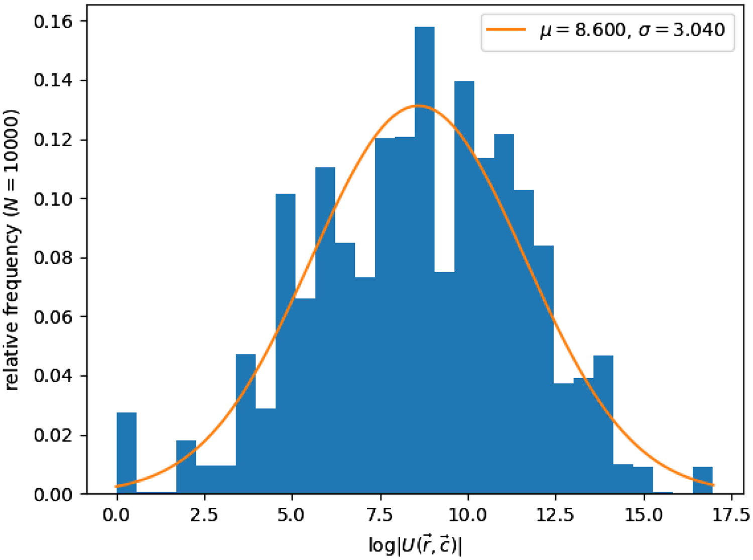
Figure 7. A histogram of the logarithm $\log |\mathfrak U(\vec r,\vec s)|$
of the number of binary matrices with the same row and column sums as a Battleship fleet, generated using a population of 10,000 randomly generated fleets. The minimum, mean and maximum number of matrices were 1,
$\log |\mathfrak U(\vec r,\vec s)|$
of the number of binary matrices with the same row and column sums as a Battleship fleet, generated using a population of 10,000 randomly generated fleets. The minimum, mean and maximum number of matrices were 1, $5431.66$
and 23,950,440, respectively.
$5431.66$
and 23,950,440, respectively.
However, calculating the density of Battleship fleets requires explicit computation of all the elements of $\mathfrak U(\vec r,\vec c)$
, which is computationally intensive. Even so, in a sample of 30 randomly generated Battleship fleets, the number of fleet positions in
$\mathfrak U(\vec r,\vec c)$
, which is computationally intensive. Even so, in a sample of 30 randomly generated Battleship fleets, the number of fleet positions in $\mathfrak U(\vec r,\vec c)$
had mean 3, median 2, min 1 and max 9. This indicates that the density of Battleship fleets is typically very small.
$\mathfrak U(\vec r,\vec c)$
had mean 3, median 2, min 1 and max 9. This indicates that the density of Battleship fleets is typically very small.
4. Reconstructing fleet positions
In this section, we describe our method of reconstructing fleet positions from knowledge of the row and column sums. Our strategy is to reformulate the problem as a QUBO problem of finding the $10\times 10$
binary matrices with the correct row or column sums whose values are near the minimum of the square of the two-dimensional discrete Laplacian.
$10\times 10$
binary matrices with the correct row or column sums whose values are near the minimum of the square of the two-dimensional discrete Laplacian.
4.1. Converting to QUBO
Let Q be an $n\times n$
matrix, L an
$n\times n$
matrix, L an $m\times n$
matrix and
$m\times n$
matrix and $\vec b$
length m vector satisfying
$\vec b$
length m vector satisfying $L\vec x = \vec b$
for some
$L\vec x = \vec b$
for some $\vec x\in\{0,1\}^n$
. Consider the linearly constrained binary optimisation problem of minimising
$\vec x\in\{0,1\}^n$
. Consider the linearly constrained binary optimisation problem of minimising $\vec x^TQ\vec x$
subject to the constraint that
$\vec x^TQ\vec x$
subject to the constraint that $L\vec x = \vec b$
. It turns out that such a constrained problem can be converted into a QUBO problem in a standard way.
$L\vec x = \vec b$
. It turns out that such a constrained problem can be converted into a QUBO problem in a standard way.
Theorem 4.1. Let Q and L be as above and define
 \begin{equation*}Q_{\text{lin}} = L^TL - 2\text{diag}(L^T\vec b).\end{equation*}
For $\epsilon$
small enough, solutions of the QUBO problem
$\epsilon$
small enough, solutions of the QUBO problem
 \begin{equation}\text{minimize}\ \vec x^T(Q_{\text{lin}} + \epsilon Q)\vec x,\quad \vec x\in\{0,1\}^n\end{equation}
will also be solutions of the optimisation problem with a linear constraint
 \begin{equation}\text{minimize}\ \vec x^TQ\vec x,\quad \vec x\in \{0,1\}^n,\ L\vec x= \vec b\end{equation}
Proof. First note that
 \begin{equation*}\vec x^TL^TL\vec x - 2\vec x^TL^T\vec b + \vec b^T\vec b = (L\vec x-b)^T(L\vec x - \vec b) \geq 0\end{equation*}
with equality if and only if $L\vec x = \vec b$
. Since
$L\vec x = \vec b$
. Since $\vec x$
is binary,
$\vec x$
is binary, $\vec x^T\vec L^T\vec b = \vec x^T\text{diag}(\vec L^T\vec b)\vec x$
. Therefore, we can see
$\vec x^T\vec L^T\vec b = \vec x^T\text{diag}(\vec L^T\vec b)\vec x$
. Therefore, we can see
 \begin{equation*}\vec x^TQ_{\text{lin}}\vec x + \vec b^T\vec b\geq 0\end{equation*}
with equality if and only if $L\vec x = \vec b$
. In particular, solutions of the QUBO problem
$L\vec x = \vec b$
. In particular, solutions of the QUBO problem
 \begin{equation*}\text{minimize}\ \vec x^TQ_{\text{lin}}\vec x,\quad \vec x\in\{0,1\}^n.\end{equation*}
are precisely the binary solutions of the linear system of equations $L\vec x = \vec b$
. Note that viewed as an optimisation problem, the constant term
$L\vec x = \vec b$
. Note that viewed as an optimisation problem, the constant term $\vec b^T\vec b$
may be ignored.
$\vec b^T\vec b$
may be ignored.
Now consider the partition of the space of binary vectors consisting of the set $U = \{\vec x\in \{0,1\}^n \;:\; L\vec x = \vec b\}$
and its complement
$U = \{\vec x\in \{0,1\}^n \;:\; L\vec x = \vec b\}$
and its complement $U^c = \{\vec x\in \{0,1\}^n \;:\; L\vec x \neq \vec b\}$
. Let R be the
$U^c = \{\vec x\in \{0,1\}^n \;:\; L\vec x \neq \vec b\}$
. Let R be the $L^2$
-norm of Q and take
$L^2$
-norm of Q and take $\epsilon < r/(2nR)$
for
$\epsilon < r/(2nR)$
for $r = \min_{\vec x\in U^{\prime}} (x^TQ_{\text{lin}}\vec x + \vec b^T\vec b)$
. Then for any
$r = \min_{\vec x\in U^{\prime}} (x^TQ_{\text{lin}}\vec x + \vec b^T\vec b)$
. Then for any $\vec x \in \{0,1\}^n$
, we have
$\vec x \in \{0,1\}^n$
, we have $\epsilon |\vec x^TQ\vec x| < r/2$
. Therefore,
$\epsilon |\vec x^TQ\vec x| < r/2$
. Therefore,
 \begin{equation*}\min_{\vec x\in U} \vec x^T(Q_{\text{lin}} + \epsilon Q)\vec x + \vec b^T\vec b = \min_{\vec x\in U} \epsilon\vec x^TQ\vec x < r/2\end{equation*}
while by the triangle inequality
 \begin{equation*}\min_{\vec x\in U^c} \vec x^T(Q_{\text{lin}} + \epsilon Q)\vec x + \vec b^T\vec b \geq \min_{\vec x\in U^c} r - \epsilon |\vec x^TQ\vec x| > r/2.\end{equation*}
In particular, the solution of the QUBO problem
 \begin{equation*}\text{minimize}\ \vec x^T(Q_{\text{lin}} + \epsilon Q)\vec x,\quad \vec x\in\{0,1\}^n\end{equation*}
will belong to U. This completes the proof.
Remark 4.2. The value $\epsilon$
in the theorem above works as a parameter which must be adjusted to be small enough that solutions of the QUBO problem satisfy the linear constraint
$\epsilon$
in the theorem above works as a parameter which must be adjusted to be small enough that solutions of the QUBO problem satisfy the linear constraint $L\vec x = \vec b$
, but large enough so that the
$L\vec x = \vec b$
, but large enough so that the $\epsilon Q$
term is sufficiently significant. The above proof suggests taking
$\epsilon Q$
term is sufficiently significant. The above proof suggests taking $\epsilon$
to be on the order of
$\epsilon$
to be on the order of $r/(2nR)$
, which can be very small. However, as one helpful referee pointed out, when Q is positive semidefinite the proof can be adjusted to take
$r/(2nR)$
, which can be very small. However, as one helpful referee pointed out, when Q is positive semidefinite the proof can be adjusted to take $\epsilon < r/\min_{x\in U}\vec x^TQ\vec x$
, which can be magnitudes larger. In practice, a reasonable value of
$\epsilon < r/\min_{x\in U}\vec x^TQ\vec x$
, which can be magnitudes larger. In practice, a reasonable value of $\epsilon$
can be determined from direct numerical experimentation.
$\epsilon$
can be determined from direct numerical experimentation.
Thus, to solve the problem of finding binary matrices with certain row and column sums which minimise the Laplacian, we can convert the associated linear system to a QUBO problem with matrix $Q_{\text{lin}}$
, construct a matrix
$Q_{\text{lin}}$
, construct a matrix $Q_{\text{lap}}$
encoding the Laplacian and solve the QUBO problem for the matrix
$Q_{\text{lap}}$
encoding the Laplacian and solve the QUBO problem for the matrix
 \begin{equation*}Q = Q_{\text{lin}}+\epsilon Q_{\text{lap}}\end{equation*}
for sufficiently small $\epsilon$
. We discuss this in detail in the next subsection.
$\epsilon$
. We discuss this in detail in the next subsection.
4.2. Laplacian-minimising solutions
To calculate the Laplacian-minimising $10\times 10$
binary matrices A with prescribed row and column sums, we start by expressing A as a binary vector
$10\times 10$
binary matrices A with prescribed row and column sums, we start by expressing A as a binary vector $\vec x$
of length 100 whose entries are
$\vec x$
of length 100 whose entries are $x_{10(j-1)+k}=A_{jk}$
with
$x_{10(j-1)+k}=A_{jk}$
with $1\leq j,k\leq 10$
. Taking the row and column sums of A is then equivalent to multiplying
$1\leq j,k\leq 10$
. Taking the row and column sums of A is then equivalent to multiplying $\vec x$
by a
$\vec x$
by a $20\times100$
matrix L whose entries are
$20\times100$
matrix L whose entries are
 \begin{equation*}L_{m,10(j-1)+k} = \left\lbrace\begin{array}{c@{\quad}c}1, & 1\leq m\leq 10\ \text{and}\ m = k\\[4pt]1, & 11\leq m\leq 20\ \text{and}\ j= m-10\\[4pt]0, & \text{otherwise}\end{array}\right.\!\!,\quad 1\leq j,k\leq 10\end{equation*}
In particular, if $\vec r$
and
$\vec r$
and $\vec c$
are column vectors whose entries are the row and column sums of A (in order from top to bottom or left to right) then
$\vec c$
are column vectors whose entries are the row and column sums of A (in order from top to bottom or left to right) then $L\vec x = \binom{\vec r}{\vec c}$
.
$L\vec x = \binom{\vec r}{\vec c}$
.
The discrete Laplacian of a matrix A is a new matrix $\Delta A$
whose size is the same as A and whose entries are
$\Delta A$
whose size is the same as A and whose entries are
 \begin{equation*}(\Delta A)_{j,k}=4A_{j,k}-A_{j-1,k}-A_{j+1,k}-A_{j,k-1}-A_{j,k+1},\end{equation*}
where entries $A_{m,n}$
outside the bounds of
$A_{m,n}$
outside the bounds of $1,\dots, 10$
are taken to be zero. This corresponds to the multiplication of
$1,\dots, 10$
are taken to be zero. This corresponds to the multiplication of $\vec x$
by a
$\vec x$
by a $100\times 100$
matrix, which as an abuse of notation we also denote by
$100\times 100$
matrix, which as an abuse of notation we also denote by $\Delta$
:
$\Delta$
:
 \begin{equation*}\Delta_{10(s-1)+t,10(j-1)+k} = \left\lbrace\begin{array}{c@{\quad}c}4, & s=j\ \text{and}\ t=k\\[4pt]-1, & s=j\ \text{and}\ |t-k|=1\\[4pt]-1, & t=k\ \text{and}\ |s-j|=1\\[4pt]0, & \text{otherwise}.\end{array}\right.,\quad 1\leq j,k\leq 10.\end{equation*}
In this form, the sum of the squares of the Laplacian of a matrix A is equal to the product $\vec x^T(\Delta^T\Delta) \vec x$
where
$\vec x^T(\Delta^T\Delta) \vec x$
where $\vec x$
is the vector version of A.
$\vec x$
is the vector version of A.
Thus, the search for binary matrices A with prescribed row sums and column sums given by $\vec r = [r_1\ \dots\ r_{10}]^T$
and
$\vec r = [r_1\ \dots\ r_{10}]^T$
and $\vec c=[c_1\ \dots\ c_{10}]$
, respectively, which minimise the square-sum of the discrete Laplacian, is equivalent to the QUBO problem
$\vec c=[c_1\ \dots\ c_{10}]$
, respectively, which minimise the square-sum of the discrete Laplacian, is equivalent to the QUBO problem
 \begin{equation}\text{minimize}\quad \vec x^T(Q_{\text{lin}}+\epsilon Q_{\text{lap}})\vec x,\quad x\in \{0,1\}^{100},\end{equation}
where here $Q_{\text{lap}} = \Delta^T\Delta$
and
$Q_{\text{lap}} = \Delta^T\Delta$
and
 \begin{equation*}Q_{\text{lin}} = L^TL-2\text{diag}([r_1\ \dots\ r_{10}\ c_1\dots\ c_{10}]L).\end{equation*}
In practice, the value of $\epsilon$
is a parameter that we can tune to potentially improve performance. The results of our numerical experiments below were obtained using a value of
$\epsilon$
is a parameter that we can tune to potentially improve performance. The results of our numerical experiments below were obtained using a value of $\epsilon = 0.005$
.
$\epsilon = 0.005$
.
4.3. Numerical methods
To investigate the practicality of our method of reconstructing fleet positions via solving QUBO problems, we used two common metaheuristic solving methods: tabu and simulated annealing. Starting with a randomly generated Battleship fleet, we construct the QUBO problem associated with the given row and column sums, as described in the previous section. Then we try to reconstruct a fleet with the same row and column sums using one of these QUBO solvers. Note that we are not interested in whether or not we recover the specific Battleship fleet we started with, since we anticipate generalised Ryser interchanges to allow us to quickly move from a recovered fleet position to the original one. This has been the situation in every case we have observed, though we have not completed a detailed investigation.
The tabu search method approximates a solution of the QUBO problem of minimising the quadratic potential energy $E(\vec x) = \vec x^TQ\vec x$
by iteratively updating an approximate solution and then moving to the adjacent vector with lowest potential energy, excluding a certain list of tabu or forbidden states. After many iterations, the presence of a large set of forbidden states may cause iterations to increase rather than decrease the potential energy, allowing the algorithm to escape local minima in the potential energy and more successfully obtain global minima. For details and applications, see [Reference Glover11, Reference Glover12].
$E(\vec x) = \vec x^TQ\vec x$
by iteratively updating an approximate solution and then moving to the adjacent vector with lowest potential energy, excluding a certain list of tabu or forbidden states. After many iterations, the presence of a large set of forbidden states may cause iterations to increase rather than decrease the potential energy, allowing the algorithm to escape local minima in the potential energy and more successfully obtain global minima. For details and applications, see [Reference Glover11, Reference Glover12].

Figure 8. Performance of tabu search versus number of iterations on reconstructing randomly generated fleets from their row and column sums, based on an average of 1000 randomly chosen Battleship fleets. For $\geq 200$
iterations, upwards of 92% of randomly generated fleets are able to be reconstructed via this search method. The axis on the left represents the number of reads taken for the simulated annealing algorithm. The right axis shows the number of restarts taken for tabu search algorithm.
$\geq 200$
iterations, upwards of 92% of randomly generated fleets are able to be reconstructed via this search method. The axis on the left represents the number of reads taken for the simulated annealing algorithm. The right axis shows the number of restarts taken for tabu search algorithm.
A simulated annealer works by starting with an initial binary vector $\vec x$
and then jumping to a random neighbouring vector which is either of lower energy or potentially of higher energy but with a probability which decreases based on the iteration. For an introductory account, see [Reference Aarts and Van Laarhoven1].
$\vec x$
and then jumping to a random neighbouring vector which is either of lower energy or potentially of higher energy but with a probability which decreases based on the iteration. For an introductory account, see [Reference Aarts and Van Laarhoven1].
We used simulated annealing as a substitute for an actual quantum annealer, in order to predict the feasibility of solving our QUBO problem a quantum computer. We expect that QUBO problems which can be solved by simulated annealing should also be approachable by quantum annealing. Likewise, evidence suggests that “hard” QUBO problems, ones where traditional algorithms fail to identify optimal solutions, exhibit the same pitfalls on current quantum architectures [Reference Vert, Sirdey and Louise27]. Of course, this ignores certain other potential barriers to implementation, such as limitations imposed by the hardware topology. As the scale of quantum computers increases, it is hoped that quantum phenomena will allow quantum annealers to outperform the classical case, even on difficult problems [Reference Vert, Sirdey and Louise27].
For our work, we use the tabu search algorithm implemented by the QBSolv library in Python [Reference Booth, Reinhardt and Roy6], which is based on a multistart tabu search method described in [Reference Palubeckis22] using randomly generated initial states. The main parameter we adjust in this algorithm is the number of times we restart the search algorithm using a different randomly generated initial state. The algorithm then returns a list of the minimum energy states found after each restart, which is typically much smaller than the number of restarts do to the presence of duplicates. We also used the simulated annealing python library dwave-neal available from D-Wave Systems [8], where the main adjustment parameter is the number of reads, with each read representing a separate run of the simulated annealing algorithm from a different starting position. We consider a reconstruction to be successful if one of the fleets returned has a Battleship fleet realisation.
To get an idea of the viability of both algorithms, we observed the fraction of successful reconstructions starting with a sample of 1000 randomly generated Battleship fleets. As shown in Figure 8, we are able to obtain a Battleship fleet with the desired row and column sums over 92% of the time for randomly generated Battleship fleets, as long as we use $ 1000$
algorithm restarts in the tabu search algorithm. The behaviour of the simulated annealer is similarly successful in solving a similar number of Battleship puzzle problems, as we use
$ 1000$
algorithm restarts in the tabu search algorithm. The behaviour of the simulated annealer is similarly successful in solving a similar number of Battleship puzzle problems, as we use $ 10,000$
algorithm reads. Note that both experiments are shown on the same plot to facilitate their comparison. To accommodate this, the left axis denotes the number of reads taken for the simulated annealing algorithm. The right axis denotes the number of restarts taken for the tabu search algorithm.
$ 10,000$
algorithm reads. Note that both experiments are shown on the same plot to facilitate their comparison. To accommodate this, the left axis denotes the number of reads taken for the simulated annealing algorithm. The right axis denotes the number of restarts taken for the tabu search algorithm.
The fact that both algorithms perform well suggests that the majority of Battleship puzzle problems lead to QUBO problems which are solvable by standard methods. We likewise anticipate that a true quantum computer would successfully solve most cases.
Cases that fail tend to demonstrate many alternative configurations of the binary matrix with lower energy than actual solutions. In the future, it would be interesting to characterise the Battleship fleets which lead to hard QUBO problems that the algorithms fail to solve.
5. Reconstructing other binary matrices
The method proposed for reconstructing certain kinds of binary matrices from their tomographic data naturally lends itself to more types of matrices than Battleship fleets. In particular, it is natural to expect that a wide variety of binary matrices, such as binary images, will naturally have smooth edges and thus smaller Laplacians than other objects with the same tomographic data.
In general, as the size of binary matrices increases, the size of $\mathfrak U(\vec r,\vec c)$
characteristically grows at least factorially. For example, in the case that the row and column sums are all 1, the set
$\mathfrak U(\vec r,\vec c)$
characteristically grows at least factorially. For example, in the case that the row and column sums are all 1, the set $\mathfrak U(\vec r,\vec c)$
of
$\mathfrak U(\vec r,\vec c)$
of $n\times n$
binary matrices with this tomographic data is exactly the set of permutation matrices and has size
$n\times n$
binary matrices with this tomographic data is exactly the set of permutation matrices and has size $n!$
. For large n, the prospect of searching such a space for the matrices for a particular matrix is daunting. This makes the potential quantum speedup of the QUBO formulation on future quantum hardware particularly appealing.
$n!$
. For large n, the prospect of searching such a space for the matrices for a particular matrix is daunting. This makes the potential quantum speedup of the QUBO formulation on future quantum hardware particularly appealing.
5.1. Two convex bodies
As a basic test case, we consider a $20\times 20$
matrix whose nonzero entries consist of two convex bodies, as shown in Figure 9 below.
$20\times 20$
matrix whose nonzero entries consist of two convex bodies, as shown in Figure 9 below.

Figure 9. A $20\times 20$
binary matrix consisting of two convex bodies. The Laplacian norm squared-minimising QUBO problem formulated here successfully recovers this image exactly from its binary tomographic data.
$20\times 20$
binary matrix consisting of two convex bodies. The Laplacian norm squared-minimising QUBO problem formulated here successfully recovers this image exactly from its binary tomographic data.

Figure 10. Several $9\times 9$
matrices with the same tomographic data. The value of the norm squared of the Laplacian is listed below each figure. The original image of the heart has a larger Laplacian value than the others.
$9\times 9$
matrices with the same tomographic data. The value of the norm squared of the Laplacian is listed below each figure. The original image of the heart has a larger Laplacian value than the others.
In this instance, the set $\mathfrak U(\vec r,\vec c)$
of binary matrices with the same row and column sums as the matrix in Figure 9 is very large and prohibitively computationally intensive to compute. Despite this, the number of matrices in
$\mathfrak U(\vec r,\vec c)$
of binary matrices with the same row and column sums as the matrix in Figure 9 is very large and prohibitively computationally intensive to compute. Despite this, the number of matrices in $\mathfrak U(\vec r,\vec c)$
can be computed using the recursive algorithm proposed in [Reference Miller and Harrison21] and is computed to be 681981424292938974077440 (approx.
$\mathfrak U(\vec r,\vec c)$
can be computed using the recursive algorithm proposed in [Reference Miller and Harrison21] and is computed to be 681981424292938974077440 (approx. $6.8\times 10^{24}$
). Based on a sample of
$6.8\times 10^{24}$
). Based on a sample of $2\times 10^5$
of these matrices, the original figure has minimal norm-squared Laplacian. This explains the success of the QUBO problem formulation in recovering the original image.
$2\times 10^5$
of these matrices, the original figure has minimal norm-squared Laplacian. This explains the success of the QUBO problem formulation in recovering the original image.
5.2. Heartier QUBO formulations
For more complicated shapes, simply minimising the norm squared of the Laplacian may be insufficient to recover the original image from its tomographic data. For example, the shape of a $9\times 9$
binary heart is not directly found by our methods due to the presence of tomographically equivalent matrices with smaller Laplacians, as shown in Figure 10. Minimising the gradient squared runs into this same issue.
$9\times 9$
binary heart is not directly found by our methods due to the presence of tomographically equivalent matrices with smaller Laplacians, as shown in Figure 10. Minimising the gradient squared runs into this same issue.
To fix this, we can again take our inspiration from Battleship and imagine that we have fired a number of shots so that we know definitively the values of entries at certain locations. Using the same process as we did above to impose the linear constraint that the matrix satisfy certain tomographic data, we can impose the additional linear constraints that its value is equal to a particular number in some number of places. By imposing just a few such additional constraints at strategically chosen locations, such as at the three tips of the heart, we are able to recover our original heart shape.
6. Summary
In this paper, we considered the Battleship puzzle problem from the point of view of discrete tomography and quantum computing. We demonstrated the existence of different battleship fleets with the same discrete tomographic data and showed how to create new fleets with identical tomographic data from old ones via generalised Ryser interchanges. We demonstrated empirically that Battleship fleets tend to have lower values for the norm squared of their Laplacians, compared to other discrete binary matrices with the same row and column sums. Using this, we constructed a QUBO-based algorithm for reconstructing Battleship fleets from their row and column sum data. Lastly, we demonstrated the success of this algorithm using both tabu-based and simulated annealing search algorithms. The latter provides evidence that similar sort of Laplacian-minimising QUBO problems could be successfully solved on a quantum annealer.
Acknowledgements
The authors would like to thank the referees for their insight and thoughtful comments which have been a great help in improving the present manuscript.
Conflict of interests
The authors declare there is no conflict of interest.


 Open access