


1 Introduction
We investigate the existence and uniqueness of solutions to the Helmholtz equation
 \begin{equation} -\nabla\cdot (a\nabla u) - \omega^2 u = f\end{equation}
in an infinite wave guide $\Omega := \mathbb{R} \times S$
. The cross-section S is given by a bounded Lipschitz domain
$\Omega := \mathbb{R} \times S$
. The cross-section S is given by a bounded Lipschitz domain $S\subset \mathbb{R}^{d-1}$
, the right hand side
$S\subset \mathbb{R}^{d-1}$
, the right hand side $f\in H^{-1}(\Omega)$
has compact support; below, the frequency
$f\in H^{-1}(\Omega)$
has compact support; below, the frequency $\omega>0$
is assumed to be non-singular. The differential operator
$\omega>0$
is assumed to be non-singular. The differential operator $A u := -\nabla\cdot (a\nabla u)$
is given by coefficients
$A u := -\nabla\cdot (a\nabla u)$
is given by coefficients $a: \Omega\to \mathbb{R}^{d\times d}$
of class
$a: \Omega\to \mathbb{R}^{d\times d}$
of class $L^\infty(\Omega)$
with a(x) symmetric and positive for every x, satisfying
$L^\infty(\Omega)$
with a(x) symmetric and positive for every x, satisfying $\lambda |\xi|^2 \le \xi\cdot a(x)\xi \le \Lambda |\xi|^2$
for some
$\lambda |\xi|^2 \le \xi\cdot a(x)\xi \le \Lambda |\xi|^2$
for some $0 < \lambda < \Lambda < \infty$
and all
$0 < \lambda < \Lambda < \infty$
and all $\xi\in \mathbb{R}^d$
,
$\xi\in \mathbb{R}^d$
, $x\in \Omega$
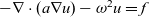
. We treat two settings: Periodic coefficients, that is, coefficients a that satisfy
$x\in \Omega$
. We treat two settings: Periodic coefficients, that is, coefficients a that satisfy $a(x + e_1) = a(x)$
for every
$a(x + e_1) = a(x)$
for every $x\in \Omega$
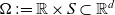
, see Figure 1. The other setting is that of coefficients a that are periodic at the far left and at the far right and arbitrary in a central region: There exists
$x\in \Omega$
, see Figure 1. The other setting is that of coefficients a that are periodic at the far left and at the far right and arbitrary in a central region: There exists $R_0>0$
such that
$R_0>0$
such that $a(x + e_1) = a(x)$
for every
$a(x + e_1) = a(x)$
for every $x\in \Omega$
with
$x\in \Omega$
with $|x_1|>R_0$
, see Figure 2. We impose a Neumann condition on
$|x_1|>R_0$
, see Figure 2. We impose a Neumann condition on $\partial\Omega$
; Dirichlet conditions can be treated in the same way.
$\partial\Omega$
; Dirichlet conditions can be treated in the same way.
Figure 1. The wave guide geometry in two dimensions. The coefficient a is indicated by different levels of grey. It is 1-periodic in $x_1$
-direction.
$x_1$
-direction.
We say that a function $u \in H^1_\mathrm{loc}(\Omega)$
solves the radiation problem if the following three conditions are met:
$u \in H^1_\mathrm{loc}(\Omega)$
solves the radiation problem if the following three conditions are met:
-
(i) u solves (1.1) in $\Omega$
in the weak sense.
$\Omega$
in the weak sense. -
(ii)
$\sup_{r\in \mathbb{Z}} \| u \|_{L^2((r,r+1)\times S)} < \infty$
. -
(iii) the radiation condition of Definition 2.4 is satisfied.


Regarding the radiation condition, we note that Definition 2.4 is equivalent to a more standard condition, see Lemma 3.2. One of our main results is the following existence and uniqueness statement.
Theorem 1.1 (Existence and uniqueness result for periodic media). Let the data $\Omega$
, f,
$\Omega$
, f, $\omega$
, and a be as above, the coefficients 1–periodic in
$\omega$
, and a be as above, the coefficients 1–periodic in $x_1$
, that is:
$x_1$
, that is: $a(x + e_1) = a(x)$
for every
$a(x + e_1) = a(x)$
for every $x\in \Omega$
. Let
$x\in \Omega$
. Let $\omega$
be non-singular in the sense of Definition 2.3 below. Then, there exists one and only one solution u to the radiation problem (i)–(iii).
$\omega$
be non-singular in the sense of Definition 2.3 below. Then, there exists one and only one solution u to the radiation problem (i)–(iii).
The statement of Theorem 1.1 is not new, but contained, for example, in [Reference Fliss and Joly9] (Theorem 1.2 below is the new result of this article). The decisive difference between existing literature and the paper at hand regards the methods of proof. The proof in [Reference Fliss and Joly9] uses operator theory (just as the proofs of similar results in [Reference Hoang10 Reference Kirsch and Lechleiter13, Reference Radosz20]): One constructs families of operators in subsets of the complex plane, sketches specific curves in the complex plane and evaluates corresponding line integrals of operators. The constructions provide bounded families of operators and thus, as a result, an inverse to the Helmholtz operator. The proofs rely on analyticity properties and exploit Kato’s perturbation theory for operators.
By contrast, our proof uses only energy methods and is self-contained. Using only energy methods means here that (a) we only use $L^2$
-based function spaces, (b) the existence result is obtained from a priori estimates, (c) the a priori estimates are obtained with the help of appropriately chosen test functions for the equations. Energy conservation of the physical system is reflected by the mathematical fact that the energy flux is independent of the position, see Remark 2.2. The flux equality in the form of Lemmas 2.1 and A.1 is the central tool in the proofs of the main results, Theorems 1.1 and 1.2. This article is self-contained in the sense that the proofs of the two main theorems use only standard theory of partial differential equations. The further analysis of the non-singularity assumption for the frequency
$L^2$
-based function spaces, (b) the existence result is obtained from a priori estimates, (c) the a priori estimates are obtained with the help of appropriately chosen test functions for the equations. Energy conservation of the physical system is reflected by the mathematical fact that the energy flux is independent of the position, see Remark 2.2. The flux equality in the form of Lemmas 2.1 and A.1 is the central tool in the proofs of the main results, Theorems 1.1 and 1.2. This article is self-contained in the sense that the proofs of the two main theorems use only standard theory of partial differential equations. The further analysis of the non-singularity assumption for the frequency $\omega$
is not the aim of this contribution.
$\omega$
is not the aim of this contribution.
Our results have the character of a Fredholm alternative. The assumption that the frequency $\omega$
is non-singular implies that the homogeneous problem has only the trivial solution. From this uniqueness property, we obtain the existence result. In order to obtain the existence, we introduce an approximate problem which is easy to solve. If the approximate solutions are bounded, then any limit is the desired solution to the original problem. If the approximate solutions are unbounded, we normalise them and obtain, in the limit, a nontrivial solution to the homogeneous problem – in contradiction to the uniqueness property.
$\omega$
is non-singular implies that the homogeneous problem has only the trivial solution. From this uniqueness property, we obtain the existence result. In order to obtain the existence, we introduce an approximate problem which is easy to solve. If the approximate solutions are bounded, then any limit is the desired solution to the original problem. If the approximate solutions are unbounded, we normalise them and obtain, in the limit, a nontrivial solution to the homogeneous problem – in contradiction to the uniqueness property.
From the above description of the proof, it is clear that the approach is very direct. The two difficulties are (1) the construction of a useful approximate problem and (2) the verification of the radiation condition for limits. Our choice is inspired by constructions of [Reference Dohnal and Schweizer5] and [Reference Lamacz and Schweizer18]. We work with truncated domains and radiation boxes to formulate boundary conditions. We demand that approximate solutions look like outgoing waves in the radiation boxes. The proofs rely on the flux equality for solutions: In every cross-section of the wave guide, the solution has the same energy flux.
Figure 2. A non-periodic coefficient a as in Theorem 1.2. The coefficient is periodic as $x_1\to \infty$
and as
$x_1\to \infty$
and as $x_1\to -\infty$
. The medium satisfies
$x_1\to -\infty$
. The medium satisfies $a(x + e_1) = a(x)$
for every
$a(x + e_1) = a(x)$
for every $x\in \Omega$
with
$x\in \Omega$
with $|x_1|>R_0$
for
$|x_1|>R_0$
for $R_0 = 5$
. The two periodic media (far left and far right) can be different.
$R_0 = 5$
. The two periodic media (far left and far right) can be different.
Our methods are very flexible and provide also new results. The next theorem treats a medium that is arbitrary on a compact subdomain and periodic outside of that subdomain. Our assumption on the medium can also be formulated as follows: There are two periodic fields $a^\mathrm{left}, a^\mathrm{right}: \Omega\to \mathbb{R}^{d\times d}$
,
$a^\mathrm{left}, a^\mathrm{right}: \Omega\to \mathbb{R}^{d\times d}$
, $a^\mathrm{left}(x + e_1) = a^\mathrm{left}(x)$
and
$a^\mathrm{left}(x + e_1) = a^\mathrm{left}(x)$
and $a^\mathrm{right}(x + e_1) = a^\mathrm{right}(x)$
for every
$a^\mathrm{right}(x + e_1) = a^\mathrm{right}(x)$
for every $x\in \Omega$
. The coefficient a is of class
$x\in \Omega$
. The coefficient a is of class $L^\infty(\Omega)$
, and it is pointwise symmetric and positive and has the ellipticity bounds
$L^\infty(\Omega)$
, and it is pointwise symmetric and positive and has the ellipticity bounds $\Lambda>\lambda>0$
. It satisfies, for some
$\Lambda>\lambda>0$
. It satisfies, for some $R_0 > 0$
:
$R_0 > 0$
:
 \begin{align*} a(x) &= a^\mathrm{left}(x) \qquad \text{if } x_1 < - R_0\,,\\[3pt] a(x) &= a^\mathrm{right}(x) \qquad \text{if } x_1 > R_0\,.\end{align*}
For such a medium, even if $\omega$
is non-singular for
$\omega$
is non-singular for $a^\mathrm{left}$
and
$a^\mathrm{left}$
and $a^\mathrm{right}$
, the number
$a^\mathrm{right}$
, the number $\omega^2$
can be an eigenvalue of the elliptic operator A. We therefore have to assume the uniqueness property for the homogeneous problem.
$\omega^2$
can be an eigenvalue of the elliptic operator A. We therefore have to assume the uniqueness property for the homogeneous problem.
Theorem 1.2 (Media that are periodic at infinity). Let the wave guide $\Omega= \mathbb{R} \times S$
be as above. Let
$\Omega= \mathbb{R} \times S$
be as above. Let $a: \Omega\to \mathbb{R}^{d\times d}$
be essentially bounded, symmetric and positive as above. We assume that, for some
$a: \Omega\to \mathbb{R}^{d\times d}$
be essentially bounded, symmetric and positive as above. We assume that, for some $R_0>0$
,
$R_0>0$
,
 \begin{equation*} a(x + e_1) = a(x)\quad \text{ for every $x\in \Omega$ with } |x_1| > R_0 \,, \end{equation*}
which implies that a coincides with $a^\mathrm{left}$
and
$a^\mathrm{left}$
and $a^\mathrm{right}$
outside a compact region for some periodic coefficients
$a^\mathrm{right}$
outside a compact region for some periodic coefficients $a^\mathrm{left}$
and
$a^\mathrm{left}$
and $a^\mathrm{right}$
. Let
$a^\mathrm{right}$
. Let $\omega>0$
be a non-singular frequency in the sense of Definition 2.3 below for the two periodic media given by
$\omega>0$
be a non-singular frequency in the sense of Definition 2.3 below for the two periodic media given by $a^\mathrm{left}$
and
$a^\mathrm{left}$
and $a^\mathrm{right}$
. If the radiation problem (i)–(iii) with
$a^\mathrm{right}$
. If the radiation problem (i)–(iii) with $f=0$
possesses only the trivial solution, then the radiation problem (i)–(iii) has a unique solution u for arbitrary
$f=0$
possesses only the trivial solution, then the radiation problem (i)–(iii) has a unique solution u for arbitrary $f\in H^{-1}(\Omega)$
with compact support.
$f\in H^{-1}(\Omega)$
with compact support.
We emphasise that the medium in the above theorem is not necessarily a compact perturbation of a periodic medium. Our proof works also when a compact perturbation of the underlying geometry $\Omega = \mathbb{R} \times S$
is considered, for example, when the channel is thicker in a central region. Moreover, the unbounded half-channels could have also different cross-sections or they could lead in different directions.
$\Omega = \mathbb{R} \times S$
is considered, for example, when the channel is thicker in a central region. Moreover, the unbounded half-channels could have also different cross-sections or they could lead in different directions.
Regarding literature, we mention [Reference Kress15] for classical methods. We note that some of the references below treat the problem on the whole space $\mathbb{R}^d$
; some results on that problem can be interpreted as statements on the wave guide problem with periodicity boundary condition in the bounded direction. In this sense, the line defect analysis of [Reference Hoang and Radosz11] provides a uniqueness result for a local perturbation of a periodic medium. In general, uniqueness does not hold in the situation of Theorem 1.2, see [Reference Ammari and Santosa1, Reference Evans, Linton and Ursell6, Reference Figotin and Klein7]. For another form of a radiation condition, we mention [Reference Kirsch and Lechleiter13]. The work [Reference Coatléven4] treats a similar problem and makes a connection to a Lippmann-Schwinger equation; uniqueness is obtained there from a positive absorption parameter. An interface with a metamaterial is considered in [Reference Bonnet-Ben Dhia, Chesnel and Claeys2].
$\mathbb{R}^d$
; some results on that problem can be interpreted as statements on the wave guide problem with periodicity boundary condition in the bounded direction. In this sense, the line defect analysis of [Reference Hoang and Radosz11] provides a uniqueness result for a local perturbation of a periodic medium. In general, uniqueness does not hold in the situation of Theorem 1.2, see [Reference Ammari and Santosa1, Reference Evans, Linton and Ursell6, Reference Figotin and Klein7]. For another form of a radiation condition, we mention [Reference Kirsch and Lechleiter13]. The work [Reference Coatléven4] treats a similar problem and makes a connection to a Lippmann-Schwinger equation; uniqueness is obtained there from a positive absorption parameter. An interface with a metamaterial is considered in [Reference Bonnet-Ben Dhia, Chesnel and Claeys2].
Regarding the spectral properties of the Helmholtz operator, we mention [Reference Nazarov and Plamenevsky19]; Theorem 3.2 in Chapter 5 of that reference provides in certain settings that all frequencies $\omega>0$
are non-singular in the sense of Definition 2.3. The existence of Floquet modes is shown in [Reference Hohage and Soussi12].
$\omega>0$
are non-singular in the sense of Definition 2.3. The existence of Floquet modes is shown in [Reference Hohage and Soussi12].
We mention that the Fredholm alternative for a limiting absorption principle was also exploited in [Reference Schweizer and Urban22] in order to improve the existence statement of [Reference Dohnal and Schweizer5] with a vanishing absorption principle. Similar methods are also used in [Reference Bonnet-Ben Dhia, Chesnel and Claeys2]. The analysis of guided modes in a wave guide with purely harmonic dependence in the unbounded direction was treated in [Reference Bonnet-Ben Dhia and Joly3]. In the work [Reference Fliss8], the solution to half-space problems is used for the computation of guided modes, which is further exploited in [Reference Klindworth, Schmidt and Fliss14].
It is worth noting at this point that our results have the drawback that they do not include a limiting absorption principle for the unbounded domain. This fact is related to the method of proof since we construct approximate solutions with truncated problems and not with a small absorption parameter.
2 Preliminaries
In this section, we discuss various properties of the system and specify the setting for our results. We start with the conservation of fluxes. This is a fundamental property of the Helmholtz equation, and our existence result is built on it. We recall the concept of propagating modes and introduce the non-singularity assumption on $\omega$
, which allows also to introduce a useful radiation condition in Definition 2.4. We furthermore show some results on orthogonality and the equivalence of our radiation condition with a more standard formulation.
$\omega$
, which allows also to introduce a useful radiation condition in Definition 2.4. We furthermore show some results on orthogonality and the equivalence of our radiation condition with a more standard formulation.
2.1 Conservation of fluxes and the form Q
During the entire approach, we will work with a number $l\in \mathbb{N}$
that gives the width of a so called ‘radiation box’. The number is arbitrary, but fixed throughout this article; accordingly, we nowhere mark the dependence of l by a sub- or superscript. The reader might want to think of
$l\in \mathbb{N}$
that gives the width of a so called ‘radiation box’. The number is arbitrary, but fixed throughout this article; accordingly, we nowhere mark the dependence of l by a sub- or superscript. The reader might want to think of $l=1$
in the whole text. Given
$l=1$
in the whole text. Given $l>0$
, we consider the central box
$l>0$
, we consider the central box $W_0 := (0,l) \times S$
and, for arbitrary
$W_0 := (0,l) \times S$
and, for arbitrary $r\in \mathbb{Z}$
, the shifted boxes
$r\in \mathbb{Z}$
, the shifted boxes $W_r := (r,r+l)\times S$
.
$W_r := (r,r+l)\times S$
.
We describe the situation first for a periodic medium a. We can identify a function $u: W_r \to \mathbb{C}$
with the function
$u: W_r \to \mathbb{C}$
with the function $\tilde u:W_0\to \mathbb{C}$
, which is obtained with a shift:
$\tilde u:W_0\to \mathbb{C}$
, which is obtained with a shift: $\tilde u(x) := u(x+r e_1)$
.
$\tilde u(x) := u(x+r e_1)$
.
Of crucial importance in our approach will be the following sesquilinear form Q. For $u\in H^1(W_0)$
and
$u\in H^1(W_0)$
and $v\in L^2(W_0)$
, we define
$v\in L^2(W_0)$
, we define
 \begin{equation} Q(u,v) := \frac1{l} \int_{W_0} a\nabla u \cdot e_1 \bar v\,,\quad \text{ and }\quad \mathcal{Q}(u) := Q(u,u)\,,\end{equation}
where the overbar denotes complex conjugation. The sesquilinear form Q and the quadratic form $\mathcal{Q}$
are used to measure the energy flux of solutions. We also consider an (anti-)symmetrised variant of Q,
$\mathcal{Q}$
are used to measure the energy flux of solutions. We also consider an (anti-)symmetrised variant of Q,
 \begin{equation} Q^s(u,v) := \frac1{2} \left( Q(u,v) - \overline{Q(v,u)} \right)\,.\end{equation}
The symmetrised variant satisfies $Q^s(u,v) = - \overline{Q^s(v,u)}$
and
$Q^s(u,v) = - \overline{Q^s(v,u)}$
and $Q^s(u,u) = i\, \mathrm{Im}\, \mathcal{Q}(u)$
. We mention already here that a more standard description of the flux
$Q^s(u,u) = i\, \mathrm{Im}\, \mathcal{Q}(u)$
. We mention already here that a more standard description of the flux $\mathrm{Im}\, \mathcal{Q}(u)$
as a surface integral is given with formula (2.5) of Remark 2.2 below.
$\mathrm{Im}\, \mathcal{Q}(u)$
as a surface integral is given with formula (2.5) of Remark 2.2 below.
We will repeatedly use piecewise affine cut-off functions $\vartheta$
that are 1 in an interior interval and 0 outside a larger interval. More precisely, given four consecutive points
$\vartheta$
that are 1 in an interior interval and 0 outside a larger interval. More precisely, given four consecutive points $(\rho, \rho + l, r, r+l)$
, we set:
$(\rho, \rho + l, r, r+l)$
, we set: $\vartheta(s) = 0$
for
$\vartheta(s) = 0$
for $s\le \rho$
and for
$s\le \rho$
and for $s\ge r+l$
,
$s\ge r+l$
, $\vartheta(s) = 1$
for
$\vartheta(s) = 1$
for $\rho +l \le s \le r$
, and
$\rho +l \le s \le r$
, and $\vartheta$
affine linear in the two remaining intervals, compare Figure 3. By slight abuse of notation, we identify
$\vartheta$
affine linear in the two remaining intervals, compare Figure 3. By slight abuse of notation, we identify $\vartheta$
with a cut-off function on
$\vartheta$
with a cut-off function on $\Omega$
by setting
$\Omega$
by setting $\vartheta(x) := \vartheta(x_1)$
for
$\vartheta(x) := \vartheta(x_1)$
for $x\in \Omega$
.
$x\in \Omega$
.

Figure 3. The cut-off function $\vartheta$
.
$\vartheta$
.
The basis for our approach is the energy flux equality. In its simplest form, it states: For a homogeneous solution $\phi$
, the energy flux quantity
$\phi$
, the energy flux quantity $\mathrm{Im}\, \mathcal{Q}(\phi|_{W_r})$
is independent of the position r. We use the notation
$\mathrm{Im}\, \mathcal{Q}(\phi|_{W_r})$
is independent of the position r. We use the notation $\Omega_{r_1, r_2} := (r_1, r_2) \times S$
.
$\Omega_{r_1, r_2} := (r_1, r_2) \times S$
.
Lemma 2.1 (Simple flux equality) Let $\phi, \psi\in H^1_\mathrm{loc}(\Omega)$
be two solutions to
$\phi, \psi\in H^1_\mathrm{loc}(\Omega)$
be two solutions to $A\phi = \omega^2 \phi$
on
$A\phi = \omega^2 \phi$
on $\Omega$
. Then, for arbitrary
$\Omega$
. Then, for arbitrary $\rho, r\in \mathbb{R}$
with
$\rho, r\in \mathbb{R}$
with $\rho + l \le r$
, there holds the flux equality
$\rho + l \le r$
, there holds the flux equality
 \begin{equation} \mathrm{Im}\, \mathcal{Q}(\phi|_{W_\rho}) = \mathrm{Im}\, \mathcal{Q}(\phi|_{W_r})\,. \end{equation}
The sesquilinear form $Q^s$
satisfies
$Q^s$
satisfies
 \begin{equation} Q^s(\phi|_{W_\rho}, \psi|_{W_\rho}) = Q^s(\phi|_{W_r}, \psi|_{W_r})\,. \end{equation}
Proof. Equality (2.4) implies (2.3) by $Q^s(u,u) = i\, \mathrm{Im}\, \mathcal{Q}(u)$
.
$Q^s(u,u) = i\, \mathrm{Im}\, \mathcal{Q}(u)$
.
We use the piecewise affine cut-off function $\vartheta$
corresponding to the four points
$\vartheta$
corresponding to the four points $(\rho, \rho + l, r, r+l)$
. Multiplication of the equation
$(\rho, \rho + l, r, r+l)$
. Multiplication of the equation $A\phi = \omega^2 \phi$
with
$A\phi = \omega^2 \phi$
with $\vartheta \bar\psi$
and an integration over
$\vartheta \bar\psi$
and an integration over $\Omega$
yields
$\Omega$
yields
 \begin{align*} 0 &= \int_{\Omega_{\rho, r+l}} a\nabla \phi\cdot \nabla (\bar \psi \vartheta) - \int_{\Omega_{\rho, r+l}} \omega^2\, \phi\, \bar \psi\, \vartheta\\[3pt] &= \int_{\Omega_{\rho, r+l}} a\nabla \phi\cdot \nabla \bar \psi\, \vartheta - \int_{\Omega_{\rho, r+l}} \omega^2\, \phi\, \bar \psi\, \vartheta - \int_{W_r} a\nabla \phi\, \bar \psi\cdot \frac1{l} e_1 + \int_{W_\rho} a\nabla \phi\, \bar \psi\cdot \frac1{l} e_1\\[3pt] &= \int_{\Omega_{\rho, r+l}} a\nabla \phi \cdot \nabla \bar\psi\, \vartheta - \int_{\Omega_{\rho, r+l}} \omega^2\, \phi\, \bar\psi\, \vartheta - Q(\phi|_{W_r}, \psi|_{W_r}) + Q(\phi|_{W_\rho}, \psi|_{W_\rho})\,. \end{align*}
The same expression can be written with $\phi$
and
$\phi$
and $\psi$
exchanged; performing additionally a complex conjugation, we have
$\psi$
exchanged; performing additionally a complex conjugation, we have
 \begin{align*} 0 &= \int_{\Omega_{\rho, r+l}} a\nabla \phi \cdot \nabla \bar\psi\, \vartheta - \int_{\Omega_{\rho, r+l}} \omega^2\, \phi\, \bar\psi\, \vartheta - \overline{Q(\psi|_{W_r}, \phi|_{W_r})} + \overline{Q(\psi|_{W_\rho}, \phi|_{W_\rho})}\,. \end{align*}
Subtracting the two results, the first two integrals cancel and we obtain (2.4).
Remark 2.2 (The flux through an interface). Let $\phi\in H^1_\mathrm{loc}(\Omega)$
be a solution of
$\phi\in H^1_\mathrm{loc}(\Omega)$
be a solution of $A\phi = \omega^2 \phi$
on
$A\phi = \omega^2 \phi$
on $\Omega$
. Multiplication with
$\Omega$
. Multiplication with $\bar\phi$
, integration over
$\bar\phi$
, integration over $(\rho, r)\times S \subset \Omega$
and taking the imaginary part yields
$(\rho, r)\times S \subset \Omega$
and taking the imaginary part yields
 \begin{equation} \mathrm{Im}\, \int_{\{ \rho \} \times S} a\nabla\phi\cdot e_1\ \bar\phi = \mathrm{Im}\, \int_{\{ r \} \times S} a\nabla\phi\cdot e_1\ \bar\phi \end{equation}
in the sense of traces. This shows that the expression on the right does not depend on the position r.
The fact that the surface integral is independent of r implies that every volume integral $\mathrm{Im}\, \mathcal{Q}(\phi|_{W_r})$
of (2.3) actually coincides with the expression in (2.5).
$\mathrm{Im}\, \mathcal{Q}(\phi|_{W_r})$
of (2.3) actually coincides with the expression in (2.5).
2.2 Propagating modes and radiation condition
We next study solutions to the radiation problem. We are interested in solutions u that do not decay at infinity. Regarding regularity, on the other hand, we cannot expect that solutions are locally of class $L^\infty$
. We therefore introduce a new norm to measure functions. For
$L^\infty$
. We therefore introduce a new norm to measure functions. For $u:\Omega\to \mathbb{C}$
we set
$u:\Omega\to \mathbb{C}$
we set
 \begin{equation} \| u \|_{sL} := \sup_{r\in \mathbb{Z}} \| u \|_{L^2((r,r+1)\times S)}\,.\end{equation}
We have chosen the subscript sL for the norm to recall that a supremum over $L^2$
-norms is taken. We study the following subspace of
$L^2$
-norms is taken. We study the following subspace of $H^1(W_0)$
:
$H^1(W_0)$
:
 \begin{equation} X := \left\{ u|_{W_0}\, \middle| \, u\in H^1_\mathrm{loc}(\Omega),\ \| u \|_{sL} < \infty,\ Au = \omega^2 u \text{ in } \Omega \right\}\,.\end{equation}
In many situations (see the text below), it is known that all functions u in (2.7) are quasiperiodic functions. We say that a function $u : \Omega\to \mathbb{C}$
is quasiperiodic if there exists a real number
$u : \Omega\to \mathbb{C}$
is quasiperiodic if there exists a real number $\xi\in [0, 2\pi)$
such that
$\xi\in [0, 2\pi)$
such that $u(x+e_1) = e^{i\xi} u(x)$
for every
$u(x+e_1) = e^{i\xi} u(x)$
for every $x\in \Omega$
. The number
$x\in \Omega$
. The number $\xi$
is called the quasimoment and we also say that u is
$\xi$
is called the quasimoment and we also say that u is $\xi$
-quasiperiodic. Note that, when u is
$\xi$
-quasiperiodic. Note that, when u is $\xi$
-quasiperiodic, u can be reconstructed from
$\xi$
-quasiperiodic, u can be reconstructed from $u|_{W_0}$
.
$u|_{W_0}$
.
Let us recall some spectral analysis facts. In the next paragraph, we describe a generic situation and typical methods. We do not cite the rigorous mathematical results. Our intention is rather to clarify that the assumptions in our main theorems are reasonable. The proofs of our theorems do not use any of the results sketched here. For more material on the spectral analysis, we refer to [Reference Fliss and Joly9, Reference Kuchment16, Reference Kuchment17, Reference Reed and Simon21].
For a fixed number $\xi\in [0, 2\pi),$
one can consider the space of all
$\xi\in [0, 2\pi),$
one can consider the space of all $\xi$
-quasiperiodic functions v. The Floquet-Bloch transform allows to decompose the partial differential equation
$\xi$
-quasiperiodic functions v. The Floquet-Bloch transform allows to decompose the partial differential equation $Au = \omega^2 u$
into a family of problems
$Au = \omega^2 u$
into a family of problems $A(\xi) u = \omega^2 u$
, where
$A(\xi) u = \omega^2 u$
, where $\xi\in [0, 2\pi)$
is the quasimoment and
$\xi\in [0, 2\pi)$
is the quasimoment and $A(\xi)$
is the operator A restricted to
$A(\xi)$
is the operator A restricted to $\xi$
-quasiperiodic functions. Every operator
$\xi$
-quasiperiodic functions. Every operator $A(\xi)$
has a compact resolvent and hence a pure point spectrum. The eigenvalues of
$A(\xi)$
has a compact resolvent and hence a pure point spectrum. The eigenvalues of $A(\xi)$
depend continuously on
$A(\xi)$
depend continuously on $\xi$
and have lower bounds which imply that, for generic values of
$\xi$
and have lower bounds which imply that, for generic values of $\omega$
, the number
$\omega$
, the number $\omega^2$
coincides with eigenvalues of
$\omega^2$
coincides with eigenvalues of $A(\xi)$
only for finitely many values of
$A(\xi)$
only for finitely many values of $\xi$
. The corresponding finitely many eigenfunctions then form a basis of the space X of (2.7). In particular, the space X is finite-dimensional.
$\xi$
. The corresponding finitely many eigenfunctions then form a basis of the space X of (2.7). In particular, the space X is finite-dimensional.
We will assume this situation and one additional property: For the frequency $\omega$
, the imaginary part of the form
$\omega$
, the imaginary part of the form $\mathcal{Q}$
does not vanish in basis functions. If, for every
$\mathcal{Q}$
does not vanish in basis functions. If, for every $\xi$
,
$\xi$
, $\omega^2$
is not a multiple eigenvalue of
$\omega^2$
is not a multiple eigenvalue of $A(\xi)$
, then our definition of non-singular frequencies coincides with the one in [Reference Fliss and Joly9], see the set
$A(\xi)$
, then our definition of non-singular frequencies coincides with the one in [Reference Fliss and Joly9], see the set $\sigma_0$
in (33) of [Reference Fliss and Joly9]. We emphasise that our space X is, a priori, not identical with the space F of propagating Floquet modes; instead, X could be larger and we essentially say that a frequency is non-singular when no mode of X is propagating. It is an interesting task for future research to check under what conditions
$\sigma_0$
in (33) of [Reference Fliss and Joly9]. We emphasise that our space X is, a priori, not identical with the space F of propagating Floquet modes; instead, X could be larger and we essentially say that a frequency is non-singular when no mode of X is propagating. It is an interesting task for future research to check under what conditions $X = F$
holds.
$X = F$
holds.
Definition 2.3 (Non-singular frequency). Let $A = -\nabla\cdot (a\nabla)$
be an
$A = -\nabla\cdot (a\nabla)$
be an $x_1$
-periodic elliptic operator. A number
$x_1$
-periodic elliptic operator. A number $\omega>0$
is called a non-singular frequency (for the periodic medium a) if the following holds:
$\omega>0$
is called a non-singular frequency (for the periodic medium a) if the following holds:
-
(a) Finite dimension: The space X of (2.7) has a finite dimension
$M\in \mathbb{N}$
. There exists a basis
$(\varphi_j)_{1\le j \le M}$
and quasimoments
$\xi_j\in [0,2\pi)$
such that each
$\varphi_j$
possesses a
$\xi_j$
-quasiperiodic extension satisfying
$A \varphi_j = \omega^2 \varphi_j$
in
$\Omega$
. -
(b) Non-vanishing flux: For every quasiperiodic function
$u\in H^1_\mathrm{loc}(\Omega)$
with
$Au = \omega^2 u$
, the restriction
$\varphi = u|_{W_0} \in X$
has the property (2.8)
\begin{equation} \mathrm{Im}\, \mathcal{Q}(\varphi) \neq 0\,. \end{equation}


Whenever $\omega>0$
is a non-singular frequency, we can actually achieve the following situation: There holds
$\omega>0$
is a non-singular frequency, we can actually achieve the following situation: There holds $M = 2N$
for some
$M = 2N$
for some $N\in \mathbb{N}$
, there exists a basis
$N\in \mathbb{N}$
, there exists a basis $(\phi_1^+, ... , \phi_{N}^+$
,
$(\phi_1^+, ... , \phi_{N}^+$
, $\phi_1^-, ... , \phi_{N}^-)$
of X and corresponding quasimoments
$\phi_1^-, ... , \phi_{N}^-)$
of X and corresponding quasimoments $\xi_j^\pm\in [0,2\pi)$
such that the quasiperiodic extensions with
$\xi_j^\pm\in [0,2\pi)$
such that the quasiperiodic extensions with $\phi_j^\pm(.+e_1) = e^{i \xi_j^\pm} \phi_j^\pm(.)$
solve
$\phi_j^\pm(.+e_1) = e^{i \xi_j^\pm} \phi_j^\pm(.)$
solve $A \phi = \omega^2 \phi$
in
$A \phi = \omega^2 \phi$
in $\Omega$
. For two basis functions
$\Omega$
. For two basis functions $\phi$
and
$\phi$
and $\tilde\phi$
for the same quasimoment
$\tilde\phi$
for the same quasimoment $\xi$
, there holds the orthogonality
$\xi$
, there holds the orthogonality $Q^s(\phi, \tilde\phi) = 0$
. Furthermore, the fluxes have a sign as indicated by the superscript: For every j holds
$Q^s(\phi, \tilde\phi) = 0$
. Furthermore, the fluxes have a sign as indicated by the superscript: For every j holds
 \begin{equation} \mathrm{Im}\, \mathcal{Q}(\phi_j^+) > 0\quad \text { and }\quad \mathrm{Im}\, \mathcal{Q}(\phi_j^-) < 0\,.\end{equation}
Let us indicate how to obtain the basis $(\phi_1^+, ... , \phi_{N}^+$
,
$(\phi_1^+, ... , \phi_{N}^+$
, $\phi_1^-, ... , \phi_{N}^-)$
. We fix a quasimoment
$\phi_1^-, ... , \phi_{N}^-)$
. We fix a quasimoment $\xi$
and consider only the basis functions
$\xi$
and consider only the basis functions $\varphi_j$
having that quasimoment, say
$\varphi_j$
having that quasimoment, say $\varphi_1, ..., \varphi_m$
. We perform a standard diagonalisation procedure with respect to
$\varphi_1, ..., \varphi_m$
. We perform a standard diagonalisation procedure with respect to $Q^s$
: In the first step, we choose
$Q^s$
: In the first step, we choose $\phi_1 =\varphi_1$
. In the second step, we set
$\phi_1 =\varphi_1$
. In the second step, we set $\alpha_1 = Q^s(\phi_1, \varphi_2)/Q^s(\phi_1, \phi_1)\in \mathbb{C}$
, which is possible by condition (b) and
$\alpha_1 = Q^s(\phi_1, \varphi_2)/Q^s(\phi_1, \phi_1)\in \mathbb{C}$
, which is possible by condition (b) and $Q^s(u,u) = i\, \mathrm{Im}\, \mathcal{Q}(u)$
, and define
$Q^s(u,u) = i\, \mathrm{Im}\, \mathcal{Q}(u)$
, and define $\phi_2 = \varphi_2 - \alpha_1 \phi_1$
. This guarantees
$\phi_2 = \varphi_2 - \alpha_1 \phi_1$
. This guarantees $Q^s(\phi_1, \phi_2) = Q^s(\phi_1, \varphi_2) - \alpha_1 Q^s(\phi_1,\phi_1) = 0$
. The (anti-)symmetry of
$Q^s(\phi_1, \phi_2) = Q^s(\phi_1, \varphi_2) - \alpha_1 Q^s(\phi_1,\phi_1) = 0$
. The (anti-)symmetry of $Q^s$
yields additionally
$Q^s$
yields additionally $Q^s(\phi_2, \phi_1) = 0$
. The process can be continued until
$Q^s(\phi_2, \phi_1) = 0$
. The process can be continued until $\varphi_1, ..., \varphi_m$
are
$\varphi_1, ..., \varphi_m$
are $Q^s$
-orthogonalised. We exploit in the process the symmetry of
$Q^s$
-orthogonalised. We exploit in the process the symmetry of $Q^s$
and the fact that, for fixed
$Q^s$
and the fact that, for fixed $\xi\in \mathbb{R}$
,
$\xi\in \mathbb{R}$
, $\xi$
-quasiperiodic functions form a vector space. Relabelling the functions
$\xi$
-quasiperiodic functions form a vector space. Relabelling the functions $\phi_1, ..., \phi_M$
and exploiting once more (b), we obtain (2.9).
$\phi_1, ..., \phi_M$
and exploiting once more (b), we obtain (2.9).
Below, we will obtain additionally the orthogonality of all basis functions $\phi_j^\pm$
with respect to the form
$\phi_j^\pm$
with respect to the form $Q^s$
. Given a function
$Q^s$
. Given a function $\phi_j^+$
with
$\phi_j^+$
with $\mathrm{Im}\, \mathcal{Q}(\phi_j^+) > 0$
, the complex conjugate function
$\mathrm{Im}\, \mathcal{Q}(\phi_j^+) > 0$
, the complex conjugate function $\overline{\phi_j^+}$
is also contained in the space X of (2.7), it satisfies
$\overline{\phi_j^+}$
is also contained in the space X of (2.7), it satisfies $\mathcal{Q}(\overline{\phi_j^+}) = \overline{\mathcal{Q}(\phi_j^+)}$
and hence
$\mathcal{Q}(\overline{\phi_j^+}) = \overline{\mathcal{Q}(\phi_j^+)}$
and hence $\mathrm{Im}\, \mathcal{Q}(\overline{\phi_j^+}) < 0$
. This argument shows that the number of modes
$\mathrm{Im}\, \mathcal{Q}(\overline{\phi_j^+}) < 0$
. This argument shows that the number of modes $\phi_j^+$
is identical to the number of modes
$\phi_j^+$
is identical to the number of modes $\phi_j^-$
. We can even choose the basis such that
$\phi_j^-$
. We can even choose the basis such that $\phi_j^- = \overline{\phi_j^+}$
and
$\phi_j^- = \overline{\phi_j^+}$
and $\xi_j^- = - \xi_j^+$
for all
$\xi_j^- = - \xi_j^+$
for all $j\le N$
. In the following, we will always work with a basis
$j\le N$
. In the following, we will always work with a basis $(\phi_1^+, ... , \phi_{N}^+$
,
$(\phi_1^+, ... , \phi_{N}^+$
, $\phi_1^-, ... , \phi_{N}^-)$
as described before and in (2.9).
$\phi_1^-, ... , \phi_{N}^-)$
as described before and in (2.9).
We already noted that Property (a) of Definition 2.3 is generically satisfied. Property (b) demands that there is no nontrivial wave with vanishing flux. The existence of a wave with vanishing flux implies the existence of a nontrivial solution to the homogeneous radiation problem, which contradicts the uniqueness statement of Theorem 1.1. In this sense, Definition 2.3 (b) is a necessary condition for Theorem 1.1. The non-singularity of all frequencies $\omega$
is verified in certain settings. Theorem 5.3.2 of [Reference Nazarov and Plamenevsky19] provides also the orthogonality with respect to
$\omega$
is verified in certain settings. Theorem 5.3.2 of [Reference Nazarov and Plamenevsky19] provides also the orthogonality with respect to $Q^s$
. The orthogonality is derived also in [Reference Fliss and Joly9], see their Theorem 3.
$Q^s$
. The orthogonality is derived also in [Reference Fliss and Joly9], see their Theorem 3.
Projections and radiation condition.
We proceed with the construction of function spaces and projections. For a non-singular frequency $\omega$
and basis functions as above, we define the following two subspaces of
$\omega$
and basis functions as above, we define the following two subspaces of $H^1(W_0)$
,
$H^1(W_0)$
,
 \begin{equation} X_+ := \mathrm{span} \{ \phi_j^+ \,|\, 1\le j\le N \}\,,\quad X_- := \mathrm{span} \{ \phi_j^- \,|\, 1\le j\le N \}\,.\end{equation}
Every function $\phi^+\in X_+$
can be extended to a solution of the homogeneous problem. Here, some care should be taken, since a function in
$\phi^+\in X_+$
can be extended to a solution of the homogeneous problem. Here, some care should be taken, since a function in $X_+$
is, in general, not quasiperiodic for any
$X_+$
is, in general, not quasiperiodic for any $\xi$
. We construct as follows: Every basis function
$\xi$
. We construct as follows: Every basis function $\phi_j^+\in X_+$
has a
$\phi_j^+\in X_+$
has a $\xi_j^+$
-quasiperiodic extension. We denote the extension as
$\xi_j^+$
-quasiperiodic extension. We denote the extension as $E_j^+ \phi_j^+$
, it is characterised by the property
$E_j^+ \phi_j^+$
, it is characterised by the property $E_j^+ \phi_j^+(x + m e_1) = e^{i m \xi_j^+} \phi_j^+(x)$
for every
$E_j^+ \phi_j^+(x + m e_1) = e^{i m \xi_j^+} \phi_j^+(x)$
for every $m\in \mathbb{Z}$
. An arbitrary element
$m\in \mathbb{Z}$
. An arbitrary element $\phi^+\in X_+$
is a linear combination of basis elements,
$\phi^+\in X_+$
is a linear combination of basis elements, $\phi^+(x) := \sum_j \alpha_j \phi_j^+(x)$
for some coefficients
$\phi^+(x) := \sum_j \alpha_j \phi_j^+(x)$
for some coefficients $\alpha_j\in \mathbb{C},$
and we have to extend every basis function with the appropriate quasiperiodicity. More precisely, the extension of
$\alpha_j\in \mathbb{C},$
and we have to extend every basis function with the appropriate quasiperiodicity. More precisely, the extension of $\phi^+(x)$
as above is given by
$\phi^+(x)$
as above is given by
 \begin{equation*} (E \phi^+)(x) := \sum_j \alpha_j (E_j^+ \phi_j^+)(x)\,.\end{equation*}
This defines an extension operator E which maps elements of $X_+$
to solutions of the homogeneous problem
$X_+$
to solutions of the homogeneous problem $A \phi = \omega^2 \phi$
in
$A \phi = \omega^2 \phi$
in $\Omega$
. Later on, we oftentimes simplify the notation and write again
$\Omega$
. Later on, we oftentimes simplify the notation and write again $\phi^+$
for the extension
$\phi^+$
for the extension $E \phi^+$
. Analogously, extensions are defined for
$E \phi^+$
. Analogously, extensions are defined for $\phi^-\in X_-$
.
$\phi^-\in X_-$
.
Since the basis functions are linearly independent, there holds $X = X_+ \oplus X_-$
. An arbitrary element
$X = X_+ \oplus X_-$
. An arbitrary element $u\in X$
can be written uniquely as
$u\in X$
can be written uniquely as $u = \sum_{j=1}^{N} \alpha_j \phi_j^+ + \sum_{j=1}^{N} \beta_j\phi_j^-$
. The natural projections
$u = \sum_{j=1}^{N} \alpha_j \phi_j^+ + \sum_{j=1}^{N} \beta_j\phi_j^-$
. The natural projections $\Pi_{X,+} : X\to X_+ \subset X$
and
$\Pi_{X,+} : X\to X_+ \subset X$
and $\Pi_{X,-} : X\to X_- \subset X$
are given by
$\Pi_{X,-} : X\to X_- \subset X$
are given by
 \begin{equation*} \Pi_{X,+}(u) = \sum_{j=1}^{N} \alpha_j \phi_j^+\quad \text{ and }\quad \Pi_{X,-}(u) = \sum_{j=1}^{N} \beta_j \phi_j^-\,.\end{equation*}
We emphasise that the basis function $\phi_j^\pm$
is, in general, not
$\phi_j^\pm$
is, in general, not $L^2$
-orthogonal. Accordingly, the projections are not necessarily
$L^2$
-orthogonal. Accordingly, the projections are not necessarily $L^2$
-orthogonal projections.
$L^2$
-orthogonal projections.
The $L^2(W_0)$
-orthogonal projection onto the subspace X is denoted as
$L^2(W_0)$
-orthogonal projection onto the subspace X is denoted as $\Pi_X : L^2(W_0) \to L^2(W_0)$
. With the help of
$\Pi_X : L^2(W_0) \to L^2(W_0)$
. With the help of $\Pi_X,$
we define the two projections
$\Pi_X,$
we define the two projections $\Pi_+ := \Pi_{X,+}\circ \Pi_X: L^2(W_0) \to L^2(W_0)$
onto
$\Pi_+ := \Pi_{X,+}\circ \Pi_X: L^2(W_0) \to L^2(W_0)$
onto $X_+$
and
$X_+$
and $\Pi_- := \Pi_{X,-}\circ \Pi_X: L^2(W_0) \to L^2(W_0)$
onto
$\Pi_- := \Pi_{X,-}\circ \Pi_X: L^2(W_0) \to L^2(W_0)$
onto $X_-$
.
$X_-$
.
The case of two different periodic media.
Let us now discuss how the above concepts can be applied when a is given by $a^\mathrm{left}$
for
$a^\mathrm{left}$
for $x_1< -R_0$
and by
$x_1< -R_0$
and by $a^\mathrm{right}$
for
$a^\mathrm{right}$
for $x_1 > R_0$
. In this case, the spaces
$x_1 > R_0$
. In this case, the spaces $X_\pm$
can be determined for
$X_\pm$
can be determined for $a^\mathrm{right}$
, which defines
$a^\mathrm{right}$
, which defines $X_\pm^\mathrm{right}$
, and for
$X_\pm^\mathrm{right}$
, and for $a^\mathrm{left}$
, which defines
$a^\mathrm{left}$
, which defines $X_\pm^\mathrm{left}$
. Accordingly, we can define
$X_\pm^\mathrm{left}$
. Accordingly, we can define $\Pi_\pm^\mathrm{right}$
and
$\Pi_\pm^\mathrm{right}$
and $\Pi_\pm^\mathrm{left}$
,
$\Pi_\pm^\mathrm{left}$
, $Q^\mathrm{right}$
and
$Q^\mathrm{right}$
and $Q^\mathrm{left}$
,
$Q^\mathrm{left}$
, $\mathcal{Q}^\mathrm{right}$
and
$\mathcal{Q}^\mathrm{right}$
and $\mathcal{Q}^\mathrm{left}$
. In order to take limits, it is still convenient to identify a function in
$\mathcal{Q}^\mathrm{left}$
. In order to take limits, it is still convenient to identify a function in $L^2(W_r)$
with a function in
$L^2(W_r)$
with a function in $L^2(W_0)$
. Nevertheless, one has to be careful in the definition of the forms Q, since we have no information on a in
$L^2(W_0)$
. Nevertheless, one has to be careful in the definition of the forms Q, since we have no information on a in $W_0$
: The form
$W_0$
: The form $\mathcal{Q}^\mathrm{right}$
is defined as in (2.1), but with a replaced by
$\mathcal{Q}^\mathrm{right}$
is defined as in (2.1), but with a replaced by $a^\mathrm{right}$
. Accordingly, on the left,
$a^\mathrm{right}$
. Accordingly, on the left, $\mathcal{Q}^\mathrm{left}$
is defined as in (2.1) with the coefficient function
$\mathcal{Q}^\mathrm{left}$
is defined as in (2.1) with the coefficient function $a^\mathrm{left}$
.
$a^\mathrm{left}$
.
Radiation condition.
The projections allow to introduce the radiation condition that is used in this work. We remark that the equivalence with the usual radiation condition is established in Lemma 3.2. The norm $\| u \|_{sL}$
was introduced in (2.6).
$\| u \|_{sL}$
was introduced in (2.6).
Definition 2.4 (Radiation condition) Let $\omega$
be non-singular in the sense of Definition 2.3. For
$\omega$
be non-singular in the sense of Definition 2.3. For $r\in \mathbb{N}$
we consider boxes
$r\in \mathbb{N}$
we consider boxes $W_{\pm r}$
and the corresponding projections
$W_{\pm r}$
and the corresponding projections $\Pi_\pm$
. We say that
$\Pi_\pm$
. We say that $u :\Omega \to \mathbb{C}$
with
$u :\Omega \to \mathbb{C}$
with $\| u \|_{sL} < \infty$
satisfies the radiation condition if
$\| u \|_{sL} < \infty$
satisfies the radiation condition if
 \begin{equation} \Pi_-(u|_{W_r}) \to 0\ \text{ and }\ \Pi_+(u|_{W_{-r}}) \to 0\ \text { as } r\to +\infty\,. \end{equation}
In this formula, we identify a function on $W_r$
with a function on
$W_r$
with a function on $W_0$
via a shift. The convergence is that of
$W_0$
via a shift. The convergence is that of $L^2(W_0)$
.
$L^2(W_0)$
.
In the case of two different media at infinity, $a^\mathrm{right}$
and
$a^\mathrm{right}$
and $a^\mathrm{left}$
, the condition (2.11) is modified in the natural way to
$a^\mathrm{left}$
, the condition (2.11) is modified in the natural way to
 \begin{equation} \Pi_-^\mathrm{right}(u|_{W_r}) \to 0\ \text{ and }\ \Pi_+^\mathrm{left}(u|_{W_{-r}}) \to 0\ \text { as } r\to +\infty\,. \end{equation}
2.3 Orthogonality
For notational convenience, we return to the discussion of one periodic medium a. The spaces $X_+$
and
$X_+$
and $X_-$
are not orthogonal in
$X_-$
are not orthogonal in $L^2(W_0)$
. Nevertheless, we will obtain orthogonality with respect to the form
$L^2(W_0)$
. Nevertheless, we will obtain orthogonality with respect to the form $Q^s$
.
$Q^s$
.
We have announced that the width $l\in \mathbb{N}$
of the boxes can be chosen arbitrarily. In this section, in order to derive the orthogonality, we will use l as a variable parameter. Here and below, we normalise the basis functions such that
$l\in \mathbb{N}$
of the boxes can be chosen arbitrarily. In this section, in order to derive the orthogonality, we will use l as a variable parameter. Here and below, we normalise the basis functions such that
 \begin{equation} \frac1{l} \int_{W_0} |\phi_j^\pm|^2 = 1\,.\end{equation}
A normalised basis function remains normalised when l is changed. This follows immediately from quasiperiodicity, which provides by its definition that $|\phi_j^\pm|^2$
is 1-periodic in
$|\phi_j^\pm|^2$
is 1-periodic in $x_1$
.
$x_1$
.
Proposition 2.5 (Orthogonality). Every two different elements u and v of the set $\{ \phi_1^+, ... , \phi_{N}^+, \phi_1^-, ... , \phi_{N}^-\}$
satisfy
$\{ \phi_1^+, ... , \phi_{N}^+, \phi_1^-, ... , \phi_{N}^-\}$
satisfy
 \begin{equation} Q^s(u,v) = 0\,. \end{equation}
Proof. In the case that u and v have the same quasimoment $\xi$
, there holds
$\xi$
, there holds $Q^s(u,v) = 0$
by the orthogonalisation of the basis functions. The construction was performed after Definition 2.3.
$Q^s(u,v) = 0$
by the orthogonalisation of the basis functions. The construction was performed after Definition 2.3.
It remains to consider the case that u has the quasimoment $\xi$
and v has the quasimoment
$\xi$
and v has the quasimoment $\zeta\neq \xi$
. We want to calculate the expression
$\zeta\neq \xi$
. We want to calculate the expression
 \begin{align*} Q^s(u, v) &= \frac1{2} \left( Q(u,v) - \overline{Q(v,u)} \right) = \frac1{2l} \int_{W_0} a\nabla u \cdot e_1 \bar v - \frac1{2l} \int_{W_0} a\nabla \bar v \cdot e_1 u\,. \end{align*}
Equation (2.4) of Lemma 2.1 shows that the sesquilinear form $Q^s$
is independent of the
$Q^s$
is independent of the $x_1$
-position. This implies that
$x_1$
-position. This implies that $Q^s$
is independent of l.
$Q^s$
is independent of l.
With the notation $\Omega_{r_1, r_2} := (r_1, r_2) \times S,$
we calculate for the first expression
$\Omega_{r_1, r_2} := (r_1, r_2) \times S,$
we calculate for the first expression
 \begin{align*} &\frac1{2l} \int_{W_0} a\nabla u \cdot e_1 \bar v = \frac1{2l} \sum_{k=0}^{l-1} \int_{\Omega_{k,k+1}} a\nabla u \cdot e_1 \bar v\\ &\qquad = \frac1{2l} \sum_{k=0}^{l-1} \int_{\Omega_{0,1}} e^{ik\xi} a\nabla u\cdot e_1\, e^{-ik\zeta} \bar v = \frac1{2l} \sum_{k=0}^{l-1} e^{ik(\xi-\zeta)} \int_{\Omega_{0,1}} a\nabla u\cdot e_1\, \bar v\,. \end{align*}
The integral on the right is independent of l. With $\beta := e^{i(\xi-\zeta)}$
we write the factor in front of the integral as
$\beta := e^{i(\xi-\zeta)}$
we write the factor in front of the integral as $\frac1{2l} \sum_{k=0}^{l-1} e^{ik(\xi-\zeta)} = \frac1{2l} \sum_{k=0}^{l-1} \beta^k = \frac1{2l} \frac{1-\beta^l}{1-\beta} \to 0$
for
$\frac1{2l} \sum_{k=0}^{l-1} e^{ik(\xi-\zeta)} = \frac1{2l} \sum_{k=0}^{l-1} \beta^k = \frac1{2l} \frac{1-\beta^l}{1-\beta} \to 0$
for $\mathbb{N}\ni l\to \infty$
. Note that
$\mathbb{N}\ni l\to \infty$
. Note that $\beta\neq 1$
is satisfied because of
$\beta\neq 1$
is satisfied because of $\xi\neq \zeta$
. The other term is treated in the same way and we obtain (2.14).
$\xi\neq \zeta$
. The other term is treated in the same way and we obtain (2.14).
Corollary 2.6 (Sign of the sesquilinear form). For some $\gamma>0$
holds
$\gamma>0$
holds
 \begin{equation} \pm \mathrm{Im}\, Q(u,u) \ge \frac{\gamma}{l} \| u \|_{L^2(W_0)}^2 \quad \forall\, u\in X_\pm\,. \end{equation}
Proof. Let $u\in X_+$
be arbitrary,
$u\in X_+$
be arbitrary, $u = \sum_{j=1}^{N} \alpha_j \phi_j^+$
. We use
$u = \sum_{j=1}^{N} \alpha_j \phi_j^+$
. We use $\gamma_+ := \min_j \mathrm{Im}\, \mathcal{Q}(\phi_j^+)$
, which is positive by (2.9). The orthogonality (2.14) allows to calculate
$\gamma_+ := \min_j \mathrm{Im}\, \mathcal{Q}(\phi_j^+)$
, which is positive by (2.9). The orthogonality (2.14) allows to calculate
 \begin{equation} \mathrm{Im}\, Q(u,u) = \mathrm{Im}\, Q^s (u,u) = \sum_{j=1}^{N} |\alpha_j|^2\, \mathrm{Im}\, Q^s(\phi_j^+,\phi_j^+) \ge \gamma_+ \sum_{j=1}^{N} |\alpha_j|^2\,. \end{equation}
The immediate inequality $\| u \|_{L^2(W_0)}^2 \le C l \sum_{j=1}^{N} |\alpha_j|^2$
for a constant
$\| u \|_{L^2(W_0)}^2 \le C l \sum_{j=1}^{N} |\alpha_j|^2$
for a constant $C>0$
provides the claim in
$C>0$
provides the claim in $X_+$
for
$X_+$
for $\gamma = \gamma_+/C > 0$
. The argument for
$\gamma = \gamma_+/C > 0$
. The argument for $X_-$
is analogous.
$X_-$
is analogous.
We defined X to consist of restrictions of homogeneous solutions u on $\Omega$
. We now turn to a more quantitative version of this fact: If u is a homogeneous solution on a large subdomain, then its restriction is close to an element of X.
$\Omega$
. We now turn to a more quantitative version of this fact: If u is a homogeneous solution on a large subdomain, then its restriction is close to an element of X.
Lemma 2.7 (Outside a compact region, solutions are close to X). Let $l\in \mathbb{N}$
be fixed and let
$l\in \mathbb{N}$
be fixed and let $\eta>0$
be an arbitrary error quantifier. There exists a large number
$\eta>0$
be an arbitrary error quantifier. There exists a large number $r_0 \in \mathbb{N}$
such that, for every
$r_0 \in \mathbb{N}$
such that, for every $\mathbb{N}\ni r>r_0$
, there holds: Every function
$\mathbb{N}\ni r>r_0$
, there holds: Every function $u_r\in H^1_\mathrm{loc}(\Omega)$
with the properties
$u_r\in H^1_\mathrm{loc}(\Omega)$
with the properties
 \begin{equation} A u_r = \omega^2 u_r\text { in } \Omega_{-r,r}\quad \text{ and }\quad \| u_r \|_{sL} \le 1 \end{equation}
satisfies
 \begin{equation} \left\| u_r|_{W_0} - \Pi_X( u_r |_{W_0}) \right\|_{H^1(W_0)} \le \eta\,. \end{equation}
We will later use repeatedly the following immediate consequence of (2.18), which exploits $\Pi_X = \Pi_+ + \Pi_-$
:
$\Pi_X = \Pi_+ + \Pi_-$
:
 \begin{equation} \left\| u_r|_{W_0} - \Pi_+( u_r |_{W_0}) - \Pi_-( u_r |_{W_0}) \right\|_{L^2} \le \eta\,.\end{equation}
Proof. The aim is to show that $u_r|_{W_0}$
is near an element of X. We recall that l and
$u_r|_{W_0}$
is near an element of X. We recall that l and $\eta$
are fixed. We want to show the existence of
$\eta$
are fixed. We want to show the existence of $r_0$
and argue by contradiction. If there is no
$r_0$
and argue by contradiction. If there is no $r_0$
with the desired property, then there exists a sequence
$r_0$
with the desired property, then there exists a sequence $r\to \infty$
and a sequence of functions
$r\to \infty$
and a sequence of functions $u_r$
, which satisfy (2.17), but not (2.18). In the following, we work with this sequence and our aim is to derive a contradiction.
$u_r$
, which satisfy (2.17), but not (2.18). In the following, we work with this sequence and our aim is to derive a contradiction.
The boundedness of (2.17) allows to select a subsequence and to find a limit function u such that $u_r \to u$
converges weakly in
$u_r \to u$
converges weakly in $H^1(K)$
for every bounded subset of the form
$H^1(K)$
for every bounded subset of the form $K = (-l_0,l_0) \times S \subset \Omega$
,
$K = (-l_0,l_0) \times S \subset \Omega$
, $l_0>0$
. From now on, we work with this subsequence. As a limit function, u also satisfies both properties of (2.17), the solution property and the boundedness. Locally, the sequence
$l_0>0$
. From now on, we work with this subsequence. As a limit function, u also satisfies both properties of (2.17), the solution property and the boundedness. Locally, the sequence $u_r$
converges even strongly in
$u_r$
converges even strongly in $H^1$
, as can be shown easily by testing the equation for
$H^1$
, as can be shown easily by testing the equation for $u_r - u$
with
$u_r - u$
with $(u_r - u)\, \theta$
, where
$(u_r - u)\, \theta$
, where $\theta$
is a cut-off function. The strong convergence
$\theta$
is a cut-off function. The strong convergence $u_r \to u$
in
$u_r \to u$
in $H^1(W_0)$
implies that the limit u satisfies the same inequality as the approximate functions:
$H^1(W_0)$
implies that the limit u satisfies the same inequality as the approximate functions:
 \begin{equation} \left\| u|_{W_0} - \Pi_X( u |_{W_0}) \right\|_{H^1} \ge \eta\,. \end{equation}
This provides a contradiction: $u|_{W_0} \in X$
holds by definition of X in (2.7), so the left hand side of (2.20) vanishes.
$u|_{W_0} \in X$
holds by definition of X in (2.7), so the left hand side of (2.20) vanishes.
We will later also exploit the $H^1$
-regularity of the elements
$H^1$
-regularity of the elements $\phi\in X$
, where X is either
$\phi\in X$
, where X is either $X^\mathrm{left}$
or
$X^\mathrm{left}$
or $X^\mathrm{right}$
: For some constant C, there holds
$X^\mathrm{right}$
: For some constant C, there holds
 \begin{equation} \| \phi \|_{H^1(W_0)} \le C \| \phi \|_{L^2(W_0)}\end{equation}
for all elements $\phi\in X$
. The constant
$\phi\in X$
. The constant $C = C(\omega, \lambda)$
depends only on the frequency
$C = C(\omega, \lambda)$
depends only on the frequency $\omega$
and on the ellipticity constant
$\omega$
and on the ellipticity constant $\lambda$
of the coefficients. The property (2.21) can be obtained by testing the equation with the solution and a cut-off function, but it can be concluded for general C also immediately from the fact that the basis functions are of class
$\lambda$
of the coefficients. The property (2.21) can be obtained by testing the equation with the solution and a cut-off function, but it can be concluded for general C also immediately from the fact that the basis functions are of class $H^1(W_0)$
and that the space X is finite-dimensional.
$H^1(W_0)$
and that the space X is finite-dimensional.
3 Uniqueness
As mentioned in the introduction, we show uniqueness and existence with energy methods, using the conservation of fluxes. The essential proofs rely on a simple trick that we want to describe here in loose terms. We explain the trick for the uniqueness proof, it is very similar in the existence proof.
Let u be a solution to the radiation problem with $f=0$
, and our aim is to show that u vanishes. We use a contradiction argument and assume that for a position
$f=0$
, and our aim is to show that u vanishes. We use a contradiction argument and assume that for a position $\rho\in \mathbb{N}$
the function
$\rho\in \mathbb{N}$
the function $u|_{W_\rho}$
does not vanish. The radiation condition yields that for a large number
$u|_{W_\rho}$
does not vanish. The radiation condition yields that for a large number $r \in\mathbb{N}$
the function
$r \in\mathbb{N}$
the function $u|_{W_r}$
is close to a right-going wave.
$u|_{W_r}$
is close to a right-going wave.
If we use the flux equality for u, we conclude that the flux of u in $W_\rho$
coincides with the flux in
$W_\rho$
coincides with the flux in $W_r$
– but this information in itself is not very helpful, since
$W_r$
– but this information in itself is not very helpful, since $u|_{W_\rho}$
can consist of right-going and left-going waves.
$u|_{W_\rho}$
can consist of right-going and left-going waves.
The trick is to consider the following: Let $\phi$
be the projection of
$\phi$
be the projection of $u|_{W_\rho}$
to right-going waves. We extend
$u|_{W_\rho}$
to right-going waves. We extend $\phi$
to all of
$\phi$
to all of $\Omega$
and set
$\Omega$
and set $w := u - \phi$
. The properties of w are the following: (a) w is a solution, since u and
$w := u - \phi$
. The properties of w are the following: (a) w is a solution, since u and $\phi$
are. (b) w is (approximately) right-going in
$\phi$
are. (b) w is (approximately) right-going in $W_r$
, since u and
$W_r$
, since u and $\phi$
are. (c) w is left-going in
$\phi$
are. (c) w is left-going in $W_\rho$
, since we subtracted the right-going part from u. The flux equality for w yields that the fluxes in
$W_\rho$
, since we subtracted the right-going part from u. The flux equality for w yields that the fluxes in $W_\rho$
and
$W_\rho$
and $W_r$
coincide. This is a valuable information, since the two fluxes have opposite sign (up to small errors). We conclude that all fluxes are small, which implies that w is small in
$W_r$
coincide. This is a valuable information, since the two fluxes have opposite sign (up to small errors). We conclude that all fluxes are small, which implies that w is small in $W_\rho$
, from which it follows that u has a small left-going component in
$W_\rho$
, from which it follows that u has a small left-going component in $W_\rho$
. In the same way, choosing r to the left of
$W_\rho$
. In the same way, choosing r to the left of $\rho$
, one concludes that u has a small right-going component in
$\rho$
, one concludes that u has a small right-going component in $W_\rho$
. This yields that u is small in
$W_\rho$
. This yields that u is small in $W_\rho$
. We find the desired contradiction to the choice of
$W_\rho$
. We find the desired contradiction to the choice of $\rho$
.
$\rho$
.
We now turn to the rigorous proofs and make the above ideas precise. We recall the norm of (2.6) for $u:\Omega\to \mathbb{C}$
,
$u:\Omega\to \mathbb{C}$
, $\| u \|_{sL} := \sup_{r\in \mathbb{Z}} \| u \|_{L^2((r,r+1)\times S)}$
.
$\| u \|_{sL} := \sup_{r\in \mathbb{Z}} \| u \|_{L^2((r,r+1)\times S)}$
.
Proposition 3.1 (Uniqueness on the unbounded domain). For non-singular frequencies $\omega>0$
, the problem of Theorem 1.1 has at most one solution. More precisely, every solution
$\omega>0$
, the problem of Theorem 1.1 has at most one solution. More precisely, every solution $u\in H^1_\mathrm{loc}(\Omega)$
of
$u\in H^1_\mathrm{loc}(\Omega)$
of $Au = \omega^2 u$
with
$Au = \omega^2 u$
with $\| u \|_{sL} < \infty$
that satisfies the radiation conditions of Definition 2.4 vanishes identically.
$\| u \|_{sL} < \infty$
that satisfies the radiation conditions of Definition 2.4 vanishes identically.
Proof. Let us assume that u is a non-vanishing solution to the homogeneous problem. Our aim is to arrive at a contradiction.
Step 1: Preparations. We normalise u such that $\sup_{r\in \mathbb{Z}} \| u|_{W_r} \|_{L^2(W_r)} = 1$
. Let
$\sup_{r\in \mathbb{Z}} \| u|_{W_r} \|_{L^2(W_r)} = 1$
. Let $\rho\in \mathbb{Z}$
be a number with
$\rho\in \mathbb{Z}$
be a number with $\| u|_{W_\rho} \|_{L^2(W_\rho)} \ge 1/2$
.
$\| u|_{W_\rho} \|_{L^2(W_\rho)} \ge 1/2$
.
We choose a small quantifier $1 \ge \varepsilon>0$
, and the choice will be specified below after inequality (3.5). The radiation condition (2.11) allows to choose
$1 \ge \varepsilon>0$
, and the choice will be specified below after inequality (3.5). The radiation condition (2.11) allows to choose $r\in \mathbb{N}$
,
$r\in \mathbb{N}$
, $r\ge |\rho|$
large, so that the smallness
$r\ge |\rho|$
large, so that the smallness $\| \Pi_-(u|_{W_r})\|_{L^2} + \| \Pi_+(u|_{W_{-r}}) \|_{L^2} \le \varepsilon$
is satisfied (and remains satisfied for every larger r). Using the
$\| \Pi_-(u|_{W_r})\|_{L^2} + \| \Pi_+(u|_{W_{-r}}) \|_{L^2} \le \varepsilon$
is satisfied (and remains satisfied for every larger r). Using the $H^1$
-regularity property
$H^1$
-regularity property $\| \phi_\pm \|_{H^1(W_0)} \le C \| \phi_\pm \|_{L^2(W_0)}$
of (2.21), we can improve the regularity to
$\| \phi_\pm \|_{H^1(W_0)} \le C \| \phi_\pm \|_{L^2(W_0)}$
of (2.21), we can improve the regularity to
 \begin{equation} \| \Pi_-(u|_{W_r})\|_{H^1} + \| \Pi_+(u|_{W_{-r}}) \|_{H^1} \le C \varepsilon\,. \end{equation}
We consider $\phi(x) := \sum_j \alpha_j \phi_j^+(x)$
with
$\phi(x) := \sum_j \alpha_j \phi_j^+(x)$
with $\Pi_+((u-\phi)|_{W_\rho}) = 0$
and set
$\Pi_+((u-\phi)|_{W_\rho}) = 0$
and set $w = u - \phi$
. There holds
$w = u - \phi$
. There holds
 \begin{align*} \Pi_-(w|_{W_r}) = \Pi_-(u|_{W_r}) - \Pi_-(\phi|_{W_r}) = \Pi_-(u|_{W_r})\,, \end{align*}
hence $\| \Pi_-(w|_{W_r})\|_{L^2} \le \varepsilon$
and
$\| \Pi_-(w|_{W_r})\|_{L^2} \le \varepsilon$
and $\| \Pi_-(w|_{W_r})\|_{H^1} \le C \varepsilon$
. This quantifies the fact that w is approximately right-going in
$\| \Pi_-(w|_{W_r})\|_{H^1} \le C \varepsilon$
. This quantifies the fact that w is approximately right-going in $W_r$
.
$W_r$
.
Regarding boundedness, we observe that $\sup_{r\in \mathbb{Z}} \| \phi \|_{L^2(W_r)} \le C$
holds, since
$\sup_{r\in \mathbb{Z}} \| \phi \|_{L^2(W_r)} \le C$
holds, since $\phi$
is obtained by a projection of u. As a difference, w satisfies
$\phi$
is obtained by a projection of u. As a difference, w satisfies $\sup_{r\in \mathbb{Z}} \| w \|_{L^2(W_r)} \le 1 + C$
.
$\sup_{r\in \mathbb{Z}} \| w \|_{L^2(W_r)} \le 1 + C$
.
Step 2: Flux equality. We use a cut-off function which is similar to that of Figure 3: We choose $\vartheta_\rho$
corresponding to the four points
$\vartheta_\rho$
corresponding to the four points $(\rho, \rho + l, r, r+l)$
. Multiplication of
$(\rho, \rho + l, r, r+l)$
. Multiplication of $A w = \omega^2 w$
with
$A w = \omega^2 w$
with $\bar w\, \vartheta_\rho$
yields
$\bar w\, \vartheta_\rho$
yields
 \begin{align*} 0 &= \int_{\Omega_{\rho, r+l}} a\nabla w\cdot \nabla \bar w \vartheta_\rho - \int_{\Omega_{\rho, r+l}} \omega^2\, w \bar w \vartheta_\rho - \mathcal{Q}(w|_{W_r}) + \mathcal{Q}(w|_{W_\rho})\,. \end{align*}
Taking the imaginary part provides the flux equality
 \begin{equation} \mathrm{Im}\, \mathcal{Q}(w|_{W_\rho}) = \mathrm{Im}\, \mathcal{Q}(w|_{W_r})\,. \end{equation}
Step 3: Conclusion. The fact that w is a solution on $\Omega$
implies that
$\Omega$
implies that $w |_{W_r}$
is an element of X, we can write
$w |_{W_r}$
is an element of X, we can write $w |_{W_r} = \Pi_+( w |_{W_r}) + \Pi_-( w |_{W_r})$
. The smallness of
$w |_{W_r} = \Pi_+( w |_{W_r}) + \Pi_-( w |_{W_r})$
. The smallness of $\Pi_-( w |_{W_r})$
therefore yields
$\Pi_-( w |_{W_r})$
therefore yields
 \begin{equation} \left\| w |_{W_r} - \Pi_+( w |_{W_r}) \right\|_{H^1} \le C_0 \varepsilon\,. \end{equation}
This allows to calculate the quadratic form on the right hand side of (3.2) as
 \begin{equation*} \mathrm{Im}\, \mathcal{Q}(w|_{W_r}) = \mathrm{Im}\, \mathcal{Q}\left(\Pi_+( w |_{W_r}) + [w |_{W_r} - \Pi_+( w |_{W_r})]\right)\,. \end{equation*}
Inserting the definition of the quadratic form $\mathcal{Q}$
, using
$\mathcal{Q}$
, using $\| w\|_{L^2(W_r)} \le 1 + C$
and
$\| w\|_{L^2(W_r)} \le 1 + C$
and $\| w\|_{H^1(W_r)} \le C_1$
, we find from (3.3) and the definition of
$\| w\|_{H^1(W_r)} \le C_1$
, we find from (3.3) and the definition of $\mathcal{Q}$
in (2.1), for some constant
$\mathcal{Q}$
in (2.1), for some constant $C_2$
that depends on C,
$C_2$
that depends on C, $C_0$
, and
$C_0$
, and $C_1$
,
$C_1$
,
 \begin{equation} \mathrm{Im}\, \mathcal{Q}(w|_{W_r}) \ge \mathrm{Im}\, \mathcal{Q}(\Pi_+( w |_{W_r})) - \frac{C_2 \Lambda \varepsilon}{l} \ge - \frac{C_2 \Lambda \varepsilon}{l}\,, \end{equation}
where we used the positivity of $\mathcal{Q}$
on
$\mathcal{Q}$
on $X_+$
of (2.15) in the second inequality. The flux equality (3.2) transfers this lower bound to the domain
$X_+$
of (2.15) in the second inequality. The flux equality (3.2) transfers this lower bound to the domain $W_\rho$
.
$W_\rho$
.
Since also $u|_{W_\rho}$
is an element of X, there holds
$u|_{W_\rho}$
is an element of X, there holds $w|_{W_\rho} = u |_{W_\rho} - \phi |_{W_\rho} = u |_{W_\rho} - \Pi_+(u|_{W_\rho}) = \Pi_-(u|_{W_\rho}) \in X_-$
. We calculate with (3.4), (3.2), and (2.15):
$w|_{W_\rho} = u |_{W_\rho} - \phi |_{W_\rho} = u |_{W_\rho} - \Pi_+(u|_{W_\rho}) = \Pi_-(u|_{W_\rho}) \in X_-$
. We calculate with (3.4), (3.2), and (2.15):
 \begin{equation} \frac{C_2 \Lambda \varepsilon}{l} \ge - \mathrm{Im}\, \mathcal{Q}(w|_{W_r}) = - \mathrm{Im}\, \mathcal{Q}(w|_{W_\rho}) \ge \frac{\gamma}{l} \| \Pi_-(u|_{W_\rho}) \|_{L^2}^2 \,. \end{equation}
Choosing $\varepsilon>0$
so small that
$\varepsilon>0$
so small that $\sqrt{C_2 \Lambda \varepsilon/\gamma} \le 1/6$
holds, we find
$\sqrt{C_2 \Lambda \varepsilon/\gamma} \le 1/6$
holds, we find $\| \Pi_-(u|_{W_\rho}) \|_{L^2} \le 1/6$
.
$\| \Pi_-(u|_{W_\rho}) \|_{L^2} \le 1/6$
.
The argument can be repeated with the left-going wave $\phi_- = \Pi_-(u|_{W_\rho})$
, which yields the same estimate for
$\phi_- = \Pi_-(u|_{W_\rho})$
, which yields the same estimate for $\Pi_+(u|_{W_\rho})$
. Together, we obtain
$\Pi_+(u|_{W_\rho})$
. Together, we obtain
 \begin{equation} \| u|_{W_\rho} \|_{L^2} \le \| \Pi_-(u|_{W_\rho}) \|_{L^2} + \| \Pi_+(u|_{W_\rho}) \|_{L^2} \le \frac{1}{3}\,, \end{equation}
in contradiction to the choice of $\rho$
.
$\rho$
.
3.1 An equivalent radiation condition
We next provide another formulation of the radiation condition. Indeed, in the literature, usually variants of (3.7) are used; one has some liberty in the choice of the precise convergence condition.
We describe the equivalence here in the setting of Theorem 1.1. Since the two directions $x_1 \to \pm \infty$
can be treated independently, the equivalence follows with the same proof also in the setting of Theorem 1.2.
$x_1 \to \pm \infty$
can be treated independently, the equivalence follows with the same proof also in the setting of Theorem 1.2.
Lemma 3.2 (Equivalent radiation condition). Let the coefficient a be as in Theorem 1.1, let $\omega>0$
be a non-singular frequency, let
$\omega>0$
be a non-singular frequency, let $u \in H^1_\mathrm{loc}(\Omega)$
be a function that satisfies (i) and (ii) of our solution concept, that is: u solves (1.1) in the sense of distributions and
$u \in H^1_\mathrm{loc}(\Omega)$
be a function that satisfies (i) and (ii) of our solution concept, that is: u solves (1.1) in the sense of distributions and $\sup_{r\in \mathbb{Z}} \| u \|_{L^2((r,r+1)\times S)} < \infty$
.
$\sup_{r\in \mathbb{Z}} \| u \|_{L^2((r,r+1)\times S)} < \infty$
.
The function u satisfies the radiation condition of Definition 2.4 if and only if the following holds: There exist $\phi_+\in X_+$
and
$\phi_+\in X_+$
and $\phi_-\in X_-$
, which we identify with their extensions
$\phi_-\in X_-$
, which we identify with their extensions $E \phi_+$
and
$E \phi_+$
and $E \phi_-$
, such that, as
$E \phi_-$
, such that, as $r\to \infty$
,
$r\to \infty$
,
 \begin{equation} \| (u-\phi_+)|_{W_r} \|_{L^2(W_r)} \to 0\ \text{ and }\ \| (u-\phi_-)|_{W_{-r}} \|_{L^2(W_{-r})} \to 0\,. \end{equation}
Proof. The ‘if’-part. Let u satisfy (3.7) with $\phi_+\in X_+$
and
$\phi_+\in X_+$
and $\phi_-\in X_-$
. Using a triangle inequality, boundedness of projections, and
$\phi_-\in X_-$
. Using a triangle inequality, boundedness of projections, and $\Pi_-(\phi_+|_{W_r}) = 0$
, we find
$\Pi_-(\phi_+|_{W_r}) = 0$
, we find
 \begin{align*} \| \Pi_-(u|_{W_r}) \|_{L^2(W_r)} &\le \| \Pi_-((u-\phi_+)|_{W_r}) \|_{L^2(W_r)} + \| \Pi_-(\phi_+|_{W_r}) \|_{L^2(W_r)}\\[3pt] &\le C \| (u-\phi_+)|_{W_r} \|_{L^2(W_r)} \to 0 \end{align*}
by (3.7). This shows one part of (2.11) the calculation for $\Pi_+(u|_{W_{-r}})$
is analogous.
$\Pi_+(u|_{W_{-r}})$
is analogous.
The ‘only-if’-part. Vice versa, let u satisfy the radiation condition (2.11). We consider the right boundary. For any sequence $R\to \infty$
, the sequences
$R\to \infty$
, the sequences $u|_{W_R}$
are bounded in
$u|_{W_R}$
are bounded in $L^2(W_0)$
by the assumption on the boundedness of the sL-norm. As a preparation of the proof, we subtract the right-going part: With the help of a projection, we define
$L^2(W_0)$
by the assumption on the boundedness of the sL-norm. As a preparation of the proof, we subtract the right-going part: With the help of a projection, we define $\phi^R = \Pi_+(u|_{W_R})\in X_+$
(and we identify, as usual,
$\phi^R = \Pi_+(u|_{W_R})\in X_+$
(and we identify, as usual, $\phi^R$
with its extension as a solution on all of
$\phi^R$
with its extension as a solution on all of $\Omega$
, the extension operator is now the one that extends functions on
$\Omega$
, the extension operator is now the one that extends functions on $W_R$
). We obtain
$W_R$
). We obtain $\Pi_+((u-\phi^R) |_{W_R}) = 0$
.
$\Pi_+((u-\phi^R) |_{W_R}) = 0$
.
The sequence of functions $\phi^R |_{W_0}$
is bounded in
$\phi^R |_{W_0}$
is bounded in $H^1(W_0)$
. We select a subsequence
$H^1(W_0)$
. We select a subsequence $R\to\infty$
(not relabelled) and a limit function
$R\to\infty$
(not relabelled) and a limit function $\phi_+$
with
$\phi_+$
with $\phi^R |_{W_0} \to \phi_+$
, weakly in
$\phi^R |_{W_0} \to \phi_+$
, weakly in $H^1(W_0)$
and strongly in
$H^1(W_0)$
and strongly in $L^2(W_0)$
. The space
$L^2(W_0)$
. The space $X_+$
is finite-dimensional and hence closed; we therefore have
$X_+$
is finite-dimensional and hence closed; we therefore have $\phi_+\in X_+$
. Once more, we identify
$\phi_+\in X_+$
. Once more, we identify $\phi_+$
with its extension
$\phi_+$
with its extension $E \phi_+$
to a homogeneous solution on
$E \phi_+$
to a homogeneous solution on $\Omega$
. In particular,
$\Omega$
. In particular, $\phi^R \to \phi_+$
holds locally on all of
$\phi^R \to \phi_+$
holds locally on all of $\Omega$
. Our aim is to show, for an arbitrary sequence
$\Omega$
. Our aim is to show, for an arbitrary sequence $r\to \infty$
, that
$r\to \infty$
, that $(u-\phi_+)|_{W_r} \to 0$
holds in
$(u-\phi_+)|_{W_r} \to 0$
holds in $L^2$
. With that, (3.7) for the right half-axis is shown.
$L^2$
. With that, (3.7) for the right half-axis is shown.
We fix an arbitrary error quantifier $\eta>0$
. A large number
$\eta>0$
. A large number $r\in \mathbb{N}$
is chosen in dependence of
$r\in \mathbb{N}$
is chosen in dependence of $\eta$
, the choice is specified below.
$\eta$
, the choice is specified below.
We define $\phi^r$
corresponding to
$\phi^r$
corresponding to $u|_{W_r}$
as above, with
$u|_{W_r}$
as above, with $\Pi_+((u-\phi^r) |_{W_r}) = 0$
, and consider
$\Pi_+((u-\phi^r) |_{W_r}) = 0$
, and consider $w := w_r := u - \phi^r$
. We assume that the number r is sufficiently large such that the support of f is contained in
$w := w_r := u - \phi^r$
. We assume that the number r is sufficiently large such that the support of f is contained in $\{ x_1 < r\}$
. Then, w solves the homogeneous problem on
$\{ x_1 < r\}$
. Then, w solves the homogeneous problem on $\Omega \cap \{ x_1 > r\}$
and hence satisfies the flux equality
$\Omega \cap \{ x_1 > r\}$
and hence satisfies the flux equality
 \begin{equation} \mathrm{Im}\, \mathcal{Q}(w|_{W_R}) = \mathrm{Im}\, \mathcal{Q}(w|_{W_r}) \end{equation}
for every number $R\in \mathbb{N}$
,
$R\in \mathbb{N}$
, $R>r+l$
.
$R>r+l$
.
Upper bound for the right hand side of (3.8). The difference $w|_{W_r} - \Pi_-(u|_{W_r}) = u|_{W_r} - \phi^r|_{W_r} - \Pi_-(u|_{W_r}) = u|_{W_r} - \Pi_X(u|_{W_r})$
is small by Lemma 2.7; more precisely, we achieve
$w|_{W_r} - \Pi_-(u|_{W_r}) = u|_{W_r} - \phi^r|_{W_r} - \Pi_-(u|_{W_r}) = u|_{W_r} - \Pi_X(u|_{W_r})$
is small by Lemma 2.7; more precisely, we achieve $\| w|_{W_r} - \Pi_-(u|_{W_r}) \|_{H^1} \le \eta$
when r is sufficiently large (large distance to the support of f). Together with the definition of
$\| w|_{W_r} - \Pi_-(u|_{W_r}) \|_{H^1} \le \eta$
when r is sufficiently large (large distance to the support of f). Together with the definition of $\mathcal{Q}$
, this allows to calculate the right hand side of (3.8) as
$\mathcal{Q}$
, this allows to calculate the right hand side of (3.8) as
 \begin{align} \mathrm{Im}\, \mathcal{Q}(w|_{W_r}) &= \mathrm{Im}\, \mathcal{Q}(\Pi_-(u|_{W_r}) + [ w|_{W_r} - \Pi_-(u|_{W_r})] ) \nonumber\\[3pt] & \le \mathrm{Im}\, \mathcal{Q}(\Pi_-(u|_{W_r})) + C \eta \le C \eta\,. \end{align}
In this calculation, we inserted in a trivial way the function $\Pi_-(u|_{W_r})$
. We then used the definition of
$\Pi_-(u|_{W_r})$
. We then used the definition of $\mathcal{Q}$
, in particular, its continuity on
$\mathcal{Q}$
, in particular, its continuity on $H^1$
as a bilinear form, treating the squared bracket as an error term. In the last inequality we used
$H^1$
as a bilinear form, treating the squared bracket as an error term. In the last inequality we used $\mathrm{Im}\, \mathcal{Q}(\Pi_-(u|_{W_r})) \le 0$
of Corollary 2.6.
$\mathrm{Im}\, \mathcal{Q}(\Pi_-(u|_{W_r})) \le 0$
of Corollary 2.6.
Lower bound for the left hand side of (3.8). We exploit that, for large R, the function $w|_{W_R}$
is close to an element of
$w|_{W_R}$
is close to an element of $X_+$
, which follows from the radiation condition. Let us make this fact precise: By definition of w, using
$X_+$
, which follows from the radiation condition. Let us make this fact precise: By definition of w, using $\Pi_+(\phi^r|_{W_R}) = \phi^r|_{W_R}$
, we find
$\Pi_+(\phi^r|_{W_R}) = \phi^r|_{W_R}$
, we find
 \begin{align*} w|_{W_R} - \Pi_+(w|_{W_R}) &= u|_{W_R} - \phi^r|_{W_R} - \Pi_+(u|_{W_R}) + \Pi_+(\phi^r|_{W_R})\\[3pt] &= \left( u|_{W_R} - \Pi_X(u|_{W_R})\right) + \Pi_-(u|_{W_R}) \to 0 \end{align*}
as $R\to \infty$
. The smallness of the first bracket follows from Lemma 2.7 and the smallness of the last term from the radiation condition (2.11). The convergence is in
$R\to \infty$
. The smallness of the first bracket follows from Lemma 2.7 and the smallness of the last term from the radiation condition (2.11). The convergence is in $L^2$
, but the solution property allows once more to lift the regularity order and we obtain convergence also in
$L^2$
, but the solution property allows once more to lift the regularity order and we obtain convergence also in $H^1$
. This can be used to calculate the left hand side of (3.8):
$H^1$
. This can be used to calculate the left hand side of (3.8):
 \begin{align*} \mathrm{Im}\, \mathcal{Q}(w|_{W_R}) &= \mathrm{Im}\, \mathcal{Q}(\Pi_+(w|_{W_R}) + [ w|_{W_R} - \Pi_+(w|_{W_R})] )\\[3pt] &\ge \mathrm{Im}\, \mathcal{Q}(\Pi_+(w|_{W_R})) + o(1) \ge \frac{\gamma}{l} \| \Pi_+(w|_{W_R}) \|_{L^2}^2 + o(1) \end{align*}
as $R\to \infty$
, where we used the quantitative estimate (2.15) in the last step.
$R\to \infty$
, where we used the quantitative estimate (2.15) in the last step.
Combining the calculations for the two sides of (3.8), we have obtained the smallness result
 \begin{equation} \| \Pi_+(w|_{W_R}) \|_{L^2}^2 \le \frac{Cl}{\gamma} \eta + o(1) \end{equation}
as $R\to \infty$
. We evaluate the left hand side:
$R\to \infty$
. We evaluate the left hand side:
 \begin{equation*} \Pi_+(w|_{W_R}) = \Pi_+((u-\phi^r)|_{W_R}) = (\phi^R - \phi^r)|_{W_R}\,. \end{equation*}
The functions $\phi^R$
and
$\phi^R$
and $\phi^r$
are both extensions of elements in
$\phi^r$
are both extensions of elements in $X_+$
. This implies that also the difference
$X_+$
. This implies that also the difference $\phi^R - \phi^r$
is an extension of an element in
$\phi^R - \phi^r$
is an extension of an element in $X_+$
, we may write it with the basis functions
$X_+$
, we may write it with the basis functions $\phi_j^+$
as
$\phi_j^+$
as $\phi^R - \phi^r = \sum_j \alpha_j \phi_j^+$
. For every
$\phi^R - \phi^r = \sum_j \alpha_j \phi_j^+$
. For every $\rho$
, the norm of the restriction
$\rho$
, the norm of the restriction $(\phi^R - \phi^r)|_{W_\rho}$
is equivalent to the norm defined by
$(\phi^R - \phi^r)|_{W_\rho}$
is equivalent to the norm defined by $\left(\sum_{j\le N} |\alpha_j|^2\right)^{1/2}$
. In particular,
$\left(\sum_{j\le N} |\alpha_j|^2\right)^{1/2}$
. In particular, $\| (\phi^R - \phi^r)|_{W_r} \|_{L^2}^2 \le C \| (\phi^R - \phi^r)|_{W_R}) \|_{L^2}^2$
for some constant C. Quasiperiodicity and relation (3.10) allow to calculate for the limit
$\| (\phi^R - \phi^r)|_{W_r} \|_{L^2}^2 \le C \| (\phi^R - \phi^r)|_{W_R}) \|_{L^2}^2$
for some constant C. Quasiperiodicity and relation (3.10) allow to calculate for the limit $R\to \infty$
 \begin{align*} \| (\phi_+ - \phi^r)|_{W_r} \|_{L^2}^2 \leftarrow \| (\phi^R - \phi^r)|_{W_r} \|_{L^2}^2 &\le C \| (\phi^R - \phi^r)|_{W_R}) \|_{L^2}^2 \le \frac{Cl}{\gamma} \eta + o(1)\,. \end{align*}
It remains to exploit once more the radiation condition (2.11) and Lemma 2.7 to find $\| (u-\phi^r) |_{W_r}) \|_{L^2}^2 = \| u|_{W_r} - \Pi_+(u|_{W_r}) \|_{L^2}^2 \le \eta$
for sufficiently large r. Since we have shown that
$\| (u-\phi^r) |_{W_r}) \|_{L^2}^2 = \| u|_{W_r} - \Pi_+(u|_{W_r}) \|_{L^2}^2 \le \eta$
for sufficiently large r. Since we have shown that $\phi^r$
is close to
$\phi^r$
is close to $\phi_+$
, and since
$\phi_+$
, and since $\eta>0$
was arbitrary, we have shown the desired result
$\eta>0$
was arbitrary, we have shown the desired result $(u-\phi_+)|_{W_r} \to 0$
.
$(u-\phi_+)|_{W_r} \to 0$
.
The condition on the left follows in the same way.
4 The truncated problem
The definition of the truncated problem is at the heart of our analysis. We recall the overall strategy: (1) Define truncated problems with a domain width parameter m. The truncated problems should be easy to solve. Denote the solutions by $u_m$
. (2) Take the limit
$u_m$
. (2) Take the limit $m\to \infty$
. Any limit u of the sequence,
$m\to \infty$
. Any limit u of the sequence, $u_m\to u$
, should be a solution of the original problem. The problem is to define a truncated problem with these two properties. If, for example, one solves a Dirichlet problem on truncated domains, then the limit solution will in general not satisfy the radiation condition.
$u_m\to u$
, should be a solution of the original problem. The problem is to define a truncated problem with these two properties. If, for example, one solves a Dirichlet problem on truncated domains, then the limit solution will in general not satisfy the radiation condition.
In order to obtain the radiation condition in the limit, our approach is to demand that $u_m$
looks like an outgoing wave in a neighbourhood of the artificial boundary. Indeed, we enforce this property in a hard way in our function space
$u_m$
looks like an outgoing wave in a neighbourhood of the artificial boundary. Indeed, we enforce this property in a hard way in our function space $V_{L,R}$
, see (4.1). Once this space is defined, it is quite natural how to encode the equation with a bilinear form. Testing the equation
$V_{L,R}$
, see (4.1). Once this space is defined, it is quite natural how to encode the equation with a bilinear form. Testing the equation $Au = \omega^2 u$
with an element
$Au = \omega^2 u$
with an element $v\in V_{L,R}$
is not helpful since the integration by parts leads to unwanted boundary integrals. We therefore test the equation with
$v\in V_{L,R}$
is not helpful since the integration by parts leads to unwanted boundary integrals. We therefore test the equation with $v\vartheta$
where
$v\vartheta$
where $\vartheta$
is a cut-off function. In this way, no boundary integrals occur; they are replaced by integrals in the radiation boxes, which are exactly those of the bilinear form Q. Testing
$\vartheta$
is a cut-off function. In this way, no boundary integrals occur; they are replaced by integrals in the radiation boxes, which are exactly those of the bilinear form Q. Testing $Au = \omega^2 u$
with
$Au = \omega^2 u$
with $v\vartheta$
provides exactly the bilinear form
$v\vartheta$
provides exactly the bilinear form $\beta$
of (4.2). The truncated problem has strong similarities with that in [Reference Dohnal and Schweizer5].
$\beta$
of (4.2). The truncated problem has strong similarities with that in [Reference Dohnal and Schweizer5].
Let us now turn to the precise construction. We use truncated domains of the form $\Omega_{-L,R} := (-L, R)\times S$
with two natural numbers
$\Omega_{-L,R} := (-L, R)\times S$
with two natural numbers $R,L > 0$
. With the four consecutive points on the real line
$R,L > 0$
. With the four consecutive points on the real line $(-L-l, -L, R, R+l)$
, we define (as before) a cut-off function
$(-L-l, -L, R, R+l)$
, we define (as before) a cut-off function $\vartheta : \mathbb{R} \to \mathbb{R}$
as the piecewise affine function which vanishes to the left of the first and to the right of the fourth point, and which is 1 between the second and the third point. The length parameter
$\vartheta : \mathbb{R} \to \mathbb{R}$
as the piecewise affine function which vanishes to the left of the first and to the right of the fourth point, and which is 1 between the second and the third point. The length parameter $l\in \mathbb{N}$
is the same as in the first sections and suppressed in everything that follows.
$l\in \mathbb{N}$
is the same as in the first sections and suppressed in everything that follows.
We will study solutions u to $Au = \omega^2 u$
on different subdomains
$Au = \omega^2 u$
on different subdomains $W_r$
. In this process, we exploit the following fact: For every function
$W_r$
. In this process, we exploit the following fact: For every function $\phi\in X_+$
, we can identify
$\phi\in X_+$
, we can identify $\phi$
with its extension
$\phi$
with its extension $E \phi$
. We therefore identify
$E \phi$
. We therefore identify $\phi\in X_+$
with a solution of
$\phi\in X_+$
with a solution of $A\phi = \omega^2 \phi$
on
$A\phi = \omega^2 \phi$
on $\Omega$
. This extension satisfies
$\Omega$
. This extension satisfies $\phi|_{W_r} \in X_+$
for every
$\phi|_{W_r} \in X_+$
for every $r\in \mathbb{Z}$
. This follows immediately from the extension process, see the text after (2.10). The same is true for
$r\in \mathbb{Z}$
. This follows immediately from the extension process, see the text after (2.10). The same is true for $X_-$
.
$X_-$
.
In this section, we consider the situation of Theorem 1.2, a must only describe a periodic medium for $x_1$
large and a (possibly different) periodic medium for
$x_1$
large and a (possibly different) periodic medium for $-x_1$
large. We denote the spaces
$-x_1$
large. We denote the spaces $X_\pm$
for the periodic medium of the far right by
$X_\pm$
for the periodic medium of the far right by $X_\pm^\mathrm{right}$
and for the periodic medium of the far left by
$X_\pm^\mathrm{right}$
and for the periodic medium of the far left by $X_\pm^\mathrm{left}$
. Projections, bilinear and quadratic forms are defined for the two media separately,
$X_\pm^\mathrm{left}$
. Projections, bilinear and quadratic forms are defined for the two media separately, $\Pi_\pm^\mathrm{right}$
,
$\Pi_\pm^\mathrm{right}$
, $\Pi_\pm^\mathrm{left}$
,
$\Pi_\pm^\mathrm{left}$
, $Q^\mathrm{right}$
,
$Q^\mathrm{right}$
, $Q^\mathrm{left}$
,
$Q^\mathrm{left}$
, $\mathcal{Q}^\mathrm{right}$
, and
$\mathcal{Q}^\mathrm{right}$
, and $\mathcal{Q}^\mathrm{left}$
.
$\mathcal{Q}^\mathrm{left}$
.
Definition 4.1 (Function space and sesquilinear form). For $R, L \in \mathbb{N}$
we use the function space
$R, L \in \mathbb{N}$
we use the function space
 \begin{equation} V_{L,R} := \left\{ u\in H^1(\Omega_{-L-l,R+l}) \,\big|\, u|_{W_R} \in X_+^\mathrm{right}\,,\ u|_{W_{-L-l}} \in X_-^\mathrm{left} \right\}\,. \end{equation}
With $\vartheta$
as above, corresponding to the points
$\vartheta$
as above, corresponding to the points $(-L-l, -L, R, R+l)$
, we introduce the sesquilinear form
$(-L-l, -L, R, R+l)$
, we introduce the sesquilinear form
 \begin{align} \beta(u,v) := &\int_{\Omega_{-L-l,R+l}} a\nabla u \nabla \bar v \vartheta - \int_{\Omega_{-L-l,R+l}} \omega^2\, u \bar v \vartheta \nonumber\\[3pt] &\qquad- Q^\mathrm{right}(u|_{W_R}, v|_{W_R}) + Q^\mathrm{left}(u|_{W_{-L-l}}, v|_{W_{-L-l}})\,. \end{align}
We define the following approximate problem.
Definition 4.2 (Truncated problem). Given $f\in H^{-1}(\Omega)$
with support in
$f\in H^{-1}(\Omega)$
with support in $\Omega_{-M,M}$
for some
$\Omega_{-M,M}$
for some $M>0$
, we say that a function u solves the truncated problem for
$M>0$
, we say that a function u solves the truncated problem for $\mathbb{N} \ni R, L > M$
, if
$\mathbb{N} \ni R, L > M$
, if
 \begin{equation} u\in V_{L,R}\quad and \quad \beta(u,v) = \langle f, v\rangle\quad\forall v\in V_{L,R}\,. \end{equation}
The main line of our existence proof is to solve truncated problems and to take limits. We show the existence of solutions for the truncated problems in an indirect way, namely by concluding existence from uniqueness, see Lemma 4.4. Accordingly, later on, we need a uniqueness property, at least along some sequences $\mathbb{N}\ni R_k, L_k\to \infty$
. We derive this property in Corollary 4.7.
$\mathbb{N}\ni R_k, L_k\to \infty$
. We derive this property in Corollary 4.7.
First observations on uniqueness.
Let us observe already here that, for most choices of L and R, uniqueness can be expected. Non-uniqueness occurs only if $\omega^2$
is an eigenvalue of A to Dirichlet boundary conditions at the lateral boundaries. For notational convenience, we use here the setting of Theorem 1.1 with a single periodic medium.
$\omega^2$
is an eigenvalue of A to Dirichlet boundary conditions at the lateral boundaries. For notational convenience, we use here the setting of Theorem 1.1 with a single periodic medium.
Remark 4.3 (On non-uniqueness in the truncated problem). Let $L,R\in \mathbb{N}$
be two parameters such that the truncated problem has a nontrivial solution to
$L,R\in \mathbb{N}$
be two parameters such that the truncated problem has a nontrivial solution to $f=0$
. Then there exists a function u that satisfies
$f=0$
. Then there exists a function u that satisfies $A u = \omega^2 u$
in
$A u = \omega^2 u$
in $\Omega_{-L,R}$
and homogeneous Dirichlet conditions on
$\Omega_{-L,R}$
and homogeneous Dirichlet conditions on $\{-L\}\times S$
and
$\{-L\}\times S$
and $\{R\}\times S$
.
$\{R\}\times S$
.
Proof. Let $u = u_{L,R} \neq 0$
be a solution to the truncated problem with
$u = u_{L,R} \neq 0$
be a solution to the truncated problem with $f=0$
. We use the test function
$f=0$
. We use the test function $v := u \in V_{L,R}$
in the sesquilinear form
$v := u \in V_{L,R}$
in the sesquilinear form $\beta$
. With
$\beta$
. With $\vartheta$
as in Definition 4.1, we find
$\vartheta$
as in Definition 4.1, we find
 \begin{align*} 0 &= \beta(u,u) \\[3pt] &= \int_{\Omega_{-L-l,R+l}} a\nabla u \cdot \nabla u\, \vartheta - \int_{\Omega_{-L-l,R+l}} \omega^2\, |u|^2\, \vartheta - \mathcal{Q}^\mathrm{right}(u|_{W_R}) + \mathcal{Q}^\mathrm{left}(u|_{W_{-L-l}})\,. \end{align*}
Taking the imaginary part yields the flux equality
 \begin{align*} \mathrm{Im}\, \mathcal{Q}^\mathrm{right}(u|_{W_R}) = \mathrm{Im}\, \mathcal{Q}^\mathrm{left}(u|_{W_{-L-l}})\,. \end{align*}
By definition of $V_{L,R}$
, there holds
$V_{L,R}$
, there holds $u|_{W_R}\in X_+^\mathrm{right}$
and
$u|_{W_R}\in X_+^\mathrm{right}$
and $u|_{W_{-L-l}}\in X_-^\mathrm{left}$
. The sign property (2.15) can be used to conclude that both flux terms vanish. Since the functions are elements of the appropriate spaces
$u|_{W_{-L-l}}\in X_-^\mathrm{left}$
. The sign property (2.15) can be used to conclude that both flux terms vanish. Since the functions are elements of the appropriate spaces $X_\pm$
, the sign property (2.15) implies additionally
$X_\pm$
, the sign property (2.15) implies additionally $u|_{W_R} = 0$
and
$u|_{W_R} = 0$
and $u|_{W_{-L-l}} = 0$
.
$u|_{W_{-L-l}} = 0$
.
By the $H^1(\Omega_{-L-l, R+l})$
-property of
$H^1(\Omega_{-L-l, R+l})$
-property of $V_{L,R}$
in (4.1) we see that u is a solution on
$V_{L,R}$
in (4.1) we see that u is a solution on $\Omega_{-L,R}$
satisfying homogeneous Dirichlet conditions on
$\Omega_{-L,R}$
satisfying homogeneous Dirichlet conditions on $\{-L\}\times S$
and
$\{-L\}\times S$
and $\{R\}\times S$
.
$\{R\}\times S$
.
4.1 Conditional existence for the truncated problem
We now turn to existence properties. As in a Fredholm alternative, the uniqueness property can imply an existence result. We use a limiting absorption principle to derive this fact.
Lemma 4.4 (Conditional existence for the truncated problem). Let the setting be either that of Theorem 1.1 or that of Theorem 1.2, in particular: $\Omega = \mathbb{R}\times S$
,
$\Omega = \mathbb{R}\times S$
, $f\in H^{-1}(\Omega)$
with support in
$f\in H^{-1}(\Omega)$
with support in $\Omega_{-M,M}$
for some
$\Omega_{-M,M}$
for some $M>0$
, the coefficient
$M>0$
, the coefficient $a:\Omega\to \mathbb{R}$
periodic in
$a:\Omega\to \mathbb{R}$
periodic in $e_1$
-direction outside a compact set,
$e_1$
-direction outside a compact set, $\omega>0$
a non-singular frequency for the one or the two periodic media, respectively. We consider parameters
$\omega>0$
a non-singular frequency for the one or the two periodic media, respectively. We consider parameters $\mathbb{N}\ni R, L \ge M$
.
$\mathbb{N}\ni R, L \ge M$
.
If the truncated problem of Definition 4.2 has at most one solution, then there exists a solution to the truncated problem of Definition 4.2.
Proof. We use a limiting absorption principle. For every $\delta>0$
, we define a modified sesquilinear form by setting
$\delta>0$
, we define a modified sesquilinear form by setting
 \begin{align} \beta_\delta(u,v) := &\int_{\Omega_{-L-l,R+l}} a\nabla u \nabla \bar v \vartheta - \int_{\Omega_{-L-l,R+l}} (\omega^2+i\delta)\, u \bar v \vartheta \nonumber\\[3pt] &\qquad- Q^\mathrm{right}(u|_{W_R}, v|_{W_R}) + Q^\mathrm{left}(u|_{W_{-L-l}}, v|_{W_{-L-l}})\,. \end{align}
Step 1: Solution for $\delta> 0$
. We claim that the sesquilinear form
$\delta> 0$
. We claim that the sesquilinear form $\beta_\delta$
is coercive on
$\beta_\delta$
is coercive on $V_{L,R}$
. For
$V_{L,R}$
. For $u\in V_{L,R,}$
we first calculate
$u\in V_{L,R,}$
we first calculate
 \begin{align*} \mathrm{Im}\, \beta_\delta(u,u) &= \mathrm{Im}\, \int_{\Omega_{-L-l,R+l}} a\nabla u\cdot \nabla u \vartheta - \mathrm{Im}\, \int_{\Omega_{-L-l,R+l}} (\omega^2+i\delta)\, |u|^2 \vartheta \\[3pt] &\qquad- \mathrm{Im}\, \mathcal{Q}^\mathrm{right}(u|_{W_R}) + \mathrm{Im}\, \mathcal{Q}^\mathrm{left}(u|_{W_{-L-l}}) \\[3pt] &\le - \int_{\Omega_{-L-l,R+l}} \delta\, |u|^2 \vartheta - \frac{\gamma}{l} \| u|_{W_R} \|_{L^2}^2 - \frac{\gamma}{l} \| u|_{W_{-L-l}} \|_{L^2}^2 \,, \end{align*}
where we have used (2.15). This shows the coercivity inequality
 \begin{equation} -\mathrm{Im}\, \beta_\delta(u,u) \ge \gamma(\delta) \| u \|_{L^2(\Omega_{-L-l,R+l})}^2 \end{equation}
for $\gamma(\delta) := \min \{\delta, \gamma/l\} > 0$
. Let us now consider the real part of
$\gamma(\delta) := \min \{\delta, \gamma/l\} > 0$
. Let us now consider the real part of $\beta_\delta(u,u)$
. From (4.4) with
$\beta_\delta(u,u)$
. From (4.4) with $v= u$
we obtain, for a constant
$v= u$
we obtain, for a constant $C_0>0$
that depends only on
$C_0>0$
that depends only on $\lambda$
,
$\lambda$
, $\Lambda$
and
$\Lambda$
and $\omega$
,
$\omega$
,
 \begin{align} &\mathrm{Re}\, \beta_\delta(u,u) \ge \lambda \| \nabla u\|_{L^2(\Omega_{-L,R})}^2 - C_0 \left(\| u\|_{L^2(\Omega_{-L-l,R+l})}^2 + \| u|_{W_R} \|_{H^1}^2 + \| u|_{W_{-L-l}} \|_{H^1}^2\right)\nonumber\\[3pt] &\qquad \ge \lambda \| \nabla u\|_{L^2(\Omega_{-L,R})}^2 - C \| u\|_{L^2(\Omega_{-L-l,R+l})}^2 \,, \end{align}
where we used the definitions of $\mathcal{Q}^\mathrm{right}$
and
$\mathcal{Q}^\mathrm{right}$
and $\mathcal{Q}^\mathrm{left}$
in the first inequality and the regularity property
$\mathcal{Q}^\mathrm{left}$
in the first inequality and the regularity property $\| \phi|_{W_0} \|_{H^1} \le C \| \phi|_{W_0} \|_{L^2}$
for
$\| \phi|_{W_0} \|_{H^1} \le C \| \phi|_{W_0} \|_{L^2}$
for $\phi\in X$
of (2.21) in the second inequality; for the latter we recall that, by definition of the space
$\phi\in X$
of (2.21) in the second inequality; for the latter we recall that, by definition of the space $V_{L,R}$
, the functions
$V_{L,R}$
, the functions $u|_{W_R}$
and
$u|_{W_R}$
and $u|_{W_{-L-l}}$
are in the spaces
$u|_{W_{-L-l}}$
are in the spaces $X^\mathrm{left}$
and
$X^\mathrm{left}$
and $X^\mathrm{right}$
.
$X^\mathrm{right}$
.
We next calculate, using first (4.6) and $C_1 = C_1(R,L,C_0,\lambda)$
, then once more the regularity property of (2.21) and a corresponding constant
$C_1 = C_1(R,L,C_0,\lambda)$
, then once more the regularity property of (2.21) and a corresponding constant $C_2 = C_2(C_1)$
, and finally (4.5):
$C_2 = C_2(C_1)$
, and finally (4.5):
 \begin{align*} &\lambda \| u\|_{H^1(\Omega_{-L-l,R+l})}^2 \\[3pt] &\qquad \le C_1 \left( \mathrm{Re}\, \beta_\delta(u,u) + \| u\|_{L^2(\Omega_{-L-l,R+l})}^2 + \| u|_{W_R} \|_{H^1}^2 + \| u|_{W_{-L-l}} \|_{H^1}^2\right) \\[3pt] &\qquad \le C_2 \left( \mathrm{Re}\, \beta_\delta(u,u) + \| u\|_{L^2(\Omega_{-L-l,R+l})}^2 \right) \\[3pt] &\qquad \le C_2\, \mathrm{Re}\, \beta_\delta(u,u) - \frac{C_2}{\gamma(\delta)} \mathrm{Im}\, \beta_\delta(u,u)\\[3pt] &\qquad = \mathrm{Re}\, \left[ C_2 \left( 1 + i \gamma(\delta)^{-1} \right) \beta_\delta(u,u)\right]\,. \end{align*}
This inequality ensures coercivity of $\beta_\delta$
on
$\beta_\delta$
on $V_{L,R}$
. We can apply the Lax-Milgram lemma and obtain that the equation
$V_{L,R}$
. We can apply the Lax-Milgram lemma and obtain that the equation $\beta_\delta(u_\delta , .) = \langle f, . \rangle$
can be solved with
$\beta_\delta(u_\delta , .) = \langle f, . \rangle$
can be solved with $u_\delta\in V_{L,R}$
for every
$u_\delta\in V_{L,R}$
for every $\delta>0$
. The solution satisfies
$\delta>0$
. The solution satisfies
 \begin{equation} \| u_\delta \|_{H^1(\Omega_{-L-l,R+l})} \le C(\delta) \| f \|_{H^{-1}(\Omega)}\,. \end{equation}
We note that this estimate is not helpful for the limit process $\delta\to 0$
since
$\delta\to 0$
since $C(\delta) \sim 1/\gamma(\delta)\to \infty$
for
$C(\delta) \sim 1/\gamma(\delta)\to \infty$
for $\delta\to 0$
.
$\delta\to 0$
.
Step 2: Limit $\delta\to 0$
. In order to perform the limit, we distinguish two cases. The distinction regards the numbers
$\delta\to 0$
. In order to perform the limit, we distinguish two cases. The distinction regards the numbers
 \begin{equation} N_\delta := \| u_\delta \|_{L^2(W_{-L-l,R+l})}\,. \end{equation}
Case 1: $N_\delta$
bounded along a subsequence. If
$N_\delta$
bounded along a subsequence. If $N_\delta$
is bounded along a subsequence, then we choose this subsequence
$N_\delta$
is bounded along a subsequence, then we choose this subsequence $\delta\to 0$
. The sequence
$\delta\to 0$
. The sequence $u_\delta$
is not only bounded in
$u_\delta$
is not only bounded in $L^2$
, but also in
$L^2$
, but also in $H^1$
; this can be concluded by taking the real part of
$H^1$
; this can be concluded by taking the real part of $\beta_\delta(u_\delta, u_\delta) =\langle f, u_\delta \rangle$
, and using (2.21); we refer to the detailed argument in (4.6). We therefore find a limit function u and a further subsequence
$\beta_\delta(u_\delta, u_\delta) =\langle f, u_\delta \rangle$
, and using (2.21); we refer to the detailed argument in (4.6). We therefore find a limit function u and a further subsequence $\delta\to 0$
such that
$\delta\to 0$
such that $u_\delta\rightharpoonup u$
weakly in
$u_\delta\rightharpoonup u$
weakly in $H^1(W_{-L-l,R+l})$
.
$H^1(W_{-L-l,R+l})$
.
The properties $u|_{W_R} \in X_+^\mathrm{right}$
and
$u|_{W_R} \in X_+^\mathrm{right}$
and $u|_{W_{-L-l}} \in X_-^\mathrm{left}$
are satisfied, since all
$u|_{W_{-L-l}} \in X_-^\mathrm{left}$
are satisfied, since all $u_\delta$
satisfy these properties. This shows
$u_\delta$
satisfy these properties. This shows $u\in V_{L,R}$
. The weak convergence
$u\in V_{L,R}$
. The weak convergence $u_\delta \rightharpoonup u$
is sufficient to take the limit
$u_\delta \rightharpoonup u$
is sufficient to take the limit $\delta\to 0$
in the relation
$\delta\to 0$
in the relation $\beta_\delta(u_\delta, \varphi) = \langle f, \varphi \rangle$
, and we obtain
$\beta_\delta(u_\delta, \varphi) = \langle f, \varphi \rangle$
, and we obtain $\beta(u, \varphi) = \langle f, \varphi \rangle$
. This shows that u is a solution of the truncated problem, and the existence statement is shown.
$\beta(u, \varphi) = \langle f, \varphi \rangle$
. This shows that u is a solution of the truncated problem, and the existence statement is shown.
Case 2: $N_\delta\to \infty$
. In this case, we study the normalised functions
$N_\delta\to \infty$
. In this case, we study the normalised functions $v_\delta := N_\delta^{-1} u_\delta$
. The sequence
$v_\delta := N_\delta^{-1} u_\delta$
. The sequence $v_\delta$
has all the properties of
$v_\delta$
has all the properties of $u_\delta$
in the first case: The boundedness implies the existence of a limit function v (weak limit in
$u_\delta$
in the first case: The boundedness implies the existence of a limit function v (weak limit in $H^1$
and strong limit in
$H^1$
and strong limit in $L^2$
). Since
$L^2$
). Since $v_\delta$
solves the truncated problem with
$v_\delta$
solves the truncated problem with $f_\delta = N_\delta^{-1} f$
, the limit v solves
$f_\delta = N_\delta^{-1} f$
, the limit v solves $\beta(v, \varphi) =\langle 0, \varphi \rangle$
. Uniqueness for the truncated problem implies
$\beta(v, \varphi) =\langle 0, \varphi \rangle$
. Uniqueness for the truncated problem implies $v=0$
. We find a contradiction since
$v=0$
. We find a contradiction since $v_\delta$
has
$v_\delta$
has $L^2$
-norm 1 and converges strongly to
$L^2$
-norm 1 and converges strongly to $v=0$
. Case 2 cannot occur.
$v=0$
. Case 2 cannot occur.
4.2 Radiation conditions for limits
We have constructed a truncated problem that can be solved with standard methods. The test whether or not the truncated problem was chosen appropriately lies in the question: Do limits of solutions to the truncated problem satisfy the radiation condition?
In the proof below, we use a flux equality which was, at least formally, not yet observed: Differences also satisfies a flux equality. We speak here of differences of two solutions, one to the truncated problem and one to the original problem. The proof is along the same lines as in the other flux equalities, and we therefore moved this elementary observation to the appendix, see Lemma A.1.
Proposition 4.5 (Radiation conditions for limits). Let the setting be either that of Theorem 1.1 or that of Theorem 1.2. For sequences $R_k, L_k \to \infty$
, let
$R_k, L_k \to \infty$
, let $u_k$
be a sequence of solutions to the truncated problems with right hand side f, we assume that the sequence
$u_k$
be a sequence of solutions to the truncated problems with right hand side f, we assume that the sequence $\sup \{ \| u_k |_{W_r} \|_{L^2(W_r)} \,|\, r\in \mathbb{Z}, -L_k -l \le r \le R_k\}$
is bounded. Let
$\sup \{ \| u_k |_{W_r} \|_{L^2(W_r)} \,|\, r\in \mathbb{Z}, -L_k -l \le r \le R_k\}$
is bounded. Let $u\in H^1_\mathrm{loc}(\Omega)$
be locally the weak
$u\in H^1_\mathrm{loc}(\Omega)$
be locally the weak $H^1$
-limit of the solutions
$H^1$
-limit of the solutions $u_k$
. Then u satisfies the radiation conditions.
$u_k$
. Then u satisfies the radiation conditions.
Proof. In this proof, we treat only the right boundary and the left boundary can be treated analogously. Correspondingly, we only use the notation Q and $\mathcal{Q}$
of the setting of Theorem 1.1. In the setting of Theorem 1.2,we should everywhere write
$\mathcal{Q}$
of the setting of Theorem 1.1. In the setting of Theorem 1.2,we should everywhere write $Q^\mathrm{right}$
and
$Q^\mathrm{right}$
and $\mathcal{Q}^\mathrm{right}$
.
$\mathcal{Q}^\mathrm{right}$
.
We suppress the subscript k in the following and write R and L instead of $R_k$
and
$R_k$
and $L_k$
. As solutions to the truncated problems, the functions
$L_k$
. As solutions to the truncated problems, the functions $u_k$
satisfy
$u_k$
satisfy $u_k \in V_{L,R}$
, in particular
$u_k \in V_{L,R}$
, in particular $u_k\in H^1(\Omega_{-L-l,R+l})$
, and
$u_k\in H^1(\Omega_{-L-l,R+l})$
, and $\beta(u_k, v) = \langle f, v\rangle$
for every
$\beta(u_k, v) = \langle f, v\rangle$
for every $v \in V_{L,R}$
. It is clear that the local limit u solves the Helmholtz equation with source term f. Our aim is to verify the radiation condition.
$v \in V_{L,R}$
. It is clear that the local limit u solves the Helmholtz equation with source term f. Our aim is to verify the radiation condition.
A crucial step will be to derive the following property. Let $(r_k)_k$
be a sequence in
$(r_k)_k$
be a sequence in $\mathbb{N}$
such that
$\mathbb{N}$
such that $r_k\to \infty$
with
$r_k\to \infty$
with $R_k - r_k \to \infty$
. We will suppress the subscript k also in the sequence
$R_k - r_k \to \infty$
. We will suppress the subscript k also in the sequence $r_k$
and claim that there holds, in
$r_k$
and claim that there holds, in $L^2(W_r)$
,
$L^2(W_r)$
,
 \begin{equation} \Pi_-( u_k|_{W_{r}} ) \to 0\,. \end{equation}
Step 1: Verification of (4.9). We choose an error quantifier $\eta>0$
.
$\eta>0$
.
As in other proofs, we use $\phi(x) := \sum_j \alpha_j \phi_j^+(x)$
with
$\phi(x) := \sum_j \alpha_j \phi_j^+(x)$
with $\Pi_+((u_k - \phi)|_{W_r}) = 0$
(
$\Pi_+((u_k - \phi)|_{W_r}) = 0$
( $\phi$
is the projection onto the right-going part). We subtract this function from
$\phi$
is the projection onto the right-going part). We subtract this function from $u_k$
and consider in the following
$u_k$
and consider in the following $w_k := u_k - \phi$
. We use the flux equality of Lemma A.1 with the positions r and R; this is possible for large k since f has compact support and r has the property
$w_k := u_k - \phi$
. We use the flux equality of Lemma A.1 with the positions r and R; this is possible for large k since f has compact support and r has the property $r\to \infty$
. Together with the positivity of (2.15), we have
$r\to \infty$
. Together with the positivity of (2.15), we have
 \begin{equation} \mathrm{Im}\, \mathcal{Q}(w_k|_{W_{r}}) = \mathrm{Im}\, \mathcal{Q}(w_k|_{W_{R}}) \ge 0\,. \end{equation}
We used that both $u_k$
and
$u_k$
and $\phi$
(and hence w) are right-going waves in
$\phi$
(and hence w) are right-going waves in $W_R$
.
$W_R$
.
We now study $w_k|_{W_r}$
and the left hand side of (4.10). Because of
$w_k|_{W_r}$
and the left hand side of (4.10). Because of $r\to \infty$
and
$r\to \infty$
and $R - r \to \infty$
, the function
$R - r \to \infty$
, the function $w_k$
is a solution of the homogeneous problem on a large domain with centre in r. This allows to use inequality (2.18) with the result that
$w_k$
is a solution of the homogeneous problem on a large domain with centre in r. This allows to use inequality (2.18) with the result that $\left\| w_k |_{W_r} - \Pi_+( w_k |_{W_r}) - \Pi_-( w_k |_{W_r}) \right\|_{H^1} \le \eta$
for all
$\left\| w_k |_{W_r} - \Pi_+( w_k |_{W_r}) - \Pi_-( w_k |_{W_r}) \right\|_{H^1} \le \eta$
for all $k\ge k_0(\eta)$
. We observe that
$k\ge k_0(\eta)$
. We observe that $\Pi_+(w_k |_{W_r}) = \Pi_+(u_k |_{W_r}) - \Pi_+(\phi|_{W_r}) = 0$
vanishes. We are therefore in the situation that
$\Pi_+(w_k |_{W_r}) = \Pi_+(u_k |_{W_r}) - \Pi_+(\phi|_{W_r}) = 0$
vanishes. We are therefore in the situation that $\left\| w_k |_{W_r} - \Pi_-( w_k |_{W_r}) \right\|_{H^1} \le \eta$
is small,
$\left\| w_k |_{W_r} - \Pi_-( w_k |_{W_r}) \right\|_{H^1} \le \eta$
is small, $w_k |_{W_r}$
is close to a left-going wave.
$w_k |_{W_r}$
is close to a left-going wave.
After these preparations, we next obtain a further smallness condition. The subsequent calculation starts with the positivity of the quadratic form, obtained in (4.10). The equality is a trivial insertion of the projection of $w_k$
. The first inequality of the second line exploits the definition of
$w_k$
. The first inequality of the second line exploits the definition of $\mathcal{Q}$
as an integral and the
$\mathcal{Q}$
as an integral and the $\eta$
-smallness of the error term; we assume here
$\eta$
-smallness of the error term; we assume here $\eta\le 1$
in order to absorb the quadratic term into the linear term. The estimate (2.15) for
$\eta\le 1$
in order to absorb the quadratic term into the linear term. The estimate (2.15) for $\mathcal{Q}$
on
$\mathcal{Q}$
on $X_-$
is used in the last inequality.
$X_-$
is used in the last inequality.
 \begin{align*} 0 &\le \mathrm{Im}\, \mathcal{Q}(w_k|_{W_r}) = \mathrm{Im}\, \mathcal{Q}(\Pi_-( w_k |_{W_r}) + [w_k |_{W_r} - \Pi_-( w_k |_{W_r})])\\[3pt] &\le \mathrm{Im}\, \mathcal{Q}(\Pi_-( w_k |_{W_r})) + \frac{C \Lambda}{l} \eta \le -\frac{\gamma}{l} \| \Pi_-( w_k |_{W_r}) \|_{L^2}^2 + \frac{C \Lambda}{l} \eta\,. \end{align*}
The constant depends, among others, on the bound for $u_k$
. The calculation provides the smallness
$u_k$
. The calculation provides the smallness
 \begin{equation*} \| \Pi_-( u_k |_{W_r}) \|_{L^2}^2 = \| \Pi_-( w_k |_{W_r}) \|_{L^2}^2 \le\frac{C \Lambda}{\gamma} \eta\,. \end{equation*}
Since $\eta>0$
was arbitrary, this provides the claim of (4.9).
$\eta>0$
was arbitrary, this provides the claim of (4.9).
Step 2: The radiation condition for u. We fix a sequence $r_m \to \infty$
as
$r_m \to \infty$
as $m\to\infty$
. We will verify the radiation condition along this sequence.
$m\to\infty$
. We will verify the radiation condition along this sequence.
Given the sequence $(r_m)_m$
, we can choose a subsequence of indices
$(r_m)_m$
, we can choose a subsequence of indices $(k_m)_m$
with
$(k_m)_m$
with $k_m\to \infty$
as
$k_m\to \infty$
as $m\to\infty$
, satisfying the following properties: (a)
$m\to\infty$
, satisfying the following properties: (a) $L_k, R_k\to \infty$
and
$L_k, R_k\to \infty$
and $R_k - r_k \to \infty$
along the subsequence
$R_k - r_k \to \infty$
along the subsequence $k = k_m$
. (b)
$k = k_m$
. (b) $\| (u_k - u)|_{W_r} \|_{L^2(W_r)} \to 0$
as
$\| (u_k - u)|_{W_r} \|_{L^2(W_r)} \to 0$
as $m\to \infty$
along the sequences
$m\to \infty$
along the sequences $k = k_m$
and
$k = k_m$
and $r= r_m$
. Property (b) can be satisfied because of the local convergence
$r= r_m$
. Property (b) can be satisfied because of the local convergence $u_k \to u$
: For fixed
$u_k \to u$
: For fixed $r_m$
, we can choose
$r_m$
, we can choose $k = k_m$
such that the error is smaller than
$k = k_m$
such that the error is smaller than $1/m$
.
$1/m$
.
In the following, we fix the subsequence $(k_m)_m$
and omit the subscript m. The triangle inequality provides
$(k_m)_m$
and omit the subscript m. The triangle inequality provides
 \begin{align*} &\left\| \Pi_-( u|_{W_r} ) \right\|_{L^2(W_r)} \le \left\| \Pi_-( u_k|_{W_r} ) \right\|_{L^2(W_r)} + \left\| \Pi_-( u|_{W_r} ) - \Pi_-( u_k|_{W_r} ) \right\|_{L^2(W_r)}\,. \end{align*}
The first term vanishes by (4.9) as $k \to \infty$
. The second term is small by choice of the subsequence. This shows the smallness of the left hand side for large k and thus the radiation condition for u.
$k \to \infty$
. The second term is small by choice of the subsequence. This shows the smallness of the left hand side for large k and thus the radiation condition for u.
4.3 Limits of normalised solutions
We continue our investigation of limits of solutions to truncated problems. In the last section, we have seen that limits satisfy the radiation condition. In this section, we consider normalised solution sequences; our goal is to show that the limit of a normalised solution sequence is necessarily nontrivial. Technically, the lemma is used to show, with a contradiction argument, the uniqueness (and hence the existence) of solutions to truncated problems, see Corollary 4.7 below.
Lemma 4.6 (Limits of solutions to homogeneous truncated problems).
Let the setting be either that of Theorem 1.1 or that of Theorem 1.2. Let $u_k:\Omega\to \mathbb{C}$
be a normalised sequence of solutions to the truncated problems with
$u_k:\Omega\to \mathbb{C}$
be a normalised sequence of solutions to the truncated problems with $L_k, R_k$
and
$L_k, R_k$
and $f=0$
that converges locally:
$f=0$
that converges locally:
 \begin{equation} \sup_{\rho} \| u_k |_{W_\rho} \|_{L^2(W_\rho)} = 1,\quad u_k\to u \quad \text{in} \quad H^1((-l_0,l_0)\times S) for \, every \, l_0 > 0 ,\end{equation}
the supremum is taken over all integers $\rho$
with
$\rho$
with $-L_k - l \le \rho\le R_k$
. Then, the limit u is a nontrivial radiating solution to
$-L_k - l \le \rho\le R_k$
. Then, the limit u is a nontrivial radiating solution to $Au = \omega^2 u$
.
$Au = \omega^2 u$
.
Proof. Because of the local convergence, there holds $\| u \|_{sL} \le 1$
. Since locally
$\| u \|_{sL} \le 1$
. Since locally $u_k$
are solutions, also u is a distributional solution to
$u_k$
are solutions, also u is a distributional solution to $Au = \omega^2 u$
. Proposition 4.5 provides that u satisfies the radiation condition. The important information of Lemma 4.6 is
$Au = \omega^2 u$
. Proposition 4.5 provides that u satisfies the radiation condition. The important information of Lemma 4.6 is $u\neq 0$
. We argue by contradiction and assume
$u\neq 0$
. We argue by contradiction and assume $u=0$
. We furthermore select a sequence
$u=0$
. We furthermore select a sequence $\rho = \rho(k)$
with
$\rho = \rho(k)$
with $\| u_k |_{W_\rho} \|_{L^2(W_\rho)} = 1$
(the supremum is a maximum since
$\| u_k |_{W_\rho} \|_{L^2(W_\rho)} = 1$
(the supremum is a maximum since $u_k$
is defined only on a bounded domain). We have to distinguish three cases.
$u_k$
is defined only on a bounded domain). We have to distinguish three cases.
Case 1: $\rho(k)$
bounded. If there exists a bounded subsequence
$\rho(k)$
bounded. If there exists a bounded subsequence $\rho(k)$
, then a further subsequence is constant: We find
$\rho(k)$
, then a further subsequence is constant: We find $\rho_0\in \mathbb{Z}$
such that
$\rho_0\in \mathbb{Z}$
such that $\rho(k) = \rho_0$
for all k along the new subsequence. Since
$\rho(k) = \rho_0$
for all k along the new subsequence. Since $u_k\to u$
strongly in
$u_k\to u$
strongly in $L^2$
locally, the limit function u satisfies
$L^2$
locally, the limit function u satisfies $\| u |_{W_{\rho_0}} \|_{L^2} = 1$
, and we find a contradiction to
$\| u |_{W_{\rho_0}} \|_{L^2} = 1$
, and we find a contradiction to $u=0$
.
$u=0$
.
Case 2: $\rho(k)$
unbounded. Since Case 1 is excluded, we know
$\rho(k)$
unbounded. Since Case 1 is excluded, we know $|\rho(k)|\to \infty$
. Without loss of generality, we assume that
$|\rho(k)|\to \infty$
. Without loss of generality, we assume that $\rho(k)\to \infty$
. Accordingly, in the following, Q and
$\rho(k)\to \infty$
. Accordingly, in the following, Q and $\mathcal{Q}$
stand for
$\mathcal{Q}$
stand for $Q^\mathrm{right}$
and
$Q^\mathrm{right}$
and $\mathcal{Q}^\mathrm{right}$
.
$\mathcal{Q}^\mathrm{right}$
.
To prepare the further arguments, we note that $u_k$
can be used as a test function for the truncated problem. Because of
$u_k$
can be used as a test function for the truncated problem. Because of $f=0$
there holds
$f=0$
there holds $\beta(u_k, u_k) = \langle f, u_k\rangle = 0$
. Taking the imaginary part and exploiting the sign properties of
$\beta(u_k, u_k) = \langle f, u_k\rangle = 0$
. Taking the imaginary part and exploiting the sign properties of $\mathcal{Q}$
yields
$\mathcal{Q}$
yields $u_k|_{W_{R_k}} = u_k|_{W_{-L_k -l}} = 0$
.
$u_k|_{W_{R_k}} = u_k|_{W_{-L_k -l}} = 0$
.
Case 2a: Interior points. We assume that $R_k - \rho(k) \to \infty$
, which means that the critical point
$R_k - \rho(k) \to \infty$
, which means that the critical point $\rho(k)$
has a large distance to both 0 and
$\rho(k)$
has a large distance to both 0 and $R_k$
.
$R_k$
.
As in earlier proofs, we consider $\phi \in X_+$
, extended as a solution to all of
$\phi \in X_+$
, extended as a solution to all of $\Omega$
, with
$\Omega$
, with $\Pi_+((u_k-\phi)|_{W_{\rho}}) = 0$
. The difference
$\Pi_+((u_k-\phi)|_{W_{\rho}}) = 0$
. The difference $w_k := u_k - \phi$
satisfies the flux equality of Lemma A.1,
$w_k := u_k - \phi$
satisfies the flux equality of Lemma A.1,
 \begin{equation} \mathrm{Im}\, \mathcal{Q}(w_k|_{W_\rho}) = \mathrm{Im}\, \mathcal{Q}(w_k|_{W_{R_k}}) \,. \end{equation}
The right hand side is positive because of $u_k|_{W_{R_k}}, \phi|_{W_{R_k}}\in X_+$
. Actually,
$u_k|_{W_{R_k}}, \phi|_{W_{R_k}}\in X_+$
. Actually, $u_k|_{W_{R_k}}$
even vanishes (see the arguments in the beginning of Case 2); hence, only
$u_k|_{W_{R_k}}$
even vanishes (see the arguments in the beginning of Case 2); hence, only $\phi|_{W_{R_k}}$
remains in the argument. For the left hand side of (4.12), we use that, by choice of
$\phi|_{W_{R_k}}$
remains in the argument. For the left hand side of (4.12), we use that, by choice of $\phi$
, there holds
$\phi$
, there holds $\Pi_+(w_k|_{W_\rho}) = 0$
; this implies the smallness of
$\Pi_+(w_k|_{W_\rho}) = 0$
; this implies the smallness of $w_k|_{W_\rho} - \Pi_-(w_k|_{W_\rho})$
by Lemma 2.7. The left hand side of (4.12) therefore can be calculated to satisfy
$w_k|_{W_\rho} - \Pi_-(w_k|_{W_\rho})$
by Lemma 2.7. The left hand side of (4.12) therefore can be calculated to satisfy $\mathrm{Im}\, \mathcal{Q}(w_k|_{W_\rho}) \le \mathrm{Im}\, \mathcal{Q}(\Pi_-(w_k|_{W_\rho})) + \eta$
for any small error quantifier
$\mathrm{Im}\, \mathcal{Q}(w_k|_{W_\rho}) \le \mathrm{Im}\, \mathcal{Q}(\Pi_-(w_k|_{W_\rho})) + \eta$
for any small error quantifier $\eta>0$
. Equation (4.12) yields
$\eta>0$
. Equation (4.12) yields
 \begin{align*} \mathrm{Im}\, \mathcal{Q}( \phi|_{W_{R_k}} ) - \mathrm{Im}\, \mathcal{Q}(\Pi_-(w_k|_{W_\rho})) \le \eta\,. \end{align*}
We obtain that both $\phi|_{W_{R_k}}$
(and hence
$\phi|_{W_{R_k}}$
(and hence $\Pi_+(u_k|_{W_{\rho}})$
) and
$\Pi_+(u_k|_{W_{\rho}})$
) and $\Pi_-(w_k|_{W_\rho}) = \Pi_-(u_k|_{W_\rho})$
are small. Using Lemma 2.7 again, we find a contradiction to
$\Pi_-(w_k|_{W_\rho}) = \Pi_-(u_k|_{W_\rho})$
are small. Using Lemma 2.7 again, we find a contradiction to $\| u_k |_{W_\rho} \|_{L^2(W_\rho)} = 1$
.
$\| u_k |_{W_\rho} \|_{L^2(W_\rho)} = 1$
.
Case 2b: Large values close to boundaries. For a subsequence, the shifted sequence $\tilde u_k$
(shifted by
$\tilde u_k$
(shifted by $R_k$
) consists of solutions to the homogeneous problem with vanishing Dirichlet data on
$R_k$
) consists of solutions to the homogeneous problem with vanishing Dirichlet data on $\{0\} \times S$
, but not vanishing in some subdomain,
$\{0\} \times S$
, but not vanishing in some subdomain, $\| \tilde u_k |_{W_{-D}} \|_{L^2(W_{-D})} = 1$
for all k and for some
$\| \tilde u_k |_{W_{-D}} \|_{L^2(W_{-D})} = 1$
for all k and for some $D\in \mathbb{N}$
. We find a local limit function
$D\in \mathbb{N}$
. We find a local limit function $\tilde u$
. The limit shares the above properties of
$\tilde u$
. The limit shares the above properties of $\tilde u_k$
.
$\tilde u_k$
.
For every $L_0$
, the solutions
$L_0$
, the solutions $\tilde u_k |_{W_{-R_k+L_0}}$
converge to 0 by assumption (local convergence of
$\tilde u_k |_{W_{-R_k+L_0}}$
converge to 0 by assumption (local convergence of $u_k$
to
$u_k$
to $u=0$
). The usual argument (subtracting the right-going part
$u=0$
). The usual argument (subtracting the right-going part $\phi$
from
$\phi$
from $\tilde u_k$
) we find that
$\tilde u_k$
) we find that $\tilde u_k |_{W_{r_k}}$
converges to 0 for any sequence
$\tilde u_k |_{W_{r_k}}$
converges to 0 for any sequence $r_k$
with
$r_k$
with $r_k \to \infty$
and
$r_k \to \infty$
and $R_k -r_k\to \infty$
.
$R_k -r_k\to \infty$
.
This implies that the limit $\tilde u$
vanishes as
$\tilde u$
vanishes as $x_1 \to -\infty$
, but is different from 0 on
$x_1 \to -\infty$
, but is different from 0 on $W_{-D}$
. With an odd extension of
$W_{-D}$
. With an odd extension of $\tilde u$
, we see that this is in contradiction to (a) of Definition 2.3.
$\tilde u$
, we see that this is in contradiction to (a) of Definition 2.3.
We mention that the above proof, in particular regarding the Cases 2a and 2b, has strong similarities with the proof of Lemma 5.1 and its Cases 2a and 2b, see below. Since the arguments are slightly more quantitative in the proof of Lemma 5.1, the reader might want to compare that proof for more details.
4.4 Uniqueness for truncated problems along a subsequence
This section is devoted to a uniqueness result for truncated problems. This is particularly useful since, by Lemma 4.4, uniqueness implies also existence of solutions. The following result improves Remark 4.3 in the direction that we do not have to choose $L_k$
and
$L_k$
and $R_k$
in an appropriate way to obtain uniqueness, but all sequences will guarantee uniqueness, at least for all sufficiently large indices k.
$R_k$
in an appropriate way to obtain uniqueness, but all sequences will guarantee uniqueness, at least for all sufficiently large indices k.
Corollary 4.7 (Uniqueness for the truncated problem). Let the setting be either that of Theorem 1.1 or that of Theorem 1.2. Let $\mathbb{N}\ni R_k, L_k \to \infty$
be two sequences. Then there exists
$\mathbb{N}\ni R_k, L_k \to \infty$
be two sequences. Then there exists $k_0\in \mathbb{N}$
such that for every pair
$k_0\in \mathbb{N}$
such that for every pair $(L,R) = (L_{k}, R_{k})$
with
$(L,R) = (L_{k}, R_{k})$
with $k\ge k_0$
there exists at most one solution to the truncated problem of Definition 4.2. In particular, we also have existence of a solution to the truncated problem for all
$k\ge k_0$
there exists at most one solution to the truncated problem of Definition 4.2. In particular, we also have existence of a solution to the truncated problem for all $k\ge k_0$
.
$k\ge k_0$
.
Proof. We argue by contradiction. The sequences $\mathbb{N}\ni R_k, L_k \to \infty$
are fixed, and we want to obtain the existence of
$\mathbb{N}\ni R_k, L_k \to \infty$
are fixed, and we want to obtain the existence of $k_0$
. Assuming that no
$k_0$
. Assuming that no $k_0$
with the desired properties exists, there must exist a subsequence
$k_0$
with the desired properties exists, there must exist a subsequence $k\to \infty$
such that the truncated problems for parameters
$k\to \infty$
such that the truncated problems for parameters $(L_{k}, R_{k})$
possess a nontrivial solution
$(L_{k}, R_{k})$
possess a nontrivial solution $u_k$
to
$u_k$
to $f=0$
. We normalise
$f=0$
. We normalise $u_k$
to have
$u_k$
to have $\sup_{\rho} \| u_k |_{W_\rho} \|_{L^2(W_\rho)} = 1$
as in Lemma 4.6. We can extract a further subsequence
$\sup_{\rho} \| u_k |_{W_\rho} \|_{L^2(W_\rho)} = 1$
as in Lemma 4.6. We can extract a further subsequence $k\to \infty$
and a limit function u such that
$k\to \infty$
and a limit function u such that $u_k\to u$
locally in
$u_k\to u$
locally in $H^1$
(at first, one concludes weak convergence in
$H^1$
(at first, one concludes weak convergence in $H^1$
on every subset of the form
$H^1$
on every subset of the form $(-l_0,l_0)\times S\subset \Omega$
, then, by regularity of solutions, also strong convergence in
$(-l_0,l_0)\times S\subset \Omega$
, then, by regularity of solutions, also strong convergence in $H^1$
on such sets). Lemma 4.6 provides that the limit function u is a nontrivial radiating solution to
$H^1$
on such sets). Lemma 4.6 provides that the limit function u is a nontrivial radiating solution to $Au = \omega^2 u$
.
$Au = \omega^2 u$
.
In the situation of Theorem 1.1, Proposition 3.1 yields that the radiation problem on $\Omega$
for
$\Omega$
for $f=0$
has only the trivial solution. This provides the desired contradiction. In the situation of Theorem 1.2, we have excluded the existence of such a function in the assumptions.
$f=0$
has only the trivial solution. This provides the desired contradiction. In the situation of Theorem 1.2, we have excluded the existence of such a function in the assumptions.
In both situations, we find the desired contradiction and conclude that there cannot exist sequences $L_k, R_k\to \infty$
with non-uniqueness.
$L_k, R_k\to \infty$
with non-uniqueness.
The existence statement follows from Lemma 4.4.
Let us illustrate with an example that Corollary 4.7 improves the observation of Remark 4.3. We consider the elementary case of $A = - \Delta$
in dimension
$A = - \Delta$
in dimension $d=1$
. Every
$d=1$
. Every $\omega>0$
is non-singular in the sense of Definition 2.3: The two basis functions are
$\omega>0$
is non-singular in the sense of Definition 2.3: The two basis functions are $\phi_1^\pm = e^{\pm i \omega x}$
and, with
$\phi_1^\pm = e^{\pm i \omega x}$
and, with $m := \max \{n\in \mathbb{N}| 2\pi n\le \omega\}$
, the quasimoments are
$m := \max \{n\in \mathbb{N}| 2\pi n\le \omega\}$
, the quasimoments are $\xi_1^+ = \omega - 2\pi m$
and
$\xi_1^+ = \omega - 2\pi m$
and $\xi_1^- = -\xi_1^+$
. We check that
$\xi_1^- = -\xi_1^+$
. We check that $\mathcal{Q}(\phi_1^+) = \frac1{l} \int_0^l \partial_x\phi_1^+\overline{\phi_1^+} = i\omega$
and
$\mathcal{Q}(\phi_1^+) = \frac1{l} \int_0^l \partial_x\phi_1^+\overline{\phi_1^+} = i\omega$
and $\mathcal{Q}(\phi_1^-) = - i\omega$
.
$\mathcal{Q}(\phi_1^-) = - i\omega$
.
In the above setting, we study the linear combination $v(x) := \phi_1^+(x) + \phi_1^-(x) = 2 \cos(\omega x)$
. For
$v(x) := \phi_1^+(x) + \phi_1^-(x) = 2 \cos(\omega x)$
. For $R=L \in (\pi/\omega) (\mathbb{N} + \frac12)$
, the function v solves the Dirichlet problem that was obtained in Remark 4.3. We see that resonances can occur even for large numbers R and L.
$R=L \in (\pi/\omega) (\mathbb{N} + \frac12)$
, the function v solves the Dirichlet problem that was obtained in Remark 4.3. We see that resonances can occur even for large numbers R and L.
Our example makes clear that Corollary 4.7 is a surprising and strong result: Even if the values of R and L allow for some resonance phenomenon, the solution to the truncated problem is nevertheless unique. The point in the above construction is that v is a solution of a Dirichlet problem, but neither v nor any extension of it is a solution to the truncated domain problem.
5 Existence on unbounded domains
The aim of this section is to prove the two main theorems. It remains to derive existence in both settings, which is the content of the next two lemmas. Theorem 1.1 is a consequence of Lemma 5.1, and Theorem 1.2 is a consequence of Lemma 5.2.
Lemma 5.1 (Existence for the periodic problem). Let the assumptions of Theorem 1.1 be satisfied. Then there exists a solution u to the radiation problem.
Proof. We use a sequence of solutions $u_k$
to the truncated problems with
$u_k$
to the truncated problems with $L_k, R_k \to \infty$
, which exist by Lemma 4.4. We consider the sequence of real numbers
$L_k, R_k \to \infty$
, which exist by Lemma 4.4. We consider the sequence of real numbers
 \begin{equation} N_k := \sup \left\{ \| u_k \|_{L^2(W_\rho)} \big| \rho\in \mathbb{Z}, -L_k - l \le \rho\le R_k\right\}\,. \end{equation}
We distinguish two cases.
Case 1: The sequence $N_k$
is bounded. In this case, the sequence
$N_k$
is bounded. In this case, the sequence $u_k$
is locally bounded in
$u_k$
is locally bounded in $H^1$
. It therefore possesses (up to choosing a subsequence) a limit u such that
$H^1$
. It therefore possesses (up to choosing a subsequence) a limit u such that $u_k\to u$
in
$u_k\to u$
in $H^1$
for subdomains of the form
$H^1$
for subdomains of the form $(-l_0,l_0)\times S\subset\Omega$
. As a local limit of solutions, u satisfies
$(-l_0,l_0)\times S\subset\Omega$
. As a local limit of solutions, u satisfies $Au = \omega^2 u + f$
in
$Au = \omega^2 u + f$
in $\Omega$
. With the local limit u, the sequence
$\Omega$
. With the local limit u, the sequence $u_k$
satisfies all assumptions of Proposition 4.5, which yields that u satisfies the radiation condition. The function u is the desired solution and the existence assertion is shown.
$u_k$
satisfies all assumptions of Proposition 4.5, which yields that u satisfies the radiation condition. The function u is the desired solution and the existence assertion is shown.
Case 2: Along a subsequence, there holds $N_k\to \infty$
.
$N_k\to \infty$
.
We choose such a subsequence and assume from now on $N_k\to \infty$
. Our aim is to arrive at a contradiction. We study the normalised functions
$N_k\to \infty$
. Our aim is to arrive at a contradiction. We study the normalised functions $v_k := N_k^{-1} u_k$
. The sequence
$v_k := N_k^{-1} u_k$
. The sequence $v_k$
has all the properties of
$v_k$
has all the properties of $u_k$
of Case 1: The local boundedness implies the existence of a local limit function v. Since
$u_k$
of Case 1: The local boundedness implies the existence of a local limit function v. Since $v_k$
solves
$v_k$
solves $Av_k = \omega^2 v_k + N_k^{-1} f$
in the sense of the truncated problem, the limit solves
$Av_k = \omega^2 v_k + N_k^{-1} f$
in the sense of the truncated problem, the limit solves $Av = \omega^2 v$
in
$Av = \omega^2 v$
in $\Omega$
. Proposition 4.5 implies that v satisfies the radiation condition. Uniqueness for this problem was shown in Proposition 3.1, we therefore obtain
$\Omega$
. Proposition 4.5 implies that v satisfies the radiation condition. Uniqueness for this problem was shown in Proposition 3.1, we therefore obtain $v=0$
.
$v=0$
.
Another property of $v_k$
is the following. Using
$v_k$
is the following. Using $v_k$
as a test function in the equation for
$v_k$
as a test function in the equation for $v_k$
(with right hand side
$v_k$
(with right hand side $N_k^{-1} f$
), taking the imaginary part and exploiting that
$N_k^{-1} f$
), taking the imaginary part and exploiting that $v_k$
is locally bounded, we find
$v_k$
is locally bounded, we find
 \begin{equation*} \left| \mathrm{Im}\, \mathcal{Q}(v_k|_{W_{-L_k-l}}) - \mathrm{Im}\, \mathcal{Q}(v_k|_{v_{R_k}}) \right| \le C_0 N_k^{-1}\,. \end{equation*}
Since $v_k|_{W_{R_k}}$
is in
$v_k|_{W_{R_k}}$
is in $X_+$
and
$X_+$
and $v_k|_{W_{-L_k - l}}$
is in
$v_k|_{W_{-L_k - l}}$
is in $X_-$
, by Corollary 2.6, the two flux expressions have opposite signs. Moreover, the corollary provides bounds for the two arguments, which yields
$X_-$
, by Corollary 2.6, the two flux expressions have opposite signs. Moreover, the corollary provides bounds for the two arguments, which yields
 \begin{equation} \left\| v_k|_{W_{-L_k - l}} \right\|_{L^2}^2 + \left\| v_k|_{W_{R_k}} \right\|_{L^2}^2 \le C_1 N_k^{-1}\,. \end{equation}
The definition of $N_k$
implies that there is a position
$N_k$
implies that there is a position $\rho = \rho(k) \in \mathbb{Z}$
such that
$\rho = \rho(k) \in \mathbb{Z}$
such that $\| v_k \|_{L^2(W_\rho)} \ge 1/2$
. We observe that there holds
$\| v_k \|_{L^2(W_\rho)} \ge 1/2$
. We observe that there holds $|\rho(k)|\to \infty$
. Indeed, in the opposite case, we find a number
$|\rho(k)|\to \infty$
. Indeed, in the opposite case, we find a number $\rho_0\in \mathbb{Z}$
and a constant subsequence,
$\rho_0\in \mathbb{Z}$
and a constant subsequence, $\rho(k) = \rho_0$
along the subsequence. This is in contradiction with the local convergence
$\rho(k) = \rho_0$
along the subsequence. This is in contradiction with the local convergence $v_k|_{W_{\rho_0}} \to v|_{W_{\rho_0}} = 0$
. We distinguish once more two cases.
$v_k|_{W_{\rho_0}} \to v|_{W_{\rho_0}} = 0$
. We distinguish once more two cases.
Case 2a: Interior points. The first case is that a sequence $\rho = \rho(k)$
can be found with
$\rho = \rho(k)$
can be found with $R_k - \rho(k) \to \infty$
and
$R_k - \rho(k) \to \infty$
and $\rho(k) - (-L_k) \to \infty$
.
$\rho(k) - (-L_k) \to \infty$
.
We argue as in Proposition 4.5. We fix an error quantifier $\eta>0$
. From the function
$\eta>0$
. From the function $v_k,$
we want to subtract the right-going part in
$v_k,$
we want to subtract the right-going part in $W_{\rho}$
: We consider
$W_{\rho}$
: We consider $\phi \in X_+$
, extended as a solution to all of
$\phi \in X_+$
, extended as a solution to all of $\Omega$
, with
$\Omega$
, with $\Pi_+((v_k-\phi) |_{W_{\rho}}) = 0$
(loosely speaking,
$\Pi_+((v_k-\phi) |_{W_{\rho}}) = 0$
(loosely speaking, $\phi = \Pi_+ ( v_k |_{W_\rho})$
). We study the difference
$\phi = \Pi_+ ( v_k |_{W_\rho})$
). We study the difference $w_k := v_k - \phi$
. The function
$w_k := v_k - \phi$
. The function $w_k$
satisfies
$w_k$
satisfies $A w_k = \omega^2 w_k + N_k^{-1} f$
, and hence a flux equality as in Lemma A.1, now with an error term introduced by the right hand side
$A w_k = \omega^2 w_k + N_k^{-1} f$
, and hence a flux equality as in Lemma A.1, now with an error term introduced by the right hand side $N_k^{-1} f$
. The flux inequality is obtained by testing the equation for
$N_k^{-1} f$
. The flux inequality is obtained by testing the equation for $w_k$
with the (locally bounded) function
$w_k$
with the (locally bounded) function $w_k$
, we hence find
$w_k$
, we hence find
 \begin{equation} \left| \mathrm{Im}\, \mathcal{Q}(w_k|_{W_\rho}) - \mathrm{Im}\, \mathcal{Q}(w_k|_{W_{R_k}}) \right| \le C N_k^{-1}\,. \end{equation}
We note that $\mathrm{Im}\, \mathcal{Q}(w_k|_{W_{R_k}}) \ge 0$
holds since
$\mathrm{Im}\, \mathcal{Q}(w_k|_{W_{R_k}}) \ge 0$
holds since $w_k|_{W_{R_k}}$
is in
$w_k|_{W_{R_k}}$
is in $X_+$
.
$X_+$
.
Regarding the first flux term, we note that $w_k|_{W_\rho} - \Pi_- ( w_k |_{W_\rho}) = w_k|_{W_\rho} - \Pi ( w_k |_{W_\rho})$
is small because of the fact that
$w_k|_{W_\rho} - \Pi_- ( w_k |_{W_\rho}) = w_k|_{W_\rho} - \Pi ( w_k |_{W_\rho})$
is small because of the fact that $w_k |_{W_\rho}$
is close to the subspace X by Lemma 2.7 (we exploit here
$w_k |_{W_\rho}$
is close to the subspace X by Lemma 2.7 (we exploit here $|\rho(k)|\to\infty$
and
$|\rho(k)|\to\infty$
and $R_k - \rho(k) \to \infty$
and
$R_k - \rho(k) \to \infty$
and $\rho(k) + L_k \to \infty$
).
$\rho(k) + L_k \to \infty$
).
This allows to evaluate (up to small error) the first term in (5.3). For arbitrary $\eta>0$
, exploiting the sign property of Corollary 2.6, we obtain
$\eta>0$
, exploiting the sign property of Corollary 2.6, we obtain
 \begin{align*} -C N_k^{-1} &\le \mathrm{Im}\, \mathcal{Q}(w_k|_{W_\rho}) \le \mathrm{Im}\, \mathcal{Q}(\Pi_- (w_k|_{W_\rho})) + \eta \le - \frac{\gamma}{l} \| \Pi_- (w_k|_{W_\rho})\|_{L^2}^2 + \eta\\[3pt] &= - \frac{\gamma}{l} \| \Pi_- (v_k|_{W_\rho})\|_{L^2}^2 + \eta \end{align*}
for k sufficiently large. We therefore have the smallness
 \begin{equation} \| \Pi_- (v_k|_{W_\rho})\|_{L^2}^2 \le \frac{l}{\gamma} (C N_k^{-1} + \eta) \end{equation}
for k sufficiently large. With the same arguments, exchanging $\Pi_+$
with
$\Pi_+$
with $\Pi_-$
, we find the same estimate for
$\Pi_-$
, we find the same estimate for $\Pi_+ (v_k|_{W_\rho})$
. Invoking Lemma 2.7 once more (which is possible since
$\Pi_+ (v_k|_{W_\rho})$
. Invoking Lemma 2.7 once more (which is possible since $\rho(k)$
has an increasing distance to boundary points), we know that
$\rho(k)$
has an increasing distance to boundary points), we know that $\|v_k|_{W_\rho} - \Pi(v_k|_{W_\rho})\|_{L^2}$
is small. This is in contradiction with the normalisation
$\|v_k|_{W_\rho} - \Pi(v_k|_{W_\rho})\|_{L^2}$
is small. This is in contradiction with the normalisation $\| v_k \|_{L^2(W_\rho)} \ge 1/2$
. We conclude that Case 2a cannot occur.
$\| v_k \|_{L^2(W_\rho)} \ge 1/2$
. We conclude that Case 2a cannot occur.
Case 2b: Large values near boundaries. It remains to treat the case that we cannot find points $\rho = \rho(k)$
with
$\rho = \rho(k)$
with $R_k - \rho(k) \to \infty$
and
$R_k - \rho(k) \to \infty$
and $\rho(k) + L_k \to \infty$
satisfying
$\rho(k) + L_k \to \infty$
satisfying $\| v_k \|_{L^2(W_\rho)} \ge 1/2$
. In this case, along the sequence, the distance of
$\| v_k \|_{L^2(W_\rho)} \ge 1/2$
. In this case, along the sequence, the distance of $\rho(k)$
to a boundary point remains bounded. Without loss of generality, let this be
$\rho(k)$
to a boundary point remains bounded. Without loss of generality, let this be $R_k$
; hence,
$R_k$
; hence, $R_k - \rho(k)\ge 0$
remains bounded. We can select a constant subsequence: Without loss of generality, we can assume for
$R_k - \rho(k)\ge 0$
remains bounded. We can select a constant subsequence: Without loss of generality, we can assume for $D\in \mathbb{N}$
that
$D\in \mathbb{N}$
that $R_k - \rho(k) = D$
for all k.
$R_k - \rho(k) = D$
for all k.
We consider shifted versions of the sequence $v_k$
, defined by
$v_k$
, defined by $\tilde v_k(x) = v_k(x + R_k e_1)$
. The functions
$\tilde v_k(x) = v_k(x + R_k e_1)$
. The functions $\tilde v_k$
are defined on domains
$\tilde v_k$
are defined on domains $\Omega_{-L_k-R_k-l, l}$
and have the following properties. In the subdomain
$\Omega_{-L_k-R_k-l, l}$
and have the following properties. In the subdomain $W_0,$
the solution
$W_0,$
the solution $\tilde v_k$
is outgoing, but even more is true: By (5.2),
$\tilde v_k$
is outgoing, but even more is true: By (5.2), $\tilde v_k|_{W_0}$
is vanishing in
$\tilde v_k|_{W_0}$
is vanishing in $L^2$
as
$L^2$
as $k\to \infty$
. In contrast, the
$k\to \infty$
. In contrast, the $L^2$
-norm in the subdomain
$L^2$
-norm in the subdomain $W_{-D}$
is bounded from below by a positive number by the choice of
$W_{-D}$
is bounded from below by a positive number by the choice of $\rho$
. For arbitrary
$\rho$
. For arbitrary $L_0\in \mathbb{Z}$
, in the domains
$L_0\in \mathbb{Z}$
, in the domains $W_{-R_k+L_0}$
, the solutions
$W_{-R_k+L_0}$
, the solutions $\tilde v_k$
converge to 0 by local convergence of
$\tilde v_k$
converge to 0 by local convergence of $v_k$
to
$v_k$
to $v=0$
. As in Case 2a regarding interior points, we can conclude that
$v=0$
. As in Case 2a regarding interior points, we can conclude that $v_k$
is small on any sequence of domains
$v_k$
is small on any sequence of domains $W_\sigma$
with
$W_\sigma$
with $\sigma = \sigma(k)$
satisfying
$\sigma = \sigma(k)$
satisfying $\mathbb{Z} \ni \sigma(k) \to -\infty$
and
$\mathbb{Z} \ni \sigma(k) \to -\infty$
and $\sigma(k) + R_k\to \infty$
.
$\sigma(k) + R_k\to \infty$
.
The local boundedness of the functions $\tilde v_k$
allows to find a local limit
$\tilde v_k$
allows to find a local limit $\tilde v$
. The limit function solves the homogeneous problem
$\tilde v$
. The limit function solves the homogeneous problem $A \tilde v = \omega^2 \tilde v$
in
$A \tilde v = \omega^2 \tilde v$
in $\Omega_{-\infty, 0}$
and has vanishing Dirichlet data on
$\Omega_{-\infty, 0}$
and has vanishing Dirichlet data on $\{0\}\times S$
. We can extend
$\{0\}\times S$
. We can extend $\tilde v$
as an odd function to all of
$\tilde v$
as an odd function to all of $\Omega$
. This provides a solution to the homogeneous problem in all of
$\Omega$
. This provides a solution to the homogeneous problem in all of $\Omega$
, vanishing at
$\Omega$
, vanishing at $x_1 \to \pm\infty$
, but different from 0 on
$x_1 \to \pm\infty$
, but different from 0 on $W_{-D}$
. This is a contradiction to (a) of Definition 2.3.
$W_{-D}$
. This is a contradiction to (a) of Definition 2.3.
Lemma 5.2 (Existence for the problem with periodicity at infinity). Let the assumptions of Theorem 1.2 be satisfied. Then there exists a solution u to the radiation problem.
Proof. We choose two sequences $L_k, R_k\to \infty$
. By Corollary 4.7, we can select a subsequence such that the truncated problems possess solutions. This provides a sequence of solutions
$L_k, R_k\to \infty$
. By Corollary 4.7, we can select a subsequence such that the truncated problems possess solutions. This provides a sequence of solutions $u_k$
to truncated problems. The same arguments as in Lemma 5.1 provide that the approximate solutions are necessarily sL-bounded. This yields that, locally, a limit u exists. As a limit, it also satisfies
$u_k$
to truncated problems. The same arguments as in Lemma 5.1 provide that the approximate solutions are necessarily sL-bounded. This yields that, locally, a limit u exists. As a limit, it also satisfies $A u = \omega^2 u + f$
in
$A u = \omega^2 u + f$
in $\Omega$
.
$\Omega$
.
The radiation condition for the limit u is shown in Proposition 4.5.
Acknowledgement
The author would like to thank the Isaac Newton Institute for Mathematical Sciences for support and hospitality during the programme ‘Design of New Materials” when work on this paper was undertaken. This work was supported by EPSRC Grant Number EP/R014604/1. Moreover, the author wishes to thank K.H. Poelstra and M. Urban for helpful discussions and the unknown referee for valuable remarks.
A Another form of a flux equality
The flux equality is the central tool of our approach to existence results. It was formulated in Lemma 2.1 for solutions, but it actually holds also for solutions to the truncated problem. Here, we will show something more general: The difference of a solution and a solution of the truncated problem also satisfies the flux equality.
Lemma A.1 (Flux equality). Let u be a solution to the truncated problem of Definition 4.2 to parameters $R,L \in \mathbb{N}$
. Let
$R,L \in \mathbb{N}$
. Let $\phi\in X_+$
be extended to a quasiperiodic solution of
$\phi\in X_+$
be extended to a quasiperiodic solution of $A\phi = \omega^2 \phi$
on
$A\phi = \omega^2 \phi$
on $\Omega$
. Then, for every
$\Omega$
. Then, for every $\rho\in \mathbb{N}$
,
$\rho\in \mathbb{N}$
, $-L\le \rho\le R-l$
, the difference
$-L\le \rho\le R-l$
, the difference $w = u-\phi$
satisfies the flux equality
$w = u-\phi$
satisfies the flux equality
 \begin{equation} \mathrm{Im}\, \mathcal{Q}(w|_{W_\rho}) = \mathrm{Im}\, \mathcal{Q}(w|_{W_R})\,. \end{equation}
Proof. As a solution of the truncated problem, the function $u\in V_{L,R}$
satisfies, with the cut-off function
$u\in V_{L,R}$
satisfies, with the cut-off function $\vartheta$
corresponding to the four points
$\vartheta$
corresponding to the four points $(-L-l, -L, R, R+l)$
,
$(-L-l, -L, R, R+l)$
,
 \begin{align*} 0 &= \beta(u,v) = \int_{\Omega_{-L-l,R+l}} a\nabla u\cdot \nabla \bar v \vartheta - \int_{\Omega_{-L-l,R+l}} \omega^2\, u \bar v \vartheta\\[3pt] &\qquad\qquad - Q(u|_{W_R}, v|_{W_R}) + Q(u|_{W_{-L-l}}, v|_{W_{-L-l}}) \end{align*}
for every $v\in V_{L,R}$
.
$v\in V_{L,R}$
.
We introduce the cut-off function $\theta$
corresponding to the points
$\theta$
corresponding to the points $(\rho, \rho+l, R+l, R+2l)$
. We claim that
$(\rho, \rho+l, R+l, R+2l)$
. We claim that $v := w \theta\in V_{L,R}$
. Indeed, both u and
$v := w \theta\in V_{L,R}$
. Indeed, both u and $\phi$
are in
$\phi$
are in $X_+$
on the right radiation box
$X_+$
on the right radiation box $W_R$
; hence, also w is (
$W_R$
; hence, also w is ( $\theta=1$
in
$\theta=1$
in $W_R$
). In the left radiation box
$W_R$
). In the left radiation box $W_{-L-l}$
, the function
$W_{-L-l}$
, the function $\theta$
vanishes; hence,
$\theta$
vanishes; hence, $v := w \theta$
is trivially in
$v := w \theta$
is trivially in $X_-$
.
$X_-$
.
Due to these considerations, we can use $v= w \theta$
as a test function. We note that the product of cut-off functions provides a new cut-off function:
$v= w \theta$
as a test function. We note that the product of cut-off functions provides a new cut-off function: $\vartheta_\rho := \theta \vartheta$
is the piecewise affine cut-off function which corresponds to the four points
$\vartheta_\rho := \theta \vartheta$
is the piecewise affine cut-off function which corresponds to the four points $(\rho, \rho + l, R, R+l)$
. Inserting
$(\rho, \rho + l, R, R+l)$
. Inserting $v= w \theta$
above yields
$v= w \theta$
above yields
 \begin{align*} 0 &= \int_{\Omega_{\rho, R+l}} a\nabla u\cdot \nabla \bar w \vartheta_\rho + \frac1{l} \int_{W_\rho} a\nabla u\cdot e_1 \bar w - \int_{\Omega_{\rho, R+l}} \omega^2\, u \bar w \vartheta_\rho - Q(u|_{W_R}, w|_{W_R})\\[3pt] &= \int_{\Omega_{\rho, R+l}} a\nabla u\cdot \nabla \bar w \vartheta_\rho - \int_{\Omega_{\rho, R+l}} \omega^2\, u \bar w \vartheta_\rho - Q(u|_{W_R}, w|_{W_R}) + Q(u|_{W_\rho}, w|_{W_\rho})\,. \end{align*}
Regarding the solution $\phi$
of
$\phi$
of $A\phi = \omega^2 \phi,$
we can proceed as in Lemma 2.1. The equation for
$A\phi = \omega^2 \phi,$
we can proceed as in Lemma 2.1. The equation for $\phi$
is multiplied with
$\phi$
is multiplied with $\bar v = \vartheta_\rho \bar w$
and integrated. We find essentially the same expressions as above,
$\bar v = \vartheta_\rho \bar w$
and integrated. We find essentially the same expressions as above,
 \begin{align*} 0 = \int_{\Omega_{\rho, R+l}} a\nabla \phi\cdot \nabla \bar w \vartheta_\rho - \int_{\Omega_{\rho, R+l}} \omega^2\, \phi \bar w \vartheta_\rho - Q(\phi|_{W_R}, w|_{W_R}) + Q(\phi|_{W_\rho}, w|_{W_\rho})\,. \end{align*}
We can now subtract the relation for $\phi$
from the relation for u and obtain
$\phi$
from the relation for u and obtain
 \begin{align*} 0 = \int_{\Omega_{\rho, R+l}} a\nabla w\cdot \nabla \bar w \vartheta_\rho - \int_{\Omega_{\rho, R+l}} \omega^2\, w \bar w \vartheta_\rho - Q(w|_{W_R}, w|_{W_R}) + Q(w|_{W_\rho}, w|_{W_\rho})\,. \end{align*}
Taking the imaginary part, we find the flux equality (A.1).


 Open access