
I
The Great Depression was a disastrous period in American history, with record output declines, record unemployment and economic weakness which persisted for over a decade. With the benefit of hindsight it may seem clear that the Great Depression was a temporary aberration for an American economy which has seen persistent growth throughout its recorded economic history. Those that lived through the Depression, however, experienced unprecedented uncertainty shocks, including a major banking and financial crisis, uncertain monetary policies, an uncertain international monetary system based on the gold standard, major government policy changes and the uncertainties about the brewing wars in Europe and Asia.Footnote 1 I outline major events that could plausibly have driven uncertainty by examining the historical record, providing one answer to the question: what was a more fundamental cause for these uncertainty shocks? As stock prices are based on expectations of future profitability, increased uncertainty about future profitably should generate large gyrations in equity returns. I tie these events to stock return volatility and large ‘jumps’ in daily returns, which were contemporaneous with many uncertainty shocks that were buffeting the American economy.
The 1930s in the United States saw volatility in equity returns which were unprecedented in both magnitude and persistence, as shown by Officer (Reference Officer1973) and Schwert (Reference Schwert1989). This volatility did not result from steady negative returns, but instead the 1930s saw some of the largest positive and as well as negative returns in US history, which can be clearly seen in Table 1. The historical time series of stock volatility for the Dow Jones Industrial Average (DJIA) can be seen in Figure 1. Figure 2 displays return volatility over the entire 1929–41 period, where we can see that the period of most rapid decline in output and prices was also a period when stock volatility was high, while periods when output was rising are also times when stock volatility was low or falling.
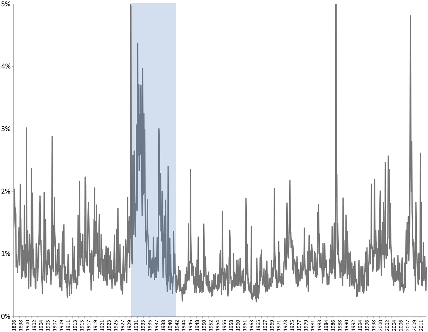
Figure 1. Stock volatility, 1896–2012
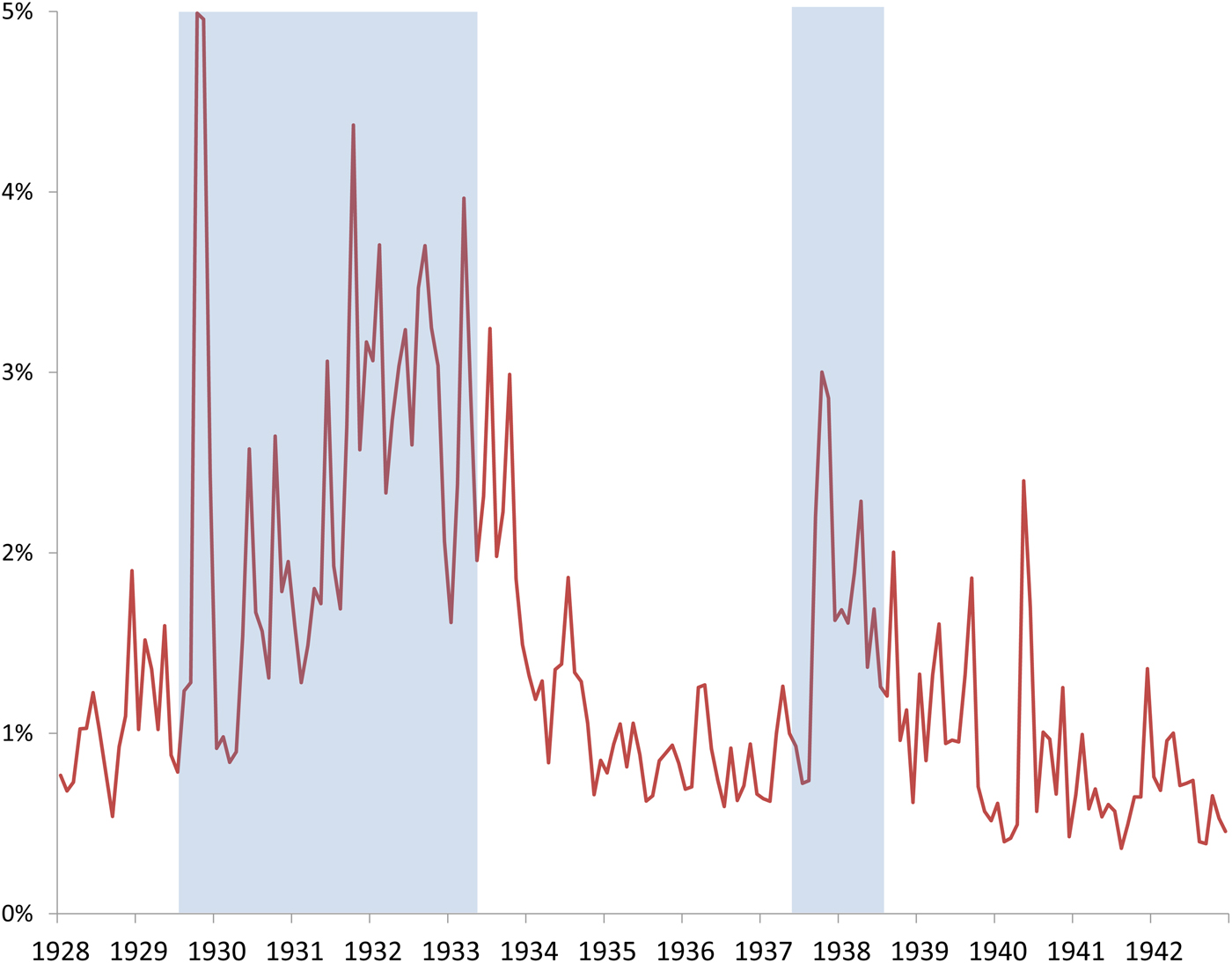
Figure 2. Stock volatility, 1928–42
Table I. Daily percentage increases or decreases in Dow Index, 1896–2013

Notes: Daily percentage return is daily change in log price of Dow Jones Industrial Average. Dates in bold indicate occurrence during 1929–33 NBER recession.
I define an uncertainty shock as an increase in the dispersion (second moment) of expected future outcomes. In a Knightian framework (Knight Reference Knight2012) uncertainty shocks, as defined here, would be closer in spirit to the concept of Knightian risk where probabilities are known but outcomes become more dispersed. There is also the concept of Knightian uncertainty where probabilities cannot be assigned to future outcomes, such as in Ilut and Schneider (Reference Ilut and Schneider2014), which is based on ambiguity aversion as in the famous Ellsberg Paradox (Ellsberg Reference Ellsberg1961). This class of models is less tractable, though obviously very relevant to real-world discussions of uncertainty.
In a financial context, uncertainty shocks express themselves either as uncertainty over future profitability or as uncertainty over the determinants of future discount rates, both of which will appear as increase return volatility. Dixit and Pindyck and their coauthors have produced an extensive literature on investment under uncertainty.Footnote 2 In general in these models, firms face uncertainty over revenue and costs when making an irreversible investment. As some future states of the world can be characterized by low profits, firms delay investment (McDonald and Siegel Reference McDonald and Siegel1986). I follow Schwert's characterization of stock market volatility as directly reflecting economic uncertainty: ‘[T]he volatility of stock returns reflects uncertainty about future cash flows and discount rates, or uncertainty about the process generating future cash flows and discount rates’ (Schwert Reference Schwert1989, p. 85). But it is not simply the case that this volatility is driven by a smooth process of regular increases or decreases in returns. New information or ‘news’ about uncertainty arrives periodically, and this drives discontinuous jumps in stock returns that can be observed during a period of uncertainty, such as the 1930s.Footnote 3
Veronesi (Reference Veronesi1999) develops a financial model with a regime shift between high and low economic uncertainty which produces significant variation in stock volatility over time. This model provides a theoretical justification for the stylized fact of a high correlation between uncertainty and stock volatility. Following the intuition in Veronesi (Reference Veronesi1999), I argue that uncertainty shocks will correspond to periods of high volatility, as uncertainty over the expected profitability of firms generates high stock volatility.Footnote 4 Volatility in discount rates would also generate higher stock volatility, as asset prices are determined jointly by discount rates and expected returns. This theory is both able to explain why stock returns made large upwards and downward movements as well as explaining the persistently high volatility through uncertainty, as this is a prediction of uncertainty theory. This argument can also help to explain why the American economy was in recession during these periods, as these uncertainty shocks would have reduced investment and consumption, which fell sharply during the Depression. To confirm the correct identification of uncertainty shocks from the historical record, I use the bipower variation test of Barndorff-Nielsen and Shephard (Reference Barndorff-Nielsen and Shephard2006) to show that not only was stock volatility high, but also the level of stock returns was constantly gyrating in large upward and downward jumps at the same time. There are some periods with low uncertainty and high volatility, such as the late 1990s, which see both high stock volatility and low jumps, as compared to the 1930s which sees high volatility and many discontinuous jumps. I then analyze the historical record to show the types of events that could have given rise to high uncertainty during the periods when output was falling in the 1930s.
An implication of the theory of investment under uncertainty, as in Dixit and Pindyck (Reference Dixit and Pindyck1994), is that periods of high uncertainty should cause firms to postpone investment and consumers to postpone consumer durable purchases. As Bernanke (Reference Bernanke1983) argued, if enough consumers and firms postpone these expenditures, then aggregate expenditures would fall and a recession would result. Both measures of volatility are high during the 1929–33 and 1937–8 recessions, which makes it plausible that uncertainty shocks played a role in these declines. This article examines the historical record of this period to outline a series of events that are candidates for uncertainty shocks, and then matches these events to change in stock returns and stock volatility, as predicted by the theory of investment under uncertainty.
The rest of the article proceeds as follows. Section ii outlines the test for stock return jumps using bipower variation. Section iii outlines events in the 1930s that could have driven these large increases in volatility and large increases in extreme jumps in stock returns. Section iv concludes.
II
While a Gaussian distribution roughly matches the distribution of stock returns in the data, the distribution of stock returns for the Dow Jones Industrial Average for 1896–2013 deviates significantly from a normal distribution. There remain ‘fat tails’, where the frequency of very large negative downward changes (and to some extent upward changes) in stock returns are larger than would be predicted with a normal distribution. To better model the distribution of stock returns, I will include a series of discontinuous ‘jumps’ which will arrive at a Poisson rate. This jump-diffusion model of stock returns has a long history in the literature, beginning with Merton (Reference Merton1976) and continuing with models like that of Kou (Reference Kou2002). The 1930s, especially during the 1929–33 Great Collapse period, saw many of the largest declines in the Dow Jones Industrial Average, but this period also saw some of the largest gains in Dow history as well. These results are plotted in Table 1, which shows clearly that this period saw both large downward and upward swings in the stock market. While assuming a Gaussian distribution is convenient, one can understand both the behavior of stock returns as well as how new information about uncertainty affects financial markets by examining discontinuous jumps, which are an important determinant of overall return volatility.
To separately identify jumps in the data from large observations of the diffusion part of the data-generating process, I use the bipower variation test of Barndorff-Nielsen and Shephard (Reference Barndorff-Nielsen and Shephard2006), which identifies jumps in a jump-diffusion time-series. There are many alternative methods of testing for jumps, but I chose this method as it is prominent in the literature and also because of the limited number of high-frequency (daily) series available for this period. If other high-frequency data were available, the preferable method of cojumping of Dungey and Martin (Reference Dungey and Martin2007), Dungey et al. (Reference Dungey, McKenzie and Smith2009), Dungey and Hvozdyk (Reference Dungey and Hvozdyk2012), Dungey and Gajurel (Reference Dungey and Gajurel2014), Claus and Dungey (Reference Claus and Dungey2016) would be a superior way to test for jumps. While there are other jump tests, such as Lee and Mykland (Reference Lee and Mykland2008), Mancini and Renò (Reference Mancini and Renò2011), Andersen et al. (Reference Andersen, Dobrev and Schaumburg2012), I chose the BNS test due to its frequent use among financial practitioners, as well as the straightforward and transparent way the statistics are calculated.
These jump-diffusion processes combine the standard Brownian diffusion process with a jump process as follows:
 $$\displaystyle{{dY_t} \over {Y_t}} = \eta dt + \sigma _t dW + xdZ.$$
In this continuous-time framework Y is the stock index level, η is the trend as a percentage, σ is the standard deviation of changes, x is the average size of discrete jumps, dW is a standard Brownian motion process which follows a Gaussian distribution, and dZ follows a Poisson distribution and has a value of either 0 or 1.
 $$[Y]_t = {\rm plim}\sum\limits_{\,j = 0}^{n - 1} (Y_{t,j + 1} - Y_{t,j} )^2 $$
and it is easy to show that [Y]
t
= [Y
c
]
t
+ [Y
d
]
t
, with $[Y^d ]_t = \sum\limits_{0 \le g \le t} \Delta Y_u^2 $
, and with ΔY
t
representing the jumps in Y. The null hypothesis of no jumps is formed by setting [Y] = [Y
c
]. While there is a limiting case of continuous time, my dataset uses daily data so I will perform the test with daily returns, defined as y
t
= Y
t
− Y
t−1. For daily returns, the bipower variation [1,1] of a time-series over time t is defined as follows:
$[Y^d ]_t = \sum\limits_{0 \le g \le t} \Delta Y_u^2 $
, and with ΔY
t
representing the jumps in Y. The null hypothesis of no jumps is formed by setting [Y] = [Y
c
]. While there is a limiting case of continuous time, my dataset uses daily data so I will perform the test with daily returns, defined as y
t
= Y
t
− Y
t−1. For daily returns, the bipower variation [1,1] of a time-series over time t is defined as follows:
 $$Y_t^{[1,1]} = \sum\limits_{\,j = 2}^t \vert y_{\,j - 1} \vert \vert y_j \vert $$
Barndorff-Nielsen and Shephard (Reference Barndorff-Nielsen and Shephard2004) show that the above expression can be consistently estimated with
 $$[Y]_t - (\mu ^{ - 2} )Y_t^{[1,1]}, $$
where $\mu = \sqrt {\displaystyle{2 \over \pi}} $
. The above expression is simply the difference between the bipower variation and the quadratic variation, and will provide the basis for the BNS difference test.
$\mu = \sqrt {\displaystyle{2 \over \pi}} $
. The above expression is simply the difference between the bipower variation and the quadratic variation, and will provide the basis for the BNS difference test.
To test for the presence of jumps in a time series, an estimator of integrated quarticity $\int_0^t \sigma _u^4 du$
is required. BNS propose quadpower variation, which is defined as follows:
$\int_0^t \sigma _u^4 du$
is required. BNS propose quadpower variation, which is defined as follows:
 $$Y_t^{[1,1,1,1]} = \sum\limits_{\,j = 4}^t \vert y_{\,j - 3} \vert \vert y_{\,j - 2} \vert \vert y_{\,j - 1} \vert \vert y_j \vert $$
The BNS difference test statistic has the following asymptotic distribution for daily returns.Footnote 5
 $$\hat D = \displaystyle{{\left(\mu ^{ - 2} \{ Y\} _t^{[1,1]} - [Y]_t \right)} \over {\sqrt {\theta \mu ^{ - 4} \{ Y\} _t^{[1,1,1,1]}}}} \to ^L N(0,1)$$
There is also a ratio test that measures the ratio of quadratic variation to bipower variation.
 $$\displaystyle{{\{ Y\} _t^{[1,1]}} \over {\sqrt {\theta \{ Y\} _t^{[1,1]}}}} \left( {\displaystyle{{\mu ^{ - 2} \{ Y\} _t^{[1,1]}} \over {[Y]_t}} - 1} \right) \to ^L N(0,1)$$
Intuitively, bipower variation is generated by the absolute value of the return multiplied by the lag, while the quadratic variation is the absolute value of the return multiplied by itself. Thus the difference between the two will capture how much the absolute value of the return changes between one day and the next. As the point estimate is related to the second moment, the relevant standard error is related to the square, and thus is a fourth-order moment, which is the quadpower variation. I use the BNS difference test to determine jumps, so the difference between quadratic and bipower variation is plotted for the entire period in Figure 3, where the Depression period clearly appears as a period of significant and persistent jumps. Notice that this test statistic will appear as a large value for both upward and downward jumps, so both negative and positive jumps are evidence of jumps in the series. Table 2 shows the 20 largest jumps in Dow history, with those occurring in the recession period of 1929–33 in bold. One can see that jumps predominate in this Great Contraction period with uncertain events corresponding to these jumps, which the reader will notice are both positive and negative. Other events that correspond to very large jumps are the 1987 crash and the very uncertain period of October 2008, as well as the 1937 recession and some jumps related to the run-up to World War I.
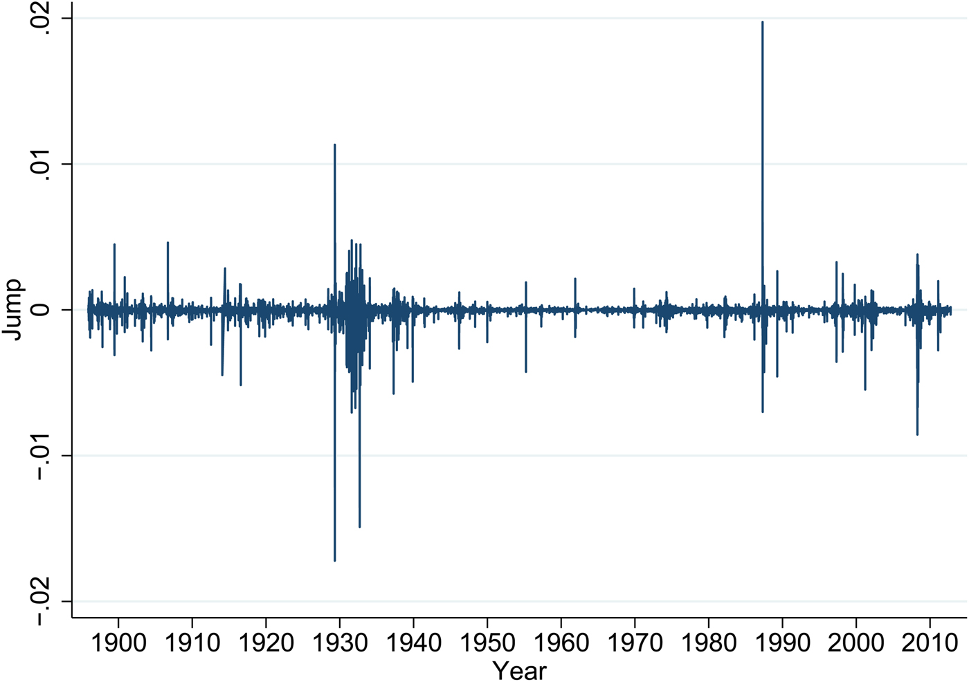
Figure 3. Jumps, 1896–2013
Table 2. Twenty largest jumps as measured by BNS jump test statistic, 1896–2013

Notes: Dates in bold indicate occurrence during 1929–33 NBER recession. Events derived from New York Times and Commercial and Financial Chronicle. BNS test statistic outlined in Barndorff-Nielsen and Shephard (Reference Barndorff-Nielsen and Shephard2006).
I perform both the BNS difference test as well as the BNS ratio test using daily return data from the Dow Jones Industrial Average from 1896 to 2013.Footnote 6 The tests yield very small p-values, so I can reject the null hypothesis of no jumps in the series for both the entire sample of 1896–2013 as well as the 1929–41 Great Depression period. For the BNS difference test, I obtain a Z-value of −6.43 for the entire period, and −3.22 for the Great Depression, with both p-values significant at the 0.1 percent level. For the BNS ratio test, I obtain a Z-value of −3.224664 for the entire sample and a Z-value of −2.817148 for the Great Depression, with both tests recommending rejection at a 1 percent level. Thus the BNS tests clearly point to the existence of jumps. Bloom (Reference Bloom2009) also performs the BNS difference and ratio tests, and finds support for jumps in return for the postwar as I do for the interwar period.
I also display in Figure 4 the percentage of the month that features ‘high jumps’, which I define to be in the 95th percentile of jumps over the entire period. A comparison to the policy uncertainty index of Baker et al. (Reference Baker, Bloom and Davis2015), based on newspaper mentions of policy uncertainty, is featured in Figure 5, scaled to be comparable. While the economic policy uncertainty index is higher during the New Deal period of 1934–41 before the war, the jump series is higher during the recessionary periods of 1929–33 and 1937–8, perhaps reflecting the prominent discussion of uncertainty in the newspaper on which the policy uncertainty index is based, relative to the actual impact of financial markets in the jumps measure. It is plain to see that the period with many jumps is also the period when stock volatility is high, which is consistent with the uncertainty hypothesis where stock prices should exhibit large returns jumps and high stock volatility during uncertainty periods. Recession periods are also indicated, which are contemporaneous with the periods of high jumps, which is consistent with uncertainty shocks generating both discontinuous jumps and these sharp recessions.
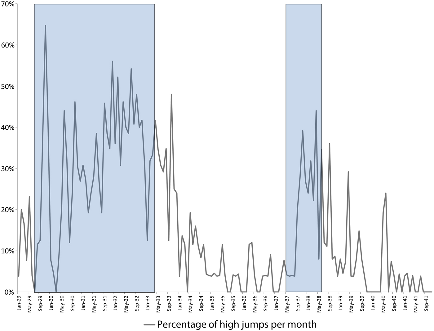
Figure 4. Jump percentage, 1929–38
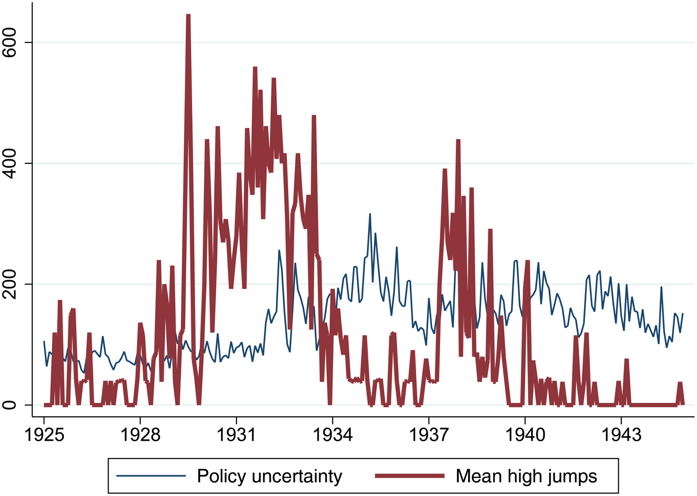
Figure 5. Comparison of economic policy uncertainty index and large jumps
III
Bloom (Reference Bloom2009) points to major uncertainty shock events in the postwar era which coincided with major stock volatility and significant uncertainty such as the Cuban missile crisis, the assassination of John F. Kennedy, the Gulf War, the Asian financial crisis, 9/11 and the 2008 financial crisis. In a related paper, Charles and Darné (Reference Charles and Darné2014) identify large shocks in the volatility of the Dow Jones Industrial Average from 1928 to 2013 and, similarly, find that both the 1929–34 and 1937–8 periods see elevated return volatility. Moreover, these authors use a similar narrative approach to match large jumps to particular events, though they do not make the explicit connection to uncertainty and do not analyze some lower-frequency increases in uncertainty such as banking failures and the possibility of an end to the capitalist system.
Using historical print sources, primarily books and articles from publications like the Commercial and Financial Chronicle and the New York Times, I construct a timeline of Depression uncertainty shock events in the same vein as these authors, which can be seen in Figures 6 and 7. All the events are listed in Table 3 with a corresponding classification of the uncertainty shock type, which matches these events to large jumps and stock volatility during the 1929–41 Great Depression. Naturally this narrative is somewhat subjective and other interpretations of the historical record are possible, but I have done my best to present an unbiased timeline that helps explain the behavior of asset prices during this period through the lens of the theory of uncertainty shocks.
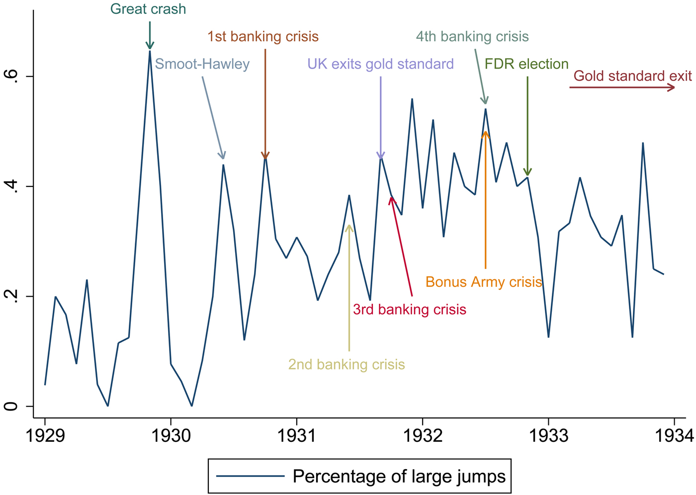
Figure 6. Large jump events, 1929–33. Large jumps are the largest 5 percent of jumps in the sample as calculated by BNS difference test (Barndorff-Nielsen and Shephard Reference Barndorff-Nielsen and Shephard2006). Percentage of large jumps is the ratio of number of days with large jumps to total days in month.
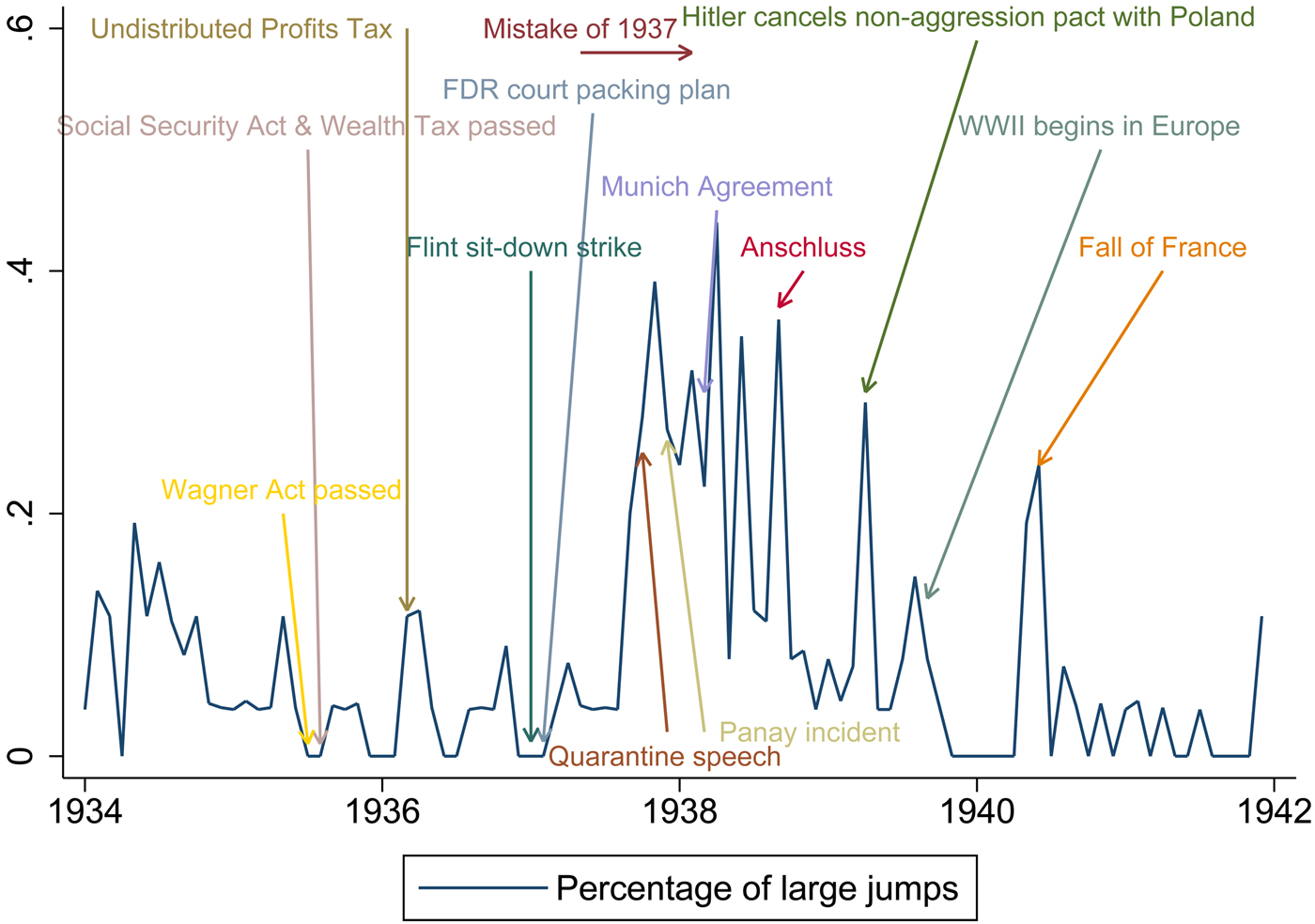
Figure 7. Large jump events, 1934–8. Large jumps are the largest 5 percent of jumps in the sample as calculated by BNS difference test (Barndorff-Nielsen and Shephard Reference Barndorff-Nielsen and Shephard2006). Percentage of large jumps is the ratio of number of days with large jumps to total days in month.
Table 3. Uncertainty shock events

The roots of the crisis of 1929 can be found in the economic and asset boom that preceded the crash. In order to combat stock market speculation and a stock market bubble, the Federal Reserve raised discount rates to discourage stock buying using margin borrowing and to prevent the economy from overheating (Eichengreen Reference Eichengreen1996). While this action slowed output growth, its effect were debated for a long period at the Fed and the discount rates were relatively well communicated relative to other monetary policy at the interwar Fed. The United States eventually did experience a mild downturn, as the peak of industrial production and the official start of the recession can be dated to the summer of 1929.Footnote 7 Up to this point, I see no role for uncertainty as an explanatory factor in the nascent disaster. Monetary tightening, as outlined in Hamilton (Reference Hamilton1987), is sufficient to explain the mild decline in economic activity.
Most likely due to the unsustainable rise of securities prices between 1928 and 1929, stocks crashed in October 1929 in one of the largest financial routs in American history. In the wake of this stock crash, the character of the downturn changed significantly. However, while the recession may have appeared to be mild to observers at the time, the Great Crash of 1929 would fundamentally change the nature of the downturn, as Friedman and Schwartz argue:
During the two months from August 1929 to the crash, production, wholesale prices, and personal income fell at annual rates of 20 percent, 7.5 percent, and 5 percent, by October respectively. In the next twelve months, all three series fell at appreciably higher rates: 27 percent, 13.5 percent, and 17 percent, respectively. All told, by October 1930, production had fallen 26 percent, prices, 14 percent, and personal income, 16 percent … Even if the contraction had come to an end in late 1930 or early 1931, as it might have done in the absence of the monetary collapse that was to ensue, it would have ranked as one of the most severe contractions on record. (Friedman and Schwartz Reference Friedman and Schwartz1971, p. 306)
Friedman and Schwartz are well known for their monetarist explanation for the Great Depression. But one important, perhaps underappreciated, aspect of their argument is the central role that uncertainty plays in their monetary theory of the Depression. Friedman and Schwartz argue, as Romer (Reference Romer1990) does, that uncertainty was a direct result of the Great Crash of 1929.
Partly, no doubt, the stock market crash was a symptom of the underlying forces making for a severe contraction in economic activity. But partly also, its occurrence must have helped to deepen the contraction. It changed the atmosphere within which businessmen and others were making their plans, and spread uncertainty where dazzling hopes of a new era had prevailed. It is commonly believed that it reduced the willingness of both consumers and business enterprises to spend, … (Friedman and Schwartz Reference Friedman and Schwartz1971, p. 306)
Romer (Reference Romer1990) examined contemporary business forecasts, which became markedly more uncertain after the crash. While monetary factors were most likely another trigger for the price collapse, the Great Crash generated a sense of uncertainty among businesses and consumers. After October 1929 stock volatility and return jumps fell significantly, such that these uncertainty measures are low by early 1930. However, the largest declines in the DJIA in US history occur on 28 and 29 October and 6 November, with declines of 12.82, 11.73 and 9.92 percent respectively.Footnote 8 Contrary to the popular misconception that the Great Crash was a single day's decline, October 1929 actually saw several days of extreme jumps. Moreover, the third largest increase in Dow Jones history occurred on 31 October when some investors purchased stocks in a wave of optimism.
Several events that generated euphoria and disappointment are evident from both Table 1, which lists the largest daily returns, and Table 2, which lists the largest jumps in Dow history.Footnote 9 On 14 November 1929, a discount rate cut by the New York Federal Reserve from 5 to 4.5 percent sparked optimism that the crash of the month before would not last (Friedman and Schwartz Reference Friedman and Schwartz1971, p. 367) and led to a 10 percent increase in the Dow. On 6 October 1931, the Dow Jones surged higher by over 12 percent, the fifth highest jump in US history, despite coming in the wake of the UK departure from the gold standard and another wave of banking failures. On that date, President Hoover outlined a plan for a banking coalition to improve confidence in the banking system, which led to optimistic buying (Hoover Reference Hoover1931).
On 11 February 1932, the resignation of Hoover's liquidationist Treasury Secretary, Andrew Mellon, generated a wave of optimism that the economy would improve as a result of his resignation, which caused a large jump in stocks and the ninth largest jump in US history.Footnote 10 On 3 August 1932, the Dow rose almost 10 percent on the news that General Motors would pay a dividend again after a long suspension, which pointed some towards expectations of recovery. On 12 August 1932, the DJIA fell by over 8 percent after Herbert Hoover accepted to be the Republican nominee in 1932, with the prospect that his ineffective policies would continue.
On 10 June 1932 Congressman Louis McFadden gave a speech that blamed the Federal Reserve and Wall Street for the Depression, which raised the prospect of increased regulation and scrutiny of the financial system. On 21 September 1932, the Dow rose by over 11 percent, the eighth largest jump, on the news that the Reconstruction Trust Finance Corporation, a government agency meant to support the banking system, would support agriculture as well. The largest daily return (an increase of 15.34 percent) occurred on 15 March 1933 when the Emergency Banking Act and the bank holiday ended. As these programs were concluded successfully, only solvent banks remained. This decisively ended the banking panics of the early 1930s and investors could expect a much more profitable future (Friedman and Schwartz Reference Friedman and Schwartz1971).Footnote 11
Wicker (Reference Wicker2001) identifies four major periods of banking crises, which largely line up with the banking crises identified by Friedman and Schwartz (Reference Friedman and Schwartz1971). These banking crises took place from November to December 1930, April to August 1931, September to October 1931 and June to July 1932.Footnote 12 It is intuitive that large-scale bank failures would reduce confidence about the future. Bank runs and uncertainty about whether one's life savings would be safe could only have added to the existing uncertainty. Friedman and Schwartz argued that the increase in uncertainty in the 1930s could explain the decline in monetary velocity. In this theory, economic agents would hold money due to a ‘precautionary savings’ effect, which is quite similar to a real-option effect due to uncertainty at the firm level.
Other things being the same, it is highly plausible that the fraction of their assets individuals and business enterprises wish to hold in the form of money, and also in the form of close substitutes for money, will be smaller when they look forward to a period of stable economic conditions than when they anticipate disturbed and uncertain conditions … The more uncertain the future, the greater the value of such flexibility and hence the greater the demand for money is likely to be. (Friedman and Schwartz Reference Friedman and Schwartz1971, p. 673)
Thus we have another channel whereby uncertainty can reduce aggregate demand, through a monetary channel in this case. ‘The contraction instilled instead an exaggerated fear of continued economic instability, of the danger of stagnation, of the possibility of recurrent unemployment. The result, from this point of view, was a sharp increase in the demand for money, accounting for the magnitude of the decline in velocity from 1929 to 1932’ (Friedman and Schwartz Reference Friedman and Schwartz1971, p. 673). Cole and Ohanian (Reference Cole and Ohanian2001) find that the banking collapse was not a major factor in the decline of output from 1929 to 1933, as only 0.4 percent of banking deposits were lost from 1930 to 1932, which was similar ratio as for the 1920–1 recession. Also, Cole and Ohanian (Reference Cole and Ohanian2001) are not able to generate a significant decline in output as a result of banking failures from their general equilibrium model. However, while the direct effect of these banking failures may not be very large, the uncertainty effect of banking failures on household behavior could still be sizeable. For example, uncertainty over potential banking failures caused households to pull their money out of banks and reduced monetary velocity. Thus the Friedman–Schwartz monetary hypothesis can be seen through an uncertainty lens where the sharp decline in velocity is due, in large part, to these uncertainty shocks.
While tariffs did rise astronomically in the wake of the Smoot–Hawley Tariff, the direct impact was clearly too small to have been a primary explanation for the Great Depression (Eichengreen Reference Eichengreen1988). However, this tariff could have a significant uncertainty effect, as argued by Archibald and Feldman (Reference Archibald and Feldman1998) and discussed in the Wall Street Journal.Footnote 13 Indeed, there is a spike in stock volatility in June 1930 when the Smoot–Hawley tariff was signed into law. Also, the extent of retaliation by American trading partners was uncertain: would other countries raise tariffs on American products? Canadian tariffs did rise significantly over this period in retaliation. Elsewhere nominal tariffs rose quickly, and volatile and unpredictable deflation made real tariff rates uncertain (Hamilton Reference Hamilton1992). While the Smoot–Hawley tariff was not a large uncertainty event on its own, it is plausible that this major policy change increased uncertainty. Indeed, the Dow Jones Industrial Average fell by 6 percent on 16 June when passage of the Smoot–Hawley Tariff was assured.
While in hindsight it is clear that the end of the gold standard was necessary for recovery (Eichengreen Reference Eichengreen1996), during the Depression the ‘gold standard mentality’ was prevalent (Mouré Reference Mourè2002); countries would stay on the gold standard until the costs became too much to bear. This happened to the United Kingdom in September 1931, and jumps increased during this month. It was unclear whether the British departure would drive the United States to leave the gold standard as well. As gold flowed to the UK the money supply in the United States fell and a financial and banking crisis resulted. In response, the Fed raised interest rates to preserve the gold standard, though of course this further worsened the negative effects of the financial crisis. Ferderer and Zalewski (Reference Ferderer and Zalewski1999) find that uncertainty propagated the Great Depression as doubts about a country's commitment of the gold standard lead to interest rate volatility, which then results in output declines; this channel can be seen in operation in September 1931.
The Great Depression brought widespread hunger and unemployment, so it is perhaps unsurprising that support for radical policies grew. A Roman Catholic priest, James Cox, led 25,000 unemployed Pennsylvanians on a march on Washington in January 1932 to push for increased relief for the unemployed and stronger labor unions. This was a prelude for the much larger Bonus Army marches of the spring and summer. Veterans of World War I were promised, through 1924 legislation, a Veteran's Bonus, to be paid in 1945. Widespread unemployment and poverty among veterans during the 1930s drove a push by veterans' groups for the bonus to be paid early, and some 17,000 veterans and their families went to Washington to lobby the government. Media reports claimed that the veterans' groups were largely composed of communists and criminals. General MacArthur saw the marchers as revolutionaries intent on overthrowing the Republic, a sentiment with which Patrick J. Hurley, the Secretary of War, enthusiastically agreed (Lisio Reference Lisio1967).
While these sentiments may have been overblown, the perceived probability of violence and radicalism among well-trained veterans in the heart of the nation's capital could not but generate a sense of uncertainty. The eviction of the Bonus Army on 28 July coincides with a substantial increase in the percentage of large jumps. The eviction began with two marchers being killed by police. As the crisis intensified, MacArthur commanded a tank column, ordering a cavalry charge and infantry armed with bayonets and vomiting gas to disburse the veterans (Dickson and Allen Reference Dickson and Allen2006).Footnote 14 On 5 October 1932, the Minnehaha County Farmers' Holiday Association, a farmers' organization, blocked roads in Sioux Falls to protest low agricultural prices. Their blockade was part of a supply-side boycott of farmers refusing to sell their farm products until prices rose to protect agricultural surpluses. These Farm Holiday Associations threatened significant rural unrest, in keeping with the general instability of the time, and this event coincided with a major jump in the Dow Index.
Uncertainty resulting from the gold standard's future was discussed in the context of the British departure from gold in 1931. Friedman and Schwartz also saw significant uncertainty in 1933 regarding the status of the gold standard in the United States under a Roosevelt administration:
The rumors about gold were only one part of the general uncertainty during the interregnum about future financial and economic policy. Under ordinary circumstances, it would have been doubtful that such rumors and such uncertainty would be a major force accounting for so dramatic and widespread a financial panic. But these were not ordinary circumstances. The uncertainty came after more than two years of banking difficulties in which one wave of bank failures had followed another and had left the banking system in a particularly vulnerable position. The Federal Reserve itself participated in the general atmosphere of panic. Once the panic started, it fed on itself. (Friedman and Schwartz Reference Friedman and Schwartz1971, p. 332)
Roosevelt did not initially have a clear position on the gold standard, so there was some uncertainty over his potential gold standard policies during the election. This uncertainty can be seen during his inauguration as president (March 1933), at the time of Executive Order 6102, which forced the sale of private gold holdings to the government (April 1933), and the Gold Reserve Act (January 1934), which set gold's price at $35 an ounce.Footnote 15 The gold price floated between March 1933 and January 1934, the period during which there are the largest jumps in returns; this could be due to lingering uncertainty over the gold standard prior to the repegging of the dollar at the rate of $35 per troy ounce. The Gold Reserve Act also set up an Exchange Stabilization Fund, which purchased gold in exchange for freshly created money; this put in place a more clearly expansionary monetary policy (Wicker Reference Wicker1971).
For Friedman and Schwartz, monetary policy can work better if it is not impeded by the negative impacts of uncertainty. ‘After three years of economic contraction, there must have been as many forces in the economy making for revival, and it is reasonable that they could more readily come to fruition in a favorable monetary setting than in the midst of continued financial uncertainty’ (Friedman and Schwartz Reference Friedman and Schwartz1971, p. 324). While this study does not address the interaction between uncertainty and monetary policy effectiveness, Vavra (Reference Vavra2013) and Bloom et al. (Reference Bloom, Bond and Van Reenen2007) found monetary policy was less effective during volatile or uncertain times, confirming Friedman and Schwartz's intuition. This lingering uncertainty at the beginning of the recovery can help explain why recovery was not more rapid given the sharp change in monetary policy from contractionary to expansionary. Other policies, like the National Industrial Recovery Act (NIRA), represented major departures from existing policy and significant interventions in the American economy of the time (Cole and Ohanian Reference Cole and Ohanian1999).
Support for existing political and economic frameworks receded during the 1930s. With widespread hunger and unemployment, it is perhaps unsurprising that support for radical policies and actions rose. This rising tide of populism naturally made business uncertain about its future prospects. Merton (Reference Merton1985, p. 1185) also argued that there was significant uncertainty about the survival of capitalism: ‘With the benefit of hindsight, we know that the US and world economies came out of the Depression quite well. At the time, however, investors could not have had such confident expectations.’Footnote 16 Voth (Reference Voth2002) found that stock volatility and uncertainty rose during waves of strikes and other political uncertainty in Europe, where the threats of upheaval and violence were tragically realized. The Roosevelt administration was well aware of the threats of upheaval they faced. Franklin Delano Roosevelt (FDR) remarked to John Nance Garner, his vice-president, on the way to his inauguration: ‘I had better be a good president or I will be the last one’ (Cowley Reference Cowley1981, p. 152) Other observers shared these sentiments:
Before March 4th, America was in a state of extreme shock. No one would ever know, General Hugh S. Johnson later said, ‘how close were we to collapse and revolution. We could have got a dictator a lot easier than Germany got Hitler.’ ‘I do not think it is too much to say,’ wrote Tugwell, ‘that on March 4 [Roosevelt's inauguration] we were confronted with a choice between an orderly revolution – a peaceful and rapid departure from past concepts – and a violent and disorderly overthrow of the whole capitalist structure.’ (Schlesinger Reference Schlesinger2003b, p. 22)
This was not idle speculation. General Smedley Butler, who had been active with the Bonus Army, would later be approached by a group of executives and conservatives opposed to Roosevelt. The plan of the ‘Business Plot’ was to have Butler lead a veterans' group in overthrowing Roosevelt and imposing a authoritarian government more favorable to opponents of the New Deal. While this plot was largely ridiculed at the time and even today, when Butler testified in 1934 an official government investigation found these allegations to be true (Schlesinger Reference Schlesinger2003b). Farmers were also hard-hit by the Depression and this discontent could have easily become violent had the farm crisis not been resolved.
The seething violence in the farm belt over the winter – the grim mobs gathered to stop foreclosures, the pickets along the highways to prevent produce from being moved to town – made it clear that patience was running out. In January 1933, Edward A. O'Neal, the head of the Farm Bureau Federation, warned a Senate committee: ‘Unless something is done for the American farmer we will have revolution in the countryside within less than twelve months.’ (Schlesinger Reference Schlesinger2003b, p. 28)
While it is difficult to point to specific events where the possibility of regime change was more salient, stock volatility and return jumps are high during the period 1929–34 when this uncertainty was more salient, and after 1934 when recovery was taking hold and support for existing political and economic structures rose, uncertainty fell as well.
Criticism of Roosevelt was prevalent in the 1930s, as the election of 1932 brought to power an executive and legislative branch that was highly supportive of an expanded role of government in the economy. This unprecedented government intervention in the economy was opposed by critics like the ‘Old Right’ as moves towards socialism or fascism (Hoover Reference Hoover1952). Schumpeter argued that the major legislative changes caused uncertainty about the path and effects of government policy.
The subnormal recovery to 1935, the subnormal prosperity to 1937 and the slump after that are easily accounted for by the difficulties incident to the adaptation to a new fiscal policy, new labor legislation and a general change in the attitude of government to private enterprise all of which can be distinguished from the working of the productive apparatus as such. So extensive and rapid a change of the social scene naturally affects productive performance for a time, and so much the most ardent New Dealer must and also can admit. I for one do not see how it would otherwise be possible to account for the fact that this country which had the best chance of recovering quickly was precisely the one to experience the most unsatisfactory recovery. (Schumpeter [1942] 1994, pp. 64–5)
This ‘regime uncertainty’ argument has continued to influence modern scholars. Higgs (Reference Higgs1997) argues that the uncertainty regarding private property rights during the Roosevelt administration explains the weak investment seen during the 1930s. As policies were unclear, business did not want to invest given the uncertain future. This is similar to the ‘wait-and-see’ effect discussed earlier. Higgs lists some events that could have generated regime uncertainty, but this is simply a list of New Deal policies and does not identify more or less important policies. I will focus on major New Deal legislation that had significant implications for the economy, to see if these events acted as uncertainty shocks.Footnote 17 Endogeneity may be a concern here as the economic downturn, partially driven by the uncertainty of 1929–33, played a big role in the New Deal landslide of 1932, and thus the downturn could have generated some uncertainty. However, Baker and Bloom (Reference Baker and Bloom2013) show that natural disasters, clearly exogenous events, generate declines in output through the channel of uncertainty, addressing this endogeneity issue, though Bloom (Reference Bloom2013) finds that uncertainty is, to some extent, endogeneous.
Roosevelt's first hundred days saw a unprecedented amount of legislation introduced by New Deal supporters who dominated both the executive and legislative branches. The Federal Emergency Relief Administration (FERA) expanded federal anti-poverty programs, the AAA greatly expanded federal intervention in agricultural markets to aid farmers, and the RFC started to purchase the banking shares of troubled banks, while Roosevelt's bank holiday shuttered all banks temporarily to try to weed out insolvent banks. All of these changes are often pointed to as a primary cause of elevated uncertainty during this period. In terms of generating a sense of uncertainty, the NIRA is perhaps the clearest candidate. This Act put in place the National Recovery Administration (NRA) in June 1933. This allowed business to collude and set minimum standards for wages and prices. Thousands of pages of codes were printed to regulate almost all aspects of business. Adding to the uncertainty was doubt over the constitutionality of the bill. This uncertainty was resolved in 1935 when the Supreme Court struck down the NIRA in Schechter Poultry Corp. v. United States. The ruling of the NIRA as unconstitutional on 27 May 1935 would seem to return the American economy to a more familiar regulatory framework. If the regime uncertainty hypothesis were correct, uncertainty, as measured by stock volatility, should decrease as the regulatory regime became more certain. However, no change in large jumps is observable, though that may be because the NIRA had already stopped being effective months before.Footnote 18
The Wagner Act, which was signed into law on 5 July 1935, was the high tide for union legislation in American history. This Act constrained employer interference in union activities and encouraged collective bargaining and the right to strike. The number of strikes increased dramatically after the passage of this Act, and it seems plausible that this Act could have increased uncertainty in affected industries. The Revenue Act of 1935 also raised taxes significantly, and was called a ‘Soak the Rich’ tax. By February 1937 the United Auto Workers' strike in Flint, Michigan, had succeeded and the union was recognized by General Motors, a major coup for the labor movement. The Social Security Act, following soon after the Wagner Act's passage on 14 August 1935, heralded a major expansion of social spending by the federal government and set the stage for vastly higher tax rates. In June 1936, an Undistributed Profits Tax was imposed, which encouraged businesses to distribute profits as dividends instead of retained earnings. By reducing undistributed profits, this tax made bankruptcy much more likely for firms in trouble as they had fewer cash reserves (Hendricks Reference Hendricks1936). In his fireside chat of 9 March 1937, Roosevelt announced his intention to ‘pack’ the Supreme Court by adding more judges to the court. This policy would allow the president to appoint judges favorable to the New Deal to the court. This was ultimately unsuccessful, though the attempt was widely viewed as an overreach by the executive.
Many of these New Deal events are shown in Figure 7. Other than the NIRA's passage none of these events line up with high volatility and jumps, which were vastly reduced from the volatile period of 1929–34. While policy uncertainty could absolutely create uncertainty shocks, the evidence doesn't show that policy uncertainty played a large role in the weak recovery. Uncertainty was falling while real GDP growth was growing at record rates while the New Deal was in place, as pointed out by Eggertsson (Reference Eggertsson2010, p. 203). Similarly, Roose (Reference Roose1969, p. 225) argues that given the conservative victories of 1936, the regime uncertainty argument would have predicted a large boom rather than the recession that followed.
Romer (Reference Romer1992) argues that the recovery was not slow, as GDP growth rates were at a record high for peacetime. Also, the focus on the potential for an even stronger New Deal recovery seems misplaced, as the economy effectively reached its trough in March 1933 when Roosevelt was inaugurated, and record declines in GDP under Hoover were replaced with record GDP growth rates for peacetime under Roosevelt. This article is the first both to directly address economic uncertainty in the New Deal and to find that the New Deal only generated uncertainty in its early phases through 1934 and not for the rest of the Roosevelt presidency.Footnote 19
It is clear that the devaluation of the dollar in 1933 was enormously beneficial to the American economy. The devaluation increased the value of the monetary gold stock, encouraged an inflow of gold from abroad and caused the price level to shoot up. Romer (Reference Romer1992) finds that stimulative monetary policy alone essentially explains the recovery from the Great Depression and Temin and Wigmore (Reference Temin and Wigmore1990) frame the devaluation as a major regime change with significant positive consequences. Eggertsson (Reference Eggertsson2008) argues that the devaluation fundamentally changed agents' expectations from deflationary to inflationary, due to both the devaluation and Roosevelt's commitment to reflate the price level back to its 1926 level. According to Eggertsson, the administration made this commitment credible by increasing real and nominal spending. Indeed, price-level targeting is a ‘fool-proof’ way to exit a liquidity trap according to Svensson (Reference Svensson2001), and the American economy did rapidly exit the liquidity trap after this regime change. Building on Eggertsson's analysis, I argue that this policy change had an effect beyond the direct monetary effect. The more important effect was that the increased credibility and commitment of these expansionary monetary policies vastly reduced uncertainty about future demand and profitability. Return volatility fell rapidly to more moderate levels from 1933 to 1937, after being high during the period when monetary policy was uncertain.
However, it is clear that from the gold standard suspension during the first hundred days, through the new parity of $35 per troy ounce of gold under the Gold Reserve Act of 1934, there was some uncertainty over the future of the American gold standard. Lewis W. Douglas, Roosevelt's Director of the Bureau of the Budget, minced no words in commenting on the suspension of the gold standard, ‘This is the end of Western civilization’ (Schlesinger Reference Schlesinger2003a, p. 201). Conservatives were concerned that these large monetary changes generated much uncertainty, which does find some confirmation in the extreme jumps of this period (Schlesinger Reference Schlesinger2003a, p. 200).
The recovery of the 1930s was not unbroken, as the American economy suffered a second recession between the summer of 1937 and the summer of 1938. The monetarist argument of Friedman and Schwartz (Reference Friedman and Schwartz1971) posits that monetary policy switched from being expansionary to being sharply contractionary in 1936–7 due to a misplaced fear of inflation, and that this policy change can explain the 1937–8 recession. Keynesian critics like Telser (Reference Telser2001) argue that, as the United States was at the zero lower bound, the banking system had significant excess reserves. This meant that increased reserve requirements could be met easily by reclassifying excess reserves as required reserves without restricting lending. Calomiris et al. (Reference Calomiris, Mason and Wheelock2011) and Park and Horn (Reference Park and Horn2015) find increases in required reserves have little effect on lending, while Cargill and Mayer (Reference Cargill and Mayer2006) find otherwise.
Eggertsson and Pugsley (Reference Eggertsson and Pugsley2006) argue that there is scope for monetary policy through a non-reserve channel, though they do cite the change in reserve policy and other policies like the Treasury's sterilization of gold as contributing to the downturn. For Eggertsson and Pugsley, Roosevelt had a clear policy of reflation and price-level targeting at the 1926 price level from 1933 to 1937. In 1937, he was convinced by his advisors that the economy was near recovery. Due to this belief and an inflation rate that was creeping higher, Roosevelt's administration abandoned its commitment to reflation and left policy vague and unclear. By 1938, the administration reversed its stance, and committed itself to its previous policy of reflation and price-level targeting at the 1926 price level. These policy changes, based on dates outlined in Eggertsson and Pugsley (Reference Eggertsson and Pugsley2006), show that policy changes that left policy unclear are associated with return jumps and volatility, while changes in policy that were clearly expansionary and more certain in 1938 are associated with lower volatility. I have noted in Figure 7 the period that Eggertsson and Pugsley highlighted as characterizing the ‘Mistake of 1937’, which is also a period when equity returns are very volatile and large jumps are observed.
While the 1937 recession was most likely sparked by monetary policy changes and associated monetary uncertainty, events in 1937 through 1939 related to the prospect of war in Europe and in the Pacific also generated heightened uncertainty. In retrospect, it may seem that the prospect of war would have been welcome given the record GDP growth of the war years to come. Indeed, the American economy had experienced an economic boom in the late 1910s during the Great War, especially in agriculture bolstered by agricultural exports. However, this boom led to a postwar surge in inflation and ultimately the painful recession of 1920–1. Sentiment was strongly opposed to foreign entanglements in the 1920s and 1930s, showing that the war was not seen fondly (Lowenthal Reference Lowenthal1981). Attacks on American shipping had been one of the triggers for the American declaration of war in 1917, and the Neutrality Acts of the 1930s made the prospects for international trade during the war dire, as discussed in the The Annalist.Footnote 20 Even if the United States remained neutral during the conflict, it could find itself cut off from export markets. The Neutrality Act of 1937 extended the existing embargo on arms to any warring nations, while extending the prohibitions to exclude belligerent ships from US ports. Any trade in non-military material could only occur on a ‘cash-and-carry’ basis, which meant payment had to take place immediately in cash. Any loans to or security exchange with belligerents was also banned (Fellmeth Reference Fellmeth1996).
Roosevelt had followed popular sentiment in supporting neutrality and publicly expressed an aversion to interventionism. His famous ‘I hate war’ speech of August 1936 was one of the more forceful examples of this. However, it is clear that he was supportive of the British side and wished to intervene on behalf of Britain and China in the case of armed conflict. In September 1937 Japan bombed major Chinese cities such as Shanghai and the War in the East began in earnest. In response to this, Roosevelt gave his famous Quarantine Speech in October 1937. He argued that ‘a reign of terror and international lawlessness’ by the fascists threatened peaceful nations everywhere. If this violence and war did not stop, other peaceful nations would be forced to act and ‘quarantine’ this threat. As this was not only a change in policy but an unclear one, observers at the time were not sure what to make of it. While Roosevelt had not officially repudiated neutrality, he did favor the Allies (Maney Reference Maney1998, p. 114). On 12 December 1937, the Japanese airforce bombed and sank the USS Panay in Nanking harbor. While Japan claimed this was accidental, American flags were clearly visible to Japanese pilots.Footnote 21 The business press reported on the connection between these uncertainty shocks and large gyrations in equity markets, e.g. the Annalist reported on stock declines in relation to tensions in Asia, and there was a similar article on uncertainty in the European situation and its relation to stock declines in the United States.Footnote 22
Conditions in Europe had worsened by 1937 and 1938 as well. On 11 and 12 March 1938, German soldiers invaded and annexed Austria into the Reich in the Anschluss. Emboldened by Allied weakness, Hitler immediately demanded the Sudetenland from Czechoslovakia. As both the USSR and France (and, by extension, potentially the United Kingdom) had treaty commitments to defend Czechoslovakia, tensions were high throughout September 1938. This crisis had the potential to set off a general war in Europe. Tensions remained high when Hitler canceled the non-aggression pact with Poland in April 1939, which eventually led to the September 1939 invasion of Poland, bringing the UK and France into World War II. Stock volatility was generally low from 1939 through December 1941 with the exception of the fall of France in 1940, which appears as a spike in large return jumps. Given the uncertainties that had prevailed in the early 1930s, it is perhaps unsurprising that business sentiment was sensitive to uncertainty, as Roose argues in his seminal analysis of the 1937–8 recession (Roose Reference Roose1969, p. 219).
IV
The Great Depression period has been extensively studied by both economists and historians due to its importance both as a macroeconomic event and as a watershed in American history. Previous accounts have focused mainly on monetary, fiscal or policy-related explanations for this unprecedented economic crisis. This article adds to the previous literature on the 1929–41 period by outlining major plausible uncertainty shocks in this period. Integrating the well-established connection between stock volatility and uncertainty, and utilizing the Barndorff and Nielsen-Shephard test for bipower variation to identify jumps in returns, this history was connected with economic theory regarding the effect of uncertainty on financial markets.
This article has also made the case that uncertainty shocks can be identified by information from securities markets, and that these uncertainty shocks are concentrated in the recession periods of the 1930s. Not only were prices and output falling during this period, but also we can see uncertainty shock events that correspond with these periods of equity volatility and extreme changes in returns as theory would predict. I find, contrary to the existing literature, that New Deal policy changes did not generate large increases in uncertainty, as can be seen by low levels of both overall stock volatility and these discontinuous jumps. Major drivers of both jumps and return volatility during the 1929–33 Great Contraction are primarily banking failures, the breakdown of the gold standard and the threat of an end to capitalism. While uncertainty plays a smaller role in 1938, monetary uncertainty and war jitters help explain this uncertain recessionary period as well. The Great Depression was an uncertain period, which can be seen in large and persistent disturbances to equity markets as well as in the economic collapse of that period.