


Impact Statement
The transition to turbulence from a laminar boundary layer is a major physical problem studied by the aeronautical industry because of the impact of the transition on the drag of an aircraft. In order to minimize it and to be more energy and cost efficient, laminar wings are designed. This type of wing is designed to adapt the pressure gradient generated by the wing aerodynamics in order to dampen the growth of instabilities (Tollmien–Schlichting and cross-flow waves) developing within the boundary layer. However, the presence of surface defects can induce an amplification of these unstable waves and a triggering of the turbulence. Tools that can predict the impact of surface imperfections on the transition are therefore necessary for the manufacturing of laminar airfoils. This paper provides both a qualitative and quantitative study of the influence of gap-like surface defects on the amplification of Tollmien–Schlichting waves and shows in particular that the use of a neural network saves considerable computational time and may eventually replace empirical correlations. Developed neural models represent a first step towards modelling of surface defects’ influence on transition in flight conditions.
1. Introduction
In a global context where the general trend is to reduce greenhouse gas emissions, it has become necessary to reduce fuel consumption of future aircraft. One of the solutions is to reduce the skin friction drag, which can represent up to 50 % of the total drag of an airliner (Reference MarecMarec, 2001). Since a laminar boundary layer induces a lower friction coefficient than a turbulent boundary layer, delaying the onset of laminar–turbulent transition would lead to a drag reduction.
The transition path is strongly determined by the impact of external perturbations (external turbulence, acoustic disturbances, surface defects, etc.) on the boundary layer. During a first stage of receptivity, the boundary layer will filter out these external disturbances and generate new instabilities. The linear amplification of these instabilities is followed by a nonlinear process which will trigger the transition to turbulence. For two-dimensional subsonic boundary layers, the dominant mechanism responsible of the breakdown to turbulence is due to Tollmien–Schlichting (TS) waves. The  $ {\operatorname {e}^{N}}$ method developed by Reference van Ingenvan Ingen (1956) and Reference Smith and GamberoniSmith and Gamberoni (1956) is one of the most efficient tools to predict correctly the transition location. The $N$-factor represents the amplification of the boundary layer instabilities and several works have shown that transition occurs when the $N$-factor reaches a critical value $ {N_{{tr}}}$ between 6 and 11 (Reference ArnalArnal, 1994). This critical value depends mainly on the free-stream turbulence intensity (Reference MackMack, 1977) for TS wave induced transition.
Several strategies exist to control the boundary layer transition: a passive method (natural laminar flow, NLF), an active method (laminar flow control, LFC) and a hybrid method (hybrid laminar flow control, HLFC). While the LFC method consists of stabilizing the boundary layer by technical solutions such as wall suction (Reference BraslowBraslow, 1999; Reference JoslinJoslin, 1998) or wall heating, the NLF strategy aims at optimizing the pressure gradients in order to delay the transition. The HLFC method is a combination of the two previous methods. Although a lot of research is carried out on NLF, a laminar boundary layer is difficult to obtain because of its high sensitivity to surface imperfections. On an aircraft, these defects can be two-dimensional (steps, gaps, bumps) or three-dimensional (screw heads, holes, insects, ice accretion, etc.) and are most of the time inherent to the manufacturing processes. These surface irregularities affect the laminar to turbulent transition process by amplifying the unstable waves, i.e. the TS waves for two-dimensional flows as well as the cross-flow instabilities in three-dimensional boundary layers.
Traditional numerical methods used to predict the transition, such as local stability theory (LST) or the parabolized stability equations (PSEs), have yielded satisfactory results for dealing with smooth cases or surface defects of limited dimensions (Reference Perraud, Arnal and KuehnPerraud, Arnal, & Kuehn, 2014; Reference Thomas, Mughal, Roland, Ashworth and Martinez-CavaThomas, Mughal, Roland, Ashworth, & Martinez-Cava, 2018). However, the effect of a surface irregularity on the transition is poorly captured by these methods due to the assumptions made on the base flow. Indeed, LST assumes that the flow is parallel and the PSE method only considers a slow variation in the streamwise direction, while the presence of surface defects within the boundary layer generates strong non-parallel effects that cannot be solved. To overcome these limitations, Reference Worner, Rist and WagnerWorner, Rist, and Wagner (2003) and Reference Edelmann and RistEdelmann and Rist (2015) used direct numerical simulations to study the impact of humps and forward-facing steps (FFSs), respectively, on the transition. More recently, Reference Franco Sumariva, Hein and ValeroFranco Sumariva, Hein, and Valero (2020) introduced the adaptive harmonic linearized Navier–Stokes (AHLNS) method which they coupled with PSE upstream and downstream of the region with strong streamwise flow variations to study the effect of humps on the transition. A similar technique is used by Reference Hildebrand, Choudhari and ParedesHildebrand, Choudhari, and Paredes (2020) to study backward-facing steps (BFSs). These methods have the advantage of requiring short computational times but their automation is difficult and requires human expertise.
In most cases, surface defects only have a very localized effect on the boundary layer near the defect. Away from the surface imperfection, the flow recovers its initial behaviour. The change caused by the defect is responsible for an  $N$-factor shift close to the imperfection. This jump from a no-defect case is $ {\Delta N}$ high and may allow the transition threshold value $ {N_{{tr}}}$ to be reached earlier. Many studies have looked for empirical correlations linking the type of defect and its geometrical characteristics to the $ {\Delta N}$ shift. Wind tunnel experiments were conducted by Reference Crouch, Kosorygin, Sutanto and MillerCrouch, Kosorygin, Sutanto, and Miller (2022) on gaps and by Reference Wang and GasterWang and Gaster (2005) on BFSs. These studies showed that the $ {\Delta N}$ corresponded to $0.122b^\ast \tanh (36 h^\ast /b^\ast )$ for the gaps and $4h^\ast -1.4$ for the BFSs, where $h^\ast$ and $b^\ast$ denote the step height and step width, respectively, made dimensionless with the boundary layer displacement thickness for a Blasius boundary layer at the defect location $ \delta _{1,{d}}$. Recently, the numerical study of Reference Hildebrand, Choudhari and ParedesHildebrand et al. (2020) corrected Wang's correlation to the form $3h^\ast -0.55$. These empirical relations have the advantage of being easy to implement and not requiring any additional experimental or numerical calculations than those required for a smooth surface. On the other hand, each correlation corresponds to only one particular defect geometry.
For three-dimensional flows, Reference Duncan, Crawford, Tufts, Saric and ReedDuncan, Crawford, Tufts, Saric, and Reed (2014) found, thanks to hot-wire measurements, that steps caused an increase in the growth of the stationary cross-flow vortices, thus moving the transition location forward relative to a similar two-dimensional case. In particular, BFSs will have only a small effect on cross-flow instabilities by causing a small localized increase in their amplitude downstream of the reattachment point (Reference Eppink, Wlezien, King and ChoudhariEppink, Wlezien, King, & Choudhari, 2018; Reference Tufts, Reed, Crawford, Duncan and SaricTufts, Reed, Crawford, Duncan, & Saric, 2017). On the other hand, for FFSs, a large growth in the stationary cross-flow amplitude will accelerate the transition. Reference Perraud and SeraudiePerraud and Seraudie (2000) also indicate that increasing sweep angles tends to make the boundary layer more sensitive to the FFS height, whereas for BFSs, a critical height was found below which transition was not changed. In this paper, only two-dimensional boundary layers and two-dimensional defects will be considered, and therefore cross-flow instabilities will not be studied.
Models using database analysis techniques (Reference Perraud, Arnal, Casalis, Archambaud and DonelliPerraud, Arnal, Casalis, Archambaud, & Donelli, 2009; Reference van Ingenvan Ingen, 2008) have been used to simplify or replace  $ {\operatorname {e}^{N}}$ methods. However, these methods do not generalize well to large parameter sets. Nowadays, the rise of neural networks (NNs) makes it possible to predict instabilities by taking into account many input parameters in a robust way. Reference Crouch, Crouch and NgCrouch, Crouch, and Ng (2002) used NNs to determine instability growth rates for calculating the $N$-factors to predict transition caused by cross-flow and TS wave instabilities. Lately, Reference Giannopoulos and AiderGiannopoulos and Aider (2020) predicted the dynamics of a BFS flow using velocity fields as inputs for a NN. More recently, Reference Zafar, Xiao, Choudhari, Li, Chang, Paredes and VenkatachariZafar et al. (2020) proposed a transition model based on convolutional NNs to predict the growth rates of instabilities in two-dimensional incompressible boundary layers. The same authors have also developed a transition model based on recurrent NNs to predict the $N$-factor envelope as well as the transition position for different wing profiles (Reference Zafar, Choudhari, Paredes and XiaoZafar, Choudhari, Paredes, & Xiao, 2021). Because of their architecture, the use of artificial NNs could allow for more complex relations between the geometrical characteristics of a defect to be taken into account in the evaluation of the $ {\Delta N}$ compared with previous empirical correlations.
The aim of this paper is to use NN methods taking into account different geometrical and aerodynamic parameters of several types of gap-shaped surface defects to generate new  $ {\Delta N}$ models and make more accurate the prediction of the transition to turbulence of a two-dimensional incompressible boundary layer in the context of TS wave induced transition.
First, the governing equations are introduced in §§ 2.1 and 2.2, and the numerical methods are presented and validated in § 2.3. In a second step, § 3 focuses on a particular defect case to detail the implemented procedure. A database of boundary layer stability analyses in the presence of surface defects is then created and analysed in § 4.3. The NNs used for the creation of transition models and the results are reported in § 4.4. Finally, a discussion of the use and limitations of this method is conducted in § 5.
2. Computational strategy
A large database is generated in order to derive new transition models for gap-shaped surface defects. This database consists of  $N$-factor envelope curves obtained by linearized Navier–Stokes (LNS) calculations performed with the ONERA code $\texttt{P}{\small {\texttt {IMS}}}\texttt{2D}$. The governing equations of the physical problem to be solved are first detailed in § 2.1. The $ {\operatorname {e}^{N}}$ method is then presented in § 2.2, as well as the $ {\Delta N}$ method used to quantify the effect of a surface irregularity on the transition. The defect configuration and the numerical methods used to solve the problem are detailed in a third step in § 2.3. Finally, the code is validated both for a boundary layer on a flat plate and in the presence of a BFS in § 2.4.
2.1 Governing equations
The flow considered is a boundary layer developing on a flat plate with a surface defect and governed by the forced incompressible two-dimensional Navier–Stokes equations
 \begin{gather} \boldsymbol{\nabla}\boldsymbol{\cdot}\boldsymbol{u} = 0, \end{gather}
 \begin{gather}{\partial_{t}\boldsymbol{u}} + \left(\boldsymbol{u}\boldsymbol{\cdot}\boldsymbol{\nabla}\right)\boldsymbol{u} = {-}\frac{1}{\rho}\boldsymbol{\nabla} p + \nu\Delta\boldsymbol{u} + \varepsilon\boldsymbol{g'}, \end{gather}
where  $\boldsymbol {u}$ is the velocity vector, $p$ is the pressure, $\rho$ is the fluid density and $\nu$ is the kinematic viscosity. The infinitesimal forcing $\boldsymbol {g'}$ introduced in the momentum equation (2.1b) acts as a source term modelling the presence of noise in the boundary layer and thus modifying its receptivity. The state vector $\boldsymbol {q}=(\boldsymbol {u},p)$ is decomposed into a steady base flow $\boldsymbol {Q}=(\boldsymbol {U},P)$ plus an unsteady small perturbation field $\boldsymbol {q'}=(\boldsymbol {u'},p')$ in the form
 \begin{equation} \boldsymbol{q}\left(\boldsymbol{x},t\right) = \boldsymbol{Q}\left(\boldsymbol{x}\right) + \varepsilon\boldsymbol{q'}\left(\boldsymbol{x},t\right),\quad \varepsilon\ll 1, \end{equation}
where  $\boldsymbol {x}=(x,y)$ is the position vector $\boldsymbol {x}$ and $t$ represents time; $x$ and $y$ are the streamwise and normal components, respectively. Introducing the decomposition (2.2) into (2.1), the steady Navier–Stokes equations governing the base flow are obtained
 \begin{gather} \boldsymbol{\nabla}\boldsymbol{\cdot}\boldsymbol{U} = 0, \end{gather}
 \begin{gather}\left(\boldsymbol{U}\boldsymbol{\cdot}\boldsymbol{\nabla}\right)\boldsymbol{U} = {-}\frac{1}{\rho}\boldsymbol{\nabla} P + \nu\Delta\boldsymbol{U}. \end{gather}
At the first order, the LNS equations governing the dynamic of the perturbations developing in the base flow are written as
 \begin{gather} \boldsymbol{\nabla}\boldsymbol{\cdot}\boldsymbol{u'} = 0, \end{gather}
 \begin{gather}{\partial_{t}\boldsymbol{u'}} + \left(\boldsymbol{U}\boldsymbol{\cdot}\boldsymbol{\nabla}\right)\boldsymbol{u'} + \left(\boldsymbol{u'}\boldsymbol{\cdot}\boldsymbol{\nabla}\right)\boldsymbol{U} = {-}\frac{1}{\rho}\boldsymbol{\nabla} p' + \nu\Delta\boldsymbol{u'} + \boldsymbol{g'}. \end{gather}
The set of equations (2.4) is used to compute the evolution of a small disturbance  $\boldsymbol {q'}$ in the boundary layer in a linear regime. The forcing term and so the perturbations are assumed to be time harmonic as follows:
 \begin{equation} \boldsymbol{u'}\left(x,y,t\right) = \boldsymbol{\hat{u}}\left(x,y\right)\exp({-{\rm i}\omega t}),\quad p'\left(x,y,t\right) = \hat{p}\left(x,y\right)\exp({-{\rm i}\omega t}),\quad \boldsymbol{g'}\left(x,y,t\right) = \boldsymbol{\hat{g}}\left(x,y\right)\exp({-{\rm i}\omega t}), \end{equation}
where  $\omega =2{\rm \pi} f$ is the real angular frequency of the perturbations and $f$ is the disturbance frequency. Introducing this decomposition into (2.4), the governing equations of the spatial structure of the perturbations $(\boldsymbol {\hat {u},\, \hat {p}})$ are obtained
 \begin{gather} \boldsymbol{\nabla}\boldsymbol{\cdot}\boldsymbol{\hat{u}} = 0, \end{gather}
 \begin{gather}-{\rm i}\omega\boldsymbol{\hat{u}} + \left(\boldsymbol{U}\boldsymbol{\cdot}\boldsymbol{\nabla}\right)\boldsymbol{\hat{u}} + \left(\boldsymbol{\hat{u}}\boldsymbol{\cdot}\boldsymbol{\nabla}\right)\boldsymbol{U} = {-}\frac{1}{\rho}\boldsymbol{\nabla}\hat{p} + \nu\Delta\boldsymbol{\hat{u}} + \boldsymbol{\hat{g}}. \end{gather}
2.2 The  $N$ factor and $ {\Delta N}$ method


The spatial structure of the modes shows an amplitude amplification when moving in the streamwise direction (as depicted in figure 9). The LNS approach requires the use of a norm to quantify the evolution of the disturbances. Assuming that the TS modes are dependent on both the  $x$ and $y$ directions, their amplification can be quantified by the infinity norm $A(x)$, i.e. the maximum absolute value of the longitudinal velocity along the wall-normal coordinate at each position in streamwise direction, as follows:
 \begin{equation} A(x) = \max_y \left| \hat{u}(x,y) \right|. \end{equation}
This amplitude can be linked to the  $N$-factor when scaling (2.7) by an initial amplitude $A_0$ at the critical point at which the instability begins to amplify, and taking the logarithm of this normalized amplitude
 \begin{equation} N_F(x) = \ln \left(\frac{A(x)}{A_0}\right). \end{equation}
Each  $N_F$-factor curve is defined for a given non-dimensional reduced frequency $F$ defined as
 \begin{equation} F = \frac{2 {\rm \pi}f \nu}{U_\infty^2} \times 10^6. \end{equation}
Since there is no a priori knowledge on which frequency will be responsible for triggering transition, an envelope curve of the maximum  $N_F$-factors over a large range of frequencies is defined as
 \begin{equation} N(x) = \max_{F} N_F(x). \end{equation}
The  $N$-factor method assumes that the transition occurs at a position $ {x_{{tr}}}$ for which the envelope curve $N$ reaches a threshold value $ {N_{{tr}}}$. The $ {\Delta N}$ method extends the $ {\operatorname {e}^{N}}$ method to cases including a surface defect: the $N$-factor for a smooth case configuration is artificially shifted by an additional amplification caused by the defect with a value of $ {\Delta N}$
 \begin{equation} N = {N_{sm}} + {\Delta N}, \end{equation}
where  $ {N_{sm}}$ is the $N$-factor evaluated for a smooth surface. The transition position is therefore shifted upstream as the threshold value $ {N_{{tr}}}$ is reached earlier.
Although it is widely used in the literature, some points must be recalled for a good understanding of this method and its limits. The  $ {\Delta N}$ method assumes that no new mode is created in the flow. The unsteady waves taken into account already exist in the defect-free case and are only over-amplified (or damped in some cases) by the presence of the defect. Thus, this method will not be applicable if the changes in the base flow due to the defect occur before the linear amplification region of the perturbations because the TS waves will have not yet been amplified. Moreover, at infinity downstream of the surface irregularity, $ {\Delta N}$ should theoretically tend towards a zero value. Indeed, as the base flow is no longer disturbed far from the defect, the envelope curves of the $N$-factor for the smooth case and the case with defect will match.
2.3 Flow configuration and numerical methods
As described in § 2.1, a stability analysis consists in first computing a base flow solution of the steady Navier–Stokes equations, and then solving the first-order LNS equations for a given reduced frequency  $F$. The numerical methods used to solve these equations are presented here.
2.3.1 Defect configuration
Different defect geometries are studied in this work. The generic parameters defining a defect are two heights  $h_1$ and $h_2$, a width $b$ and the incompressible boundary layer displacement thickness for a flat plate at zero pressure gradient at the defect location $ \delta _{1,{d}}$. The value of $\delta _1$ at a given position $x$ is then given by the theoretical Blasius solution
 \begin{equation} \delta_1(x) = 1.7208 \sqrt{\frac{\nu x}{U_\infty}}. \end{equation}
This set of four parameters is represented in figure 1 and aims to geometrically represents any type of gap-shaped surface defect in order to standardize the existing correlations linking geometric parameters to the  $ {\Delta N}$ shift. In the rest of this study, the geometric dimensions are made non-dimensional by $ \delta _{1,{d}}$ and will be denoted hereafter $h_1^\ast$, $h_2^\ast$ and $b^\ast$, and the aerodynamic parameter defining the defect location $ \delta _{1,{d}}$ will be the Reynolds number $ {\textit {Re}_{\delta _{1,{d}}}}$.

Figure 1. Surface defect parameters.
2.3.2 Base flow computation
The computational domain is represented schematically in figure 2. It extends in the  $x$-direction from an abscissa corresponding to $ {\textit {Re}_{\delta _{1,{in}}}} = 350$ to an abscissa corresponding to $ {\textit {Re}_{\delta _{1,{out}}}} = {\textit {Re}_{\delta _{1,{d}}}}+1000$, and in the $y$-direction over a height $ {y_{{BF},{out}}} = 30 \delta _{1,{out}}$. A boundary layer develops and encounters a gap with non-dimensional heights $h_1^\ast$ and $h_2^\ast$ and non-dimensional width $b^\ast$ at an abscissa corresponding to $ {\textit {Re}_{\delta _{1,{d}}}}$. A no-slip boundary condition ( $\boldsymbol {u}\boldsymbol {\cdot }\boldsymbol {n}=\boldsymbol {0}$) is imposed at the wall $\varGamma _{wall}$, while a free-slip condition with zero normal stress ( $-p\boldsymbol {I}\boldsymbol {\cdot }\boldsymbol {n}+\nu \boldsymbol {\nabla }\boldsymbol {u}\boldsymbol {\cdot }\boldsymbol {n}=\boldsymbol {0}$) is prescribed on the output boundary $\varGamma _{out}$. A self-similar boundary layer profile with displacement thickness $ \delta _{1,{in}}$ is imposed on the inlet boundary $\varGamma _{in}$. This boundary layer profile is obtained after solving the Blasius equation with a fourth-order Runge–Kutta method.
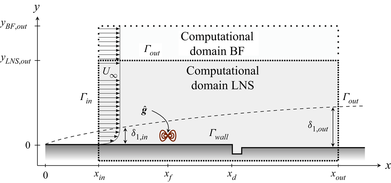
Figure 2. Sketch of the computational domain for the base flow (BF) and for the LNS computations.
A two-dimensional triangulation of the domain is performed with the FreeFem++ finite element library (Reference HechtHecht, 2012) with a Delaunay–Voronoi algorithm. Equations (2.3) are discretized with Taylor–Hood finite elements  $\mathcal {P}_2$ for the velocity field and $\mathcal {P}_1$ for the pressure. The nonlinear solution of the base flow is obtained with a classical Newton method, by progressively decreasing the value of the kinematic viscosity $\nu$ from $\nu = 1\,{\rm m}^2\,{\rm s}^{-1}$ until the value corresponding to the desired Reynolds number $ {\textit {Re}_{\delta _{1,{d}}}}$ is reached. Thus, the approximated solution at the $k$th iteration is obtained as follows:
 \begin{equation} \boldsymbol{Q}^k = \boldsymbol{Q}^{k-1} + \boldsymbol{\delta Q}^k. \end{equation}
Here,  $\boldsymbol {\delta Q}^k$ is the solution increment obtained by solving the linear problem
 \begin{equation} \boldsymbol{\mathsf{J}}\left(\boldsymbol{Q}^{k-1}\right) \boldsymbol{\delta Q}^k = {-}\boldsymbol{\mathsf{NS}}\left(\boldsymbol{Q}^{k-1}\right), \end{equation}
where  $\boldsymbol{\mathsf{NS}}$ and $\boldsymbol{\mathsf{J}}$ are, respectively, the Navier–Stokes operator and its Jacobian. The Newton algorithm solves the linear system (2.13) until $\left \lVert \boldsymbol{\mathsf{NS}}(\boldsymbol {Q}) \right \rVert _2<10^{-12}$.
2.3.3 The LNS computations
Once the base flow is calculated, the TS waves are artificially excited by introducing a volume force term  $\boldsymbol {g'} = (g_x',g_y')^{\rm T}$ into the LNS equations. This forcing is only prescribed on a tiny part of the computational domain and has a zero spatial distribution $\hat {\boldsymbol {g}}$ according to the $x$-direction: $\hat {\boldsymbol {g}}= (\hat {g}_x,\hat {g}_y)^{\rm T} = (0,10^{-5})^{\rm T}$. It extends in the longitudinal direction from an abscissa $ {x_{{f}}}$ to an abscissa $( {x_{{f}}}+0.002)$, and in the normal direction over a height $ \delta _{1,{in}}$. The abscissa $ {x_{{f}}}$ is chosen as the critical point delimiting the unstable domain of a Blasius boundary layer, i.e. at which $ {\textit {Re}_{\delta _{1}}}=520$, as shown in figure 3.

Figure 3. Neutral curve of a Blasius boundary layer obtained by LST and range of reduced frequencies calculated for the  $N$-factor envelope calculation.
The computational domain for the LNS calculations is similar to the base flow domain, but has a reduced height  $ {y_{{LNS},{out}}} = 15 \delta _{1,{out}}$ to avoid having too many vertices. The base flow is therefore interpolated onto the new mesh and equations (2.6) are discretized with Taylor–Hood finite elements $\mathcal {P}_2$ for the velocity field and $\mathcal {P}_1$ for the pressure. Whether for the base flow or the LNS computations, matrix inversion is performed by PETSc (Reference Balay, Abhyankar, Adams, Benson, Brown, Brune and ZhangBalay et al., 2021).
The LNS calculations are performed both on a smooth surface and on a surface with defect, for 91 non-dimensional reduced frequencies in the range  $F \in [25,160]$ to generate the $N$-factor envelope. This frequency region is represented in figure 3 and is chosen because it represents unstable frequencies which may undergo sufficient amplification to trigger the transition.
2.4 Code validation
2.4.1 Base flow
The base flow considered for validation is a boundary layer developing on a flat plate without surface imperfection or pressure gradient, with a Reynolds number based on the inlet displacement thickness  $ {\textit {Re}_{\delta _{1,{in}}}} = 371$. Non-dimensional velocity profiles are plotted at different boundary layer abscissae in figure 4(a) and show the self-similar feature of this flow. The black dashed curve corresponds to the theoretical profile obtained by solving the Blasius equation. The displacement thickness $\delta _1$ is plotted in figure 4(b) for several abscissae. One can observe that the results are very similar to the analytical solutions, indicating that the calculated boundary layer acts well as a Blasius boundary layer.

Figure 4. (a) Velocity profiles at different abscissae of the boundary layer and (b) evolution of the displacement thickness  $\delta _1$ in the boundary layer.
2.4.2 The LNS results
In order to validate the resolution of (2.6), the  $N$-factor envelope for the flat plate corresponding to the base flow of § 2.4.1 was calculated. The result is plotted in figure 5(a) and is compared with the amplification curve from a local stability calculation. The non-parallel effects taken into account by the LNS computation and ignored by LST have a slight stabilizing effect on the boundary layer, which may partly explain why the amplification of unstable waves starts for a higher Reynolds number in our case than in the local analysis. A second possible justification is that the very high frequencies are not calculated, as can be seen in figure 3. However, this does not affect the information about the transition position insofar as the slopes of the two envelope curves merge from a value of $N$ much lower than the traditional critical $ {N_{{tr}}}$-factor, once slightly lower frequencies are considered.

Figure 5. (a) The  $N$-factor envelope curve for a flat plate and (b) $N$-factor curves for the frequencies $f=300$ Hz (blue curve), $f=500$ Hz (red curve), $f=700$ Hz (green curve) and the envelope curve (black curve) for a boundary layer in the presence of a BFS.
To validate our method in the presence of surface imperfections, the configuration studied by Reference Hildebrand, Choudhari and ParedesHildebrand et al. (2020) is reproduced. The boundary layer encounters a BFS with slope  $\theta =75^{\circ }$ and height $h/ \delta _{1,{d}}=0.72$ at the abscissa $ {x_{{d}}} = 0.3\,{\rm m}$. The flow has the following characteristics: a displacement thickness $ \delta _{1,{d}} = 6.9\times 10^{-4}\,{\rm m}$ and a free-stream unit Reynolds number $ \textit {Re}_{\infty } = 1.86\times 10^6\,{\rm m}^{-1}$. Figure 5(b) compares the $N$-factor curves for different frequencies and the envelope curve obtained by our method with those obtained by Reference Hildebrand, Choudhari and ParedesHildebrand et al. (2020) and the results match perfectly, validating $\texttt{P}{\small {\texttt {IMS}}}\texttt{2D}$ in the presence of surface irregularities.
3. Study of a critical defect
A critical defect is studied in this section in order to detail the database generation process for a particular case. The defect configuration is such that  $h_1^\ast =1.72$, $h_2^\ast =0.47$, $b^\ast =7.54$ and $ {\textit {Re}_{\delta _{1,{d}}}}=1795$.
3.1 Base flow results
Boundary layer stability calculations require excellent accuracy in the base flow. The use of a finite element method allows the use of an unstructured mesh and local adaptations of the mesh. Thus, the initial mesh is automatically adapted to the solution  $\boldsymbol {Q}=(\boldsymbol {U},P)$ of the previous iteration when $ {\textit {Re}_{\delta _{1,{d}}}}>100$, and then adapted one last time after the final iteration thanks to the function adaptmesh of FreeFem++. This adaptation procedure is detailed in Reference HechtHecht (1998) and adapts the mesh to the Hessian matrix of the solution. As an example, initial and final adapted meshes are shown in figure 6.

Figure 6. (a) Initial and (b) final mesh after adaptation procedure. In both cases, a zoom is performed in the vicinity of the defect.
The non-dimensional streamwise velocity field exhibits a separation bubble behind the downward side of the gap, extending downstream of the defect. Figure 7(a) shows the displacement thickness  $\delta _1(x)$ and figure 7(b) the pressure distribution at the wall $P(x,y_{{wall}})$. The presence of the defect generates a favourable pressure gradient upstream of the gap, followed by a strong adverse pressure gradient region. Finally, there is a zone with a favourable pressure gradient approaching zero at the infinite downstream of the defect. These pressure variations explain the separation bubble and have an impact on the boundary layer thickness. The boundary layer becomes thinner just upstream of the gap when the pressure gradient is negative, and then thickens in the defect. At a certain distance from the gap, the boundary layer regains the behaviour of an unperturbed Blasius boundary layer.

Figure 7. (a) Boundary layer displacement thickness and (b) pressure distribution at the wall.
3.2 Instability analysis
3.2.1 Analysis of the envelope $N$-factor

Once the base flow is calculated, it is interpolated on the mesh used for the stability study. Equations (2.6) are solved for 91 non-dimensional reduced frequencies in the range  $F \in [25,160]$ and the TS wave amplification curves at the specified frequencies are obtained. The maximum of these amplifications gives the $N$-factor envelope in blue in figure 8. This curve is compared with the $ {N_{sm}}$ curve obtained for a smooth case and allows us to visualize quantitatively the effect of the gap on the TS wave amplification.

Figure 8. The  $N$-factor envelope curve with defect and for the same aerodynamic configuration but without defect. The figure also shows the amplification curves for all calculated frequencies (grey curves) as well as that of the most amplified frequency ( $F=58$).
At the upstream infinity, the amplification of the perturbations is equivalent with or without irregularity. Slightly upstream of the defect, the favourable pressure gradient region visible in figure 7(b) tends to stabilize the disturbances by thinning the boundary layer, and the  $N$-factor decreases slightly compared with the smooth case. However, just after the gap, the displacement thickness increases abruptly due to the strong positive pressure gradient and the boundary layer becomes much more unstable. This results in a very sharp local increase in the $N$-factor to a $ {N_{max}}$ value, due to the strong amplification of high frequency waves in the mixing layer forming downstream of the step in the detached region. Nevertheless, TS waves of these frequencies are rather stable for boundary layers and dissipate after the gap. The purple curve in figure 8 corresponds to the reduced frequency $F = 85$ and illustrates this phenomenon. The TS wave development corresponding to this frequency can be seen qualitatively in figure 9. On the other hand, TS waves of lower frequencies are also amplified by the defect but to a lesser extent, and the $N$-factor recovers the behaviour of the flat plate configuration at the downstream infinity but shifted by a $ \Delta N_{far}$ factor. This is illustrated by the orange curve corresponding to the reduced frequency $F = 25$.

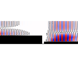
Figure 9. Real part of the streamwise velocity disturbance for a TS wave of reduced frequency  $F = 85$.
3.2.2 Calculation of the $ {\Delta N}$

Two  $ {\Delta N}$ arise from this analysis: a $ \Delta N_{max}$ corresponding to a local maximum of the $N$-factor located just after the gap, and a $ \Delta N_{far}$ at the downstream infinity. The calculation of $ \Delta N_{max}$ is straightforward since it corresponds to the maximum difference between the envelope curve of both the smooth and defect cases. In the following, the $ {N_{max}}$ is always defined as the value of the envelope $N$-factor of the defect case at the location of the $ \Delta N_{max}$. This value will not always correspond to the maximum value of the $N$-factor in the computational domain depending on the types of defects considered and the Reynolds number of the flow.
On the other hand, the determination of  $ \Delta N_{far}$ is more difficult because it is not constant but slightly decreasing with the distance to the defect, as shown in figure 10. In this paper, the $ \Delta N_{far}$ is defined as the first point for which the derivative $\mathrm {d}( {\Delta N})/\mathrm {d}x$ returns to a constant value. Determining $ \Delta N_{far}$ as soon as the effects of $ \Delta N_{max}$ are no longer felt in the flow allows us to obtain the most conservative value possible, which is of some use for an industrial application.

Figure 10. Evolution of  $ {\Delta N}$ and its first derivative.
As an example, the transition  $N$-factor of the present case is chosen at $ {N_{{tr}}}=7$ and is representative of a wind tunnel experiment for a TS wave transition scenario. The case considered here is thus critical insofar as it triggers transition at $(x- {x_{{d}}}) = 25\, \delta _{1,{d}}$, immediately downstream of the defect due to the $ \Delta N_{max}$ effect, while the transition is triggered for the smooth case for $(x- {x_{{d}}}) = 647\, \delta _{1,{d}}$. The TS wave responsible for triggering the transition has a reduced frequency $F=58$ and corresponds to the green curve in figure 8.
3.2.3 Comparison with the literature
The  $ {\Delta N}$ obtained from experimental measurements is defined as the difference between the value of the transitional $N$-factor of the smooth case and the value of the envelope curve at the transition abscissa in the presence of a defect. We will then refer to it as $ {\Delta N}_{{Exp}}$. On the other hand, the inconvenience of numerical results from LST, PSE or LNS calculations as in this paper is that the transition position is not known, which prevents a similar definition of the $ {\Delta N}$ responsible for the transition. Thus, $ {\Delta N}(x)$ is computed as the difference between the two envelope curves (with and without defect) in the entire computational domain without considering an actual transition location. This difference in definition between numerical and experimental $ {\Delta N}$ has already been raised by Reference Crouch and KosoryginCrouch and Kosorygin (2020). These authors instead mention a ${\rm \Delta} n$ for numerical studies which, unlike the experimental $ {\Delta N}_{{Exp}}$, is not specifically related to the perturbations whose frequencies are responsible for the transition but is seen rather as a local amplification factor. The comparison between numerical and experimental results is therefore tricky.
3.2.4 Distortion of TS waves by the defect
In order to visualize the evolution of the most unstable wave in the flow, dimensionless profiles of the amplitude functions  $(\hat {u},\hat {v},\hat {p})$ are plotted for different abscissae in figure 11, where $x^\ast = (x- {x_{{d}}}) / \delta _{1,{d}}$. Upstream of the defect ( $x^\ast = -5$), the perturbation profiles correspond to those of a TS wave, with the presence of a main peak of $\hat {u}$ close to the wall, followed by a local minimum at the maximum location of $\hat {v}$. When crossing the gap ( $x^\ast = 10$), the profiles are distorted and $\hat {u}$ has two main peaks. The destabilization mechanism then changes from a viscous instability to a combination of viscous and Kelvin–Helmholtz (KH) instability. Close to the defect, the higher peak ${\tiny {\bigcirc{\kern-4pt 2}}}$ in the flow has a larger amplitude than the peak ${\tiny {\bigcirc{\kern-4pt 1}}}$ situated closer to the wall, but this tendency is inverted away from the defect ( $x^\ast = 30$) and the viscous instability becomes predominant again. Finally, the ${\tiny {\bigcirc{\kern-4pt 2}}}$ peak disappears and profiles characteristic of a TS wave are observed again ( $x^\ast = 100$).

Figure 11. Scaled profiles of the disturbance at frequency  $F=58$ at different abscissae: (a) $x^\ast = -5$; (b) $x^\ast = 10$; (c) $x^\ast = 30$; and (d) $x^\ast = 100$.
The presence of these two peaks is visible in the  $\hat {u}$ field plotted in figure 12 near the gap. The orange region above the first edge for $x^\ast <0$ corresponds to the main peak of the TS wave in figure 11(a). After the defect, this area is extended in the groove alignment while increasing in amplitude and corresponds to the peak ${\tiny {\bigcirc{\kern-4pt 2}}}$, while a second region of progressive amplification appears in the near wall corresponding to the peak ${\tiny {\bigcirc{\kern-4pt 1}}}$. When moving away from the defect, these two amplification regions merge to form a single one, typical of TS waves.

Figure 12. Streamwise velocity disturbance for a TS wave of reduced frequency for  $F = 58$ (zoom near the defect).
Both viscous and KH instabilities indicate that the mechanisms responsible for the destabilization of the boundary layer are more complicated than a simple over-amplification of TS waves. At first sight, it would be necessary to filter out the contribution of TS waves alone in order to use the  $ {\Delta N}$ method in this region of the flow to properly separate the contribution of the two unstable modes. However, $ {N_{max}}$ is reached in figure 8 at the abscissa $x^\ast = 100$, which corresponds to the TS profiles shown in figure 11(d). At this x-value, both modes have combined into a single one, and the KH instability does not seem to be responsible for the $ \Delta N_{max}$. In the rest of the paper, only TS wave transition scenario will be considered.
4. Neural network model
4.1 Definition
An artificial neuron is a nonlinear function that associates an input vector  $\boldsymbol{\mathsf{x}} = (\boldsymbol{\mathsf {x}}_1, \ldots,\boldsymbol{\mathsf {x}}_{\boldsymbol{\mathsf {n}}})$ with an output $\boldsymbol{\mathsf {y}}$, as follows:
 \begin{equation} \boldsymbol{\mathsf{y}} = \sigma\left(\sum_{i = 1}^{\boldsymbol{\mathsf{n}}}{\boldsymbol{\mathsf{w}}_i\boldsymbol{\mathsf{x}}_i} + \boldsymbol{\mathsf{b}}_i\right), \end{equation}
where  $\sigma$ is an activation function, $\boldsymbol{\mathsf{w}} = (\boldsymbol{\mathsf {w}}_1, \ldots,\boldsymbol{\mathsf {w}}_{\boldsymbol{\mathsf {n}}})$ is the vector of connection weights and $\boldsymbol{\mathsf {b}}$ is a bias. The activation function introduces a nonlinearity, allowing the neuron to represent arbitrarily complex functional relations between input variables.
A NN is a structure composed of successive hidden layers between the input layer and the output layer, where the output of a neuron becomes the input of all the units in the next layer. The learning process then consists of iteratively adjusting the weights and biases of the network by minimizing a loss function  $\mathcal {L}$.
4.2 Generation of training data
The inputs of the NN are  $ {\textit {Re}_{\delta _{1,{d}}}}$ as the aerodynamic variable and $h_1^\ast$, $h_2^\ast$ and $b^\ast$ as geometric parameters. Geometric ranges of input parameters have been selected to represent both stable and critical cases that could trigger the transition, according to the criteria defined by Reference Beguet, Perraud, Forte and BrazierBeguet, Perraud, Forte, and Brazier (2017). Discretization of the input parameter domain was performed by Latin-hypercube sampling with 750 samples. This method, described by Reference McKay, Beckman and ConoverMcKay, Beckman, and Conover (1979), positions each sample according to the location of previously positioned specimens, to ensure that they do not have common coordinates. This scheme has the advantage of not requiring more samples to cover more dimensions.
During sampling, the region covered by  $h_2^\ast$ is discretized so that we always have $0 < h_2^\ast / h_1^\ast < 1$. This choice is made in order to treat here only cases of step and gap defects with a ‘descending’ trend, i.e. with the second edge smaller than the first. For each sample of input parameters generated, $\texttt{P}{\small {\texttt {IMS}}}\texttt{2D}$ provides as output the values $ \Delta N_{max}$ and $ \Delta N_{far}$, which will be the outputs to be predicted by the NN, as illustrated in figure 13. The distribution of the input parameters is shown in figure 14. More specifically, the range of Reynolds number $ {\textit {Re}_{\delta _{1,{d}}}}$ considered extents over $[901.5; 1999.4]$, the height $h_1^\ast$ over $[0.1; 2.99]$ , the height $h_2^\ast$ over $[0.004; 2.9]$ and the width over $[0.5; 14.9]$.

Figure 13. Database creation methodology.

Figure 14. Input parameter distribution of the NN: (a) heights, (b) width and (c) Reynolds number.
All the cases used to supply the database and which have been calculated by  $\texttt{P}{\small {\texttt {IMS}}}\texttt{2D}$ are subcritical with respect to the bypass transition. More concretely, the calculation of the stationary base flow cannot converge if the flow presents a global instability. According to Reference Alam and SandhamAlam and Sandham (2000), when the adverse velocity magnitude in the recirculation zone exceeds 15 %–20 % of the upstream infinite velocity, the flow can become globally unstable. This is what seems to happen in our cases when $h_1^\ast >3$, so only defects with $h_1^\ast <3$ have been considered.
4.3 Database analysis
Figure 15 illustrates the influence of the input geometrical parameters on the different  $ {\Delta N}$ for each case in the database. Analysis of figure 15(a) shows firstly that the $ \Delta N_{max}$ is more important when the height $h_1^\ast$ is high. Moreover, the $ \Delta N_{max}$ is lower when the height $h_2^\ast$ is higher, i.e. a defect close to a BFS is more destabilizing than a cavity type defect.

Figure 15. (a,b) Evolution of  $ \Delta N_{max}$ as a function of geometric parameters and (c) evolution of $ \Delta N_{max}$ as a function of $ \Delta N_{far}$.
As shown in figure 15(b), the highest values of  $ \Delta N_{max}$ correspond to the highest $b^\ast$ when ${\rm \Delta} h = |h_1^\ast - h_2^\ast | < 0.5$. On the other hand, beyond this threshold, the width does not seem to play a determining role and a correlation seems to exist between the heights difference ${\rm \Delta} h$ and the $ \Delta N_{max}$ value. Moreover, the $ \Delta N_{max}$ seems to reach a limit around 2 for ${\rm \Delta} h < 0.5$, i.e. for gaps with relatively similar heights, while a behaviour closer to the BFS one becomes more destabilizing when ${\rm \Delta} h$ increases. Similar results were shown by Reference Crouch, Kosorygin, Sutanto and MillerCrouch et al. (2022) in their model indicating that the gap acts as a BFS for a shallow gap, but that the width becomes dominant for deep gaps.
There also appears to be a strong linear relation between the  $ \Delta N_{max}$ and $ \Delta N_{far}$ values, as shown in figure 15(c). This could translate in future studies into the need to know only one of the two $ {\Delta N}$ to predict the other.
4.4 Neural network predictions and validation
An attempt by the authors to predict  $ \Delta N_{far}$ and $ \Delta N_{max}$ by linear techniques was not conclusive, so the use of nonlinear models with NNs is preferred. The model is available on zenodo at https://doi.org/10.5281/zenodo.7101195.
4.4.1 Implemented NNs
Given the relatively small number of samples in the database, the NNs used in this work have a rather simple architecture. Neural networks with different structures regarding the number of hidden layers and the number of neurons in each layer are considered. The structure of these networks is detailed in table 1. Each of these models is based on a rectified linear unit activation function and an Adam optimizer. Adam optimization is a stochastic gradient descent method used to minimize the cost function. Each training of the network is performed on a normalized training dataset representing 80 % of the total dataset (i.e. 600 samples) and randomly selected, while the validation is done on the remaining 20 % which have never been seen by the network (i.e. 150 samples).
Table 1. Details of networks architectures and results. Architecture of the network corresponds to the number of neurons in each layer.

We consider a learning base  $(\boldsymbol{\mathsf {x}}_1^{(i)},\ldots,\boldsymbol{\mathsf {x}}_{\boldsymbol{\mathsf {k}}}^{(i)},\boldsymbol{\mathsf {y}}^{(i)})$ with $\boldsymbol{\mathsf {n}}$ observations, where $\boldsymbol{\mathsf{x}}^{(i)}$ are the input variables of the $i$th observation and $\boldsymbol{\mathsf {y}}^{(i)}$ is the variable to be predicted. The loss function to be minimized by the network during training is defined as the mean square error between the real values $\boldsymbol{\mathsf {y}}^{(i)}$ and the values predicted by the NN $\tilde {\boldsymbol{\mathsf {y}}}^{(i)}$
 \begin{equation} \mathcal{L} = \frac{1}{\boldsymbol{\mathsf{n}}}\sum_{i = 1}^{\boldsymbol{\mathsf{n}}} (\tilde{\boldsymbol{\mathsf{y}}}^{(i)}-\boldsymbol{\mathsf{y}}^{(i)})^2. \end{equation}
The evolution of the loss function during the training process is plotted in figure 16 as a function of the number of epochs, i.e. the number of times that the network sees the training dataset entirely and adapts its weights and biases. An early stopping criterion is used to limit overfitting, stopping the training when the validation error no longer improved. Thus, a learning loop will check at the end of each epoch if the loss function has not decreased over the last five epochs. The learning of the network is completed when the decrease stops.

Figure 16. Evolution of the loss function  $\mathcal {L}$ according to the number of epochs of the training process.
When the model is trained several times, the results may be slightly different. A  $K$-fold cross-validation is therefore used to get an indication of the model performance. The database is divided into five groups from which one sample is chosen as the validation set while the other four constitute the training set. After training, a validation performance criterion is obtained. This operation is repeated by selecting another validation sample among the predefined blocks, and at the end of the procedure five performance scores are obtained, one per fold. The metric used to quantify the accuracy of the models is the mean absolute error (MAE) $\epsilon _{{MAE}}$ described as
 \begin{equation} \epsilon_{{MAE}} = \frac{1}{m}\sum_{i = 1}^m{\left|\boldsymbol{\mathsf{y}}^{(i)}-\tilde{\boldsymbol{\mathsf{y}}}^{(i)}\right|}, \end{equation}
with  $m$ being the size of the validation dataset. Mean and standard deviation of the five MAE scores are listed in table 1 for each network.
4.4.2 Validation of NN results
Once validated, the NN model predictions are compared with the experimental results of Reference Methel, Forte, Vermeersch and CasalisMethel, Forte, Vermeersch, and Casalis (2021). These authors have investigated experimentally the effect of gaps in transition on a flat plate with wall suction. Some cases without suction were extracted to be compared with the  $ \Delta N_{far}$ predictions from the NN. This comparison can be found in table 2. Taking into account the value of $ \Delta N_{far}$ rather than $ \Delta N_{max}$ is justified in figure 18 insofar as the experimental transition point is located far enough from the defect that the effects due to $ \Delta N_{max}$ are no longer apparent. This figure will be analysed in more detail in § 5. Note that all these geometrical configurations are out of the learning zone, since the networks have never studied defects for which $h_1^\ast =h_2^\ast$. Moreover, the last two gaps are also out of the learning zone in terms of widths. This may have an effect on the performance of the models. Nevertheless, the orders of magnitude of the predictions are respected and the agreement between the ${\rm \Delta} N_{{Exp}}$ obtained experimentally and the $ \Delta N_{far}$ predicted is good considering the $\epsilon _{{MAE}}$ value of each NN.
Table 2. Comparison between the Reference Methel, Forte, Vermeersch and CasalisMethel et al. (2021) experimental results on a gap and the  $ \Delta N_{far}$ predicted by the NN.

In order to verify the network's ability to correctly predict the  $ {\Delta N}$ outside of its training area, the Reference Wang and GasterWang and Gaster (2005) experimental results for BFSs were reproduced. The parameter $h_2^\ast$ is set to zero, while the parameter $b^\ast$ is set to zero in a first step and set to 20 in a second step, to approximate as closely as possible the geometry of a BFS. A case with $b^\ast =0$ is geometrically close to a BFS, while the $b^\ast =20$ case allows us to perceive the effect of a large width associated with a zero height $h_2^\ast$ on the behaviour of the NN. This configuration does not make sense from a physical point of view. Both cases are situated outside the learning area of the networks. Neural predictions are also compared with the following correlations from Reference Hildebrand, Choudhari and ParedesHildebrand et al. (2020):
 \begin{equation} {\rm \Delta} N_{Wang} =
\begin{cases} 0 & \text{if } h^\ast< 0.35, \\ 4 h^\ast-
1.4 & \text{if } h^\ast\geq 0.35, \end{cases}
\end{equation}
\begin{equation} {\rm \Delta} N_{Wang} =
\begin{cases} 0 & \text{if } h^\ast< 0.35, \\ 4 h^\ast-
1.4 & \text{if } h^\ast\geq 0.35, \end{cases}
\end{equation}
and
 \begin{equation} {\rm \Delta} N_{Hild} =
\begin{cases} 2.47 {h^\ast}^2 + 0.62 h^\ast & \text{if }
h^\ast< 0.38, \\ 3 h^\ast- 0.55 & \text{if }
h^\ast\geq 0.38. \end{cases}
\end{equation}
\begin{equation} {\rm \Delta} N_{Hild} =
\begin{cases} 2.47 {h^\ast}^2 + 0.62 h^\ast & \text{if }
h^\ast< 0.38, \\ 3 h^\ast- 0.55 & \text{if }
h^\ast\geq 0.38. \end{cases}
\end{equation}
Note that the  ${\rm \Delta} N_{Wang}$ correlation is a linear relation extrapolated by Reference Hildebrand, Choudhari and ParedesHildebrand et al. (2020) from the experimental data of Reference Wang and GasterWang and Gaster (2005) using a least squares method. As indicated by Reference Hildebrand, Choudhari and ParedesHildebrand et al. (2020), the numerical results leading to correlation (4.5) as well as Wang's experimental points correspond to cases for which the transition position is located far enough downstream of the defect so that the transition is not related to the $N$-factor overshoot ( $ \Delta N_{max}$ in this paper). The comparison of the neural results with the literature is therefore made with the predictions of $ \Delta N_{far}$. Results from network $\mathbb {B}$ are plotted in figure 17 and show reasonable agreement between the experiment and the neural predictions, keeping in mind that the network has not been trained with a pure BFS configuration. Considering that Reference Wang and GasterWang and Gaster (2005) assume the uncertainty on the transition position uncertainty to be approximately ${\pm }5\,{\rm mm}$ in a flat plate configuration, the uncertainty on the experimental ${\rm \Delta} N$ can fairly be considered to be around ${\pm }0.1$. The observed differences between both $b^\ast =0$ and $b^\ast =20$ cases are almost invisible and suggest that the network behaves identically regardless of the width when $h_2^\ast = 0$. The NN results corresponding to $ {\textit {Re}_{\delta _{1,{d}}}} > 2000$, located outside the training region for the Reynolds number, are represented by filled symbols to differentiate them and have a larger error compared with the experimental results. Moreover, for $h_1^\ast > 1.2$, our results are located between the curves corresponding to correlations (4.4) and (4.5). Finally, the neural results corresponding to the cases $h_1^\ast <0.9$ and $h_1^\ast >1.7$ have been obtained by considering an arbitrary $ {\textit {Re}_{\delta _{1,{d}}}}=1600$ and are only compared with the correlations. These cases show an excellent agreement with the relation of Reference Hildebrand, Choudhari and ParedesHildebrand et al. (2020), and prove again the robustness of NN models for defect cases outside the training range.

Figure 17. Comparison between predictions of network  $\mathbb {B}$, wind tunnel experiments of Reference Wang and GasterWang and Gaster (2005) and empirical correlations for BFSs. The filled symbols correspond to ranges of $ {\textit {Re}_{\delta _{1,{d}}}}$ for which the network has not been trained.
5. Discussion on the use of NN
Developed neural models for  ${\rm \Delta} N$ prediction are restricted to two-dimensional and incompressible flows. However, they represent a first step towards the modelling of surface defects’ influence on transition in flight conditions. Their range of use for each of the input parameters is summarized in table 3.
Table 3. Range of input parameters (in absolute value) for which the NNs  $\mathbb {A}$, $\mathbb {B}$ and $\mathbb {C}$ were trained.

The use of neural models implies that the user must dispose of the envelope curve of the  $N$-factor corresponding to the smooth case. This curve is usually obtained by an LST calculation. Guidelines are provided on how to use the NN, as illustrated by figure 18. The defect considered is a gap of heights $h_1^\ast =h_2^\ast =1.9$, width $b^\ast =12.7$ and located at $ {\textit {Re}_{\delta _{1,{d}}}}=1640$. Experimental results from Reference Methel, Forte, Vermeersch and CasalisMethel et al. (2021) yield $ {N_{{tr}}}=6.2$. In a first step, the user can check if the transition $ {N_{{tr}}}$ is reached thanks to the effect of the $ {N_{max}}$ by adding the $ \Delta N_{max}$ predicted by the NN to the smooth case $N$-factor at the location of the surface irregularity, or immediately downstream of the defect in a limit $0 \leq (x- {x_{{d}}}) < 100\, \delta _{1,{d}}$. This limit remains arbitrary but allows us to stay in a region where the $ {N_{max}}$ effects are noticeable according to the study of the database by the authors. The addition of the $ \Delta N_{max}$ corresponds to the purple curve in figure 18 and in this case, the $N$-factor remains smaller than $ {N_{{tr}}}$. In a more general case, if the $ \Delta N_{max}$ is not sufficient to exceed $ {N_{{tr}}}$, the user can then use the prediction of $ \Delta N_{far}$ to get an indication of the defect influence. Since $ \Delta N_{far}$ is extracted by $\texttt{P}{\small {\texttt {IMS}}}\texttt{2D}$ quite early in the flow, once $\mathrm {d} {\Delta N}/\mathrm {d}x$ becomes constant after the $ \Delta N_{max}$ effects have dissipated, the predicted value is rather conservative. Addition of the smooth case and the neural prediction of $ \Delta N_{far}$ corresponds to the green curve in figure 18. The difference in transition position ${\rm \Delta} x_{{tr}}$ between the LNS calculations and the neural results is approximately $11 \delta _{1,{d}}$, i.e. in this case ${\rm \Delta} x_{{tr,LNS}}\simeq 0.0012$ m. In order to properly illustrate this example, the addition of the experimental $ {\Delta N}$ to the smooth case corresponds to the orange curve. The difference between the experimental and NN-predicted transition position is approximately $63 \delta _{1,{d}}$, i.e. ${\rm \Delta} x_{{tr,Exp}}\simeq 0.0073$ m.

Figure 18. Comparison between the envelope curve obtained by LNS and by the predictions of the NN  $\mathbb {B}$ for the second case of table 2.
For comparison, the computational time to obtain a prediction from the NN is 0.2 s, while the computation of the  $N$-factor envelope curve by $\texttt{P}{\small {\texttt {IMS}}}\texttt{2D}$ of the second case in table 2 required 12 576 s (739 s for the base flow and 11 837 s for the LNS computation of the 91 reduced frequencies). Note that the LNS computation time can, however, be reduced by considering fewer frequencies but losing accuracy. For information, the time required to train the three networks was 39 s with an Intel(R) Xeon(R) Gold 6130 CPU @ 2.10 GHz. The difference in computational time between using NN and numerical resolution by stability analysis is therefore clearly and significantly in favour of the models.
Nevertheless, the method of predicting the different  $ {\Delta N}$ presented in this work has some limitations. The first important remark is that the predictions from the NN are only valid for a TS wave induced transition. Potential global instabilities that can occur for specific geometries have not been studied in this paper. It should be noted that the presence of global instability mechanisms prevents the resolution of the base flow by $\texttt{P}{\small {\texttt {IMS}}}\texttt{2D}$ since no stationary solution exists. The transition processes considered here will therefore only involve natural transition paths, i.e. for which the transition is due to the exponential growth of TS waves by modal amplification.
Secondly, the neural models are limited to a certain range of parameters corresponding to those for which the NNs have been trained. The robustness of the results outside the training range is not guaranteed. Besides, the same problem exists for the empirical correlations which are only valid within the range of experimentally studied parameters. However, the predictions corresponding to the BFS and presented in figure 17 seem to indicate that the networks do not make erroneous predictions as long as the physical mechanisms involved in the transition process remain the same, although there is a slightly larger difference between the neural predictions and the experimental  $ {\Delta N}$ when $ {\textit {Re}_{\delta _{1,{d}}}}$ is out of the learning zone.
Finally, it has been shown by Reference Hildebrand, Choudhari and ParedesHildebrand et al. (2020) that the location of the transition position could not always be deduced from the knowledge of the values of  $ \Delta N_{max}$ and $ \Delta N_{far}$. There are two instances of BFSs in this paper ( $h_1^\ast =1.12$ and $h_1^\ast =1.6$) for which the transition position does not correspond to the abscissa at which the envelope $N$-factor reaches the $ {N_{{tr}}}$ value, but rather seems to result from a different physical mechanism. Furthermore, the LNS calculations do not allow the determination of a transition position that could have provided the value of the transition $ {\Delta N}$. The proposed method is therefore only a first approach to the problem considered and various improvements can be made to enhance the accuracy of the models.
6. Conclusion
A new method for predicting the transition to turbulence of incompressible two-dimensional boundary layers in the presence of gap-shaped surface defects has been presented. This method is based on the  $ {\operatorname {e}^{N}}$ method and a NN is used to determine the values of the $ \Delta N_{max}$ and $ \Delta N_{far}$ generated by the surface irregularity when the transition is driven by a natural transition scenario induced by TS wave amplification. The proposed model relies on four distinct parameters defining the geometry of the defect and its aerodynamic environment, which are its two heights $h_1$ and $h_2$, its width $b$ and the Reynolds number based on the displacement thickness of a Blasius boundary layer at the defect position $ {\textit {Re}_{\delta _{1,{d}}}}$.
A database of 750 surface defects was generated with the  $\texttt{P}{\small {\texttt {IMS}}}\texttt{2D}$ code whose advantage is that it is quite flexible in the creation of the mesh, allowing us to easily implement boundary layer stability calculations, while the currently existing methods for the transition prediction in the presence of defects are rather complex to implement. This code has been validated in the case of a flat plate and around a BFS, showing good agreement with results from LST or AHLNS calculations.
Three NNs of different architectures have been developed and trained to predict  $ \Delta N_{max}$ and $ \Delta N_{far}$ using this database. The models have been trained for incompressible flows without a pressure gradient, for Reynolds numbers $ {\textit {Re}_{\delta _{1,{d}}}}\in [900\unicode{x2013}2000]$ and step-and-gap defects of dimensions $h_1^\ast \in [0.1\unicode{x2013}3]$, $h_2^\ast \in [0\unicode{x2013}3]$ and $b^\ast \in [0.5\unicode{x2013}15]$. The average error of the model is around $5\times 10^{-2}$ on either $ {\Delta N}$, which provides a fairly robust prediction of the criticality of the surface irregularity. Contrary to the empirical correlations existing in the literature, the model generated by the network generalizes to any type of gap as long as the characteristics of the defect are within the range of parameters studied by the network. The parametrization of the surface defects allows the model to be extended to other defects, for example for BFSs, by setting the parameters $h_2^\ast$ and $b^\ast$ to zero. Encouraging results have been presented in this sense.
In future work, some limitations must be overcome to further improve the efficiency of transition prediction by NNs. The first improvement would be to extend the operating range of the networks by considering larger gap widths and a wider range of Reynolds numbers. This would allow the models to increase their range of use, with a better consideration of real flight conditions, especially with respect to Reynolds number. In addition, the models could be improved by also considering defects such as FFSs and bumps, whose parametric representation would be similar to the gaps and BFSs studied here. Two input parameters could also be added to the models for a better representation of the real flight conditions. First, stability calculations in a compressible regime (subsonic and/or transonic) could be implemented to take into account the influence of the Mach number on the stability of the boundary layer. Moreover, the influence of a pressure gradient could also be taken into account in the models for a better representation of the NLF wing profiles. Finally, a last natural extension of the code, and thus of the neural models, would be the resolution of three-dimensional boundary layers to be able to simulate real surface defects and thus understand the influence of the latter on the development of cross-flow instabilities. Despite their rather simple architecture, the NNs used here produced good results, given the size of our dataset (750 samples). In order to handle larger volumes of data, it may be necessary to move on to more advanced architectures such as convolutional NNs (see for example Reference Guastoni, Güemes, Ianiro, Discetti, Schlatter, Azizpour and VinuesaGuastoni et al., 2021).
Supplementary material
The three NNs developed in this study are available at the following address: https://doi.org/10.5281/zenodo.7101195 (Reference Rouviere, Pascal, Méry, Simon and GrattonRouviere, Pascal, Méry, Simon, & Gratton, 2022). The repository also includes a Python script named Main.py and a Jupyter script named Main.ipynb that provide detailed explanations and examples on how to use these NNs. Further details on underlying data are available from the corresponding author (F.M.).
Funding statement
This work has been partly funded within the frame of the Joint Technology Initiative JTI Clean Sky 2, AIRFRAME Integrated Technology Demonstrator platform ‘AIRFRAME ITD’ (contract CSJU-CS2-GAM-AIR-2020-945521) being part of the Horizon 2020 research and Innovation framework programme of the European Commission.
Declaration of interests
The authors declare no conflict of interest.
Author contributions
A.R., F.M. and L.P. were involved with the fluid mechanics part, while A.R., S.G. and E.S. worked on the development of NNs.


 Open access