


Impact Statement
The staggered wavy-wall turbulence can represent the momentum transport over a natural dune (riverbed) formed through the interaction between turbulent momentum and sediment transports. The naturally formed dunes (riverbeds) are usually three-dimensional and large-scale topographies. Hence, the momentum transport over these kinds of dunes (riverbeds) is quite crucial in understanding the dynamics of geomorphology. The flow phenomenon is quite complex above this kind of terrain, such as the secondary flows. Secondary flow is known to appear in curved channel flow, the turbulent boundary layer and spanwise-heterogeneous wall turbulence, which is highly critical to modulation of the momentum transfer. Nevertheless, the generation of secondary flows and streamwise vortices still needs to be revealed in three-dimensional staggered wavy wall turbulence. Therefore, this study conducts numerical simulations of three-dimensional staggered wavy-wall turbulence and analyses the formation of secondary flows and streamwise vortices, which provides insight into our understanding of terrain-induced complex flow and effective ways to control the aeolian sand (sediment) transport.
1. Introduction
Aeolian sand (sediment) transportation can be easily found above a dune (riverbed) in nature, which is crucial in geomorphology formation and evolution. It is well known that the bed feature is determined by the flow regime (Reference RaudkiviRaudkivi, 1998). Generally, the beds can be classified as ripples and dunes. The dunes, formed in unidirectional flow, feature an approximate wavy pattern. Whereas the ripples, usually formed in oscillatory flow such as wave motion, feature irregular patterns. Reference AllenAllen (1968) concluded that a varied velocity is key to forming sinuous ripples. These ripples can develop into three-dimensional structures by the complex flow conditions, and are known as the linguoid or tetrahedral ripples. As there is an increase of the flow velocity, a transition from ripples into dunes can be found. The dunes, as a large-scale topography, can be divided into two-dimensional and three-dimensional shapes (Reference Omidyeganeh and PiomelliOmidyeganeh & Piomelli, 2013). The two-dimensional wavy-like dunes feature regularly characteristic wavelength and height. Whereas the irregular crestlines can be observed for a three-dimensional dune (Reference AshleyAshley, 1990). More specifically, sediment accumulation results in a staggered bump–concavity structure, which can be found in the process of dune evolution. According to the summary of the geometry of fluvial channels by Reference RaudkiviRaudkivi (1998), the beds can be simplified as three-dimensional wavy walls (Reference Zedler and StreetZedler & Street, 2001), which is achieved by superimposing a sinusoidal variation on the wavy wall along the spanwise direction. This simplification makes the comparison of flow over two-dimensional and three-dimensional dunes easier. For flow over two-dimensional dunes, there are commons that the flow separation and reattachment induced flow deceleration and acceleration, which are approximately unaffected by the dune shapes and Reynolds numbers (Reference Venditti and BauerVenditti & Bauer, 2005). However, a three-dimensional dune leads to a complex flow structure such as secondary flow (Reference Wang and ChengWang & Cheng, 2006). Therefore, as a more complex wall structure, a deeper insight into turbulent flow, especially the secondary flow, over three-dimensional dunes should be revealed.
The secondary flow usually appears in curved channel flows, turbulent boundary layer flows and spanwise-heterogeneous wall turbulence (Reference Medjoun, Vanderwel and GanapathisubramaniMedjoun, Vanderwel, & Ganapathisubramani, 2018; Reference NikuradseNikuradse, 1930; Reference PrandtlPrandtl, 1952; Reference Wang and ChengWang & Cheng, 2006; Reference Yang and AndersonYang & Anderson, 2017). Generally, the spanwise-heterogeneous wall is made up of a flat wall mounted with rough elements. These elements usually feature rectangular (Reference Medjoun, Vanderwel and GanapathisubramaniMedjoun et al., 2018) and triangular (Reference Zampiron, Cameron and NikoraZampiron, Cameron, & Nikora, 2020) cross-sections. Another spanwise-heterogeneous wall is built by imposing a spanwise sinusoidal elevation variance (Reference Wang and ChengWang & Cheng, 2006; Reference Zhang, Wang and LiuZhang, Wang, & Liu, 2021) based on the flat wall. There are common factors for turbulent flow over these different walls such as that the secondary flow is similar in directionality: the flow is transferred from the high-shear-stress region into the low-shear-stress region (Reference HinzeHinze, 1973; Reference Nugroho, Hutchins and MontyNugroho, Hutchins, & Monty, 2013; Reference Willingham, Anderson, Christensen and BarrosWillingham, Anderson, Christensen, & Barros, 2014). However, the strength of the secondary flow depends on the scale of the spanwise heterogeneity. As noted by Reference Vanderwel and GanapathisubramaniVanderwel and Ganapathisubramani (2015), the large-scale secondary flows are accentuated when the spacing of the roughness elements (the length of spanwise heterogeneity) is approximately proportional to the boundary layer thickness. According to the macro-feature of the secondary flows, Reference Yang and AndersonYang and Anderson (2017) suggested that there are three regimes according to the ratio of the length of spanwise heterogeneity (S) to the boundary layer thickness ( $\delta$), that is, the homogeneous roughness regime ( ${S}/{\delta }\le 0.2$), topography regime ( ${S}/{\delta }\ge 2$) and intermediate regime ( $0.2\le {S}/{\delta }\le 2$). There have been a large number of investigations of spanwise-heterogeneous wall turbulence for the homogeneous roughness and intermediate regimes (Reference Anderson, Barros, Christensen and AwasthiAnderson, Barros, Christensen, & Awasthi, 2015; Reference Castro, Kim, Stroh and LimCastro, Kim, Stroh, & Lim, 2021; Reference Hwang and LeeHwang & Lee, 2018; Reference Medjoun, Vanderwel and GanapathisubramaniMedjoun, Vanderwel, & Ganapathisubramani, 2020; Reference Mejia-Alvarez and ChristensenMejia-Alvarez & Christensen, 2013; Reference Stroh, Schäfer, Frohnapfel and ForooghiStroh, Schäfer, Frohnapfel, & Forooghi, 2020). The wall boundary under a homogeneous roughness regime can be considered roughness which only affects the near-wall momentum transport while not affecting the turbulent feature in the outer region (Reference Wangsawijaya, Baidya, Chung, Marusic and HutchinsWangsawijaya, Baidya, Chung, Marusic, & Hutchins, 2020), indicating outer region similarity (Reference Raupach, Antonia and RajagopalanRaupach, Antonia, & Rajagopalan, 1991; Reference TownsendTownsend, 1976). However, the naturally formed dunes (riverbeds) are not only spanwise heterogeneous but are also streamwise heterogeneous (or staggered heterogeneous). How a staggered heterogeneous wall affects secondary flow is not fully understood.
The three-dimensional wavy wall represents the natural dunes to some extent. The vortices induced by these bounded walls have attracted much attention. Studies pointed out that the three-dimensional wavy wall disrupts the large-scale coherent structures (Reference Ma, Xu, Sung and HuangMa, Xu, Sung, & Huang, 2020), generating vortices (Reference Zhang, Wang and LiuZhang et al., 2021), thus leading to momentum variation in the near-wall region. The main vortex structures include streamwise and spanwise vortices, with the latter produced via shear instability (Reference Omidyeganeh and PiomelliOmidyeganeh & Piomelli, 2011). Reference Bhaganagar and HsuBhaganagar and Hsu (2009) numerically investigated the turbulent flow over three-dimensional ripples, suggesting that there is irregular spanwise vorticity above the crest. However, affected by the turbulence, the streamwise and vertical vorticities show a dominant, organized and alternating pattern near the ripple. The effect of a three-dimensional wavy wall on vorticity was further verified in the experimental study by Reference Hamed, Kamdar, Castillo and ChamorroHamed, Kamdar, Castillo, and Chamorro (2015), who found the spanwise-heterogeneous wavy wall could limit the dynamics of spanwise turbulent vortical structures. Additionally, Reference Marchis, Milici and NapoliMarchis, Milici, and Napoli (2015) reported that the vortical structures of elongated shapes with a typical meandering behaviour are preserved in three-dimensional rough wall turbulence. This results in the abrupt reduction of both low- and high-momentum regions’ length in the streamwise direction while enlarging the streaks in the spanwise direction. The streamwise vortices change the temporal turbulent event, such as the vortex pairs, via upwash motion ejecting the near-wall low-momentum fluid into the upper average flow, modulating the momentum transport (Reference Yang and ShenYang & Shen, 2009). These studies suggest that the streamwise vortices dominate in three-dimensional wavy-wall turbulence. Hence, understanding the formation mechanism of streamwise vortices is crucial in providing ways to control vortices.
The streamwise vortices coexist with the secondary flows. Reference Mejia-Alvarez and ChristensenMejia-Alvarez and Christensen (2013) reported that there are spanwise alternated secondary flows in heterogeneous wall turbulence that would lead to upwash motion corresponding to the low-momentum pathways (LMPs) and downwash motion corresponding to the high-momentum pathways (HMPs). The secondary flows are accompanied by momentum variance, strong Reynolds shear stress and turbulent events. They believed the streamwise velocity deficit caused by the heterogeneous wall could promote the channelling of flow and thus generate LMPs or HMPs. Reference Barros and ChristensenBarros and Christensen (2014) and Reference Anderson, Barros, Christensen and AwasthiAnderson et al. (2015) have verified that the counter-rotating vortex pairs induced by the reversed flow play an essential role in these momentum pathways. The position of the occurrence of momentum pathways depends on the roughness variance of the spanwise-heterogeneous wall. For the wall with elevation variance, studies pointed out that, in the elevated rough region, there are both upwash and downwash motions (Reference Hwang and LeeHwang & Lee, 2018; Reference Yang and AndersonYang & Anderson, 2017); a similar feature can also be observed in the recessed region (Reference Awasthi and AndersonAwasthi & Anderson, 2018; Reference Medjoun, Vanderwel and GanapathisubramaniMedjoun et al., 2018). These studies suggest that the streamwise vortices change the momentum transfer via adjusting momentum pathways. Therefore, how to accurately distinguish the position where secondary flow could induce HMPs or LMPs becomes the key to the question of controlling near-wall momentum transfer.
The studies mentioned above evaluated the feature of secondary flows and streamwise vortices in heterogeneous wall turbulence in detail. However, some unclear questions still need intensive investigation, including the feature and mechanism of secondary flows and streamwise vortices in three-dimensional staggered wavy-wall turbulence under the topography regime. Motivated by these unclear aspects, the present paper investigates the three-dimensional staggered wavy wall turbulence by large-eddy simulation. It focuses on the feature and formation mechanism of secondary flows and streamwise vortices.
The remainder of the manuscript is organized as follows. Section 2 describes the physical model and numerical method, including the large-eddy simulation (LES) model and simulation configuration. Section 3 shows the feature of secondary flows. Section 4 emphasizes the formation mechanism of streamwise vortices. The main conclusions are then summarized in § 5.
2. Physical model and numerical method
2.1 Physical model
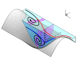
The present study simplified the dunes as three-dimensional staggered wavy walls, as shown in figure 1. The wall is characterized by an additional wave superimposed on the two-dimensional wavy wall in the spanwise direction. The geometric expression of the wall boundary is
 \begin{equation} \eta = a\sin ({2{\rm \pi} x}/{{{\lambda }_{x}}})\cos ({2{\rm \pi} y}/{{{\lambda }_{y}}}), \end{equation}
where  $a$ is the amplitude of the wavy wall and ${{\lambda }_{x}},{{\lambda }_{y}}$ are the wavelengths in the streamwise and spanwise directions.

Figure 1. Three-dimensional staggered wavy wall.
2.2 The LES model
The present paper uses LES to simulate the three-dimensional staggered wavy-wall turbulence. The filtered three-dimensional incompressible Navier–Stokes equations in Cartesian coordinates are
 \begin{gather} \frac{\partial {{u}_{i}}}{\partial {{x}_{i}}} = 0, \end{gather}
 \begin{gather}\frac{\partial {{u}_{i}}}{\partial t} + {{u}_{j}}\frac{\partial {{u}_{i}}}{\partial {{x}_{j}}} = {-}\frac{1}{\rho }\frac{\partial p}{\partial {{x}_{i}}} + \nu \frac{{{\partial }^{2}}{{u}_{i}}}{\partial {{x}_{j}}\partial {{x}_{j}}}-\frac{\partial {{\tau }_{ij}}}{\partial {{x}_{j}}} + f{{\delta }_{1i}}, \end{gather}
where  ${{x}_{i}}(i=1,2,3)=(x,y,z)$, respectively, denote the streamwise, spanwise and vertical coordinates, ${{u}_{i}}(i=1,2,3)=(u,v,w)$ denotes the filtered velocity components, $p$ is the filtered pressure, $f$ is the external force driving the flow, ${{\delta }_{ij}}$ is the Kronecker delta, $\nu$ is the kinematic viscosity, $\rho$ is the density and ${{\tau }_{ij}}$ is the subgrid-scale stress tensor. In the present study, the dynamic one-equation model is used as a subgrid-scale model (Reference Kim and MenonKim & Menon, 1995). Our previous work (Reference Zhang, Wang and LiuZhang et al., 2021; Reference Zhang, Wu, Liu and WangZhang, Wu, Liu, & Wang, 2022) has verified the numerical model according to the experimental results by Reference Hamed, Kamdar, Castillo and ChamorroHamed et al. (2015), suggesting the current LES is reliable.
2.3 Simulation configuration
Two groups, including 11 cases, are simulated to study the shape effect on the three-dimensional staggered wavy-wall turbulence. Group 1, which fixes the ratio of streamwise to spanwise wavelength, varies the ratio of the amplitude to the streamwise wavelength, while group 2 varies the ratio of streamwise to spanwise wavelength and fixes the amplitude. The shape parameters are presented in table 1. For group 1, the computational domain is  $({x}/{{{\lambda }_{x}}},{y}/{{{\lambda }_{y}}},{z}/{H})=( 2,2,1)$, where $H$ is the channel height. For group 2, due to the spanwise-wavelength variation, the domain length is $8{\lambda }_{y}$, $4{\lambda }_{y}$ and $2{\lambda }_{y}$ along the spanwise direction for cases G2-1 to G2-3. Whereas the length for cases G2-4 to G2-6 is ${\lambda }_{y}$. Based on our previous work (Reference Zhang, Wang and LiuZhang et al., 2021), the domain is sufficiently large to capture turbulent structures. The Reynolds number based on the bulk velocity and half-height of the channel is $Re={{{U}_{0}}h}/{\nu =4000}$, which provides fully developed turbulence. The flow is driven by the external force, which is transformed into a time-varying pressure gradient to fix the bulk velocity. To avoid the different measurements of velocity, most experiments in wind tunnels considered the blockage ratio to ensure accurate results. In the present paper, to avoid the sidewall effect on the flow, we applied periodic conditions along the streamwise and spanwise directions, and no-slip boundary conditions are applied to the upper and bottom walls. The grid points are evenly spaced in both the streamwise and spanwise directions. In the vertical direction, grid points are clustered at the boundary through an exponential transformation to enhance the accuracy of the boundary layer. The present study solved the flow on a body-fitted grid. The total number of the grid points for group 1 is ${{N}_{x}}\times {{N}_{y}}\times {{N}_{z}}=101\times 101\times 181$; in group 2 for G2-4 and G2-6, the grid point number is ${{N}_{x}}\times {{N}_{y}}\times {{N}_{z}}=101\times 76\times 181$ and ${{N}_{x}}\times {{N}_{y}}\times {{N}_{z}}=101\times 126\times 181$. The dimensionless grid scales are shown in table 1. Table 1 also gives resolved quantities, such as the momentum thickness of the boundary layer ${{\delta }_{m}}$, which refers to the thickness in which momentum is lost compared with that of a flat-wall boundary layer flow. To distinguish where the centrifugal-induced flow instability is, we here use the momentum thickness to visualize the region for generating the Görtler vortices (see details in § 4.2). The current grid scales meet the need for quasi-direct numerical simulation. We also evaluate the sub-grid-scale quantity and find that it is two orders of magnitude less than the resolved quantity, and we thus ignore its effect. The flow was simulated through 80 flow periods, with the initial 15 periods for turbulence development and the last 65 periods for statistical analysis. The time step was set as 30 viscous times ( ${30\nu }/{U_{0}^{2}}$), with approximately 16 000 instantaneous snapshots for the statistical analysis.
Table 1. The parameter settings for different cases.

3. Features of the secondary flows
3.1 Time-averaged velocity and swirling strength at cross-sections
Figure 2 shows the time-averaged streamwise velocity  ${{\bar {u}}}/{{{U}_{0}}}$ at the trough cross-sections with ${x}/{{{\lambda }_{x}}=0.75}$, with the vectors of time-averaged spanwise and vertical velocities also depicted. The flow separates in the streamwise direction, low-momentum fluids thus occupy the trough and form a convex feature at cross-sections. According to the vectors, the secondary flows possess similar directionality in transferring the flow from the crest into the trough. This results in the upwash (downwash) motion appearing at the crest (trough), which corresponds to the LMPs (HMPs). Several studies revealed that the low-momentum fluids are ejected into the upper averaged flow at the elevated region, while the downwash motion occurs in the recessed region (Reference Barros and ChristensenBarros & Christensen, 2014; Reference Chan, MacDonald, Chung, Hutchins and OoiChan, MacDonald, Chung, Hutchins, & Ooi, 2018; Reference HinzeHinze, 1967; Reference Mejia-Alvarez and ChristensenMejia-Alvarez & Christensen, 2013). However, for staggered wavy walls, transverse flow along the topography contributes to the unique upwash or downwash motion-induced momentum variation. The near crest's low-momentum fluids were lifted away from the wall, driven by the secondary flows and diving into the trough. As shown in figure 2, this leads to the convex momentum deficit pattern.

Figure 2. The contours of time-averaged streamwise velocity  ${{\bar {u}}}/{{{U}_{0}}}$, the vector of $({{\bar {v}}}/{{{U}_{0}}},{{\bar {w}}}/{{{U}_{0}}})$ shows the secondary flows; (a–f) for group 1 and (g–l) for group 2.
The amplitude effect is reflected in changing the low-velocity region, as shown in figure 2(a–f), with an enlarged momentum deficit region as the amplitude increases. This arises because of the enhancement of streamwise flow separation and transverse flow. Moreover, the scales of secondary flows are larger with the increase of wave amplitude, leading to clearer HMPs. Figure 2(g–l) shows how the spanwise wavelength affects the momentum transfer. The momentum deficit region enlarges vertically for a high spanwise-wavelength case with a wavy spatial pattern. This is related to the reduction of secondary flows in magnitude and scale. Moreover, the obscure momentum pathways can be seen as the increases in spanwise wavelength, as shown in figure 2(g) for case G2-1, at the position of  ${y}/{{{\lambda }_{y}}}=0$, the momentum pathways near the trough show a reversed direction compared with that far away from the trough vertically. However, for case G2-6, the upwash or downwash motion is dispersed along the spanwise direction.
The time-averaged velocity vectors show the macro-features of the large-scale secondary flows but cannot describe the vortex motions. To accurately visualize the strength of vortices at the cross-sections, figure 3 shows the time-averaged swirling strength  ${{\bar {\lambda }}_{ci}}$ (that in group 1 is made dimensionless by ${{{U}_{0}}}/{{{\lambda }_{x}}}$, while that in group 2 is made dimensionless by ${{{U}_{0}}}/{a}$) at the cross-section ${x}/{{{\lambda }_{x}}=0.75}$. Here, the swirling strength is defined as the imaginary part of the complex eigenvalue of the time-averaged velocity gradient tensor (Reference Zhou, Adrain, Balachandar and KendallZhou, Adrain, Balachandar, & Kendall, 1999). The present paper uses a two-dimensional velocity gradient tensor ( $\left [\begin {smallmatrix} {\partial \bar {v}}/{\partial y} & {\partial \bar {v}}/{\partial z} \\ {\partial \bar {w}}/{\partial y} & {\partial \bar {w}}/{\partial z} \end {smallmatrix}\right ]$) to capture the streamwise component of the swirling strength. We take an approach similar to that adopted by Reference Wu and ChristensenWu and Christensen (2006) and Reference Anderson, Barros, Christensen and AwasthiAnderson et al. (2015) in that the direction of the swirl, either clockwise ( ${{\bar {\lambda }}_{ci}}>0$) or anticlockwise ( ${{\bar {\lambda }}_{ci}}<0$), is obtained by multiplying the swirling strength by the sign of the time-averaged streamwise vorticity ( ${{\bar {\omega }}_{x}}={\partial \bar {w}}/{\partial y}-{\partial \bar {v}}/{\partial z}$). As can be seen, the swirling strength (primary counter-rotating vortex pair, denoted by primary CVP in the figure) above the trough is reversed compared with the small-scale vortex structure (secondary counter-rotating vortex pair, denoted secondary CVP in the figure) in the near trough region. In other words, the primary CVP induces upwash motion, while the secondary CVP induces downwash motion. It is noted that the near-wall small-scale vortex structure is unfavourable to the momentum transfer due to the enhanced shear effect on the wall boundary via downwash motion (Reference Dong and MengDong & Meng, 2004; Reference Hamed, Pagan-Vazquez, Khovalyg, Zhang and ChamorroHamed, Pagan-Vazquez, Khovalyg, Zhang, & Chamorro, 2017; Reference Lögdberg, Fransson and AlfredssonLögdberg, Fransson, & Alfredsson, 2009; Reference Medjoun, Vanderwel and GanapathisubramaniMedjoun et al., 2020).

Figure 3. The contours of mean swirling strength multiplied by the sign of mean streamwise vorticity; (a–f)  ${{{{\bar {\lambda }}}_{ci}}{{\lambda }_{x}}}/{{{U}_{0}}}$ for group 1; (g–l) ${{{{\bar {\lambda }}}_{ci}}a}/{{{U}_{0}}}$ for group 2. The solid box represents the integration region for small-scale swirling strength (secondary CVP) and the dashed box denotes the integration region for large-scale swirling strength (primary CVP).
With the increases in wave amplitude, as shown in figure 3(a–f), the swirling strength in the trough region enhances both the magnitude and scale. Whereas, as the spanwise wavelength increases, the swirling strength weakens, as shown in figure 3(g–l). Moreover, it is seen that the low level of swirling strength is dispersed at cross-sections.
It is noted that the results in figures 2 and 3 are not entirely symmetric. We here believe that the computational time and samples are adequate according to our simulation configuration. In the present paper, the secondary flow was captured based on the time-averaged field, which was regarded as an artefact. We checked the instantaneous field and found that the secondary flow structures are relatively regular at the initial stage. However, a periodic condition develops turbulence, which means that the secondary flow is generated through inflow with turbulence after the turbulence is fully developed. Inspired by the instantaneous field, we suggested that the instantaneous vorticity under the strain effect results in its stretch or rotation. Therefore, the initial streamwise vortices are likely to rotate into spanwise or vertical vorticity through the strain rate tensor. Similarly, the spanwise vorticity may be transformed into streamwise vorticity via the strain effect. This leads to the inclusion of the spanwise vorticity-induced streamwise vorticity in the total streamwise vorticity after time averaging. We also considered the following reason: the flow is strongly three-dimensional, and enough spatial averaging of the mean field at different cross-sections would lead to a more symmetric feature of the velocities.
From figure 3, there is a certain qualitative relation between the swirling strength and shape parameters. To further construct this relation, we integrate the swirling strength in designated regions at cross-sections to obtain the local mean swirling strength. As shown in figure 3(a), the integration region in the trough stretches across approximately  $\frac {3}{8}{{\lambda }_{y}}$, with the vertical boundary expanding into $z\approx a$. The integral region above the crest stretches across $\frac {5}{8}{{\lambda }_{y}}$, with the vertical boundary at $z\approx 0.4H$. Here, the upper limit of integration is determined based on the region with the wall effect. The mean swirling strength is expressed as
 \begin{equation} \left\{\begin{gathered} I_{{{{\bar{\lambda}}}_{ci}}}^{1,t} = \frac{1}{{{R}_{t}}} \int_{\eta }^{a}{\int_{-({3}/{16}){{\lambda }_{y}}}^{({3}/{16}){{\lambda }_{y}}}{ \left| {{{{\bar{\lambda}}}_{ci}}{{\lambda }_{x}}}/{{{U}_{0}}}\right|}}{\rm d} y\,{\rm d} z,\quad {x}/{{{\lambda }_{x}} = 0.75}\\ I_{{{{\bar{\lambda}}}_{ci}}}^{2,t} = \frac{1}{{{R}_{t}}}\int_{\eta }^{a} {\int_{-({3}/{16}){{\lambda }_{y}}}^{({3}/{16}){{\lambda }_{y}}}{ \left| {{{{\bar{\lambda}}}_{ci}}a}/{{{U}_{0}}}\right|}}{\rm d} y\,{\rm d} z,\quad {x}/{{{\lambda }_{x}} = 0.75} \\ I_{{{{\bar{\lambda}}}_{ci}}}^{1,c} = \frac{1}{{{R}_{c}}}\int_{\eta }^{0.4H} {\int_{-({5}/{16}){{\lambda }_{y}}}^{({5}/{16}){{\lambda }_{y}}}{\left| {{{{\bar{\lambda}}}_{ci}} {{\lambda }_{x}}}/{{{U}_{0}}}\right|}}{\rm d} y\,{\rm d} z,\quad {x}/{{{\lambda }_{x}} = 0.25} \\ I_{{{{\bar{\lambda}}}_{ci}}}^{2,c} = \frac{1}{{{R}_{c}}}\int_{\eta }^{0.4H}{\int_{-({5}/{16}) {{\lambda }_{y}}}^{({5}/{16}){{\lambda }_{y}}}{\left| {{{{\bar{\lambda}}}_{ci}}a}/{{{U}_{0}}}\right|}}{\rm d} y\,{\rm d} z,\quad {x}/{{{\lambda }_{x}} = 0.25} \end{gathered}\right., \end{equation}
where the superscript 1 or 2 represents group 1 or 2. Here,  $t$ and $c$ denote the region in the trough or crest, and ${{R}_{t}}$ ( ${{R}_{c}}$) is the area of the integral region in the trough (crest).
Figure 4 shows the mean swirling strength curves varying with the amplitude or spanwise wavelength. The dashed line in the figure represents the flat-wall boundary layer flow under idealized conditions (the streamwise swirling strength is zero). As shown in figure 4(a,c), the mean swirling strength is enhanced as the amplitude increases in both the trough and crest regions. For group 2 shown in figure 4(b,d), the mean swirling strength decreases with the rise of the spanwise wavelength. Figure 4 also suggests that the mean swirling strength varies more strongly with the amplitude than the spanwise wavelength, which indicates the domination of the amplitude effect.

Figure 4. The mean swirling strength at the region of trough or crest for two groups.
The integration mentioned above contains large-scale vortices (primary CVP) and small-scale vortices (secondary CVP). To separately discuss their dependence on the wall characteristic parameters, we further integrate the swirling strength in a different designated region, as shown in figure 3 by the solid or dashed boxes. Figure 5 shows the mean swirling strength  $[\bar {\lambda }_{ci}^{+}]$ for large-scale and small-scale vortices. Generally, increased $[\bar {\lambda }_{ci}^{+}]$ with rising amplitude can be found for both large-scale and small-scale vortices. Whereas, for group 2, $[\bar {\lambda }_{ci}^{+}]$ is enhanced and then decreases with the spanwise wavelength, indicating a swirling strength peak for the case with ${{{\lambda }_{y}}}/{{{\lambda }_{x}}}=1$ (noting that, for case G2-1, due to the limitation of the spanwise wavelength, we cannot capture the small-scale vortices).

Figure 5. Mean swirling strength for large-scale ( $M_l$) and small-scale ( $M_s$) vortices varying with the wall parameters.
According to the time-averaged velocity and swirling strength, the mechanism of secondary flows can be further revealed. When flowing through a three-dimensional staggered wavy wall, the concave trough is filled with low-velocity fluids, thus forming the convex low-momentum region. As shown in figure 6, the isoline of zero streamwise velocity possesses a similar feature to a real convex wall, consequently leading to secondary flow with upwash motion. The reversed flow in this momentum deficit region could induce secondary flow with a downwash motion. Therefore, two different momentum pathways can be found in the trough region, which reveals that both LMPs and HMPs are in the recessed region.

Figure 6. Sketch of the secondary flows at the trough.
3.2 Streamwise variation of the time-averaged streamwise vorticity
This section emphasizes the streamwise variation of the time-averaged streamwise vorticity. To clarify the macro-swirling strength at cross-sections, we calculate the mean streamwise vorticity  ${{\varGamma }^{+}}$ to characterize the strength of the streamwise vortices. The dimensionless mean streamwise vorticity is determined in a way similar to that of Reference Medjoun, Vanderwel and GanapathisubramaniMedjoun et al. (2020)
 \begin{equation} {{\varGamma }^{ + }} = \frac{1}{I_A}\int_{\eta }^{0.3H} {\int_{{-}0.5{{\lambda }_{y}}}^{0.5{{\lambda }_{y}}}{|{{{\bar{\omega}}}_{x}}}}{{|}^{ + }}\,{\rm d} y\,{\rm d} z, \end{equation}
where  $I_A$ denotes the integral region at cross-sections. The + means that the vorticity is dimensionless by ${{{\lambda }_{x}}}/{{{U}_{0}}}$ or ${a}/{{{U}_{0}}}$ for group 1 or 2. We set the upper limit as $0.3H$, owing to the large-scale secondary flows concentrated within this region. Moreover, the three-dimensional staggered wavy wall is of zero average wall elevation at any cross-section. Therefore, the area of the integration region at different cross-sections remains the same.
Figure 7 shows the variation curves of mean streamwise vorticity along the streamwise direction. As shown in figure 7(a,b), the mean streamwise vorticity shows periodic variation, with two peaks appearing near  ${x}/{{{\lambda }_{x}}\approx 0.5,1}$, corresponding to where the bottom boundary possesses zero spanwise curvature. Moreover, as demonstrated by the vorticity contour on these cross-sections, there is symmetrical high-level vorticity near the wall boundary. These enhanced vorticities suggest that these regions might be the origin of formation of the streamwise vortices.

Figure 7. Streamwise variation curves of the vorticity for the two groups.
4. Formation of the streamwise vortices
4.1 Instantaneous streamwise vortices
The streamwise vortices are accompanied by secondary flows. This section emphasizes the morphological features of the streamwise vortices. Figure 8 visualizes the instantaneous vortex structures via the  ${{\lambda }_{2}}$ method (Reference Jeong and HussainJeong & Hussain, 1995), where (a) shows the case G1-4 and (b) shows the case G1-6. There are typical horseshoe vortex structures near the crest, as shown by A in the figure. The disruption of coherent structures is stronger when the amplitude increases and the vortices in the near-wall region are more concentrated in case G1-6 than in case G1-4. Additionally, the vortices highly meander vertically with the increases of amplitude. Hence, the amplitude modulates the vertical momentum transfer by adjusting the meandering of the vortices.

Figure 8. Instantaneous vortex structures of  ${{\lambda }_{2}}=-10$ for (a) G1-4 and (b) G1-6.
The effect of spanwise wavelength on instantaneous vortices is shown in figure 9, where (a) shows the case G2-3 and (b) the case G2-6. The vortices are visualized by  ${{\lambda }_{2}}=-5$ due to the magnitude and scale of streamwise vortices being weaker compared with the cases in group 1; the lower value of ${{\lambda }_{2}}$ can depict the macro-feature of the vortex structures. At the position shown by the red dashed line in figure 9, there are rare vortices due to the zero streamwise curvature of the wall boundary (Reference Zedler and StreetZedler & Street, 2001). The vortices mainly appear near the crest and expand downstream, with spanwise meandering behaviour. As shown in case G2-3, the streamwise vortices are generated ahead of the crest and are gradually spanwise bent to flow around the crest. The spanwise wavelength could adjust the spanwise-bent extent of the streamwise vortices, as shown in figure 9(b), where the streamwise vortices are less spanwise bending for large spanwise-wavelength cases, and the scale of these vortices enlarges along the streamwise direction. Therefore, the spanwise wavelength controls the spanwise bending of the streamwise vortices, consequently modulating the spanwise component of momentum transport.

Figure 9. Instantaneous vortex structures of  ${{\lambda }_{2}}=-5$ for (a) G2-3 and (b) G2-6. The red dashed lines denote the positions crossinglines of zero streamwise curvature.
4.2 Potential centrifugal instability and Görtler number
Figures 8 and 9 show that the morphological features of streamwise vortices depend on the shape parameter of the wall. For two-dimensional concave wall turbulence, the streamlines are curved and thus generate streamwise vortices via the centrifugal instability. Nevertheless, the curvature of streamlines for the present three-dimensional staggered wavy wall turbulence shows three-dimensionality, which might lead to a complex centrifugal instability. In a two-dimensional turbulent flow, the potentially unstable regions can be distinguished by the Rayleigh criterion (Reference Beaudoin, Cadot, Aider and WesfreidBeaudoin, Cadot, Aider, & Wesfreid, 2004; Reference SaricSaric, 1994). Here, we consider the three-dimensional Rayleigh criterion
 \begin{equation} \left\{\begin{gathered} {{\phi }_{xy}} = \frac{2|\boldsymbol{\bar{u}}|{{{\bar{\omega}}}_{z}}}{{{R}_{xy}}} \\ {{\phi }_{xz}} = \frac{2|\boldsymbol{\bar{u}}|{{{\bar{\omega}}}_{y}}}{{{R}_{xz}}} \end{gathered}\right., \end{equation}
where  $| {\boldsymbol {\bar {u}}} |$ is the modulus of the time-averaged velocity, and ${{\bar {\omega }}_{y}}$ and ${{\bar {\omega }}_{z}}$ denote the time-averaged spanwise and vertical vorticity, respectively; ${{R}_{xy}}$ ( ${{R}_{xz}}$) represents the algebraic radius of curvature based on the time-averaged velocity vector $( \bar {u},\bar {v} )$ ( $(\bar {u},\bar {w} )$), which can be calculated by
 \begin{equation} \left\{\begin{gathered} {{R}_{xy}} = \frac{|\boldsymbol{\bar{u}}{{|}^{3}}}{\bar{u}{{a}_{y}}-\bar{v}{{a}_{x}}} \\ {{R}_{xz}} = \frac{|\boldsymbol{\bar{u}}{{|}^{3}}}{\bar{u}{{a}_{z}}-\bar{w}{{a}_{x}}} \end{gathered}\right., \end{equation}
where  ${{a}_{x}},{{a}_{y}}, {{a}_{z}}$ are the components of the convective acceleration calculated from $( \boldsymbol {\bar {u}}\boldsymbol {\cdot }\boldsymbol {\nabla })\boldsymbol {\bar {u}}$. According to the Rayleigh criterion, the flow could be potentially unstable if the local radius of curvature is reversed in sign compared with the vorticity.
Figure 10 shows the potentially unstable regions for case G1-2, where the regions A–D in figure 10(a) denote the unstable region on the  $x$–
$x$– $z$ plane, while regions E–H in figure 10(b) are the unstable regions on the characteristic $x$–
$x$– $y$ plane. The streamlines visualize the flow separation on both longitudinal–vertical and horizontal cross-sections. The flow on the former plane separates behind the crest and then reattaches on the windward side. However, there are two separations behind the crest and reattachments ahead of the downstream crest on the latter plane. It is noted that, under idealized conditions, the flow separation and reattachment on the horizontal cross-section are symmetrical. However, due to the strong three-dimensional flow, the results cannot be entirely symmetrical. We here also believe that enough spatial averaging for different cross-sections may result in a more symmetrical result. Reference Marxen, Lang, Rist, Levin and HenningsonMarxen, Lang, Rist, Levin, and Henningson (2009) suggested that the curved streamline effect above the separation bubble is similar to that of a concave wall boundary in the generation of Görtler vortices (streamwise vortices). For the current cases, the streamlines near the separation and reattachment points on both longitudinal–vertical and horizontal cross-sections might induce streamwise vortices due to the curvature effect.

Figure 10. The contour of the Rayleigh criterion for case G1-2; (a) A, B, C and D are potentially unstable regions and (b) E, F, G and H are potentially unstable regions.
However, the Rayleigh criterion gives the necessary condition for centrifugal instability while ignoring the stability condition by the viscous effect. Therefore, there is a requirement for evaluating the Görtler number characterized by the ratio of the centrifugal effect to the viscous effect to distinguish the region where the flow could induce streamwise vortices. The Görtler number for current three-dimensional cases is expressed as
 \begin{equation} \left\{\begin{gathered} {{G}_{xz}} = \frac{|\boldsymbol{\bar{u}}|\delta _{m}^{{3}/{2}}}{\nu R_{xz}^{{1}/{2}}} \\ {{G}_{xy}} = \frac{|\boldsymbol{\bar{u}}|\delta _{m}^{{3}/{2}}}{\nu R_{xy}^{{1}/{2}}} \end{gathered}\right., \end{equation}
where  ${{\delta }_{m}}$ is the momentum thickness of the boundary layer shown in table 1.
Figure 11 shows the Görtler number on longitudinal–vertical and horizontal cross-sections for cases G1-2, G1-6 and G2-6, located at  ${y}/{{{\lambda }_{y}}}=0$ and ${z}/{a}=0.5$ (in the following discussions, YS0 denotes the former's longitudinal–vertical section while ZS1 represents the latter's horizontal section.). The results suggest that high ${{G}_{xz}}$ appears at the separation and reattachment points and exceeds the threshold value for generating streamwise vortices (according to Reference TobakTobak (1971) and Reference IngerInger (1987), the criteria for centrifugal-induced Görtler vortices is ${{G}_{xz}}\ge 0.25$). A larger amplitude enhances the value of ${{G}_{xz}}$, as shown in figure 11(b). This is due to the higher curvature of the streamlines. It is also found that the Görtler number in region A is much smaller than that in region B, indicating reattachment-dominated centrifugal instability, as verified for the two-dimensional wavy-wall case in our previous work (Reference Zhang, Wu, Liu and WangZhang et al., 2022). The Görtler number on ZS1 ( ${z}/{a}=0.5$) could represent a region that can easily generate streamwise vortices because ZS1 possesses the largest potentially unstable regions, as shown in figure 10. In figure 11(d,e), ${{G}_{xy}}$ is less in regions E and F than in regions G and H. However, ${{G}_{xy}}$ reaches the threshold value for generating streamwise vortices, which suggests the origins of the streamwise vortices. It is noted that, although there is a high ${{G}_{xy}}$ around the crest extending downstream, these regions cannot entirely represent the origins of the streamwise vortices. In other words, the transverse flow around the near-hill region can be equivalent to the flow over a convex wall, which is stable. However, modulated by the topography, this flow not only passes across the back of the hill but also into the oblique rear's hill. This results in the unstable region appearing near the oblique rear's hill, corresponding to the regions G and H in figure 10. Moreover, the higher amplitude would not change the fundamental feature of ${{G}_{xy}}$ while increasing its magnitude.

Figure 11. The distribution of Görtler number at YS0 section ( ${y}/{{{\lambda }_{y}}}=0$) for (a) G1-2, (b) G1-6 and (c) G2-6. The distribution of Görtler number at ZS1 section ( ${z}/{a}=0.5$) for (d) G1-2, (e) G1-6 and (f) G2-6.
The centrifugal effect for inducing streamwise vortices is also influenced by the variation of spanwise wavelength. The higher spanwise wavelength mainly affects the Görtler number at the separation point, and the range of relatively high  ${{G}_{xz}}$ is narrowed, as shown in figure 11(a,c). This reveals that the strength of streamwise vortices is weaker for two-dimensional wavy-wall cases than that for three-dimensional staggered wavy wall cases (Reference Zhang, Wang and LiuZhang et al., 2021). On the ZS1 section, as shown in figure 11(d,f), increasing the spanwise wavelength weakens ${{G}_{xy}}$, related to decreased streamline curvature.
Furthermore, we correlate the Görtler number with the shape parameters. Figure 12 shows the local-averaged Görtler number as a function of two shape parameters. The local-averaged Görtler number is determined by the integration in a specific region, expressed as
 \begin{equation} \left\{\begin{gathered} G_{xz-A}^{la} = \int_{A}{{{G}_{xz}}\,{\rm d} A} \\ G_{xy-E}^{la} = \int_{E}{{{G}_{xy}}\,{\rm d} E} \\ G_{xz-B}^{la} = \int_{B}{{{G}_{xz}}\,{\rm d} B} \\ G_{xy-G}^{la} = \int_{G}{{{G}_{xy}}\,{\rm d} G} \\ G_{xz}^{la} = \int_{{{\varOmega }_{xz}}}{{{G}_{xz}}\,{\rm d} {{\varOmega }_{xz}}} \\ G_{xy}^{la} = \int_{{{\varOmega }_{xy}}}{{{G}_{xy}}\,{\rm d} {{\varOmega }_{xy}}} \end{gathered}\right., \end{equation}
where  $A$ is enclosed by ${{\phi }_{xz}}=-0.5$, $E$ is enclosed by ${{\phi }_{xy}}=-0.5$, $B$ is enclosed by ${{\phi }_{xz}}=-0.2$ and $G$ is enclosed by ${{\phi }_{xy}}=-0.2$. It is noted that the potentially unstable region at the ZS1 section features a lower $| {{\phi }_{xy}} |$, we thus integrated the Görtler number in the designated region enclosed by ${{\phi }_{xy}}=-0.5$ and ${{\phi }_{xy}}=-0.2$. Therefore, we can strictly compare the local-averaged Görtler number in regions A and E and regions B and G. Further, ${{\varOmega }_{xz}}$ indicates the region in the YS0 section enclosed by ${{\phi }_{xz}}<0$, and ${{\varOmega }_{xy}}$ denotes the region in ZS1 section enclosed by ${{\phi }_{xy}}<0$. It is noted that the centrifugal instability at the ZS1 section is symmetrical with the wavy topography, while the centrifugal instability induces vortices mainly located within the near-wall region at the YS0 section, therefore, we here use the region with ${z}/{H}< a/\lambda _x$ at the YS0 section for integration, which is located approximately at the core region of the enhanced Görtler number. It is shown in figure 10 that the isoline of ${{\phi }_{xy}}=0$ appears near ${y}/{{{\lambda }_{y}}}=\pm 0.25$, dividing the high Görtler number region into two parts across the enhancement core. Therefore, a comparison of the Görtler number between the YS0 and ZS1 sections can be established.

Figure 12. Local-averaged Görtler number at the YS0 and ZS1 sections and regions A, E, B and G for different cases. (a) Group 1, (b) group 2.
Figure 12(a) shows the local-averaged Görtler number varying as a function of wave slope. As can be seen, a higher amplitude increases the Görtler number. Moreover, it is found that lower (higher) amplitude leads to the domination of the centrifugal instability on the horizontal (longitudinal–vertical) cross-sections. Near the separation point,  $G_{xz-A}^{la}$ in region A is less than $G_{xy-E}^{la}$ in region E, indicating that the streamwise vortices behind the crest are readily generated through the centrifugal instability on the horizontal cross-section. In regions B and G, it is found that $G_{xy-G}^{la}$ is higher than $G_{xz-B}^{la}$, which means the flow reattachment-induced centrifugal instability is stronger on the horizontal cross-section. It can also be demonstrated in figure 11 that the Görtler number at the ZS1 section is higher than that at the YS0 section. Figure 12(b) illustrates the local-averaged Görtler number varying as a function of the spanwise- to streamwise-wavelength ratio. Generally, the effect of spanwise wavelength is not as significant as the amplitude. It is seen that the centrifugal instability on the longitudinal–vertical cross-section dominates with the increase in the spanwise wavelength. Furthermore, the centrifugal instability appears more readily near the separation through the transverse flow. However, the relative strength of the Görtler number at different sections relies on the present spanwise wavelength. It is shown in figure 12(b) that $G_{xy-G}^{la}$ first increases and then decreases with the rising spanwise wavelength while $G_{xz-B}^{la}$ shows a rising trend, resulting in a centrifugal instability dominated by flow reattachment on the longitudinal–vertical cross-section. It is worth noting that, when ${{{\lambda }_{y}}}/{{{\lambda }_{x}}}=1$, there is a peak of the local-averaged Görtler number, which means the streamwise vortices can be generated most easily on the horizontal cross-section.
5. Concluding remarks
In the present paper, a large-eddy simulation has been conducted to investigate the secondary flows and streamwise vortices in three-dimensional staggered wavy-wall turbulence with different shape parameters. Based on the ratio of spanwise heterogeneity to the boundary layer thickness, most cases in the present paper can be characterized as topography regimes. The large-scale secondary flows were captured by calculating the swirling strength through the complex eigenvalue of the time-averaged velocity gradient tensor. After comparing time-averaged velocities and swirling strength, the formation of LMPs (HMPs) caused by the secondary flow-induced upwash (downwash) motion is discussed. Then, the centrifugal instability criterion revealed the generation mechanism of the streamwise vortices.
The present shape parameters of a three-dimensional staggered wavy wall determine the strength of the secondary flows. Higher amplitude (spanwise wavelength) enhances (weakens) the secondary flows. The position for generating secondary flows is related to the momentum variation induced by flow separation. Generally, the momentum deficit by flow separation occupies the trough region, with convex curvature of the zero isolines of the streamwise velocity as a pseudo-wall in inducing the secondary flow with upwash motion (LMPs); however, affected by the concave trough and the turbulent shear layer with concave curvature, the reversed flow generates secondary flows with downwash motion (HMPs). This reveals there are both LMPs and HMPs in the recessed region.
The streamwise vortices cater to the wall boundary by adjusting their bending degree. Higher amplitude (spanwise wavelength) enhances (weakens) the vertical (transverse) bending feature of the vortices. The streamwise vortices are generated via centrifugal instability on longitudinal–vertical and horizontal cross-sections, with that on the former section triggered by the curved separated shear layer, whereas that on the latter section is induced by the curved shear layer when flowing around the crest. The separation and reattachment points in both sections are confirmed as the origins of the streamwise vortices. By evaluating the maximum ratio of the centrifugal effect to the viscous effect, when fixing the ratio of spanwise to streamwise wavelength, the instability on the longitudinal–vertical cross-section gradually dominates with the increase in amplitude. This can also be found for the cases with spanwise-wavelength variation. It is found that the streamwise vortices are generated more readily through transverse flow around the crest near the separation and reattachment points whereas for the large spanwise-wavelength cases, the centrifugal instability by flow reattachment on the longitudinal–vertical cross-section dominates. It is worth noting that, for transverse flow-induced instability on the horizontal cross-section, the streamwise vortices are generated most easily when the ratio of spanwise to streamwise wavelength equals 1.
The present paper reveals the mechanism of secondary flow-induced momentum pathways and how centrifugal instability generates streamwise vortices in turbulent flow over large-scale three-dimensional staggered wavy walls. However, the present investigations raise some unresolved problems. In the natural sand terrain, the dunes feature a variety of shapes due to the different flow regimes, such as dunes resulting from unidirectional flow and ripples by oscillatory flow. The present simplification is reasonable to some extent, but cannot entirely reflect real naturally developed dunes. A systematic comparison of flow over the different kinds of dunes should be investigated. Moreover, there are turbulent flows and sediment transport. These multi-physical processes dominate the geomorphology dynamics. How these processes affect the evolution of the dunes should be investigated to figure out the internal mechanism of turbulent sediment transfer.
Supplementary material
Raw data are available from the corresponding author (L.Q.Q.).
Acknowledgements
The research meets all ethical guidelines, including adherence to the legal requirements of the study country.
Funding statement
This work was supported by the National Natural Science Foundation of China (nos 12032005, 12172057, 12002039) and the National Key R&D Program of China under grant number 2021YFA0719200.
Declaration of interests
The authors declare no conflict of interest.


 Open access