


Impact Statement
Large-amplitude internal waves are a primary conduit for transport across the boundary layer on continental shelves, and are contributors to horizontal transport. Being a non-hydrostatic phenomenon, such waves are beyond the reach of all global, and most regional, ocean models. This review contributes to our understanding of the gaps in existing models, and guides future work that can provide novel parametrizations for such models. It does so by surveying recent modelling, experimental and field work efforts. A number of different avenues for future work are identified, along with the reasons why these directions are scientifically profitable.
1. Introduction
Large-amplitude internal waves, often labelled as internal solitary waves (ISWs) or nonlinear internal waves, are a ubiquitous part of density stratified natural waters (e.g. Reference Preusse, Freistühler and PeetersPreusse, Freistühler & Peeters (2012) for lakes, Reference Pinkel, Merrifield, McPhaden, Picaut, Rutledge, Siegel and WashburnPinkel et al. (1997) for the deep ocean and Reference Quaresma, Vitorino, Oliveira and da SilvaQuaresma et al. (2007) and Reference Shroyer, Moum and NashShroyer, Moum & Nash (2009) for two examples for the coastal ocean). In the ocean, such waves are formed by a variety of mechanisms, the most common being the interaction of the barotropic tide with the topography. While ISW observations span the globe, studies are generally concentrated on a select number of regions of generation. Due to the generic nature of ISW generation, this suggests that the present documentation of ISW incidence under-reports their geographical distribution. Notably well-studied regions include the South China Sea (Reference Chang, Lien, Lamb and DiamessisChang et al. 2021), the Strait of Gibraltar (Reference Alpers, Brandt and RubinoAlpers, Brandt & Rubino 2008), the Portuguese Shelf (Reference Quaresma, Vitorino, Oliveira and da SilvaQuaresma et al. 2007), the California coast (Reference McSweeney, Lerczak, Barth, Becherer, Colosi, MacKinnon, MacMahan, Moum, Pierce and WaterhouseMcSweeney et al. 2020a,Reference McSweeneyb), the Australian Northwest Shelf (Reference Jones, Ivey, Rayson and KellyJones et al. 2020; Reference Zulberti, Jones and IveyZulberti, Jones & Ivey 2020) and the New Jersey Shelf (Reference Shroyer, Moum and NashShroyer et al. 2009). The geographic coverage of simulations is even more sparse as they are often idealized (i.e. not tied to a particular location).
In this review, the preferred acronym ISW will be used, however, we loosen the strict ‘solitariness’ to include what are often referred to as internal solitary-like waves. The need for this terminology will be discussed in what follows, but in essence the ocean is too dynamically active for a wave to meet the mathematical definition of the term ‘solitary’. Nevertheless, ISWs have been observed to propagate hundreds of kilometres without a profound change in shape. Their persistence of shape and finite amplitude imply that ISWs can be an efficient means to move material, including plankton, horizontally (Reference LambLamb 1997; Reference Scotti and PinedaScotti & Pineda 2007) and vertically (see Reference Bogucki, Dickey and RedekoppBogucki, Dickey & Redekopp (1997), Reference Quaresma, Vitorino, Oliveira and da SilvaQuaresma et al. (2007) as well as the review Reference Boegman and StastnaBoegman & Stastna (2019) for mechanisms and a broader literature review). Internal solitary waves are not the only type of finite-amplitude internal wave observed (e.g. solibores or dnoidal waves Reference ApelApel 2003), and indeed recent simulations of shoaling in a situation with very broad stratifications feature bores almost exclusively (Reference Dauhajre, Molemaker, McWilliams and HypoliteDauhajre et al. 2021).
A natural question to ask about ISWs is ‘where does the energy and momentum associated with such waves end up?’ Indeed for many ISWs, the final stage of their life cycle involves propagation into shallow water, a process referred to as shoaling. While superficially analogous to shoaling surface waves, internal wave shoaling occurs on much longer length scales, and in many situations is a gentle process. Shoaling is an example of how waves evolve as their environment (i.e. their waveguide) changes. Other examples involve the interaction of waves with currents and fronts (Reference Bogucki, Dickey and RedekoppBogucki et al. 1997; Reference Davies and XingDavies & Xing 2002), and interactions with eddies or long waves (Reference Dunphy and LambDunphy & Lamb 2014). During shoaling the waves change shape and begin to interact with the ocean bottom more strongly.
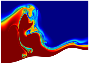
The features of the shoaling process are best explained with a visual example. The two-dimensional simulations of internal wave shoaling in the well-studied South China Sea shown in figure 1, reproduced with permission from Reference Lamb and Warn-VarnasLamb & Warn-Varnas (2015), will be used to illustrate some of these features. In these simulations, both a realistic stratification and a bathymetric transect are employed in a non-hydrostatic, second-order finite volume model (this model has been used for internal wave studies for several decades). The waves are followed from a region that is three kilometres deep to a shallow region that is of the order of one hundred metres deep. The waves undergo a complex, but mostly gentle, series of transformations. Several examples of phenomena generally accepted to be universal aspects of internal wave shoaling are evident. These include the evolution into multiple waves ( $t=42$ hours), the steepening of the rear face of the wave ( $t=50$ hours) and the formation of higher mode waves ( $t=58$ hours). More exotic phenomena such as the formation of flat-crested, or table-top, waves ( $t=58$, $66$ hours) are also evident.

Figure 1. The density field for simulations of shoaling internal waves in the South China Sea, reproduced from Reference Lamb and Warn-VarnasLamb & Warn-Varnas (2015) (their figure 4).
The complexity of the shoaling process, as shown in figure 1, has led to a pattern of simplification and idealization in simulations and laboratory work. Thus, in many studies the bathymetry, stratification and wave shape are as simple as possible. Figure 2, reproduced with permission from Reference Lamb and XiaoLamb & Xiao (2014), shows an example of internal wave shoaling for a model, quasi-two-layer stratification over a smooth hyperbolic tangent bathymetry. The case shown illustrates an incident wave of depression fissioning into a wave train of elevation waves. Like the process shown in figure 1, at no point does the process shown in figure 2 involve violent wave breaking or density overturns. It is important to note that the dynamics of the boundary layer is ignored in both the idealized (figure 2) and field-scale (figure 1) simulations.

Figure 2. Example of internal wave shoaling in the fissioning regime for a quasi-two-layer stratification. Reproduced from Reference Lamb and XiaoLamb & Xiao (2014) (their figure 8).
While the quasi-two-layer stratification brings simplicity, and has been utilized in some recent experimental work (Reference Ghassemi, Zahedi and BoegmanGhassemi, Zahedi & Boegman 2022), there has also been significant work that considers the effect of pycnocline location and thickness (Reference Allshouse and SwinneyAllshouse & Swinney 2020; Reference Hartharn-Evans, Carr, Stastna and DaviesHartharn-Evans et al. 2022; Reference Hartharn-Evans, Stastna and CarrHartharn-Evans, Stastna & Carr 2023). In particular, a thicker pycnocline has been found to significantly influence the properties of upstream propagating boluses (for example, figure 5 of Reference Hartharn-Evans, Stastna and CarrHartharn-Evans et al. (2023) contrasts the space–time behaviour for three stratifications). A different branch of the theoretical literature concerns explicitly layered stratifications (Reference Grue, Jensen, Rusås and SveenGrue et al. 1999, Reference Grue, Jensen, Rusaas and Sveen2000; Reference GrueGrue 2015) which yield some mathematical simplifications. The ocean can be expected to exhibit a complex, and possibly time-varying, stratification profile, and thus intuition developed based on quasi-two-layer stratifications should be used to interpret data carefully, and theories with a larger number of layers offer some hope for tying theory and observation together. Nevertheless, continuously stratified theories transfer more directly to the majority of ocean models since these are formulated from continuously stratified governing equations.
Regardless of the choice of stratification, the shoaling process itself is not always gentle. Reference LambLamb (2002) showed that, when large-amplitude waves shoal, wave breaking can be the dominant process, and that in the case of stratifications for which density monotonically decreases near the upper boundary, a recirculating core may form. Reference Grue, Jensen, Rusaas and SveenGrue et al. (2000) demonstrated experimentally that a recirculating region forms in waves developing from a lock release. In the case of large waves this region was quite active, and since physical experiments are limited by the tank length, it was not possible to determine if the core eventually settled to a quasi-steady form. The existence of a trapped core (assumed to not be circulating) was posited on theoretical grounds earlier (Reference Derzho and GrimshawDerzho & Grimshaw 1997), although Grue et al. were the first to demonstrate it experimentally, and Lamb was the first to outline an efficient process to determine when one might form naturally. Lamb was also able to classify stratifications which do or do not form cores. Since a mixed layer is commonly observed in the ocean, and precludes core formation, trapped cores were considered an interesting oddity for a number of years. This changed with the measurements of Reference Lien, D'Asaro, Henyey, Chang, Tang and YangLien et al. (2012), which demonstrated a clear subsurface core for an ISW propagating in the South China Sea. Simulations of the shoaling process that leads to the formation of such a core (Reference Rivera-Rosario, Diamessis, Lien, Lamb and ThomsenRivera-Rosario et al. 2020) are reproduced as figure 3. These clearly show that the core is long lived, efficiently traps fluid and exhibits an active circulation. Theoretical support for subsurface cores was provided in Reference He, Lamb and LienHe, Lamb & Lien (2019), and it was shown that the presence of a background shear current is essential. Indeed, the idea that a background shear current can change both the value of the limiting amplitude and the process that sets the limit (i.e. wave breaking versus wave broadening versus shear instability) dates back to work on exact ISWs over twenty years ago (Reference Stastna and LambStastna & Lamb 2002). It is interesting that experimental evidence (Reference Luzzatto-Fegiz and HelfrichLuzzatto-Fegiz & Helfrich 2014) suggests that, on laboratory scales, trapped cores have essentially zero velocities. We will return to this disparity in behaviour at laboratory and field scales at various points in the following. Nevertheless, it is important to note that cores, whether they are completely trapped or not, are likely the dominant ISW-related process as far as horizontal transport is concerned. It is for this reason that studying their spanwise structure, and the manner in which it may lead to fluid and transported material ‘leaking’ from the core, is a vital topic to address. To date the majority of modelling efforts have been two-dimensional.

Figure 3. Isopycnal contours at select locations during the ISW shoaling along a transect in the South China Sea. Four different snapshots correspond to different times after the start of the simulation at location I. (a) The wave prior to the wave-induced velocity surpassing the propagation speed, and the wave at the (b) subsurface and (c) surface mooring locations. (d) The ISW has reached the shallowest portion of the transect, i.e. location II. (e) The South China Sea transect, along with the placement of each snapshot. Reproduced from Reference Rivera-Rosario, Diamessis, Lien, Lamb and ThomsenRivera-Rosario et al. (2020) figure 7.
While trapped, or nearly trapped, cores could be quite energetic, with an active, three-dimensional structure, they have not been documented to lead to terminal ISW breakdown. Indeed, the breaking process associated with core formation should be contrasted with the breaking that occurs in the terminal phase of shoaling (upslope of where the main pycnocline intercepts the shelf). This region has been documented to lead to the generation of upslope propagating boluses (see for example Reference Richards, Bourgault, Galbraith, Hay and KelleyRichards et al. (2013) and Reference Lucas and PinkelLucas & Pinkel (2022) for field measurements, and Reference Wallace and WilkinsonWallace & Wilkinson (1988) and Reference Hartharn-Evans, Carr, Stastna and DaviesHartharn-Evans et al. (2022) for experiments).
The dynamics of internal waves in the ocean, including shoaling, has been the subject of several recent reviews. The two most recent are Reference LambLamb (2014) and Reference Boegman and StastnaBoegman & Stastna (2019), along with an encyclopaedia entry by Reference Lamb, Lien, Diamessis, Cochran, Bokuniewicz and YagerLamb, Lien & Diamessis (2019). The first of the reviews focuses on wave breaking and dissipation mechanisms, while the latter focuses on sediment resuspension and the dynamics of the boundary layer (henceforth BBL) beneath ISWs. For interested readers, Reference Boegman and StastnaBoegman & Stastna (2019) contains cartoons of the mechanisms of ISW–BBL instabilities, including for instabilities during shoaling. For background material, the older review (Reference Helfrich and MelvilleHelfrich & Melville 2006) surveys some of the ways in which ISWs are quantitatively described. In the present review, we largely focus on a subset of work published since 2019. There are three parallel branches of the literature, one on simulations, one on field measurements and a third on physical experiments. The three run independently of each other to a surprisingly high degree, and we will try to draw comparisons in the story lines of all three. For the reader's convenience, figure 4 shows the authors’ opinion on the current status of ISW research under each branch. Process studies and field-scale simulations are distinguished due to the differences in scales considered. The research opportunities in these categories will be revisited in the final section of the review. However, as one example, a useful goal of process studies should be to provide a methodology to include shoaling effects in regional models that may under-resolve or even miss some ISW shoaling phenomena. This could take the form of modified versions of existing parametrizations, or novel types of parametrization.

Figure 4. Table indicating current status of research on ISWs.
The remainder of this article is structured as follows: we begin with a brief discussion of the relevant aspects of the theory of large-amplitude ISWs. We then introduce the commonly utilized techniques for simulations of shoaling. With the setting suitably laid out, we present the results of high resolution simulations carried out specifically to illustrate emerging directions in internal wave shoaling and as an argument for a novel type of parametrization. We conclude with a return to a broader discussion of common themes in the field measurement and laboratory experiment-based literature and how these impact simulation techniques.
2. The theoretical description of ISWs
In order to understand how ISWs change during shoaling we briefly review their properties. Internal solitary waves are solutions of the stratified Euler equations, which are in turn a simplification of the stratified Navier–Stokes equations (where  $\boldsymbol{u}$ denotes velocity, P pressure, $\rho$ the density, $\rho_0$ the reference density, g the acceleration due to gravity, $\nu$ the kinematic viscosity, $\kappa$ the diffusivity and $\hat{\boldsymbol{k}}$ the unit vector in the vertical direction)
 \begin{gather} \frac{\partial \boldsymbol{u}}{\partial t} + \boldsymbol{u} \boldsymbol{\cdot} \boldsymbol{\nabla} \boldsymbol{u} = {-}\frac{1}{\rho_0} \boldsymbol{\nabla} P + \underbrace{\nu\nabla^2 \boldsymbol{u}}_{{viscous\ dissipation,\ irreversible}} -\frac{\rho g}{\rho_0} \hat{\boldsymbol{k}}, \end{gather}
 \begin{gather}\boldsymbol{\nabla} \boldsymbol{\cdot} \boldsymbol{u} = 0, \end{gather}
 \begin{gather}\frac{\partial \rho}{\partial t} + \boldsymbol{u} \boldsymbol{\cdot} \boldsymbol{\nabla} \rho = \underbrace{\kappa \nabla^2 \rho}_{irreversible}. \end{gather}
The dissipative terms are dropped in the stratified Euler equations; a gravity wave of permanent form cannot exist in the presence of dissipative processes. Of course, the fact the ISWs are ubiquitously observed suggests that the viscosity and diffusivity of natural waters are not sufficiently large to significantly disturb the structure of ISWs.
The density stratification commonly observed in natural waters is typically represented by writing
 \begin{equation} \rho(x,z,t) = \rho_0(\bar{\rho}(z) + \rho'(x,z,t)), \end{equation}
where  $\rho _0$ is a dimensional reference density, $\bar {\rho }(z)$ is the stratification, or background density profile, and $\rho '(x,z,t)$ is the perturbation due to waves and other high-frequency motions. The theory of internal waves defines the buoyancy frequency squared as
 \begin{equation} N^2(z) = {-}g\frac{{\rm d} \bar{\rho}}{{\rm d} z}, \end{equation}
where  $\rho _0$ is cancelled out. At a particular height, say $z_0$, $N(z_0)$ gives the frequency of vertical motion for a fluid parcel that is slightly displaced (mathematically, an infinitesimal amount) from its neutrally buoyant position. For large-amplitude internal waves, it is convenient to write the density as $\rho (x,z)=\bar {\rho }(z-\eta )$. Here, $\eta$ is the so-called isopycnal displacement, which specifies how a curve of constant density (an isopycnal) is displaced from its far upstream height.
Mathematically, the best description of the form of an ISW would be one that solves the entire stratified Euler system without approximation. This is provided through a long series of algebraic manipulations by the Dubreil-Jacotin–Long (DJL) equation.
 \begin{equation} \nabla^2 \eta + \frac{N^2(z-\eta)}{c^2}\eta = 0. \end{equation}
This equation is a single, nonlinear elliptic eigenvalue problem for the isopycnal displacement from the upstream height,  $\eta (x,z,t)$ and propagation speed $c$. The nonlinearity stems from the fact that the buoyancy frequency squared is evaluated at the upstream height $z-\eta$. The DJL equation has no known analytical solutions except for the degenerate case $N^2(z)=$constant (i.e. there are no solitary waves in this case). However, it does have an attractive iterative algorithm that allows for the computation of highly accurate solutions, even on a laptop. Thus, if one is interested in an ISW, for example as an initial condition for a shoaling simulation, there is no better tool than to numerically solve the DJL equation.
Indeed, solving the DJL equation can yield the wave-induced velocity field in a frame moving with the wave, via the relation
 \begin{equation} (u,w) = ({-}c(1-\eta_z),-c \eta_x), \end{equation}
where the subscripts denote partial derivatives. Internal solitary waves are an effective transport mechanisms for near-surface (Lagrangian) particles. See Reference LambLamb (1997) for further details.
In figure 5 we show the shaded density field for a large ISW of depression (max  $|\eta |/H=0.25$). The wave-induced velocity fields are overlaid over the waveform as a quiver plot. It can be clearly seen that the velocity field induced by an ISW forms a propagating vortex. If the stratification centre were to be reflected across the water column at mid-depth (reflection in the $x$–
$x$– $z$ plane along the value of $z$ at mid-depth) then the wave form and wave-induced velocities would also be reflected across the mid-depth. Waves of depression would then become waves of elevation.

Figure 5. Density field for a sample ISW with a dimensionless amplitude max  $|\eta |/H=0.25$. The wave-induced velocity field is overlaid as a quiver plot.
In an interesting twist of history, the modern description of ISWs was developed without the DJL equation, even though the DJL equation was derived earlier. This occurred during the late 1960s, with the work of Reference BenneyBenney (1966) being the first paper that the authors are aware of that systematically derived the Korteweg–de Vries (KdV) equation for internal waves via a systematic two-variable perturbation expansion in wave amplitude and aspect ratio. This so-called weakly nonlinear long-wave theory yields the aforementioned KdV equation for the dynamics in a single spatial dimension and time (i.e. in  $x$–
$x$– $t$ space) along with a linear eigenvalue problem for the vertical structure and linear, long-wave phase speed. The KdV equation is commonly written as
 \begin{equation} A_t + c_0 A_x + \alpha A A_x + \beta A_{xxx} = 0, \end{equation}
where  $c_0$ is the linear long-wave speed, $\alpha$ is the nonlinearity parameter and $\beta$ is the dispersion parameter. All three are computed from the linear eigenvalue problem. The first directly, and the second two via well-known formulae based on the Sturm–Liouville theory (Reference BenneyBenney 1966; Reference Lamb and YanLamb & Yan 1996).
John Scott Russel documented that solitary waves on the surface of water outrun basically all localized disturbances (Reference JohnsonJohnson 1997). Sadly, Russel did not live to see the publication of the KdV equation, which explains mathematically how a wave of permanent form can exist; essentially due to a competition between steepening due to the finite amplitude and dispersion. In the late 1960s, an incredible flowering of applied mathematics led to the discovery that the initial value problem for the KdV equation can be analysed via a sequence of linear problems (Reference Dodd, Eilbeck, Gibbon and MorrisDodd et al. 1982; Reference Drazin and JohnsonDrazin & Johnson 1989). This analysis demonstrates that an initial wave form evolves into a finite number of ‘solitons’ that are rank ordered (biggest to smallest) with larger waves propagating faster.
Thus, whether it is a messy interaction of the tide with a sill in a fjord (Reference Farmer and ArmiFarmer & Armi 1999), or the withdrawing of a lock gate in an experiment (Reference Carr, Davies and ShivaramCarr, Davies & Shivaram 2008), the expectation based on KdV theory is that, given a wide enough initial disturbance and a long enough tank, an ISW should emerge. This is indeed borne out in practice.
The KdV equation has two obvious advantages over the DJL theory. The first is that an (approximate) ISW can be given in closed form (Reference LambLamb 1997; Reference Helfrich and MelvilleHelfrich & Melville 2006). The second is that the perturbation expansion used to derive the KdV equation can be extended to higher orders yielding more complex formulae (although these often do not seem to yield a much better description of large waves, Reference Lamb and YanLamb & Yan 1996). However, there is a serious disadvantage in that the KdV equation has no clear upper bound on its applicability (this is why we avoid detailed discussion of KdV-based theories like the dnoidal waves in Reference ApelApel 2003). This has not stopped a voluminous literature applying variants of the KdV in various settings. For the early era of computation (1970s and 1980s) this is understandable, since numerical methods for the KdV equation were considered cutting edge (Reference Fornberg and WhithamFornberg & Whitham 1978), and semi-analytical theories could yield considerable insight. The case is far less persuasive today, since the computational power available makes direct numerical simulation, or large eddy simulation, far more accessible.
Weakly nonlinear theory does provide a useful framework for classifying field conditions, in particular through variations in the nonlinearity coefficient  $\alpha$. This has been used in two recent large-scale field studies: one off Point Sal, California, USA (with the goal of quantifying along-shore variations in bore formation) (Reference McSweeneyMcSweeney et al. 2020b), and one on the North Australian Shelf (Reference Whitwell, Jones, Ivey, Rosevear and RaysonWhitwell et al. 2024) (with the goal of classifying the type of nonlinear internal waves observed and their contribution to mixing over a one month period). We will revisit these field measurements in the final section of this review.
A contrasting counterpart to the continuously stratified theories mentioned above considers an a priori layered fluid (often two layer). Reference Grue, Jensen, Rusås and SveenGrue et al. (1999) have developed such a point of view, and used it to compare theoretical and experimentally measured profiles (both vertical and horizontal). Such theories may prove useful as comparisons for explicitly layered models, but for continuously stratified numerical models, such as those discussed throughout this review, the connection is somewhat indirect.
As a final note, there is often confusion about the term ‘soliton’. The term comes from the theory of inverse scattering which demonstrates that, for a class of equations of which the KdV is one, solitary waves interact as if they were particles, with only a phase shift after a collision. Reference LambLamb (1998) has demonstrated that ISW collisions depart from soliton behaviour, and indeed in some cases quite profoundly (Reference LambLamb 2023). Thus, even if the departure from soliton behaviour is often small, avoiding use of the term ‘soliton’ seems a good practice, and indeed serves as a useful reminder that the KdV theory is approximate.
3. Shoaling
3.1 The basic picture
In the absence of background shear, an incoming ISW in deep water is usually a wave of depression due to the typical ocean density stratification. The stratification is generally dominated by a pycnocline located below a surface mixed layer and well above the mid-depth. As the ISW moves into shallower water, the top to bottom density difference may change slightly, but the dominant change in stratification remains that due to the pycnocline. The majority of the ISW body evolves slowly, steepening at the back and broadening at the front. Since the flow below the deformed pycnocline is against the direction of propagation, the pressure gradient due to the wave and non-negligible viscosity in the boundary layer together lead to the development of a weak, near-bottom, prograde jet behind the ISW (Reference Boegman and StastnaBoegman & Stastna 2019; Reference Sakai, Diamessis and JacobsSakai, Diamessis & Jacobs 2020; Reference Ellevold and GrueEllevold & Grue 2023). The steepening of the rear face of the ISW during shoaling acts to ‘pinch’ the jet, leading to a local separation bubble that would not exist without shoaling. Thus, near the bottom, the dominant practical effect of ISW shoaling is to increase the likelihood of instability in the BBL behind the wave crest (Reference Aghsaee, Boegman and LambAghsaee, Boegman & Lamb 2010; Reference Xu and StastnaXu & Stastna 2020).
The steepening gets more pronounced as the point at which the pycnocline centre reaches the mid-depth (the so-called turning point). The terminology ‘turning point’ comes from KdV theory, because at the turning point the two-layer nonlinearity coefficient of the KdV equation is exactly zero, and ISWs of depression are no longer a valid solution. The incident ISW of depression does not break down instantly, instead, the broadening of the front face is accentuated and the steep rear face degenerates into a wave train (figure 2b). The broad front face of the wave gradually disappears, leaving behind a train of ISWs of elevation (figure 2c,d). The ISWs of elevation continue to propagate into shallower water, eventually reaching the region in which the pycnocline intersects the boundary. At this point, the incoming ISWs transition from a wave-like feature to a gravity-current-like structure, often referred to as a bolus (or upslope propagating bolus) (Reference Wallace and WilkinsonWallace & Wilkinson 1988; Reference Grue and SveenGrue & Sveen 2010; Reference Ghassemi, Zahedi and BoegmanGhassemi et al. 2022; Reference Hartharn-Evans, Stastna and CarrHartharn-Evans et al. 2023).
3.2 Simulations: historical aspects
Historically, considerable attention has been given to variants of weakly nonlinear theory (Reference Holloway, Pelinovsky and TalipovaHolloway, Pelinovsky & Talipova 1999; Reference Grimshaw, Pelinovsky and TalipovaGrimshaw, Pelinovsky & Talipova 2007). Such theories seek to predict the wave shape during shoaling. Theoretically, they decouple the vertical structure of the shoaling ISWs from the horizontal and temporal changes. The essential aspects of the weakly nonlinear theory of shoaling are (i) the spatial dependence of the coefficients of the various terms, and (ii) the addition of a source term to the KdV-like governing equation (Reference Djordjevic and RedekoppDjordjevic & Redekopp 1978; Reference Holloway, Pelinovsky and TalipovaHolloway et al. 1999; Reference LambLamb 2014)
 \begin{equation} A_t + c_0(x) A_x + \alpha(x) A A_x + \beta(x) A_{xxx} + \frac{c_0}{2} \frac{A}{Q}Q_x = 0, \end{equation}
where the coefficients familiar from the constant coefficient KdV theory must be computed at each location in  $x$, along with the term proportional to $A$ (see (9), (10) in Reference Lamb and XiaoLamb & Xiao 2014). Implicit in this formulation is that the spatially varying coefficients are expected to vary slowly.
Equation (3.1) can be solved by fairly standard numerical methods (Reference Holloway, Pelinovsky and TalipovaHolloway et al. 1999; Reference Lamb and XiaoLamb & Xiao 2014), but to the best of the authors’ knowledge there is no publicly available, well-validated code. While careful reviews have been made (Reference Lamb and XiaoLamb & Xiao 2014), many studies use weakly nonlinear (WNL) theory in a somewhat ad hoc manner (e.g. the  $({A}/{Q})Q_x$ term is rarely reported). Even when the appropriate WNL theory is used, and profiles are carefully fitted to field/experimental profiles, the best that a WNL description can do is provide a description of the slow changes to the form of the shoaling wave. Reference Lamb and XiaoLamb & Xiao (2014) compare a number of WNL integrations with full numerical models of shoaling (i.e. integrations of the stratified Euler equations). Their results are reproduced with permission in our figure 6, and show the full numerical solution in shallow water (after shoaling) in red, and three kinds of WNL theory in blue. In all cases, while WNL theory captures the qualitative features of the wave train formation, the quantitative match is off. Of course, all aspects of breaking, localized mixing and cross-boundary-layer transport remain beyond the reach of the WNL theory, regardless of the type one chooses. We note briefly that ad hoc representations of irreversible phenomena during shoaling have been attempted, with a notable recent example provided by Reference Lucas and PinkelLucas & Pinkel (2022) in which the authors attempt to mechanistically explain the observed warming of the core of ISW trains of elevation as they shoal. The explanation provided is that, as ISWs shoal, they entrain the warmer ambient water upslope, which then mixes with the water in the core, warming it, before water leaves out of the trailing edge of the core.

Figure 6. Wave amplitude profiles for shoaling in the fission regime. The full numerical model is indicated in red, the various types of WNL theory are shown in blue; (a) KdV equation, (b) Gardner or the modified KdV equation and (c) regularised long wave equation. Reproduced with permission from Reference Lamb and XiaoLamb & Xiao (2014) (their figure 18).
The majority of modelling work thus employs numerical models of the stratified Euler or Navier–Stokes equations (e.g. Reference Aghsaee, Boegman and LambAghsaee et al. 2010; Reference Arthur and FringerArthur & Fringer 2014; Reference Lamb and XiaoLamb & Xiao 2014; Reference Sakai, Diamessis and JacobsSakai et al. 2020; Reference Xu and StastnaXu & Stastna 2020; Reference Diamantopoulos, Joshi, Thomsen, Rivera-Rosario, Diamessis and RoweDiamantopoulos et al. 2022). Since shoaling ISWs are a non-hydrostatic phenomenon with sub-100 metre length scales, they are impossible to resolve in all global models and the vast majority of regional ones (although see Reference Dauhajre, Molemaker, McWilliams and HypoliteDauhajre et al. (2021) which will be discussed further in the Future outlook section, § 4). Shoaling is thus studied either by specialized models largely written for small-scale phenomena (Reference Subich, Lamb and StastnaSubich, Lamb & Stastna 2013; Reference Lamb and Warn-VarnasLamb & Warn-Varnas 2015; Reference Diamantopoulos, Joshi, Thomsen, Rivera-Rosario, Diamessis and RoweDiamantopoulos et al. 2022), or specialized configurations of general models (e.g. the MITgcm Reference Vlasenko and StashchukVlasenko & Stashchuk 2007). On laboratory experimental scales (see Reference Xu and StastnaXu & Stastna (2020) for a recent example in the fissioning regime) it is often possible to approach direct numerical simulations (DNS) (a practical definition of DNS is provided in Reference Arthur and FringerArthur & Fringer 2014), while field-scale simulations are often interpreted as either Reynolds averaged (Reference Dorostkar, Boegman and PollardDorostkar, Boegman & Pollard 2017) or large eddy simulations (LES).
In general, existing modelling studies fall short in four broad categories: (i) they are too ‘clean’ in the sense that they employ a smooth bottom, isolated wave forms and no upstream turbulence (in contrast to observations such as Reference Zulberti, Jones and IveyZulberti et al. (2020)), (ii) they lack a turbulence description beyond relatively simple eddy viscosities (Reference Vlasenko and StashchukVlasenko & Stashchuk 2007), (iii) they struggle to resolve field-relevant scales for the ISW while providing sufficient vertical and horizontal resolution to resolve small-scale phenomena and (iv) they do not ensure the buoyancy Reynolds number (Reference Maffioli and DavidsonMaffioli & Davidson 2016; Reference Xu, Stastna and DeepwellXu, Stastna & Deepwell 2019) is high enough to eliminate the role of viscous effects. Like most computational fluid dynamics, the numerical study of shoaling is challenged by the computational demands of truly three-dimensional simulations (Reference Arthur and FringerArthur & Fringer 2014; Reference Xu, Subich and StastnaXu, Subich & Stastna 2016; Reference Sakai, Diamessis and JacobsSakai et al. 2020). In the context of shoaling ISWs, resolving the dominant cross-shelf motion demands significant resolution and this places a limit on resolving along-shelf (i.e. transverse) phenomena, even though these have been observed in the field (Reference McSweeneyMcSweeney et al. 2020b; Reference Lucas and PinkelLucas & Pinkel 2022). A further issue, briefly mentioned above, that has been identified from field data (Reference Zulberti, Jones and IveyZulberti et al. 2020) is that, upstream of the wave, the ocean may in fact be dynamically active, with significant turbulence.
3.3 Illustrative new simulations
While we cannot address all the issues identified in the previous section, we can perform a small number of new simulations to provide specificity on some of them. We focus on highly resolved, two-dimensional simulations carried out with a high-order model. This is done to provide specificity on instabilities that develop during shoaling, which are sensitive to the artificial viscosity imposed in all regional ocean models. Moreover, these choices allow us to explicitly illustrate the scale separation between the evolving wave as it shoals, and the instabilities it induces. This scale separation is subsequently used to argue for a form of novel mixing parametrizations.
All simulations were performed with the pseudospectral code SPINS (Reference Subich, Lamb and StastnaSubich et al. 2013). The computational domain is  $6.4\,{\rm m}\times 0.3\,{\rm m}$ with a regular grid in the horizontal ( $\Delta x =0.4 \times 10^{-3}$ m) and a mapped Chebyshev grid of 400 points in the vertical (45 points in the BBL). Molecular values for the viscosity are used, and the density diffusivity is set to $0.1$ of the viscosity. This model has received extensive validation (e.g. comparison with theoretical growth rates for instabilities, long time ISW propagation, comparison with multiple laboratory experimental configurations).
The simulations are initialized from a lock release set up near the left end of the domain, tuned so as to generate a large-amplitude leading ISW. The shelf is taken to be a hyperbolic tangent with an amplitude of 0.25 m and a half-width of 1 m. This is a relatively sleep slope by field standards, but reasonable for the laboratory (see further discussion of typical slopes in Reference Boegman and StastnaBoegman & Stastna 2019).
Figure 7 shows three stages of the shoaling of an ISW of depression. In the left column the wave shoals over a smooth, tanh-shaped shelf, while in the right column an additional bottom undulation is added. In both cases (a,b) the rear face of the ISW begins to steepen as the wave shoals. This strengthens across-shelf currents near the bottom, and leads to short-wave/instability generation over the undulating topography (d). However, for both cases, the inevitable result of shoaling is the breakdown of the ISW rear face. In the case with bottom undulations (f) the breakdown is complicated by instabilities that drift into the rear face region.

Figure 7. Three stages of the shoaling of an ISW of depression for a smooth (a,c,e) and undulating shelf (b,d,f). Panels (a,b) show the early stage of shoaling-induced ISW asymmetry across the crest, (c,d) show the period in which the undulating shelf leads to short-wave instability, (e,f) show the breakdown of the ISW's rear face.
Further details of the evolution of the density field over the topographic undulations are shown in figure 8. Panel (a) shows what appears to be a fairly standard shear instability growing spatially (from the front to the rear of the wave). Panel (b) shows a later time, at which the rear face of the ISW body has begun to break down and the instabilities over the short-scale undulations bear a resemblance to one-sided Holmboe instabilities (e.g. figure 10 of Reference Carpenter, Lawrence and SmythCarpenter, Lawrence & Smyth 2007). In the field, considerable turbulence production would be predicted in the steepened rear face of the ISW region.

Figure 8. Detail of the short-wave/instability generation over undulating topography. Panel (a) shows the instability's growth from the front to the rear of the wave. Panel (b) shows the fine-scale breakdown of the instabilities at later times both over the wave body and its rear face.
While the present simulations concentrate on the case of a shelf topography, it is worth noting that many of the features discussed above are also present in interactions with a ridge. The experiments of Reference Sveen, Guo, Davies and GrueSveen et al. (2002), and their figure 6 in particular, provide a particularly poignant illustration of this.
While the dynamics shown in figure 8 is largely inviscid, figure 7(e,f) suggests some interaction with the bottom boundary layer. This dynamics is explored further in figure 9. This figure shows the shaded horizontal velocity field, with five density contours overlaid in black, at two points of time during shoaling. At early times, it can be seen that the ISW induces a long, thin prograde jet behind it, consistent with previous literature (Reference Aghsaee, Boegman and LambAghsaee et al. 2010; Reference Boegman and StastnaBoegman & Stastna 2019; Reference Sakai, Diamessis and JacobsSakai et al. 2020). Over the region shown, a separation bubble is evident to the left of approximately  $x=2.97$ m. However, the reattachment of the separating streamline occurs downstream of the left endpoint of the subdomain shown. As the rear face steepens (b) the separation region grows vertically and shrinks horizontally; effectively, a boundary-layer vortex ‘rolls up’. For laboratory-scale simulations, the boundary layer vortex is substantial enough to profoundly modify the pycnocline. In figure 9(b) this is evident as black isopycnals being pulled down near the rear face of the boundary-layer vortex. Returning to figure 7 it can be seen that both (e,f) show the same phenomenon occurring.

Figure 9. Detail of the horizontal velocity field in and above the boundary layer beneath the rear face of the shoaling ISW of depression. Panel (a) shows a long, thin region of prograde velocities, (b) shows the later state as this region becomes more compact in the horizontal and larger in the vertical. Note the effect of this boundary-layer vortex on the overlying pycnocline.
Thus, on laboratory scales, boundary-layer effects play a crucial role in the shoaling dynamics and the a priori inviscid weakly nonlinear theory can say little about this stage of ISW evolution. We have performed preliminary scale up simulations, scaling all aspects of the problem by a factor of four. The vertical growth of the separation region was again observed, this time extending over 10 cm from the boundary. The suggestion from these numerical experiments is that vertical transport, while significant, is expected to be confined to a particular portion of the shelf. Moreover, all simulations of near-bottom instabilities suggest that transport related to these is an order of magnitude smaller than the horizontal transport due to cores. Scaling simulations up toward field scale remains an important computational challenge, and many of the comments above should be revisited with larger-scale simulations.
An interesting question to pose based on the above is, ‘what should we look for in field measurements’? While noting the inherent challenge of field measurements a few suggestions can be made: (i) if possible, measure at at least two depths to unravel the evolution of the BBL, (ii) even rough estimates of the stratification would allow for an approximation of the location of the turning point and it is near this point that the BBL effects on the transforming waves of depression are expected to be strongest and (iii) consider both the evolution in the BBL and in the region above it for signs of vortex ejection.
The shoaling of ISWs of elevation is profoundly different, due to the fact that the wave-induced currents are oriented in the direction of wave propagation (i.e. the wave-induced baroclinic vorticity has the opposite sign to ISWs of depression). The change in polarity leads to a fundamental change in boundary-layer characteristics, and for the case of a flat bottom instability has not been observed unless a background shear current is present (Reference Stastna and LambStastna & Lamb 2008; Reference Carr and DaviesCarr & Davies 2010). Introducing a shear background current is non-trivial for simulations of shoaling, and thus instability of the bottom boundary layer has not been the focus of past simulations of elevation wave shoaling. Instead, the simulations have focused on breaking and bolus formation, which can be analogized to both near-surface core formation and gravity current formation. In the latter, due to the fact that upslope of where the pycnocline intersects the slope, the waves effectively run out of waveguide and hence become a gravity current.
Figure 10 shows the density field as the ISW of elevation shoals. In (a) the wave has reached the toe of the shelf, and shows only a slight asymmetry across the crest (i.e. steepening of the front face). As the wave runs out of waveguide, it transitions to a bolus/gravity current, whose relatively mature phase is shown in (b). It can be seen that the bolus is shorter than the initial ISW, and shows fine features at its edge. While some dissipation occurs in the boundary layer, the process is not controlled by dissipation.

Figure 10. The density field for the shoaling of an ISW of elevation. (a) Early in the evolution process the ISW shows a slight frontward steepening; (b) at later times the ISW has transformed into a bolus/gravity current propagating up the slope into unstratified water.
The fine features mentioned in the previous paragraph are revisited using detailed plots of the density field in figure 11. Panel (a) shows the density field prior to the initiation of the instability. The pycnocline over the front of the bolus/gravity current can be seen to have steepened significantly from its reference profile. The shear across this interface leads to a spatially growing shear instability, whose mature form is shown in (b).

Figure 11. Details of the density field for the shoaling of an ISW of elevation showing the development of the shear instability along the boundary. (a) Early in the evolution process the ISW shows a thinning of the front at the front face; (b) at later times a spatially growing shear instability is evident.
The shear instability shown in figure 11(b) is essentially an inviscid phenomenon, yet it too lies completely beyond the approximate theories discussed above. Indeed, resolving the instability proves an equally thorny issue for simulations. Even with sub-millimetre resolution and a pseudospectral method, aspects of the evolving billows remain marginally resolved (Reference Xu, Subich and StastnaXu et al. 2016), implying that the transition to turbulence as the bolus/gravity current continues to propagate up slope would require numerical tools not presently available in the public domain. Laboratory experiments (Reference Ghassemi, Zahedi and BoegmanGhassemi et al. 2022) have demonstrated the three-dimensionalization of the bolus quite clearly.
Recent three-dimensional simulations have considered which events during shoaling lead to the most vigorous three-dimensionalization. Considering the entire shoaling period, it is the final, up-slope bolus stage that leads to the most consistent three-dimensionalization (Reference Castro-Folker and StastnaCastro-Folker & Stastna 2024). For large waves, the separation bubble produced during the transition from a wave of depression to a wave of elevation also three-dimensionalizes. On the laboratory scales simulated, this occurs when the vertical extent of the bubble is approximately 5 cm with the spanwise scale of instabilities comparable to this value. The spanwise length of the simulation domain is the same as the total depth, and the resolution in this direction is the same as that in the streamwise direction. This means that longer spanwise wavelength instabilities would have plenty of room to develop, but are not observed.
To conclude this section, consider what the take away of the presented process simulations should be for regional simulations of shoaling internal waves. The most generic of these is that multi-scale phenomena (i.e. instabilities and their finite-amplitude manifestations) are ubiquitous during shoaling. The implication for regional models, which often have inherently large eddy viscosities and diffusivities, is that some phenomena may never form at all. Thus novel parametrizations should be event-based, with local increases in mixing over a subset of the computational domain and evolving over a period of time. This sort of ‘ghost in the machine’ parametrization has largely been avoided in the literature, although it can be thought of as an extension of eddy viscosity increases based on the gradient Richardson number dropping below a threshold which are meant to model shear instability. This idea was expressed in the work of Reference Bogucki and GarrettBogucki & Garrett (1993), and in the context of the present simulations would certainly be relevant to parametrizing the billows evident in figure 11(b). The key component of the parametrization would be to allow the mixing region to propagate upslope.
For waves of depression, mixing associated with a steepening front would largely mirror the technique described in the previous paragraph (albeit with something different than a gradient Richardson number criterion). Cross-boundary-layer fluxes, however, are a further step up in complexity since one requires that the wave amplitude is successfully predicted; something that may prove challenging in a regional model with inherent eddy viscosity. Nevertheless, the concept of an event-based (as opposed to bulk) flux remains essential.
As a final note, the above discussion of new parametrization types maintained a deterministic point of view. In order to represent variations due to environmental parameters (e.g. stratification changes, local topographic details) it is likely that some form of stochastic parametrization would need to be designed, building on concepts and numerical experiments in numerical weather prediction (Reference Palmer, Buizza, Doblas-Reyes, Jung, Leutbecher, Shutts, Steinheimer and WeisheimerPalmer et al. 2009) where the technique has a longer track record.
4. Future outlook
The study of internal wave shoaling is a constantly shifting conversation between novel measurements and advances in modelling capabilities. Recently, this conversation has benefited from an extremely large-scale field experiment off the California Coast (Reference McSweeney, Lerczak, Barth, Becherer, Colosi, MacKinnon, MacMahan, Moum, Pierce and WaterhouseMcSweeney et al. 2020a,Reference McSweeneyb; Reference Becherer, Moum, Calantoni, Colosi, Barth, Lerczak, McSweeney, MacKinnon and WaterhouseBecherer et al. 2021a,Reference Becherer, Moum, Calantoni, Colosi, Barth, Lerczak, McSweeney, MacKinnon and Waterhouseb). Using multiple instruments at multiple locations, the transformation of the internal tide was characterized in both the across-isobath and along-shore directions, and the results spread out over multiple papers. In Reference McSweeney, Lerczak, Barth, Becherer, Colosi, MacKinnon, MacMahan, Moum, Pierce and WaterhouseMcSweeney et al. (2020a) and Reference Whitwell, Jones, Ivey, Rosevear and RaysonWhitwell et al. (2024) (which involved measurements at a different geographical location) a broad statistical description of internal wave structure (including bores) during shoaling was derived. In Reference McSweeney, Lerczak, Barth, Becherer, Colosi, MacKinnon, MacMahan, Moum, Pierce and WaterhouseMcSweeney et al. (2020a), the authors quantified how each bore alters the environmental conditions for the bores that follow. This observation was extended to the along-shore direction in Reference McSweeneyMcSweeney et al. (2020b), with a focus on the bore-induced kinetic energy. In both Reference McSweeney, Lerczak, Barth, Becherer, Colosi, MacKinnon, MacMahan, Moum, Pierce and WaterhouseMcSweeney et al. (2020a) and Reference Whitwell, Jones, Ivey, Rosevear and RaysonWhitwell et al. (2024) the nonlinearity parameter,  $\alpha$, of KdV theory was used to classify the response and/or produce maps of the change in propagation characteristics along the shore. Reference Becherer, Moum, Calantoni, Colosi, Barth, Lerczak, McSweeney, MacKinnon and WaterhouseBecherer et al. (2021a) instead focused on developing an approximate theory for energy flux, using extensive turbulence measurements. These authors noted that interior mixing becomes less and less important as the water gets shallower, something that could be revisited in laboratory experiments or simulations. In a follow-up paper, (Reference Becherer, Moum, Calantoni, Colosi, Barth, Lerczak, McSweeney, MacKinnon and WaterhouseBecherer et al. 2021b) these authors developed a parametrization for the 36 hour low-pass filtered energetics quantities, or in effect the net effect of several internal bores as they shoaled. This is a thought provoking counterpoint to the usual parametrizations implemented in LES simulations. Rather than specifying an eddy viscosity, Becherer et al. parametrize the energy of the internal tide as it saturates over the inner continental shelf.
As impressive as the above-described large-scale experiment is, forging a direct connection between the studies that emerged from it and numerical simulations is tricky. As noted above, this is because simulations and laboratory experiments generally start from ‘clean’ initial conditions. The ocean is rich with motions on any number of scales, and in the context of ISW–BBL processes, the measurements reported in Reference Zulberti, Jones and IveyZulberti et al. (2020) clearly demonstrate that an a priori turbulent boundary layer modifies ISW-induced instability and sediment resuspension. We reproduce a portion of their figure in our figure 12, which shows the temperature (a), and the echo intensity with information overlaid (b,c). While quite busy, the key points of the figure are that (i) the large-amplitude wave exists in a dynamically active environment (hence the term solitary like), and (ii) that, while the wave clearly induces an increase in near-bottom turbulence, the BBL ahead of the wave is already turbulent. Recent modelling work attempts to address this using two-dimensional simulations (Reference Posada-Bedoya, Olsthoorn and BoegmanPosada-Bedoya, Olsthoorn & Boegman 2023), although in the long run three-dimensional simulations will be essential.

Figure 12. Measured near-bed dynamics under an ISW of depression. (a) Temperature. (b) Echo intensity (raster), T-string N contours (grey), profiling-CTD temperature (blue), and T-string temperature (red dashed). (c) Echo intensity (raster), mode-1 amplitude (black),  $\delta _{BS|60}$ (red), and selected normalized mean horizontal velocity profiles (blue). Reproduced with permission from Reference Zulberti, Jones and IveyZulberti et al. (2020) (the first three panels of their figure 3). See the original article for terminology.
Numerical simulations of shoaling continue to be challenged by the incredible range of scales that are dynamically active in the coastal ocean. A number of approaches have been adopted to address this problem, often strongly influenced by the phenomenon of interest. For bottom boundary-layer processes, the basic theoretical question of what is the fastest growing instability mode of separation bubbles, which has its origin in aerodynamics (see Reference Rodríguez, Gennaro and JuniperRodríguez, Gennaro & Juniper (2013), which considers the fastest growing lateral mode), continues to drive developments in high-order finite element methods (Reference Diamantopoulos, Joshi, Thomsen, Rivera-Rosario, Diamessis and RoweDiamantopoulos et al. 2022), and these will continue to yield information on the three-dimensionalization and turbulence characteristics in the coming years. At the same time, work with DNS continues to yield insights, especially as field-relevant regimes are approached (Reference WintersWinters 2015; Reference Xu and StastnaXu & Stastna 2020). Away from the bottom boundary, wave-driven shear instabilities (Reference Fructus, Carr, Grue, Jensen and DaviesFructus et al. 2009; Reference Xu, Stastna and DeepwellXu et al. 2019; Reference Jones, Ivey, Rayson and KellyJones et al. 2020) and sub-surface cores (Reference He, Lamb and LienHe et al. 2019; Reference Rivera-Rosario, Diamessis, Lien, Lamb and ThomsenRivera-Rosario et al. 2020) serve as prominent examples of coherent phenomena that occur during shoaling. For sub-surface cores, ISW-following simulations (using a local window) have been designed to provide maximal resolution for describing the evolution of the subsurface core (Reference Rivera-Rosario, Diamessis, Lien, Lamb and ThomsenRivera-Rosario et al. 2020, Reference Rivera-Rosario, Diamessis, Lien, Lamb and Thomsen2022). An intercomparison study of cores that form near the surface and those near the bottom (with its no-slip boundary condition) is a clear avenue for future work. Shear instability simulations have taken a different approach, using DNS (Reference Xu, Subich and StastnaXu et al. 2016, Reference Xu, Stastna and Deepwell2019) and finding that three-dimensionalization often occurs as instabilities exit the wave. It is possible that parametrizations of this observation, and the shear instabilities at the edge of boluses, could be developed (essentially building on Reference Bogucki and GarrettBogucki & Garrett 1993) and included in regional models.
While this review's focus has been on recent work, which is decidedly tilted toward continuously stratified fluids, it is worth pointing to the considerable achievements made by a priori layered theories (Reference Grue, Jensen, Rusås and SveenGrue et al. 1999, Reference Grue, Jensen, Rusaas and Sveen2000; Reference GrueGrue 2015). In some cases these have been compared with experiments, and there is fertile ground for intercomparison with layered, non-hydrostatic, ocean models such as the one developed by Reference Vitousek and FringerVitousek & Fringer (2014). Of course, an accurate representation of a bottom boundary layer in a layered model remains a major unresolved challenge. Experiments on the terminal stage of shoaling by Reference Grue and SveenGrue & Sveen (2010) merit a re-examination (e.g. their figure 7) since modern computational resources would allow for a DNS of this situation.
A very different means for taking on the existing numerical challenges on the field scale is to use modified regional models. Such models do not impose no-slip bottom boundary conditions, as exemplified by the modified version of the Regional Ocean Modeling System from Reference Dauhajre, Molemaker, McWilliams and HypoliteDauhajre et al. (2021) used to generate figure 13 (used with permission). The figure shows several cases of internal bore formation over a linear slope as an internal tide shoals for various (generally broad) stratifications. In the BBL region, the density contours abruptly become vertical, in accordance with a BBL parametrization scheme used by the model. The vertical isopycnals are clearly at odds with the simulations shown in the previous section, and an important question is whether this difference markedly affects the evolution of the bore features shown in figure 13. In contrast to the field of climate modelling (e.g. Reference Meehl, Boer, Covey, Latif and StoufferMeehl et al. 2000; Reference Eyring, Bony, Meehl, Senior, Stevens, Stouffer and TaylorEyring et al. 2016), inter-model comparisons are rare in coastal oceanography. A useful comparison would take a set up like that in Reference Dauhajre, Molemaker, McWilliams and HypoliteDauhajre et al. (2021), replicate it in a model explicitly designed for internal wave shoaling and systematically study the effect of eddy and numerical viscosity/diffusivity that is inherent in the regional model.

Figure 13. The vertical component of velocity (shaded) and density contours (black lines) for several cases of bore formation during shoaling (generally in fairly broad stratifications). Note the somewhat strange contours in the BBL region over the slope. Reproduced with permission from Reference Dauhajre, Molemaker, McWilliams and HypoliteDauhajre et al. (2021) figure 4.
As is the case for the majority of simulations, recent laboratory work has largely maintained the classical focus on controlled environments. However, there has been a focus on facilities with larger scale (Reference Ghassemi, Zahedi and BoegmanGhassemi et al. 2022) compared with classical experiments (Reference Wallace and WilkinsonWallace & Wilkinson 1988), and changes in stratification (Reference Allshouse and SwinneyAllshouse & Swinney 2020; Reference Hartharn-Evans, Carr, Stastna and DaviesHartharn-Evans et al. 2022). A larger experimental facility allows a more fulsome representation of the shoaling process, including three-dimensionalization during bolus formation, and the qualitative agreement with field observations (Reference Richards, Bourgault, Galbraith, Hay and KelleyRichards et al. 2013) is quite good. Experiments that use stratification profiles that are not quasi-two layer also yield behaviour that is more representative of the field, and provide a means for the shoaling process to activate coherent motions with multiple length scales. Detailed comparisons with field measurements (for example the waves of elevation in Reference Jones, Ivey, Rayson and KellyJones et al. 2020) are a clear future opportunity. Figure 14 outlines additional opportunities under each branch of ISW research listed in the Introduction's figure 4.

Figure 14. Table indicating suggestions for future opportunities and challenges in ISW research.
To summarize, the near future offers two parallel tracks for improved simulations of the shoaling process. The first category attempts to more closely mimic field conditions with the effect of multiple waves, the presence of pre-existing turbulence and along-shore variability providing three detailed examples of areas for consideration. The second category involves improved models. This is in some sense even broader, given that this could involve optimizing models for hardware (CPU–GPU models), improving the representation of internal waves in regional models or constructing novel parametrizations of dynamical processes during shoaling (e.g. shear instability at the bolus edge). Identifying a model problem that both DNS-type models and regional-type models could treat, and hence allow a quantitative model intercomparison, is a clear concrete goal. Regardless of direction, consistent communication between field-based, laboratory-based and simulation-based practitioners remains essential for progress.
Supplementary material
Data are available upon reasonable request from the corresponding author (M.S.)
Acknowledgements
The comments of P. Diamessis and two anonymous reviewers greatly improved the manuscript and are gratefully acknowledged.
Funding statement
This project was funded by the Natural Sciences and Engineering Research Council of Canada through the Discovery Grant RGPIN-311844-37157 (M.S.) and the Alexander Graham Bell Canada Graduate Scholarship Masters (S.L.).
Declaration of interests
The authors report no conflict of interest.
Author contributions
Both authors developed the concept for the review, M.S. ran the novel simulations, both authors performed the data analysis, M.S. wrote the initial draft, with S.L. providing editorial aspects, both authors developed the schematic diagrams, and both authors contributed to editing and responses to reviewers during revisions.


 Open access