


Impact Statement
The combination of innovative numerical algorithms in a single numerical framework, able to accurately handle coupled physics in fluid mechanics, such as multiphase interface motion, fluid–structure interaction and turbulence modelling, is essential for predicting complex mixing flow in stirred vessels. Moreover, a robust high-performance computing architecture enables in-depth understanding of previously inaccessible physics for such extreme flow regimes. In the context of aeration due to mixing in a stirred vessel, where the density ratio between the air and the liquid is  ${\sim }O(10^3)$, it is crucial to provide an accurate numerical framework able to encompass all the techniques listed above.
1. Introduction
Flow mixing inside stirred vessels occurs in a large array of industrial applications and produces complex dynamical structures. These structures, such as those seen in the work of Reference Batels, Breuer, Wechdler and DurstBatels, Breuer, Wechdler, and Durst (2020) for single-phase flow, exert a strong influence on the mixing efficiency. Many fast-moving consumer goods involve the manufacturing of so-called structured products (e.g. foods, creams, detergents), which are mass-produced via complex multiphase mixing processes of several base products, commonly carried out in agitated tanks. Certain processes and applications require rapid mixing to guarantee the targeted end-product properties, but this may lead to undesirable vortex formation and subsequent entrainment of the gas-phase onto the liquid, causing process inefficiencies. In contrast, in other processes such as ice cream manufacturing (Reference Douglas GoffDouglas Goff, 1997; Reference McClementsMcClements, 2004) or sensitive mixing in bioreactors, the promotion of ‘aeration’ is essential. Thus it is crucial to predict the mixing patterns in stirred vessels leading to the phenomena of aeration, and to demarcate the aeration threshold as a function of relevant system parameters, such as fluid properties, impeller geometry and rotational speed.
Early studies focusing on turbulent rotating flows mainly gravitate towards flow fields emerging between a rotating disk at the base of a cylinder and a free surface (Reference SpohnSpohn, 1991; Reference Spohn, Mory and HopfingerSpohn, Mory, & Hopfinger, 1993, Reference Spohn, Mory and Hopfinger1998). These works have covered a wide array of cases from steady, unsteady and axisymmetric to fully three-dimensional, considering flat as well as deformable free surface flows. The deformation of the free surface was explored by Reference VatistasVatistas (1990). The interface shape initially forms an inverted bell, and as the rotation rate increases, the free surface descends to the rotating disk producing a dry region on the disk in the form of a periodic pattern in the azimuthal direction. Several subsequent studies were devoted to the effect of numerous operational parameters such as disk rotational speed and diameter on these flows (Reference Jansson, Haspang, Jesen, Hersen and BohrJansson, Haspang, Jesen, Hersen, & Bohr, 2006; Reference Suzuki, Iima and HayaseSuzuki, Iima, & Hayase, 2006; Reference Vatistas, Wang and LinVatistas, Wang, & Lin, 1992). Reference Piva and MeiburgPiva and Meiburg (2005) proposed a first numerical approximation to detect the free surface deflection but this is limited to small deformations. Reference Kahouadji and Martin WitkowskiKahouadji and Martin Witkowski (2014) performed a numerical study that takes into account the axisymmetric interfacial deformation using curvilinear coordinates.
More recently, papers focusing on turbulent mixing have given further emphasis to the motion driven by the impeller. In spite of the added complexity of a bladed impeller, we still expect to see flow regimes reminiscent of the behaviour under rotating disks. Reference Ciofalo, Brucato, Grisafi and TorracaCiofalo, Brucato, Grisafi, and Torraca (1996) performed a 3-D turbulent flow simulation, where the flow equations are in the rotating reference frame of the impeller with the addition of a conventional linear logarithmic ‘wall function’ as in Reference Launder and SpaldingLaunder and Spalding (1974). Reference Brucato, Ciofalo, Grisafi and MicaleBrucato, Ciofalo, Grisafi, and Micale (1998) compared alternative computational methods: the first replaced the impeller by suitable boundary conditions, and the second consisted of dividing the computational domain into two concentric and partially overlapping parts; the inner region, containing the impeller, where the flow is simulated in the impeller rotating reference frame, while in the outer region, simulations are conducted in the laboratory reference frame. This technique requires information exchange between the two regions. Since then, there have been numerous numerical studies on agitated vessels, most of which tackle baffled agitated tanks and their inherent shortcomings (e.g. recirculation and dead zones) (Reference Ameur, Sahel and KamlaAmeur, Sahel, & Kamla, 2017; Reference ChistiChisti, 2000). Nonetheless, unbaffled stirred tanks can also be a good alternative to overcome the main disadvantages brought by baffled tanks, for instance, in terms of avoiding undesired attrition (Reference Aloi and CherryAloi & Cherry, 1996) and reducing power consumption (Reference Rao and KumarRao & Kumar, 2007). A few studies have covered the underlying mixing dynamics within an unbaffled stirred vessel (Reference Busciglio, Grisafi, Scargiali and BrucatoBusciglio, Grisafi, Scargiali, & Brucato, 2014). Some of them are devoted to the laminar regime (Reference Guadarrama-Pérez, Márquez-Baños, De La Concha-Gomez, Valencia-López, Vengoechea-Pimienta, Martínez de Jesús and Ramírez-MuñozGuadarrama-Pérez et al., 2020; Reference Lamberto, Alvarez and MuzzioLamberto, Alvarez, & Muzzio, 1999) and a few more deal with the turbulence regime (Reference Glover and FitzpatrickGlover & Fitzpatrick, 2007; Reference Li, Wang, Feng and GuLi, Wang, Feng, & Gu, 2017; Reference Li, Xiang and XiangLi, Xiang, & Xiang, 2020; Reference Martínez-de Jesús, Ramírez-Muñoz, García-Cortés and CotaMartínez-de Jesús, Ramírez-Muñoz, García-Cortés, & Cota, 2018). For instance, Reference Li, Wang, Feng and GuLi et al. (2017) coupled a volume-of-fluid method to a Reynolds stress model to capture the gas–liquid interface and turbulent flow agitated by pitched blade turbines where the interface deflection reached the impeller hub. In addition, a series of studies have explored the deformation of a free surface due to the impeller rotation. Reference Busciglio, Caputo and ScargialiBusciglio, Caputo, and Scargiali (2013) characterised the free surface shape induced by different types of impeller. Following this, Reference Busciglio, Scargiali, Grisafi and BrucatoBusciglio, Scargiali, Grisafi, and Brucato (2016) studied the periodic instabilities of the free surface, i.e. oscillation amplitudes and frequencies, by investigating the influence of impeller type, clearance and vessel size. Furthermore, Reference Deshpande, Kar, Walker, Pressler and SuDeshpande, Kar, Walker, Pressler, and Su (2017) developed a correlation to describe the surface depth which is applicable over a wide range of flow regimes (with Reynolds numbers in the range  $100\unicode{x2013}10^4$).
Despite of the work reviewed in the foregoing, most of which addressed the hydrodynamics within an unbaffled stirred vessel, studies involving unsteady, turbulent, and highly deformable free surface flows remain limited, especially when attempting to perform an in-depth analysis on the rich and complex vortical structures accompanying such flows. Furthermore, the phenomenon of aeration has not yet been studied in detail via numerical simulations despite its obvious importance to industrial applications as highlighted above. Aeration involves the development of sufficiently large interfacial deformations that lead to the interaction of the free surface with the rotating impeller. This, in turn, brings about the entrainment and dispersion of the lighter phase into the underlying denser phase; for gas (air)–liquid systems, the dispersed phase corresponds to bubbles (of air).
Our aim in the present paper is to study the intricacies of two-phase mixing flows in a stirred vessel via a standard LES (large eddy simulation) Smagorinsky–Lilly turbulence model coupled with a direct-forcing method for the motion of the impeller (Reference Fadlun, Verzicco, Orlandi and Mohd-YusofFadlun, Verzicco, Orlandi, & Mohd-Yusof, 2000; Reference Mohd-YusofMohd-Yusof, 1997). Moreover, our numerical framework is formulated in the context of a high-fidelity front-tracking technique for the interface (Reference Shin, Chergui and JuricShin, Chergui, & Juric, 2017; Reference Shin, Chergui, Juric, Kahouadji, Matar and CrasterShin et al., 2018) which is able to handle complex interfacial deformation, pinchoff and coalescence. Applying this new numerical scheme for stirred vessels, our results elucidate, for the first time, the challenging transition to aeration and its dependence on flow history (e.g. ramping up impulsively from a stationary state versus increasing the impeller rotational speed following the achievement of a steady-state at lower speeds). A crucial metric for mixing-induced aeration that a numerical framework should be capable of furnishing is the gas/air holdup, which corresponds to the relative amount of gas/air held in the liquid phase. We provide results for the temporal variation of the holdup from our simulation data.
The rest of this article is organised as follows. Section 2 describes the configuration, sets out the governing equations and summarises the computational methods. Section 4 presents results for both the laminar and turbulent regimes highlighting the vortical structures occurring in such flows; the mechanisms leading to aeration are described, followed by a discussion of the turbulent aeration regime. Finally, in § 5, concluding remarks are provided, and ideas for future work are outlined.
2. Problem formulation
The configuration we consider is shown in figure 1 and consists of a cylindrical vessel of diameter  $T=8.5$ cm filled with a viscous fluid up to a height $H=7$ cm. The fluid in all simulations is taken to be water or glycerine with air above. The impeller consists of a cylindrical shaft of 0.5 cm diameter, a cylindrical hub of 1 cm diameter and 0.9 cm height, and four blades of 2.5 cm length, 1 cm height, 0.2 cm width, and inclined at $\alpha = 45^\circ$. The impeller is immersed inside the vessel with clearance $C = 3.5$ cm from the bottom of the vessel, and rotating at impeller speed $f$. The impeller diameter is $D= 5$ cm giving a ratio of radii between the vessel and the impeller $T/D = 1.7$. The characteristic length, velocity and pressure scales are the impeller diameter, $D$,
$D$,  $f D$ and $\rho (f D)^2$, respectively that determine the Reynolds, Froude and Weber numbers given by
 \begin{equation} Re = \frac{\rho_l f D^2}{\mu_l},\quad Fr = \frac{f^2 D}{g},\quad We = \frac{\rho_l f^2 D^3}{\sigma}. \end{equation}
Figure 1. Schematic illustration of the computational domain: a stirred vessel defined by an open cylindrical container, partially filled with a viscous liquid, with a pitched-blade turbine immersed within it. The domain is of size  $8.6\,{\rm cm}\times 8.6\,{\rm cm}\times 13\,{\rm cm}$ and is divided into $4\times 4\times 6$ subdomains. The Cartesian structured grid per subdomain is $64^3$, which gives a global structured mesh grid of $256 \times 256 \times 384$.
We solve the Navier–Stokes equations, assuming incompressible and immiscible viscous fluids in a 3-D Cartesian domain  $\boldsymbol {x} = (x, y, z)\in [0, 8.6]^2\times [0, 13]$ cm:
 \begin{equation} \left.\begin{array}{c} \boldsymbol{\nabla}\boldsymbol{\cdot}\bar{\boldsymbol{u}} = 0, \\ \rho \left(\dfrac{\partial \bar{\boldsymbol{u}}}{\partial t} + \bar{\boldsymbol{u}}\boldsymbol{\cdot}\boldsymbol{\nabla} \bar{\boldsymbol{u}}\right) = {-}\boldsymbol{\nabla} \bar{p} + \boldsymbol{\nabla}\boldsymbol{\cdot} \left[\left(\mu + \rho C_s^2\varDelta^2 \left| \bar{S} \right|\right)\left(\boldsymbol{\nabla}\bar{\boldsymbol{u}} + \boldsymbol{\nabla}\bar{\boldsymbol{u}}^{\rm T}\right)\right] + \rho \boldsymbol{g} + \boldsymbol{F} + \boldsymbol{F}_{\boldsymbol{fsi}}. \end{array}\right\} \end{equation}
Equation (2.2), include the Smagorinsky–Lilly LES turbulence model (Reference SmagorinskySmagorinsky, 1963) where  $\bar {\boldsymbol {u}}$ is the ensemble-averaged fluid velocity $(\boldsymbol {u} = \bar {\boldsymbol {u}} + \boldsymbol {u}'$, with $\boldsymbol {u}'$ being the turbulent velocity fluctuation), $t$ the time, $\bar {p}$ the ensemble-averaged pressure and $\boldsymbol {g}$ the gravitational acceleration. Here, $C_s$ is the well-known Smagorinsky–Lilly coefficient, $\varDelta =V^{1/3}$ where $V$ is the volume of a grid cell, $V={\rm \Delta} x{\rm \Delta} y{\rm \Delta} z$ and $|\bar {S}|=\sqrt {2\bar {S}_{ij}\bar {S}_{ij}}$ with $\bar {S}_{ij}$ being the strain rate tensor:
 \begin{equation} \bar{S}_{ij} = \frac{1}{2}\left(\frac{\partial{\bar{u}_i}}{\partial{x_j}} + \frac{\partial{\bar{u}_j}}{\partial{x_i}}\right) \end{equation}
(Reference Meyers and SagautMeyers & Sagaut, 2006; Reference PopePope, 2000, Reference Pope2004). In our study,  $C_s$ is fixed to the value $0.2$ as it is quoted in the literature to vary between 0.1 and 0.3 (Reference DeardoffDeardoff, 1970; Reference LillyLilly, 1966a, Reference Lilly1966b; Reference Mc Millan and FerzigerMc Millan & Ferziger, 1979; Reference PopePope, 2000). If we set $C_s=0$, (2.2) reduce to the Navier–Stokes equations, without a turbulence model. Here, $\boldsymbol {F}$ is the local surface tension force and $\boldsymbol {F}_{\boldsymbol {fsi}}$ is the fluid–solid interaction force. We define $\boldsymbol {F}$ using a hybrid formulation (Reference Shin, Chergui and JuricShin et al., 2017, Reference Shin, Chergui, Juric, Kahouadji, Matar and Craster2018):
 \begin{equation} \boldsymbol{F} = \kappa_{H}\boldsymbol{\nabla} \mathcal{H}(\boldsymbol{x},t), \end{equation}
where  $\mathcal {H}$ is an indicator function equal to zero for the gas phase and unity for the liquid phase, respectively. Numerically, this sharp transition is resolved across three to four grid cells with a steep, but smooth, numerical Heaviside function generated using a vector distance function computed directly from the tracked interface (Reference ShinShin, 2007; Reference Shin and JuricShin & Juric, 2009). In (2.4), $\kappa _{H}$ is twice the mean interface curvature field calculated on an Eulerian grid using
 \begin{equation} \kappa_{H} = \frac{\boldsymbol{F}_{L}\boldsymbol{\cdot}\boldsymbol{G}}{\boldsymbol{G}\boldsymbol{\cdot} \boldsymbol{G}}, \end{equation}
in which  $\boldsymbol {F}_{L}$ and $\boldsymbol {G}$ are respectively given by
 \begin{equation} \left.\begin{array}{c} \displaystyle{\boldsymbol{F}_{L} = \int_{\varGamma (t)} \sigma \kappa_{f} \boldsymbol{n}_{f} \delta_{f} \left( \boldsymbol{x} - \boldsymbol{x}_{f} \right)\mbox{d}s} \\ \displaystyle{\boldsymbol{G} = \int_{\varGamma (t)} \boldsymbol{n}_{f} \delta_{f} \left(\boldsymbol{x} - \boldsymbol{x}_{f} \right) \mbox{d}s.} \end{array}\right\} \end{equation}
In these formulae,  $\sigma$ is the surface tension, assumed constant, $\boldsymbol {x}_{f}$ is a parametrisation of the interface, $\varGamma (t)$, and $\delta _{f}(\boldsymbol {x}-\boldsymbol {x}_{f})$ is a Dirac distribution that is non-zero only when $\boldsymbol {x}=\boldsymbol {x}_{f}$, $\boldsymbol {n}_{f}$ is the unit normal vector to the interface and $\mbox {d}s$ is the length of the interface element; $\kappa _{f}$ is twice the mean interface curvature obtained from the Lagrangian interface structure. The geometric information corresponding to the unit normal, $\boldsymbol {n}_{f}$, and length of the interface element, $\mbox {d}s$, in $\boldsymbol {G}$ are computed directly from the Lagrangian interface and then distributed onto an Eulerian grid using the discrete delta function. The details follow the well-known immersed boundary approach of Reference PeskinPeskin (1977) using our procedure for calculating the force and constructing the function field $\boldsymbol {G}$.
The Lagrangian interface is advected by integrating
 \begin{equation} \frac{\mbox{d}\boldsymbol{x}_{f}}{\mbox{dt}} = \boldsymbol{V}, \end{equation}
with a second-order Runge–Kutta method where the interface velocity,  $\boldsymbol {V}$, is interpolated from the Eulerian velocity. Incorporating the complex geometry of the impeller and its rotation requires the implementation of the so-called direct forcing method (Reference Fadlun, Verzicco, Orlandi and Mohd-YusofFadlun et al., 2000; Reference Mohd-YusofMohd-Yusof, 1997), which is done by incorporating a fluid–solid interaction force $\boldsymbol {F}_{\boldsymbol {fsi}}$ in (2.2). This force is defined numerically using the latest step of the temporal integration of (2.2),
 \begin{equation} \rho\frac{\bar{\boldsymbol{u}}^{n + 1} - \bar{\boldsymbol{u}}^{n}}{{\rm \Delta} t} = {\rm local}^n + \boldsymbol{F}_{\boldsymbol{fsi}}^n, \end{equation}
where ‘local’ stands for the right-hand-side terms of (2.2) that contain the convective, pressure gradient, viscous, turbulent, gravitational and surface tension force terms. Here, the superscripts denote the discrete temporal step in the computation. In the solid part of the domain corresponding to the impeller,  $\boldsymbol {F}_{\boldsymbol {fsi}}^n$, the forced rotational motion $\boldsymbol {V}^{n+1}$ is enforced:
 \begin{equation} \bar{\boldsymbol{u}}^{n + 1} = \boldsymbol{V}^{n + 1} = 2 {\rm \pi}f \left( \left(y-y_{0}\right),- \left(x -x_{0}\right)\right), \end{equation}
where  $(x_{{0}},y_{{0}}) = (4.3, 4,3)$ cm is the position of the impeller axis. Hence, $\boldsymbol {F}_{\boldsymbol {fsi}}$ is
 \begin{equation} \boldsymbol{F}_{\boldsymbol{fsi}}^n = \rho\frac{\boldsymbol{V}^{n + 1} - \bar{\boldsymbol{u}}^{n}}{{\rm \Delta} t} -{\rm local}^{n}. \end{equation}
The no-slip condition is applied for the velocity and the interface on the surface of the impeller parts except for the shaft where we impose a solid rotating motion and axial free-slip condition  $\partial \boldsymbol {u}/\partial z = 0$, otherwise, the interface will remain attached to the shaft.
The computational domain (see figure 1) is a rectangular parallelepiped where the entire domain is discretized by a uniform fixed 3-D finite-difference mesh and has a standard staggered MAC cell arrangement (Reference Harlow and WelchHarlow & Welch, 1965). The velocity components  $\bar {u}$, $\bar {v}$ and $\bar {w}$ are defined on the corresponding cell faces while the scalar variables (pressure $\bar {p}$ and the distance function $\psi$) are located at the cell centres. All spatial derivatives are approximated by second-order centred differences. The velocity field is solved by a parallel generalized minimal residual (GMRES) method (Reference SaadSaad, 2003) and the pressure field by a modified parallel 3-D multigrid solver (Reference Kwak and LeeKwak & Lee, 2004; Reference Shin, Chergui and JuricShin et al., 2017). Parallelisation is achieved using an algebraic domain decomposition where communication across processes are handled by message passing interface (MPI) protocols. Further details of the numerical framework used in this work can be found in Reference ShinShin (2007); Reference Shin, Chergui and JuricShin et al. (2017, Reference Shin, Chergui, Juric, Kahouadji, Matar and Craster2018); Reference Shin and JuricShin and Juric (2009).
The chosen pitched-blade turbine shown in figure 1 and described in the beginning of this section is built using a combination of primitive geometric objects (planes, cylinders, and rectangular blocks) where each object is defined by a static distance function  $\psi (x,y,z)$, positive in the fluid and negative in the solid. The resulting shape in figure 1(c) corresponds to the iso-value $\psi (x,y,z) =0$. Details on how to construct similar complex objects are described in Reference Kahouadji, Nowak, Kovalchuk, Chergui, Juric, Shin and MatarKahouadji et al. (2018).
For (2.2), (2.8) and (2.10), we use the single-field formulation for the density  $\rho$ and viscosity $\mu$:
 \begin{equation} \left.\begin{array}{c} {\rho(\boldsymbol{x},t) = \rho_{g} + \left( \rho_{l} -\rho_{g}\right) \mathcal{H}(\boldsymbol{x},t),} \\ {\mu(\boldsymbol{x},t) = \mu_{g} + \left( \mu_{l} -\mu_{g}\right) \mathcal{H}(\boldsymbol{x},t),} \end{array}\right\} \end{equation}
where the subscripts  $g$ and $l$ designate the gas and liquid phases, respectively. The indicator function, $\mathcal {H}$, is a Heaviside function, zero in the gas phase and unity in the liquid phase; numerically, $\mathcal {H}$ is resolved with a smooth transition across three to four grid cells and is generated using a vector distance function $\varphi (\boldsymbol {x})$, positive for the liquid phase and negative for the gas phase, and is computed directly from the tracked interface (Reference Shin and JuricShin & Juric, 2009). The gas phase is considered as air, with constant physical properties at $20\,^{\circ }$C ( $\rho _g = 1.205$ kg m $^{-3}$ and $\mu _g = 1.825\times 10^{-5}$ Pa s). The liquid phase corresponds to either water or glycerine with the following properties: $\rho _l = 1000$ kg m $^{-3}$, $\mu _l=10^{-3}$ Pa s and $\sigma =0.0725$ N m $^{-1}$ or $\rho _l = 1261.08$ kg m $^{-3}$, $\mu _l=1.4$ Pa s and $\sigma =0.064$ N m $^{-1}$, for water and glycerine, respectively. Simulations with glycerine and water allow us to compare the two-phase mixing phenomena associated with laminar and turbulent flow regimes, respectively. The laminar simulations were carried out using a full direct numerical simulation (DNS) approach, whereas the LES Smagorinsky–Lilly model described above was deployed for the turbulent cases.
3. Validations
In the previous section, we have detailed the governing equations and the numerical scheme that accounts for the fluid–structure interaction applied to a turbulent multiphase mixing vessel. Before moving to the results section, it is crucial to validate this new numerical framework that combines both a direct forcing method for the impeller motion and the hybrid front-tracking/level-set method for tracking the interface in the context of a turbulent two-phase flow in an agitated vessel. Figure 2(a) provides evidence of mesh-independence of our numerical solutions by showing the normalised minimum position of the interface which is often located at the axis  $r=0$ generated via the LES and DNS approaches. Global meshes of $192\times 192\times 256$ and $256\times 256\times 384$ are used and results are presented for water agitated at a constant frequency $f = 1/T = 8$ Hz ( $Re \sim 2.0\times 10^4,\ Fr\sim 0.33$ and $We\sim 110$). It is clear from figure 2(a) that both resolutions lead to accurate predictions of the interface deflection for both the DNS and LES approaches. It is also well known through the previous works of Reference Piva and MeiburgPiva and Meiburg (2005) and Reference KahouadjiKahouadji (2011) that the physical quantity that plays a major role in interface deflection is the azimuthal velocity distribution along the interface, $u_\theta \sim r$, close to the shaft. Therefore, even for turbulent regimes, the interface can be accurately captured via the DNS or LES approaches. Thus, the resolution used in the rest of this paper is globally $256\times 256\times 384$ with a constant LES model unless specified otherwise. As mentioned in the previous section, for the laminar cases discussed in § 4.1, we set the parameter $C_s=0$ in (2) and use a full DNS approach.

Figure 2. Validation of our numerical framework and mesh dependence predictions generated via LES and DNS approaches with the following parameters:  $f = 1/T = 8$ Hz, $Re \sim 2.0\times 10^4,\ Fr \sim 0.33$ and $We \sim 110$, using water properties: (a) minimal vertical position of the interface normalised by the position at the axis $r=0$; (b) comparison with a benchmark case for a developed interface shape from Reference Ciofalo, Brucato, Grisafi and TorracaCiofalo et al. (1996) and Reference Li, Wang, Feng and GuLi et al. (2017); (c) probability density function estimated via the kernel density estimation (KDE) of the flow topology parameter $Q$, as defined by Reference Soligo, Roccon and SoldatiSoligo, Roccon, and Soldati (2020), for the liquid phase; (d) same as panel (c) but only at the gas–liquid interface.
We also provide further validation involving a direct comparison with previous works of Reference Ciofalo, Brucato, Grisafi and TorracaCiofalo et al. (1996) and Reference Li, Wang, Feng and GuLi et al. (2017). The configuration here consists of a cylindrical tank with diameter of  $0.19$ m and height of $0.30$ m filled with a liquid of initial height of $0.19$ m and agitated by a pitched blade turbine at $194$ r min $^{-1}$ ( $\,f\sim 3.23$ Hz) located at a distance ${\sim }6.3$ cm from the bottom. More details of this configuration can be found in Reference Ciofalo, Brucato, Grisafi and TorracaCiofalo et al. (1996) and Reference Li, Wang, Feng and GuLi et al. (2017). The physical properties of the liquid working medium are those of water ( $\rho _l=998$ kg m $^{-3}$, $\mu _l=0.00103$ Pa s) and the surface tension coefficient between the phases (air and water) is set as $0.0732$ N m $^{-1}$. As depicted in figure 2(b), our numerical framework is capable of reproducing accurately different stirring configurations. Note that our computation is purely three-dimensional and the resulting interface is axisymmetric.
After a convincing mesh-grid dependence shown in figure 2(a) and a like-to-like comparison with both Reference Ciofalo, Brucato, Grisafi and TorracaCiofalo et al. (1996) and Reference Li, Wang, Feng and GuLi et al. (2017), we extend further this validation section by providing statistics on flow characteristics by introducing a flow ‘topology’ parameter,  $Q$, which can identify regions in the domain where the flow is either solely rotational ( $Q=-1$), shear ( $Q=0$) and/or purely elongational ( $Q=1$). This flow topology parameter $Q$ is calculated as the second invariant of the velocity gradient tensor $\boldsymbol {\nabla } \boldsymbol {u}$ as follows:
 \begin{equation} Q = \frac{D^2-\varOmega^2}{D^2 + \varOmega^2}, \end{equation}
where  $D^2 = D: D$ and $\varOmega ^2 = \varOmega : \varOmega$, where $D$ and $\varOmega$ denote the rates of deformation and rotation tensors (Reference Soligo, Roccon and SoldatiSoligo et al., 2020), respectively. Figures 2(c) and 2(d) provide information on the purely rotational, shear or elongational flow types occurring for $f=8$ Hz in the entire domain (see figure 2c) and also only on the deformed interface (see figure 2d). Further details on how $Q$ is distributed in the flow are provided in § 4.2.1, but to strengthen this validation part, both resolutions for the DNS or LES approaches provide similar probability density functions (PDFs) for $Q$.
$Q$.
In conclusion, the examples shown in figure 2 inspire confidence in our new numerical framework which combines an LES model and a direct forcing method for an FSI (fluid–structure interaction) configuration, within the context of a hybrid front-tracking/level-set method for the advection of the interface. Another novelty, and a significant challenge which this study will address, is to simulate the aeration regime that features a multitude of interfacial singularities such as breakup and coalescence at large density ratios,  ${\sim }10^3$; this is notoriously troublesome for numerical procedures previously used for the simulation of two-phase flows.
4. Results and discussion
We begin the presentation of our results by describing the flow associated with the case of glycerine (§ 4.1) wherein the interface is slightly deformed. In § 4.2, we replace glycerine with water and highlight the emergence of complex vortical structures and a highly deformed surface; a large range of rotating frequencies, from  $f=5$ to 9.5 Hz, is covered. The mechanisms leading to aeration are studied in § 4.3 by close examination of the transition boundary between the separated and dispersed flows. Finally, § 4.4 focuses on the situation wherein air is entrained into the water across a highly deformed interface leading to bubbly mixing.
4.1 Laminar mixing (viscous regime)
The typical flow in the laminar regime is summarised in figure 3. Here, glycerine is chosen as the liquid phase and the rotation frequency is restricted to  $f = 1/T = 8$ Hz so that the flow regime remains laminar and the free surface deformation small, characterised by the following values of the relevant dimensionless numbers: $Re \sim 18,\ Fr\sim 0.33$ and $We\sim 157$. The free surface deformation is defined as ‘small’ provided the amplitude of the deflection to the horizontal, divided by the characteristic length scale $D_i$, does not exceed 10 %.

Figure 3. Laminar mixing flow for the case of glycerine with  $f = 1/T = 8$ Hz for which the dimensionless numbers are $Re \sim 18,\ Fr\sim 0.33$ and $We \sim 157$. Flow visualisation of the streamlines in the horizontal plane located at $z=3.95$ cm (a), and vertical plane $y=0$ (b); (c) snapshots of the streamlines in the $y=0$ plane that illustrate the temporal evolution of the flow starting from rest (see supplementary movie ‘Animation-Fig3.avi’ available at https://doi.org/10.1017/flo.2022.24).
A centrifugal force is generated in the vicinity of the rotating blades causing the glycerine solution to spiral out toward the tank periphery (see figure 3a). This spiralling motion reaches the fixed vessel wall inducing the formation of two Stewartson boundary layers (Reference Kahouadji and Martin WitkowskiKahouadji & Martin Witkowski, 2014; Reference PoncetPoncet, 2005; Reference StewartsonStewartson, 1953) at the top and bottom peripheries. The fluid motion separates and reaches both the free surface and the bottom of the tank, it then decelerates by a centripetal spiral motion toward the rotating shaft (rotation axis) above (below) the impeller; this is analogous to the behaviour reported previously in the literature for rotating disks (Reference DaubeDaube, 1991; Reference Kahouadji and Martin WitkowskiKahouadji & Martin Witkowski, 2014; Reference Piva and MeiburgPiva & Meiburg, 2005; Reference SpohnSpohn, 1991; Reference Spohn, Mory and HopfingerSpohn et al., 1993, Reference Spohn, Mory and Hopfinger1998). The flow is not axisymmetric, and one can see in figures 3(a) and 3(b) that the position of the rotating blades matter in terms of understanding the reasons underlying the flow patterns. Under the pumping effect generated by the rotating blades, the fluid returns toward the rotating hub and blades by an upward swirling motion around the  $z$-axis from the bottom and by a downward swirling motion around the rotating shaft (see figure 3a,b).
The temporal evolution starting from a static initial condition  $t=0 \times T$ up to $t=1.375 \times T$ is shown in figure 3(c), which depicts the streamlines in the horizontal plane immediately below the hub as well as in the $y=0$ plane. From this figure, we can see that the free surface shape becomes essentially steady for $t>T$. This has similarity with the work of Reference Kahouadji and Martin WitkowskiKahouadji and Martin Witkowski (2014) who studied the free surface rotating flow generated by a rotating disk located at the bottom of a fixed cylindrical tank by solving the steady and axisymmetric Navier–Stokes equations using a vorticity-streamfunction formulation. Assuming a developed steady state, Reference Kahouadji and Martin WitkowskiKahouadji and Martin Witkowski (2014) considered the interface as a streamline. In the present case, as shown in figure 3(c), the streamlines cross the interface for $t< T$ indicating interfacial motion, whereas for $t>T$, the interface becomes a streamline and remains steady. It is also noteworthy that although the interfacial shape is steady and axisymmetric for $t>T$, the liquid flow is periodic in its azimuthal direction with a periodicity mode of 4, reflecting the impeller geometry which comprises four blades. Finally, we draw attention to the time required to make the flow quasi-steady: $t\sim T = 1/f = 1/8$ (s); this is in contrast to the cases which will be discussed below where, typically, $10$ or $20 \times T$ are required to reach a quasi-steady state.
4.2 Turbulent vortex mixing
We replace the highly viscous glycerine with water and keep the frequency at  $f=8$ Hz so that the flow is characterised by $Re = 2.0\times 10^4,\ Fr = 0.33$ and $We=110$, which indicates that it is expected to be turbulent and accompanied by large interfacial deformations. We show in figure 4 the spatio-temporal behaviour of the flow for $f=1/T=8$ Hz starting from a static initial state until a steady state is reached for $t = 20 \times T$. It is seen that the free surface shape remains quasi-flat until the impeller has rotated $1.5$ cycles (see figure 4a–e). However, in spite of this, for the velocity magnitude on the interface, figure 4(d–j) shows that the velocity disturbance experiences a periodic distribution along its azimuthal direction with a wave number equal to $4$, a symmetry that once again reflects the impeller 4-blade geometry. At $t = 2\times T$, the interface starts to deform (see figure 4f–l) where the velocity gradient is high, leading to a periodic azimuthal interface deflection with a wave number of $4$ being preserved. The interface continues to undergo spatio-temporal variations until reaching a quasi-steady and approximately axisymmetric state beyond $t = 10\times T$, as shown in figure 4(j–l), which is characterised by maximal interfacial deflection.

Figure 4. Spatio-temporal evolution of the flow for water: vortical structures and interface shapes coloured by velocity magnitude shown in the lower and upper figures in every panel, respectively, for  $f = 1/T = 8$ Hz. The dimensionless numbers are $Re \sim 2.0\times 10^4,\ Fr \sim 0.33,\ We \sim 110$ (see supplementary movie ‘Animation-Fig4.avi’).
The evolution of the vortical structures in the vertical plane shows the existence of very rich dynamics, as depicted in figure 4. At early times  $(t \sim 0.25 \times T)$, the impeller blades generate a large primary vortex that starts at the blade tips towards the bottom of the vessel and then moves upward near the vessel wall towards the interface. A secondary vortex is also generated under the impeller blades, which rotates radially in the opposite direction compared to the primary vortex. This secondary vortex is generated from the bottom of the impeller hub and grows until being replaced by a two dipole-vortex, one above and the other below the impeller blades (see the streamlines in figure 4(c,d) for $t = 0.5 \mbox { and } 1 \times T$).
At  $t = 1.5 \times T$, the bottom vortex dissipates and we notice the creation of Kelvin–Helmholtz vortices that merge at $t = 2 \times T$ into a single vortex below the impeller blades (see the streamlines in figure 4e,f). These Kelvin–Helmholtz vortices are generated due to the fact that the primary top vortex rotates faster (due to the presence of the interface) than the secondary bottom vortex (due to the no-slip condition at the bottom of the vessel) and creates a large shear zone between these two vortices. For $t\ge 2\times T$, the Kelvin–Helmholtz vortices give way to two large counter-rotating vortices and a small vortex breakdown underneath the impeller hub, a well-known phenomenon in the context of a rotating disk inside a closed cylindrical tank (i.e. a rotor-stator configuration Reference DaubeDaube, 1991; Reference KahouadjiKahouadji, 2011; Reference SpohnSpohn, 1991; Reference Spohn, Mory and HopfingerSpohn et al., 1998). These vortical structures described for $f=8$ Hz are also observed for the entire range of frequencies $f\le 9$ Hz, as shown in figure 5, which depicts the spatio-temporal evolution of the interface and vortical structures in a two-dimensional plane for $f=5$, 7 and 9 Hz for $t=0.25\times T$– $15\times T$ (see also the supplementary movie ‘Animation-Fig5.avi’). Further inspection of figure 5 reveals strong qualitative similarities amongst the vortical structures for this range of frequencies (and $Re$ and $We$) for $t \leq 2\times T$.

Figure 5. Spatio-temporal evolution of vortical structures in water for  $f = 1/T = 5,7$ and $9$ Hz, from top to bottom, respectively, and $t=0.25 \times T$– $15\times T$. The corresponding Reynolds and Weber number combinations are $(Re,We) =(12\,500,43),\ (17\,500,84)$ and $(22\,500,140)$, respectively (see supplementary movie ‘Animation-Fig5.avi’).
Figure 6(a–f) depicts snapshots of the interface shape, and accompanying structures in the vorticity and pressure fields at  $t/T=20$ for $f=5- 9.5$ Hz. It is clear that the salient points highlighted for $f=8$ Hz in figure 4 are observed for the entire frequency range. Figure 6(g) shows the temporal evolution of the global kinetic energy of the flow,
 \begin{equation} \kappa = \left(\int \int \int \rho \boldsymbol{u}^2\,{{\rm d}x}\,{{\rm d}y}\,{\rm d} z\right), \end{equation}
normalized by its value at saturation  $\kappa _\infty = \kappa _{(t\longrightarrow \infty )}$ and figure 6(h) shows the variation of the minimum position of the interface with time for the range of frequency $f = 5$ to $9.5$ Hz. For $f=5$ Hz, the interface deflection is small compared to other cases and a vortex breakdown attached to the interface occurs; this phenomenon is also observed for rotating disks inside an open cavity (Reference Kahouadji and Martin WitkowskiKahouadji & Martin Witkowski, 2014; Reference Piva and MeiburgPiva & Meiburg, 2005; Reference SpohnSpohn, 1991; Reference Spohn, Mory and HopfingerSpohn et al., 1993, Reference Spohn, Mory and Hopfinger1998). In certain cases, there is an appearance of a small vortex at the bottom corner of the vessel or at the top corner (see figure 6c for $f=7$ Hz). For $f=9.5$ Hz, the interface just reaches the hub of the impeller (see figure 6f). For this set of parameters, this frequency represents the limit for rapid mixing without the entrainment of bubbles into the water phase.

Figure 6. Interface shape, vortical structures and pressure fields in a two-dimensional vertical plane at  $t/T=20$ for $f=5, 6, 7, 8, 9$ and 9.5 Hz, (a–f), respectively; (g,h) temporal evolution of the kinetic energy normalized by its value at saturation $\kappa _\infty = \kappa _{(t\longrightarrow \infty )}$ and minimum interface position normalized by its initial value (see supplementary movie ‘Animation-Fig6.avi’).
At  $t= 20\times T$, we consider the flow to be quasi-steady as the curves corresponding to figure 6(g,h) flatten, particularly for the range $f=5\unicode{x2013}8$ Hz. For $f=9$ and 9.5 Hz, although the kinetic energy appears to plateau for $t \ge 10 \times T$, the minimal interfacial position exhibits small-amplitude, high-frequency oscillations due to the interfacial interactions with the impeller hub.
The pressure field shown in figure 6 for all values of  $f$ illustrates the dominance of the vortical structures on the pressure field. For small rotation frequency values ( $\,f\le 5$ Hz), the behaviour of the pressure is hydrostatic, decreasing linearly as a function of $z$-direction. This type of pressure field distribution is observed for $f=5$ Hz (see figure 6a). Increasing the frequency up to 6 Hz, the pressure field still varies linearly through the $z$-direction; however, a depression zone is noticed at the back of the blades (see pressure field in figure 6b–f). This depression is a characteristic of flows past an obstacle, which means that in the rotating blades reference, the front and back of the blades are zones of high and low pressure, respectively. In addition to these low and high pressure zones near the blades, we can notice that for high values of rotation frequency ( $\,f\ge 7$ Hz), the eddy structures break the hydrostatic form of the pressure field and a high pressure zone is localised only near the bottom outer edge of the vessel.
4.2.1 Flow topology in turbulent mixing
To provide further insights into the rich turbulent dynamics taking place in the cases discussed above, the relationship between the types of flow and the distinguishable vortical structures emerging is considered herein. To do this, we have chosen to calculate the flow topology parameter  $Q$, described by Reference Soligo, Roccon and SoldatiSoligo et al. (2020) and defined in (3.1), and superpose it with the vortical structures addressed earlier, as shown in figure 7. The parameter $Q$ that allows us to identify among three types of flows, solely rotational, shear and elongational flow corresponding to $Q= -1, 0 ,1$, respectively, shows that the hub of most vortical structures are purely rotational especially the region below the impeller hub where vortex breakdown appears. Furthermore, the air phase is mostly dominated by elongational flow. It is also interesting to note that despite the fact that the impeller shaft rotates, its radial vicinity is also dominated by an elongational flow due to the centrifugal Eckman pumping effect that drags not only the interface downward but also the air in that radial vicinity of the rotating shaft. Moreover, it is also noticeable that the air just above the interface is predominantly in shear flow due to its centripetal motion.

Figure 7. Top row: flow topology  $Q$ accompanied by vortical structures in the vertical plane $y=0$ for frequency $f = 5$, 6, 7, 8, 9 and 9.5 Hz, shown in panels (a–f), respectively, and $t/T=20$. Bottom row: vertical position of the gas–liquid interface normalised by its initial position $d_0$ and coloured by the flow topology $Q$ with the corresponding radial variation of the interfacial $Q$ plotted underneath for the same $f$ and $t/T$ values as those used to generate the top row results.
On the interface, close inspection of the flow topology parameter  $Q$ reveals certain similarities for all values of $f$ varying from $5$ to 9.5 Hz. First, near $r=0$, the interface ( $r\sim 0$) is always purely rotational as it corresponds to the part of the interface that is immersed inside the rotating shaft. The parabolic part of the interface is a mixture of both shear and elongation, but close to the wall is more dominated by a shear type of flow. Finally, even if it is difficult to describe with precision this chaotic behaviour of $Q$, the probability density function of $Q$, provided in the validation section, indicates the amounts of rotation, shear and elongational flow types that occur in such turbulent flow (see figure 2c,d).
4.3 Transition to aeration
In this section, we will focus on the air–water system and elucidate mechanisms that lead to entrainment of air bubbles into the water phase through careful examination of the transition boundary between the vortex and bubbly mixing regimes. To perform accurate simulations of the onset of aeration, all simulations presented in this section are performed using  $4 \times 4 \times 6 = 96$ subdomains, with a Cartesian structured grid of $64^3$ per subdomain, which gives a global structured mesh of $256 \times 256 \times 384$.
Figure 8 depicts the interfacial dynamics associated with the  $f=10$ Hz case, characterised by $Re=25\,000$ and $We=172$. The results presented thus far were generated by starting from an initially flat interface and a velocity field at rest ( $\boldsymbol {u}=\boldsymbol {0}$). Using this initialisation, it is seen clearly that the interface, which interacts with the impeller hub, undergoes breakup leading to the formation of three small bubbles that are entrained into the water phase. If, however, the simulation is initialised starting from the steady-state associated with the $f=8$ Hz case, but with $f=10$ Hz, then we find that the outcome (not shown) corresponds to a vortex mixing regime, similar to that shown in figure 6(f).

Figure 8. Spatio-temporal evolution of the mixing behaviour for  $f=1/T=10$ Hz, $Re=25\,000$ and $We=172$ highlighting the onset of aeration.
To elucidate the mechanisms underlying aeration, we focus on the case wherein the flow is started impulsively from an initially stationary flat-interface state. As a result of the impeller rotation, a low pressure region forms near the impeller hub that leads to a large interfacial deflection and the formation of a thin air ligament at the back of one of the blades; this is a consequence of the centrifugal forces that drive ligament elongation in the radial direction away from the hub. The ligament eventually undergoes a Rayleigh–Plateau instability and breaks up into three small bubbles (see figure 8c–e). Thus, the route to bubble creation, and subsequent aeration of the water phase, involves three successive mechanisms: (i) a sufficiently strong centrifugal force able to deform the interface rapidly towards the impeller hub; (ii) ligament formation that grows radially behind a blade; (iii) a Rayleigh–Plateau-driven breakup of the ligament. The example shown in figure 8 features the formation of only one air ligament and its breakup. We will show that further increase in rotating frequency causes simultaneous entrapment and growth of multiple ligaments, leading to a more violent transition to the bubbly mixing regime.
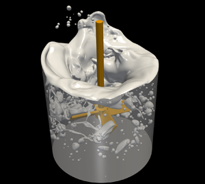
4.4 Bubbly mixing
After the brief discussion of the mechanisms underlying aeration mixing, we now increase the impeller rotation frequency to  $f=11$ Hz ( $Re=27\,500$ and $We=209$) for which the outcome is very bubbly with a total number of air bubbles being of the order of hundreds dispersed inside the water phase. We have performed this calculation using both the DNS and LES approaches and simulations with the former exhibit interesting phenomena such as the bursting effect with the main interface. Figure 9 shows the spatio-temporal evolution of the flow, using DNS, where it is seen that the initially flat interface undergoes a rapid deflection (see figure 9a–c) towards the impeller blades (see figure 9e–f) with some interfacial pinchoff without significant ligament formation and breakup (see figure 9g–h).

Figure 9. Spatio-temporal evolution for bubbly mixing with  $f\,{=}\,1/T\,{=}\,11$ Hz, $Re\,{=}\,27\,500$ and $We=209$.
At  $t=4.25\times T$, four air ligaments are formed, which grow quickly in the radial direction and break up into many bubbles (see figure 9i,j). The resulting air-ligaments forming behind each blade are not as thin as in the case described for $f=10$ Hz (see figure 8). As highlighted through figure 9(j,k), thick shaped air ligaments will breakup and disperse all around the liquid water phase. This process continues and produces a myriad of multiscale air-bubbles. Some of these bubbles have the shape of elongated thin air ligaments, also dispersed in the water phase, and eventually breakup later into smaller bubbles.
The flow is also accompanied by a series of coalescence events that occur between bubbles inside the water phase as well as with the main top interface. Small bubbles usually remain in the water phase but larger bubbles, due to buoyancy, rise to the top. When any bubble reaches the main top interface, it bursts and sometimes ejects some liquid-droplets above the interface (see figure 9n,o).
In figure 10, we have isolated several ‘singular’ events that involve topological transitions occurring in this type of bubbly mixing. Figure 10(a) highlights a coalescence event between a small bubble and the main interface. These snapshots in figure 10(a) are given at the following times, from top to bottom,  $t/T=5.92$, $5.94$ and $5.96$, respectively. We can notice that the small bubble coalesces with the vertical part of the main interface that surrounds the impeller shaft. In figure 10(b), we have also isolated the breakup event of a ligament. We can notice a rapid coalescence of a tiny bubble with this ligament before experiencing two interfacial breakups later.

Figure 10. Flow snapshots for  $f=1/T=11$ Hz, $Re=27\,500$ and $We=209$ showing bubble–interface coalescence, ligament breakup and bubble bursting through the interface in panels (a–c), respectively.
Figure 10(c) shows the temporal evolution of a bubble bursting through the main top interface, generating liquid ligaments above this interface and finally breaking up into a multitude of droplets that will fall back to the liquid bulk later on. In contrast to the coalescence described in figure 10(a), when a bubble hits the top interface, it bursts. However, if a bubble hits the vertical part of the main interface, the outcome corresponds to a simple coalescence process. Furthermore, for the latest snapshot of figure 10(c), we count a total of  $503$ bubbles dispersed inside the bulk of the water phase and also a total $33$ water drops. Some of the water drops are located above the main top interface (see the latest snapshots in figure 10c), but some others are encapsulated within some large bubbles inside the bulk water phase.
At this stage of the mixing process, it is interesting to follow the temporal evolution of the bubble sizes during the aeration process. We can notice through figure 9 that the appearance of bubbles in the liquid bulk starts at time  $t/T\approx 4.5$ (see figure 9g). Moreover, the flow can be considered as ‘bubbly’ only at $t/T\approx 5.5$ (figure 9k). It is possible to isolate all $n$ bubbles dispersed within the water phase, calculate the volume of each individual bubble $\mathcal {V}_{b,i} (i=1,n)$ and deduce an approximation of its diameter $d_{b,i}=(6\mathcal {V}_{b,i}/{\rm \pi} )^{(1/3)}$. Figure 11(a) represents the probability density function of bubble size distribution for $t/T = 10$ using both LES and DNS formulations. Most of the bubble sizes are smaller than the average value $d_{bm}$. The probability density functions are quasi-similar (see figure 11a).

Figure 11. (a) Probability density function histogram of bubble size inside the liquid bulk, normalised by the average bubble diameter,  $d_{bm}$, associated with the time $t/T=10$; (b) temporal evolution of the gas holdup $\varepsilon (t)$ generated using the DNS and LES approaches. The rest of the parameter values are the same as those used to generate figure 7.
Finally, from an engineering perspective, it is crucial to estimate the air bubble volume dispersed inside the water phase. As mentioned in the introduction, for some applications, bubbles are desirable and for others, their presence must be avoided. However, if these air bubbles are produced during a mixing process, it is important to estimate the temporal evolution of the gas holdup,  $\varepsilon$:
 \begin{equation} \varepsilon(t) = \mathcal{V}_{b}/\left(\mathcal{V}_b + \mathcal{V}_{l}\right), \end{equation}
which is the ratio of the volume of the air phase entrained within the water,  $\mathcal {V}_b=\sum _{i=1}^n \mathcal {V}_{b,i}$, to the total volume of air and water within the stirred vessel; $\mathcal {V}_l = {\rm \pi}D_b^2 h/4$ is the volume of the water phase. In figure 11(b), we show the evolution of the gas holdup $\varepsilon (t)$ highlighting its maximum value at $t/T \approx 6.25\unicode{x2013}6.5$ beyond which the dynamic equilibrium amongst bubble formation, coalescence and breakup leads to a steady $\varepsilon$. Inspection of figure 11(b) reveals that the bubbly steady-state using both DNS and LES is reached for $t/T\ge 8$ with approximately $1.9\,\%$ of air dispersed in the water bulk. The difference between these approaches is in the interval $t/T \approx 5.5\unicode{x2013}8.0$, where DNS predicts more bubbles compared to LES.
5. Conclusion and perspectives
In this paper, we have studied numerically the complex dynamics occurring during air–liquid mixing using a pitched blade turbine. The motion of the impeller and the fluid–structure interaction is computed by a direct forcing method within a general solver for multiphase flows (Reference Shin, Chergui and JuricShin et al., 2017). We have shown that vortical structures are similar for any frequency below the aeration limit. These vortical structures correspond to Kelvin–Helmholtz, blade tip, end wall and wall breakdown vortices. Aeration occurs for a sufficiently large rotational frequency, and we highlight the importance of the initial state (from rest or from an already developed flow). Future research avenues for study are to investigate further the physics of the aeration (for frequencies larger than 10 Hz) and to generalise this study through variation of the initial liquid height, the clearance and the diameter ratio between the impeller and the cylindrical tank. Another type of multiphase mixing process that has not been studied here and occurs for high frequencies,  $f\ge 15$ Hz, is ‘air envelopment’ mixing. At very high rotation frequencies, the air phase will envelop the entire impeller during the rotation. Similarly, a major route of research in turbulent mixing systems focuses on emulsification processes (liquid–liquid flows), specifically on expanding the understanding of the hydrodynamic phenomena which are similar to those studied here but in the context of liquid–liquid systems, including droplet breakage under turbulent conditions beyond the well-known Kolmogorov–Hinze theory (Reference HakanssonHakansson, 2019). Finally, industrially relevant flow systems involving fluids with complex rheological behaviour, and variable surface tension due to the presence of surfactants, could also be modelled in the future too, since the recent paper of Reference Shin, Chergui, Juric, Kahouadji, Matar and CrasterShin et al. (2018) has paved the way towards a numerical method which can handle such scenarios.
Supplementary movies
Supplementary movies are available at https://doi.org/10.1017/flo.2022.24.
Acknowledgements
D.J. and J.C. acknowledge support through HPC/AI computing time at the Institut du Développement et des Ressources en Informatique Scientifique (IDRIS) of the Centre National de la Recherche Scientifique (CNRS), coordinated by GENCI (Grand Equipement National de Calcul Intensif) Grant 2022 A0122B06721. L.K. acknowledges with gratitude P. Dossin, H. Hu and Z. Alam for the warm hospitality at Procter and Gamble where this study has been initiated. O.K.M. also acknowledges funding from PETRONAS and the Royal Academy of Engineering for a Research Chair in Multiphase Fluid Dynamics, and the PETRONAS Centre for Engineering of Multiphase Systems. Simulations have been performed using code BLUE (Reference Shin, Chergui and JuricShin et al., 2017) and the visualisations have been generated using Paraview.
Funding Statement
This work is supported by the Engineering and Physical Sciences Research Council, United Kingdom, through the MEMPHIS (EP/K003976/1) and PREMIERE (EP/T000414/1) Programme Grants, and by computing time at HPC facilities provided by the Research Computing Service (RCS) of Imperial College London.
Declaration of Interests
The authors declare no conflict of interest.
Author Contributions
All authors have contributed equally to this paper.
Data Availability Statement
Raw data are available from the corresponding author L.K.
Ethical Standards
The research meets all ethical guidelines, including adherence to the legal requirements of the study country.


 Open access