


1 Introduction
Beltrami fields, that is, eigenfunctions of the curl operator satisfying
 $$ \begin{align} \operatorname{\mathrm{curl}} u =\lambda u \end{align} $$
on ${\mathbb {R}}^3$
or on the flat torus
${\mathbb {R}}^3$
or on the flat torus ${\mathbb {T}}^3$
for some nonzero constant
${\mathbb {T}}^3$
for some nonzero constant $\lambda $
, are a classical family of stationary solutions to the Euler equation in three dimensions. However, the significance of Beltrami fields in the context of ideal fluids in equilibrium was only unveiled by V.I. Arnold in his influential work on stationary Euler flows. Indeed, Arnold’s structure theorem [Reference Arnold1, Reference Arnold2] ensures that, under suitable technical assumptions, a smooth stationary solution to the three-dimensional Euler equation is either integrable or a Beltrami field. In the language of fluid mechanics, an integrable flow is usually called laminar, so complex dynamics (as expected in Lagrangian turbulence) can only appear in a fluid in equilibrium through Beltrami fields. This connection between Lagrangian turbulence and Beltrami fields is so direct that physicists have even coined the term ‘Beltramization’ to describe the experimentally observed phenomenon that the velocity field and its curl (i.e., the vorticity) tend to align in turbulent regions (see, e.g., [Reference Farge, Pellegrino and Schneider17, Reference Monchaux, Ravelet, Dubrulle, Chiffaudel and Daviaud28]).
$\lambda $
, are a classical family of stationary solutions to the Euler equation in three dimensions. However, the significance of Beltrami fields in the context of ideal fluids in equilibrium was only unveiled by V.I. Arnold in his influential work on stationary Euler flows. Indeed, Arnold’s structure theorem [Reference Arnold1, Reference Arnold2] ensures that, under suitable technical assumptions, a smooth stationary solution to the three-dimensional Euler equation is either integrable or a Beltrami field. In the language of fluid mechanics, an integrable flow is usually called laminar, so complex dynamics (as expected in Lagrangian turbulence) can only appear in a fluid in equilibrium through Beltrami fields. This connection between Lagrangian turbulence and Beltrami fields is so direct that physicists have even coined the term ‘Beltramization’ to describe the experimentally observed phenomenon that the velocity field and its curl (i.e., the vorticity) tend to align in turbulent regions (see, e.g., [Reference Farge, Pellegrino and Schneider17, Reference Monchaux, Ravelet, Dubrulle, Chiffaudel and Daviaud28]).
Motivated by Hénon’s numerical studies of Arnold–Beltrami–Childress (ABC) flows [Reference Hénon23], which are the easiest examples of Beltrami fields, Arnold suggested [Reference Arnold1, Reference Arnold2] that Beltrami fields exhibit the same complexity as the restriction to an energy level of a typical mechanical system with two degrees of freedom. To put it differently, a typical Beltrami field should then exhibit chaotic regions coexisting with a positive measure set of invariant tori of complicated topology.
Although specific instances of chaotic ABC flows in the nearly integrable regime have been known for a long time [Reference Zhao, Kwek, Li and Huang35], Arnold’s speculation has been wide open up until recently. A major step towards the proof of this claim was the construction of Beltrami fields on ${\mathbb {R}}^3$
with periodic orbits and invariant tori (possibly with homoclinic intersections [Reference Enciso, Luque and Peralta-Salas11] inside) of arbitrary knotted topology [Reference Enciso and Peralta-Salas13, Reference Enciso and Peralta-Salas14]. In fluid mechanics, these periodic orbits and invariant tori are usually called vortex lines and vortex tubes, respectively, and in fact the existence of vortex lines of any topology had also been suggested by Arnold in the same papers. These results also hold [Reference Enciso, Peralta-Salas and Torres de Lizaur16] in the case of Beltrami fields on
${\mathbb {R}}^3$
with periodic orbits and invariant tori (possibly with homoclinic intersections [Reference Enciso, Luque and Peralta-Salas11] inside) of arbitrary knotted topology [Reference Enciso and Peralta-Salas13, Reference Enciso and Peralta-Salas14]. In fluid mechanics, these periodic orbits and invariant tori are usually called vortex lines and vortex tubes, respectively, and in fact the existence of vortex lines of any topology had also been suggested by Arnold in the same papers. These results also hold [Reference Enciso, Peralta-Salas and Torres de Lizaur16] in the case of Beltrami fields on ${\mathbb {T}}^3$
, which, contrary to what happens in the case of
${\mathbb {T}}^3$
, which, contrary to what happens in the case of ${\mathbb {R}}^3$
, have finite energy; this is important for applications because
${\mathbb {R}}^3$
, have finite energy; this is important for applications because ${\mathbb {R}}^3$
and
${\mathbb {R}}^3$
and ${\mathbb {T}}^3$
are the two main settings in which mathematical fluid mechanics is studied. The main drawback of the approach we developed to prove these results is that, while we managed to construct structurally stable Beltrami fields exhibiting complex behavior, the method of proof provides no information whatsoever about to what extent complex behavior is typical for Beltrami fields.
${\mathbb {T}}^3$
are the two main settings in which mathematical fluid mechanics is studied. The main drawback of the approach we developed to prove these results is that, while we managed to construct structurally stable Beltrami fields exhibiting complex behavior, the method of proof provides no information whatsoever about to what extent complex behavior is typical for Beltrami fields.
Our objective in this paper is to establish a probabilistic version of Arnold’s view of complexity in Beltrami fields. To do so, the key new tool is a theory of random Beltrami fields, which we develop here in order to estimate the probability that a Beltrami field exhibits certain complex dynamics. The blueprint for this is the Nazarov–Sodin theory for Gaussian random monochromatic waves, which yields asymptotic laws for the number of connected nodal components of the wave. Heuristically, the basic idea is that a Beltrami field satisfying equation (1.1) can be thought of as a vector-valued monochromatic wave; however, the vector-valued nature of the solutions and the fact that we aim to control much more sophisticated geometric objects introduces essential new difficulties from the very beginning.
1.1 Overview of the Nazarov–Sodin theory for Gaussian random monochromatic waves
The Nazarov–Sodin theory [Reference Nazarov and Sodin30], whose original motivation was to understand the nodal set of random spherical harmonics of large order [Reference Nazarov and Sodin29], provides a very efficient tool to derive asymptotic laws for the distribution of the zero set of smooth Gaussian functions of several variables. The primary examples are various Gaussian ensembles of large-degree polynomials on the sphere or on the torus and the restriction to large balls of translation-invariant Gaussian functions on ${\mathbb {R}}^d$
. Most useful for our purposes are their asymptotic results for Gaussian random monochromatic waves, which are random solutions to the Helmholtz equation
${\mathbb {R}}^d$
. Most useful for our purposes are their asymptotic results for Gaussian random monochromatic waves, which are random solutions to the Helmholtz equation
 $$ \begin{align} {\Delta} F + F=0 \end{align} $$
on ${\mathbb {R}}^d$
. We will henceforth restrict ourselves to the case
${\mathbb {R}}^d$
. We will henceforth restrict ourselves to the case $d=3$
for the sake of concreteness.
$d=3$
for the sake of concreteness.
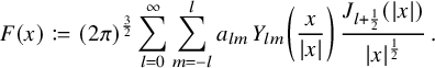
As the Fourier transform of a solution to the Helmholtz equation (1.2) must be supported on the sphere of radius 1, the way one constructs random monochromatic waves is the following [Reference Canzani and Sarnak8]. One starts with a real-valued orthonormal basis of the space of square-integrable functions on the unit two-dimensional sphere ${\mathbb {S}}$
. Although the choice of basis is immaterial, for concreteness we can think of the basis of spherical harmonics, which we denote by
${\mathbb {S}}$
. Although the choice of basis is immaterial, for concreteness we can think of the basis of spherical harmonics, which we denote by $Y_{lm}$
. Hence,
$Y_{lm}$
. Hence, $Y_{lm}$
is an eigenfunction of the spherical Laplacian with eigenvalue
$Y_{lm}$
is an eigenfunction of the spherical Laplacian with eigenvalue $l(l+1)$
, the index l is a nonnegative integer and m ranges from
$l(l+1)$
, the index l is a nonnegative integer and m ranges from $-l$
to l. The degeneracy of the eigenvalue
$-l$
to l. The degeneracy of the eigenvalue $l(l+1)$
is therefore
$l(l+1)$
is therefore $2l+1$
. To consider a Gaussian random monochromatic wave, one now sets
$2l+1$
. To consider a Gaussian random monochromatic wave, one now sets

on the unit sphere $|\xi |=1$
,
$|\xi |=1$
, $\xi \in {\mathbb {R}}^3$
, where
$\xi \in {\mathbb {R}}^3$
, where $a_{l m}$
are independent standard Gaussian random variables. One then defines F as the Fourier transform of the measure
$a_{l m}$
are independent standard Gaussian random variables. One then defines F as the Fourier transform of the measure $\varphi \, d\sigma $
, where
$\varphi \, d\sigma $
, where $d\sigma $
is the area measure of the unit sphere. This is tantamount to setting
$d\sigma $
is the area measure of the unit sphere. This is tantamount to setting
The central known result concerning the asymptotic distribution of the nodal components of Gaussian random monochromatic waves is that, almost surely, the number of connected components of the nodal set that are contained in a large ball (and even those of any fixed compact topology) grows asymptotically like the volume of the ball. More precisely, let us denote by $N_F(R)$
(respectively,
$N_F(R)$
(respectively, $N_F(R;[{\Sigma }])$
) the number of connected components of the nodal set
$N_F(R;[{\Sigma }])$
) the number of connected components of the nodal set $F^{-1}(0)$
that are contained in the ball centered at the origin of radius R (respectively, and diffeomorphic to
$F^{-1}(0)$
that are contained in the ball centered at the origin of radius R (respectively, and diffeomorphic to ${\Sigma }$
). Here,
${\Sigma }$
). Here, ${\Sigma }$
is any smooth, closed, orientable surface
${\Sigma }$
is any smooth, closed, orientable surface ${\Sigma }\subset {\mathbb {R}}^3$
. It is obvious from the definition that
${\Sigma }\subset {\mathbb {R}}^3$
. It is obvious from the definition that $N_F(R;[{\Sigma }])$
only depends on the diffeomorphism class of the surface,
$N_F(R;[{\Sigma }])$
only depends on the diffeomorphism class of the surface, $[{\Sigma }]$
. The main result of the theory—which is due to Nazarov and Sodin [Reference Nazarov and Sodin30] in the case of nodal sets of any topology, and to Sarnak and Wigman when the topology of the nodal sets is controlled [Reference Sarnak and Wigman32]— can then be stated as follows. Here and in what follows, the symbol
$[{\Sigma }]$
. The main result of the theory—which is due to Nazarov and Sodin [Reference Nazarov and Sodin30] in the case of nodal sets of any topology, and to Sarnak and Wigman when the topology of the nodal sets is controlled [Reference Sarnak and Wigman32]— can then be stated as follows. Here and in what follows, the symbol ${\xrightarrow [\mathrm {a.s.}]{L^1}}$
will be used to denote that a certain sequence of random variables converges both almost surely and in mean. Morally speaking, this is a law of large numbers for the number of connected components associated with the Gaussian field F.
${\xrightarrow [\mathrm {a.s.}]{L^1}}$
will be used to denote that a certain sequence of random variables converges both almost surely and in mean. Morally speaking, this is a law of large numbers for the number of connected components associated with the Gaussian field F.
Theorem 1.1. Let F be a monochromatic random wave. Then there are positive constants $\nu $
,
$\nu $
, $\nu ([{\Sigma }])$
such that, as
$\nu ([{\Sigma }])$
such that, as $R\to \infty $
,
$R\to \infty $
,
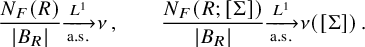 $$\begin{align*}\frac{N_F(R)}{|B_R|}{\xrightarrow[\mathrm{a.s.}]{L^1}} \nu\,,\qquad \frac{N_F(R;[{\Sigma}])}{|B_R|}{\xrightarrow[\mathrm{a.s.}]{L^1}} \nu([{\Sigma}])\,. \end{align*}$$
Here, ${\Sigma }\subset {\mathbb {R}}^3$
is any compact surface as above.
${\Sigma }\subset {\mathbb {R}}^3$
is any compact surface as above.
1.2 Gaussian random Beltrami fields on ${\mathbb {R}}^3$

Our goal is then to obtain an extension of the Nazarov–Sodin theory that applies to random Beltrami fields. As we will discuss later in the introduction, this is far from trivial because there are essential new difficulties that make the analysis of the problem rather involved.
The origin of many of these difficulties is strongly geometric. In contrast to the case of random monochromatic waves (or any other scalar Gaussian field), where the main geometric objects of interest are the components of its nodal set, in the study of random vector fields we aim to understand structures of a much subtler geometric nature. Among these structures, and in increasing order of complexity, one should certainly consider the following:
-
(i) Zeros, that is, points where the vector field vanishes.
-
(ii) Periodic orbits, which can be knotted in complicated ways.
-
(iii) Invariant tori, that is, surfaces diffeomorphic to a 2-torus that are invariant under the flow of the field. They can be knotted too.
-
(iv) Compact chaotic invariant sets, which exhibit horseshoe-type dynamics and have, in particular, positive topological entropy.
Recall that a horseshoe is defined as a compact hyperbolic invariant set with a Cantor transverse section on which the time-T flow of u is topologically conjugate to a Bernoulli shift [Reference Guckenheimer and Holmes22], for some T. Consequently, let us define the following quantities:
-
(i)
${N^{\mathrm {z}}_u}(R)$
denotes the number of zeros of u contained in the ball
$B_R$
. -
(ii) Given a (possibly knotted) closed curve
$\gamma \subset {\mathbb {R}}^3$
,
${N^{\mathrm {o}}_u}(R;[\gamma ])$
denotes the number of periodic orbits of u contained in
$B_R$
that are isotopic to
$\gamma $
. -
(iii) Given a (possibly knotted) torus
${\mathcal T}\subset {\mathbb {R}}^3$
,
${V^{\mathrm {t}}_u}(R;[{\mathcal T}])$
is the volume (understood as the inner measure) of the set of ergodic invariant tori of u that are contained in
$B_R$
and are isotopic to
${\mathcal T}$
. Ergodic means that we consider invariant tori on which the orbits of u are dense. -
(iv)
${N^{\mathrm {h}}_u}(R)$
denotes the number of horseshoes of u contained in the ball
$B_R$
.


Clearly, these quantities only depend on the isotopy class of $\gamma $
and
$\gamma $
and ${\mathcal T}$
.
${\mathcal T}$
.
It is not hard to believe that these geometric subtleties give rise to a number of analytic difficulties. One should mention, however, that there also appear other unexpected analytic difficulties whose origin is less obvious. They are related to the fact that it is not clear how to define a random Beltrami field through an analog of equation (1.3b). This is because the characterization of a monochromatic wave as the Fourier transform of a distribution supported on a sphere is the conceptual base of the simple definition (1.3a), which underlies the equivalent but considerably more awkward expression (1.3b). Heuristically, analytic difficulties stem from the fact that there is not such a clean formula in Fourier space for a general Beltrami field. This is because the three components of the Beltrami field (which are monochromatic waves) are not independent, so the reduction to a Fourier formulation with independent variables is not trivial. We refer the reader to Section 3, where we explain in detail how to define Gaussian random Beltrami fields in a way that is strongly reminiscent of equation (1.3b). Later in this introduction, we shall also informally discuss the aforementioned difficulties and discuss how we manage to circumvent them using a combination of ideas from partial differential equations, dynamical systems and probability.
We can now state our main result for Gaussian random Beltrami fields on ${\mathbb {R}}^3$
, as defined in Section 3. Let us emphasize that the picture that emerges from this theorem is fully consistent with Arnold’s view of complexity in Beltrami fields; with probability 1, we show that a random Beltrami field is ‘partially integrable’ in that there is a large volume of invariant tori, and simultaneously features many compact chaotic invariant sets and periodic orbits of arbitrarily complex topologies. This coexistence of chaos and order is indeed the essential feature of the restriction to an energy hypersurface of a generic Hamiltonian system with two degrees of freedom, as Arnold put it. In this direction, Corollary 1.3 below is quite illustrative.
${\mathbb {R}}^3$
, as defined in Section 3. Let us emphasize that the picture that emerges from this theorem is fully consistent with Arnold’s view of complexity in Beltrami fields; with probability 1, we show that a random Beltrami field is ‘partially integrable’ in that there is a large volume of invariant tori, and simultaneously features many compact chaotic invariant sets and periodic orbits of arbitrarily complex topologies. This coexistence of chaos and order is indeed the essential feature of the restriction to an energy hypersurface of a generic Hamiltonian system with two degrees of freedom, as Arnold put it. In this direction, Corollary 1.3 below is quite illustrative.
Theorem 1.2. Let u be a Gaussian random Beltrami field. Then:
-
(i) The topological entropy of u is positive almost surely. In fact, with probability
$1$
,
$$\begin{align*}\liminf_{R\to\infty} \frac{{N^{\mathrm{h}}_u}(R)}{|B_R|}>{\nu^{\mathrm{h}}}\,. \end{align*}$$
-
(ii) With probability
$1$
, the volume of ergodic invariant tori of u isotopic to a given embedded torus
${\mathcal T}\subset {\mathbb {R}}^3$
and the number of periodic orbits of u isotopic to a given closed curve
$\gamma \subset {\mathbb {R}}^3$
satisfy the volumetric growth estimate
$$\begin{align*}\liminf_{R\to\infty} \frac{{V^{\mathrm{t}}_u}(R;[{\mathcal T}])}{|B_R|}>{\nu^{\mathrm{t}}}([{\mathcal T}])\,,\qquad \liminf_{R\to\infty} \frac{{N^{\mathrm{o}}_u}(R;[\gamma])}{|B_R|}>{\nu^{\mathrm{o}}}([\gamma])\,. \end{align*}$$


The constants ${\nu ^{\mathrm {h}}}$
,
${\nu ^{\mathrm {h}}}$
, ${\nu ^{\mathrm {t}}}([{\mathcal T}])$
and
${\nu ^{\mathrm {t}}}([{\mathcal T}])$
and ${\nu ^{\mathrm {o}}}([\gamma ])$
above are all positive, for any choice of the curve
${\nu ^{\mathrm {o}}}([\gamma ])$
above are all positive, for any choice of the curve $\gamma $
and the torus
$\gamma $
and the torus ${\mathcal T}$
.
${\mathcal T}$
.
Corollary 1.3. With probability $1$
, a Gaussian random Beltrami field on
$1$
, a Gaussian random Beltrami field on ${\mathbb {R}}^3$
exhibits infinitely many horseshoes coexisting with an infinite volume of ergodic invariant tori of each isotopy type. Moreover, the set of periodic orbits contains all knot types.
${\mathbb {R}}^3$
exhibits infinitely many horseshoes coexisting with an infinite volume of ergodic invariant tori of each isotopy type. Moreover, the set of periodic orbits contains all knot types.
Remark 1.4. The result we prove (see Theorem 6.2) is in fact considerably stronger: We do not only prescribe the topology of the periodic orbits and the invariant tori we count but also other important dynamical quantities. Specifically, in the case of periodic orbits we have control over the periods (which we can pick in a certain interval $(T_1,T_2)$
) and the maximal Lyapunov exponents (which we can also pick in an interval
$(T_1,T_2)$
) and the maximal Lyapunov exponents (which we can also pick in an interval $(\Lambda _1,\Lambda _2)$
). In the case of the ergodic invariant tori, we can control the associated arithmetic and nondegeneracy conditions. Details are provided in Section 6.
$(\Lambda _1,\Lambda _2)$
). In the case of the ergodic invariant tori, we can control the associated arithmetic and nondegeneracy conditions. Details are provided in Section 6.
Unlike the case of nodal set components considered in the context of the Nazarov–Sodin theory for Gaussian random monochromatic waves, we do not prove exact asymptotics for the quantities we study but only nontrivial lower bounds that hold almost surely. Without getting technicalities at this stage, let us point out that this is related to analytic difficulties arising from the fact that we are dealing with quantities that are rather geometrically nontrivial. If one considers a simpler quantity such as the number of zeros of a Gaussian random Beltrami field, one can obtain an asymptotic distribution law similar to that of the nodal components of a random monochromatic wave, whose corresponding asymptotic constant can even be computed explicitly.
Theorem 1.5. With probability $1$
, the number of zeros of a Gaussian random Beltrami field satisfies
$1$
, the number of zeros of a Gaussian random Beltrami field satisfies
 $$\begin{align*}\frac{{N^{\mathrm{z}}_u}(R)}{|B_R|}{\xrightarrow[\mathrm{a.s.}]{L^1}} {\nu^{\mathrm{z}}} \end{align*}$$
as $R\to \infty $
. The constant is explicitly given by
$R\to \infty $
. The constant is explicitly given by
 $$ \begin{align} {\nu^{\mathrm{z}}}:= {c^{\mathrm{z}}}\int_{{\mathbb{R}}^5}|Q(z)|\, e^{-\widetilde Q(z))}\,dz=0.00872538\dots\,, \end{align} $$
where ${c^{\mathrm {z}}}:= {21^{5/2}}/[{143\sqrt 5\,\pi ^4}]$
, and
${c^{\mathrm {z}}}:= {21^{5/2}}/[{143\sqrt 5\,\pi ^4}]$
, and $Q,\widetilde Q$
are the following homogeneous polynomials in five variables:
$Q,\widetilde Q$
are the following homogeneous polynomials in five variables:
 $$ \begin{align} Q(z)&:= z_1z_2^2+z_2^3-z_1^2z_4-z_1z_2z_4-z_3^2z_4+2z_2z_3z_5-z_1z_5^2\,,\end{align} $$
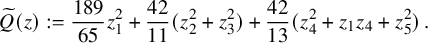 $$\begin{align}\widetilde Q(z) &:= \frac{189}{65} z_1^2+\frac{42}{11}(z_2^2+z_3^2)+\frac{42}{13}(z_4^2+z_1z_4+z_5^2)\,.\end{align} $$
1.3 Random Beltrami fields on the torus
A Beltrami field on the flat 3-torus ${\mathbb {T}}^3:=({\mathbb {R}}/2\pi \mathbb Z)^3$
(or, equivalently, on the cube of
${\mathbb {T}}^3:=({\mathbb {R}}/2\pi \mathbb Z)^3$
(or, equivalently, on the cube of ${\mathbb {R}}^3$
of side length
${\mathbb {R}}^3$
of side length $2\pi $
with periodic boundary conditions) is a vector field on
$2\pi $
with periodic boundary conditions) is a vector field on ${\mathbb {T}}^3$
satisfying the eigenvalue equation
${\mathbb {T}}^3$
satisfying the eigenvalue equation
 $$\begin{align*}\operatorname{\mathrm{curl}} v= \lambda v \end{align*}$$
for some real number $\lambda \neq 0$
. It is well known (see, e.g., [Reference Enciso, Lucà and Peralta-Salas10]) that the spectrum of the curl operator on the
$\lambda \neq 0$
. It is well known (see, e.g., [Reference Enciso, Lucà and Peralta-Salas10]) that the spectrum of the curl operator on the $3$
-torus consists of the numbers of the form
$3$
-torus consists of the numbers of the form $\lambda =\pm |k|$
for some vector with integer coefficients
$\lambda =\pm |k|$
for some vector with integer coefficients $k\in \mathbb Z^3$
. Restricting our attention to the case of positive eigenvalues for the sake of concreteness, one can therefore label the eigenvalue by a positive integer L such that
$k\in \mathbb Z^3$
. Restricting our attention to the case of positive eigenvalues for the sake of concreteness, one can therefore label the eigenvalue by a positive integer L such that $\lambda _L=L^{1/2}$
. The multiplicity of the eigenvalue is given by the cardinality of the corresponding set of spatial frequencies,
$\lambda _L=L^{1/2}$
. The multiplicity of the eigenvalue is given by the cardinality of the corresponding set of spatial frequencies,
 $$\begin{align*}{\mathcal{Z}}_L:= \{k\in\mathbb Z^3: |k|^2=L\}\,. \end{align*}$$
By Legendre’s three-square theorem, ${\mathcal {Z}}_L$
is nonempty (and therefore
${\mathcal {Z}}_L$
is nonempty (and therefore $\lambda _L$
is an eigenvalue of the curl operator) if and only if L is not of the form
$\lambda _L$
is an eigenvalue of the curl operator) if and only if L is not of the form $4^a(8b+7)$
for nonnegative integers a and b.
$4^a(8b+7)$
for nonnegative integers a and b.
The Beltrami fields corresponding to the eigenvalue $\lambda _L$
must obviously be of the form
$\lambda _L$
must obviously be of the form
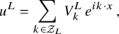 $$ \begin{align*} u^L=\sum_{k\in{\mathcal{Z}}_L} V_k^L\, e^{ik\cdot x}\,, \end{align*} $$
for some vectors $V_k^L\in {\mathbb {C}}^3$
, where
$V_k^L\in {\mathbb {C}}^3$
, where $V_k^L= \overline {V_{-k}^L}$
to ensure that the Beltrami field is real-valued. Starting from this formula, in Section 7 we define the Gaussian ensemble of random Beltrami fields
$V_k^L= \overline {V_{-k}^L}$
to ensure that the Beltrami field is real-valued. Starting from this formula, in Section 7 we define the Gaussian ensemble of random Beltrami fields $u^L$
of frequency
$u^L$
of frequency $\lambda _L$
, which we parametrize by L. The natural length scale of the problem is
$\lambda _L$
, which we parametrize by L. The natural length scale of the problem is $L^{1/2}$
.
$L^{1/2}$
.
Our objective is to study to what extent the appearance of the various dynamical objects described above (i.e., horseshoes, zeros and periodic orbits and ergodic invariant tori of prescribed topology) is typical in high-frequency Beltrami fields, which corresponds to the limit $L\to \infty $
. When taking this limit, we shall always assume that the integer L is admissible, by which we mean that it is congruent with 1, 2, 3, 5 or 6 modulo 8. We will see in Section 7 (see also [Reference Rozenshein31]) that this number-theoretic condition ensures that the dimension of the space of Beltrami fields with eigenvalue
$L\to \infty $
. When taking this limit, we shall always assume that the integer L is admissible, by which we mean that it is congruent with 1, 2, 3, 5 or 6 modulo 8. We will see in Section 7 (see also [Reference Rozenshein31]) that this number-theoretic condition ensures that the dimension of the space of Beltrami fields with eigenvalue $\lambda _L$
tends to infinity as
$\lambda _L$
tends to infinity as $L\to \infty $
.
$L\to \infty $
.
To state our main result about high-frequency random Beltrami fields in the torus, we need to introduce some notation. In parallel with the previous subsection, for any closed curve $\gamma $
and any embedded torus
$\gamma $
and any embedded torus ${\mathcal T}$
, let us respectively denote by
${\mathcal T}$
, let us respectively denote by ${N^{\mathrm {z}}_{u^L}}$
,
${N^{\mathrm {z}}_{u^L}}$
, ${N^{\mathrm {h}}_{u^L}}$
,
${N^{\mathrm {h}}_{u^L}}$
, ${N^{\mathrm {o}}_{u^L}}([\gamma ])$
and
${N^{\mathrm {o}}_{u^L}}([\gamma ])$
and ${N^{\mathrm {t}}_{u^L}}([{\mathcal T}])$
the number of zeros, horseshoes, periodic orbits isotopic to
${N^{\mathrm {t}}_{u^L}}([{\mathcal T}])$
the number of zeros, horseshoes, periodic orbits isotopic to $\gamma $
and ergodic invariant tori isotopic to
$\gamma $
and ergodic invariant tori isotopic to ${\mathcal T}$
of the field
${\mathcal T}$
of the field $u^L$
, as well as the volume (i.e., inner measure) of these tori, which we denote by
$u^L$
, as well as the volume (i.e., inner measure) of these tori, which we denote by ${V^{\mathrm {t}}_{u^L}}([{\mathcal T}])$
. To further control the distribution of these objects, let us define the number of approximately equidistributed ergodic invariant tori,
${V^{\mathrm {t}}_{u^L}}([{\mathcal T}])$
. To further control the distribution of these objects, let us define the number of approximately equidistributed ergodic invariant tori, ${N^{\mathrm {t,e}}_{u^L}}([{\mathcal T}])$
, as the largest integer m for which
${N^{\mathrm {t,e}}_{u^L}}([{\mathcal T}])$
, as the largest integer m for which $u^L$
has m ergodic invariant tori isotopic to
$u^L$
has m ergodic invariant tori isotopic to ${\mathcal T}$
that are at a distance greater than
${\mathcal T}$
that are at a distance greater than $m^{-1/3}$
apart from one another. The number of approximately equidistributed horseshoes
$m^{-1/3}$
apart from one another. The number of approximately equidistributed horseshoes $N^{\mathrm {h},\mathrm {e}}_{u^L}$
, periodic orbits isotopic to a curve
$N^{\mathrm {h},\mathrm {e}}_{u^L}$
, periodic orbits isotopic to a curve $N^{\mathrm {o},\mathrm {e}}_{u^L}([\gamma ])$
and zeros
$N^{\mathrm {o},\mathrm {e}}_{u^L}([\gamma ])$
and zeros $N^{\mathrm {z},\mathrm {e}}_{u^L}$
are defined analogously. Note that, again, the asymptotic information that we obtain is perfectly aligned with Arnold’s view of complex behavior in typical Beltrami fields.
$N^{\mathrm {z},\mathrm {e}}_{u^L}$
are defined analogously. Note that, again, the asymptotic information that we obtain is perfectly aligned with Arnold’s view of complex behavior in typical Beltrami fields.
Theorem 1.6. Let us denote by $(u^L)$
the parametric Gaussian ensemble of random Beltrami fields on
$(u^L)$
the parametric Gaussian ensemble of random Beltrami fields on ${\mathbb {T}}^3$
, where L ranges over the set of admissible integers. Consider any contractible closed curve
${\mathbb {T}}^3$
, where L ranges over the set of admissible integers. Consider any contractible closed curve $\gamma $
and any contractible embedded torus
$\gamma $
and any contractible embedded torus ${\mathcal T}$
in
${\mathcal T}$
in ${\mathbb {T}}^3$
. Then:
${\mathbb {T}}^3$
. Then:
-
(i) With a probability tending to
$1$
as
$L\to \infty $
, the field
$u^L$
exhibits an arbitrarily large number of approximately equidistributed horseshoes, zeros, periodic orbits isotopic to
$\gamma $
and ergodic invariant tori isotopic to
${\mathcal T}$
. More precisely, for any integer m,
$$\begin{align*}\lim_{L\to \infty} {\mathbb{P}}\Big\{\min\big\{N^{\mathrm{h},\mathrm{e}}_{u^L},{N^{\mathrm{t,e}}_{u^L}}([{\mathcal T}]),N^{\mathrm{o},\mathrm{e}}_{u^L}([\gamma]),N^{\mathrm{z},\mathrm{e}}_{u^L}\big\}>m\Big\}=1\,. \end{align*}$$
Furthermore, the probability that the topological entropy of the field grows at least as
$L^{1/2}$
and that there are infinitely many ergodic invariant tori of
$u^L$
isotopic to
${\mathcal T}$
also tends to
$1$
:
$$\begin{align*}\lim_{L\to \infty} {\mathbb{P}}\big\{{N^{\mathrm{t}}_{u^L}}([{\mathcal T}])=\infty\; \text{ and } \; {h_{\mathrm{top}}}(u^L)> {\nu^{\mathrm{h}}_*} L^{1/2}\big\}=1\,. \end{align*}$$
-
(ii) The expected volume of the ergodic invariant tori of
$u^L$
isotopic to
${\mathcal T}$
is uniformly bounded from below, and the expected number of horseshoes and periodic orbits isotopic to
$\gamma $
is at least of order
$L^{3/2}$
:
$$ \begin{align*} \liminf_{L\to\infty} \min\Bigg\{\frac{{\mathbb{E}}{N^{\mathrm{h}}_{u^L}}}{L^{3/2}}\,, \frac{{\mathbb{E}}{N^{\mathrm{o}}_{u^L}}([\gamma])}{L^{3/2}}\,, {\mathbb{E}} {V^{\mathrm{t}}_{u^L}}([{\mathcal T}])\Bigg\}>\nu_*([\gamma],[{\mathcal T}])\,. \end{align*} $$
In the case of zeros, the asymptotic expectation is explicit, with
${\nu ^{\mathrm {z}}}$
given by (1.4):
$$\begin{align*}\lim_{L\to\infty}\frac{{\mathbb{E}}{N^{\mathrm{z}}_{u^L}}}{L^{3/2}}= (2\pi)^3{\nu^{\mathrm{z}}}\,. \end{align*}$$


Here, ${\nu ^{\mathrm {h}}_*}$
and
${\nu ^{\mathrm {h}}_*}$
and $\nu _*([\gamma ],[{\mathcal T}])$
are positive constants.
$\nu _*([\gamma ],[{\mathcal T}])$
are positive constants.
Remark 1.7. As in the case of ${\mathbb {R}}^3$
, the result we prove in Section 7 is actually stronger in the sense that we have control over important dynamical quantities (which now depend strongly on L) describing the flow near the above invariant tori and periodic orbits.
${\mathbb {R}}^3$
, the result we prove in Section 7 is actually stronger in the sense that we have control over important dynamical quantities (which now depend strongly on L) describing the flow near the above invariant tori and periodic orbits.
1.4 Some technical remarks
In a way, the cornerstone of the Nazarov–Sodin theory is their very clever (and non-probabilistic) ‘sandwich estimate’, which relates the number $N_F(R)$
of connected components of the nodal set of the Gaussian random field F that are contained in an arbitrarily large ball
$N_F(R)$
of connected components of the nodal set of the Gaussian random field F that are contained in an arbitrarily large ball $B_R$
with ergodic averages of the same quantity involving the number of components contained in balls of fixed radius. Two ingredients are key to effectively apply this sandwich estimate. On the one hand, each nodal component cannot be too small by the Faber–Krahn inequality, which ensures, in dimension 3, that its volume is at least
$B_R$
with ergodic averages of the same quantity involving the number of components contained in balls of fixed radius. Two ingredients are key to effectively apply this sandwich estimate. On the one hand, each nodal component cannot be too small by the Faber–Krahn inequality, which ensures, in dimension 3, that its volume is at least $c\lambda ^{-3}$
if
$c\lambda ^{-3}$
if ${\Delta } F+\lambda ^2F=0$
. On the other hand, to control the connected components that intersect a large ball but are not contained in it, it suffices to employ the Kac–Rice formula to derive bounds for the number of critical points of a certain family of Gaussian random functions.
${\Delta } F+\lambda ^2F=0$
. On the other hand, to control the connected components that intersect a large ball but are not contained in it, it suffices to employ the Kac–Rice formula to derive bounds for the number of critical points of a certain family of Gaussian random functions.
In the setting of random Beltrami fields, the need for new ideas becomes apparent the moment one realizes that there are no reasonable substitutes for these two key ingredients. That is, the frequency $\lambda $
does not provide bounds for the size of the more sophisticated geometric objects considered in this context (i.e., periodic orbits, invariant tori or horseshoes), and one cannot estimate the objects that intersect a ball but are not contained in it using a Kac–Rice formula. As a matter of fact, we have not managed to obtain any useful bounds for these quantities, and, while we do use a sandwich inequality of sorts (or at least lower bounds that can be regarded as a weaker substitute thereof), even the measurability of the various objects of interest becomes a nontrivial issue due to their complicated geometric properties.
$\lambda $
does not provide bounds for the size of the more sophisticated geometric objects considered in this context (i.e., periodic orbits, invariant tori or horseshoes), and one cannot estimate the objects that intersect a ball but are not contained in it using a Kac–Rice formula. As a matter of fact, we have not managed to obtain any useful bounds for these quantities, and, while we do use a sandwich inequality of sorts (or at least lower bounds that can be regarded as a weaker substitute thereof), even the measurability of the various objects of interest becomes a nontrivial issue due to their complicated geometric properties.
To circumvent these problems, we employ different kinds of techniques. Firstly, ideas from the theory of dynamical systems play a substantial role in our proofs. On the one hand, KAM theory and hyperbolic dynamics are important to prove that certain carefully chosen functionals are lower semicontinuous, which is key to solve measurability issues that would be very hard to deal with otherwise. Furthermore, to prove that Beltrami fields exhibit chaotic behavior almost surely, it is essential to have at least one example of a Beltrami field that features a horseshoe, and even that was not known. Indeed, the available examples of nonintegrable ABC flows are known to be chaotic on ${\mathbb {T}}^3$
due to the noncontractibility of the domain but not on
${\mathbb {T}}^3$
due to the noncontractibility of the domain but not on ${\mathbb {R}}^3$
. This technical point is fundamental and makes them unsuitable for the study of random Beltrami fields. Therefore, an important step in our proof is to construct, using Melnikov theory, a Beltrami field on
${\mathbb {R}}^3$
. This technical point is fundamental and makes them unsuitable for the study of random Beltrami fields. Therefore, an important step in our proof is to construct, using Melnikov theory, a Beltrami field on ${\mathbb {R}}^3$
that has a horseshoe. Techniques from Fourier analysis and from the global approximation theory for Beltrami fields are also necessary to handle the inherent difficulties that stem from the fact that the equation under consideration is more complicated than that of a monochromatic wave. As an aside, the only point of the paper where we use the Kac–Rice formula is to compute the constant
${\mathbb {R}}^3$
that has a horseshoe. Techniques from Fourier analysis and from the global approximation theory for Beltrami fields are also necessary to handle the inherent difficulties that stem from the fact that the equation under consideration is more complicated than that of a monochromatic wave. As an aside, the only point of the paper where we use the Kac–Rice formula is to compute the constant ${\nu ^{\mathrm {z}}}$
in closed form.
${\nu ^{\mathrm {z}}}$
in closed form.
In the case of Beltrami fields on the torus, the results we prove concern not only the expected values of the quantities of interest but also the probability of events. In the case of random monochromatic waves on the torus, Nazarov and Sodin [Reference Nazarov and Sodin30] had proved results for the expectation (which apply to very general parametric scalar Gaussian ensembles), and Rozenshein [Reference Rozenshein31] had derived very precise exponential bounds for the probability akin to those established by Nazarov and Sodin [Reference Nazarov and Sodin29] for random spherical harmonics. However, both results use in a crucial way that the size of nodal components can be effectively estimated in terms of the frequency: The Faber–Krahn inequality provides a lower bound for the volume and large diameter components can be ruled out using a Crofton-type formula and Bézout’s theorem. No such bounds hold in the case of Beltrami fields, so the way we pass from the information that the rescaled covariant kernel of $u^L$
tends to that of u to asymptotics for the distribution of invariant tori, horseshoes or periodic orbits is completely different. Specifically, we rely on a direct argument ensuring the weak convergence of sequences of probability measures, on spaces of smooth functions, provided that suitable tightness conditions are satisfied.
$u^L$
tends to that of u to asymptotics for the distribution of invariant tori, horseshoes or periodic orbits is completely different. Specifically, we rely on a direct argument ensuring the weak convergence of sequences of probability measures, on spaces of smooth functions, provided that suitable tightness conditions are satisfied.
1.5 Outline of the paper
In Section 2, we start by describing Beltrami fields in ${\mathbb {R}}^3$
from the point of view of Fourier analysis and provide some results about global approximation. Gaussian random Beltrami fields on
${\mathbb {R}}^3$
from the point of view of Fourier analysis and provide some results about global approximation. Gaussian random Beltrami fields on ${\mathbb {R}}^3$
are introduced in Section 3, where we also establish several results about the structure of the corresponding covariance matrix and about the induced probability measure on the space of smooth vector fields. In Section 4, we recall, in a form that will be useful in later sections, several previous results about ergodic invariant tori and periodic orbits arising in Beltrami fields. Section 5 is devoted to constructing a Beltrami field on
${\mathbb {R}}^3$
are introduced in Section 3, where we also establish several results about the structure of the corresponding covariance matrix and about the induced probability measure on the space of smooth vector fields. In Section 4, we recall, in a form that will be useful in later sections, several previous results about ergodic invariant tori and periodic orbits arising in Beltrami fields. Section 5 is devoted to constructing a Beltrami field on ${\mathbb {R}}^3$
that is stably chaotic. Finally, in Sections 6 and 7, we complete the proofs of our main results in the case of
${\mathbb {R}}^3$
that is stably chaotic. Finally, in Sections 6 and 7, we complete the proofs of our main results in the case of ${\mathbb {R}}^3$
and
${\mathbb {R}}^3$
and ${\mathbb {T}}^3$
, respectively. The paper concludes with an appendix where we provide a fairly complete Fourier-theoretic characterization of Beltrami fields.
${\mathbb {T}}^3$
, respectively. The paper concludes with an appendix where we provide a fairly complete Fourier-theoretic characterization of Beltrami fields.
2 Fourier analysis and approximation of Beltrami fields
In what follows, we will say that a vector field u on ${\mathbb {R}}^3$
is a Beltrami field if
${\mathbb {R}}^3$
is a Beltrami field if
 $$\begin{align*}\operatorname{\mathrm{curl}} u = u\,. \end{align*}$$
Taking the curl of this equation and using that necessarily $\operatorname {\mathrm {div}} u=0$
, it is easy to see that u must also satisfy the Helmholtz equation:
$\operatorname {\mathrm {div}} u=0$
, it is easy to see that u must also satisfy the Helmholtz equation:
 $$\begin{align*}{\Delta} u +u=0\,. \end{align*}$$
To put it differently, the components of this vector field are monochromatic waves. An immediate consequence of this is that the Fourier transform ${\widehat {u}}$
of a polynomially bounded Beltrami field is a (vector-valued) distribution supported on the unit sphere
${\widehat {u}}$
of a polynomially bounded Beltrami field is a (vector-valued) distribution supported on the unit sphere
 $$\begin{align*}{\mathbb{S}}:=\{\xi\in{\mathbb{R}}^3:|\xi|=1\}\,. \end{align*}$$
Since u is real-valued, ${\widehat {u}}$
must be Hermitian, that is,
${\widehat {u}}$
must be Hermitian, that is, ${\widehat {u}}(\xi )= \overline {{\widehat {u}}(-\xi )}$
. Furthermore, a classical result due to Herglotz [Reference Hörmander26, Theorem 7.1.28] ensures that if u is a Beltrami field with the sharp fall off at infinity, then there is a Hermitian vector-valued function
${\widehat {u}}(\xi )= \overline {{\widehat {u}}(-\xi )}$
. Furthermore, a classical result due to Herglotz [Reference Hörmander26, Theorem 7.1.28] ensures that if u is a Beltrami field with the sharp fall off at infinity, then there is a Hermitian vector-valued function $f\in L^2({\mathbb {S}},{\mathbb {C}}^3)$
such that
$f\in L^2({\mathbb {S}},{\mathbb {C}}^3)$
such that ${\widehat {u}} = f\, d{\sigma }$
; for the benefit of the reader, details on this and other related matters are summarized in Appendix A. For short, we shall simply write this relation as
${\widehat {u}} = f\, d{\sigma }$
; for the benefit of the reader, details on this and other related matters are summarized in Appendix A. For short, we shall simply write this relation as $u=U_f$
, with
$u=U_f$
, with
 $$ \begin{align} U_f(x) :=\int_{\mathbb{S}} f(\xi)\, e^{i\xi\cdot x}\, d{\sigma}(\xi)\,. \end{align} $$
Obviously, $U_f$
is a Beltrami field if and only if f is Hermitian (which makes
$U_f$
is a Beltrami field if and only if f is Hermitian (which makes $U_f$
real-valued) and if it satisfies the distributional equation on the sphere
$U_f$
real-valued) and if it satisfies the distributional equation on the sphere
 $$ \begin{align} i\xi\times f(\xi)=f(\xi)\,. \end{align} $$
In this paper, we are particularly interested in Beltrami fields of the form $u=U_f$
, where now f is a general Hermitian vector-valued distribution on the sphere. The corresponding integral, which is convergent if f is integrable, must be understood in the sense of distributions for less regular f (that is to say, for f in the scale of Sobolev spaces
$u=U_f$
, where now f is a general Hermitian vector-valued distribution on the sphere. The corresponding integral, which is convergent if f is integrable, must be understood in the sense of distributions for less regular f (that is to say, for f in the scale of Sobolev spaces $H^s({\mathbb {S}},{\mathbb {C}}^3)$
with
$H^s({\mathbb {S}},{\mathbb {C}}^3)$
with $s<0$
). We recall, in particular, that for any integer
$s<0$
). We recall, in particular, that for any integer $k\geqslant 0$
the field
$k\geqslant 0$
the field $U_f$
is bounded as [Reference Enciso, Peralta-Salas and Romaniega15, Appendix A]
$U_f$
is bounded as [Reference Enciso, Peralta-Salas and Romaniega15, Appendix A]
 $$ \begin{align} \sup_{R>0} \frac1R\int_{B_R}\frac{|U_f(x)|^2}{1+|x|^{2k}}\, dx\leqslant C\|f\|_{H^{-k}({\mathbb{S}},{\mathbb{C}}^3)}\,. \end{align} $$
We recall that, for any real s, the $H^s({\mathbb {S}})$
norm of a function f can be computed as
$H^s({\mathbb {S}})$
norm of a function f can be computed as
 $$\begin{align*}\|f\|_{H^s({\mathbb{S}})}^2=\sum_{l=0}^{\infty}\sum_{m=-l}^{l} (l+1)^{2s}|f_{l m}|^2\,, \end{align*}$$
where $f_{lm}$
are the coefficients of the spherical harmonics expansion of f.
$f_{lm}$
are the coefficients of the spherical harmonics expansion of f.
With $q(t):= \frac 18(\frac {15}{\pi })^{1/2}(1+\sqrt 7 i\, t)$
, let us consider the vector-valued polynomial
$q(t):= \frac 18(\frac {15}{\pi })^{1/2}(1+\sqrt 7 i\, t)$
, let us consider the vector-valued polynomial
 $$ \begin{align} p(\xi):=q(\xi_1)\, (\xi_1^2-1,\xi_1\xi_2-i\xi_3,\xi_1\xi_3+i\xi_2)\,, \end{align} $$
which we will regard as a Hermitian function $p:{\mathbb {R}}^3\to {\mathbb {C}}^3$
. Note that the restriction of p to the sphere vanishes exactly at the poles
$p:{\mathbb {R}}^3\to {\mathbb {C}}^3$
. Note that the restriction of p to the sphere vanishes exactly at the poles $\xi _{\pm }:=(\pm 1,0,0)$
. The inessential nonvanishing normalization factor
$\xi _{\pm }:=(\pm 1,0,0)$
. The inessential nonvanishing normalization factor $q(\xi _1)$
has been introduced for later convenience: When we define random Beltrami fields via the function p in Section 3, this choice of p will ensure that the associated covariance matrix is the identity on the diagonal (see Corollary 3.6).
$q(\xi _1)$
has been introduced for later convenience: When we define random Beltrami fields via the function p in Section 3, this choice of p will ensure that the associated covariance matrix is the identity on the diagonal (see Corollary 3.6).
We next show that, away from the poles, the density f of a Beltrami field $U_f$
must point in the same direction as p.
$U_f$
must point in the same direction as p.
Proposition 2.1. The following statements hold:
-
(i) If the vector field
$U_f$
is a Beltrami field, then
$p\times f=0$
as a distribution on
${\mathbb {S}}$
. Furthermore, if
$\chi $
is a smooth real-valued function on the sphere supported in
${\mathbb {S}}\backslash \{\xi _+,\xi _-\}$
and
$f\in H^s({\mathbb {S}},{\mathbb {C}}^3)$
for some real s, then there is a Hermitian scalar function
$\varphi \in H^s({\mathbb {S}})$
such that
$\chi \, f= \varphi \, p$
. -
(ii) Conversely, for any Hermitian
$\varphi \in H^s({\mathbb {S}})$
, the associated field
$U_{\varphi p}$
is a Beltrami field.


Proof. In view of equation (2.2), for each vector $\xi \in {\mathbb {S}}$
, consider the linear map
$\xi \in {\mathbb {S}}$
, consider the linear map $M_{\xi }$
on
$M_{\xi }$
on ${\mathbb {C}}^3$
defined as
${\mathbb {C}}^3$
defined as
 $$\begin{align*}M_{\xi} V:=V-i\xi\times V\,. \end{align*}$$
More explicitly, $M_{\xi }$
is the matrix
$M_{\xi }$
is the matrix
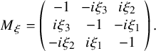 $$ \begin{align*}M_{\xi}=\left( \begin{array}{ccc} -1& -i \xi_3 & i \xi_2 \\ i \xi_3 & -1 & -i \xi_1 \\ -i \xi_2& i \xi_1 &-1 \\ \end{array} \right)\,. \end{align*} $$
The determinant of this matrix is $\det M_{\xi }=\xi _1^2+\xi _2^2+\xi _3^2-1$
, and in fact it is easy to see that
$\det M_{\xi }=\xi _1^2+\xi _2^2+\xi _3^2-1$
, and in fact it is easy to see that $M_{\xi }$
has rank 2 for any unit vector
$M_{\xi }$
has rank 2 for any unit vector $\xi $
. Since
$\xi $
. Since $M_{\xi } p(\xi )=0$
for all
$M_{\xi } p(\xi )=0$
for all $\xi \in {\mathbb {S}}$
and
$\xi \in {\mathbb {S}}$
and $p(\xi )$
only vanishes if
$p(\xi )$
only vanishes if $\xi =\xi _{\pm }$
, we then obtain that the kernel of
$\xi =\xi _{\pm }$
, we then obtain that the kernel of $M_{\xi }$
is spanned by the vector
$M_{\xi }$
is spanned by the vector $p(\xi )$
whenever
$p(\xi )$
whenever $\xi $
is not one of the poles
$\xi $
is not one of the poles $\xi _{\pm }$
. In a neighborhood of the poles, the kernel of
$\xi _{\pm }$
. In a neighborhood of the poles, the kernel of $M_{\xi }$
can be described as the linear span of
$M_{\xi }$
can be described as the linear span of $\widetilde p(\xi ):= q(\xi _2)\, (\xi _1\xi _2+i\xi _3,\xi _2^2-1, \xi _2\xi _3-i \xi _1)$
.
$\widetilde p(\xi ):= q(\xi _2)\, (\xi _1\xi _2+i\xi _3,\xi _2^2-1, \xi _2\xi _3-i \xi _1)$
.
Since $M_{\xi } f(\xi )=0$
in the sense of distributions by equation (2.2), it stems from the above analysis that one can write
$M_{\xi } f(\xi )=0$
in the sense of distributions by equation (2.2), it stems from the above analysis that one can write
 $$\begin{align*}f(\xi)= {\alpha}(\xi)\, p(\xi) \end{align*}$$
for $\xi $
away from the poles, and
$\xi $
away from the poles, and
 $$\begin{align*}f(\xi)= \beta(\xi)\, \widetilde p(\xi) \end{align*}$$
in a neighborhood of the poles; here, ${\alpha }$
and
${\alpha }$
and $\beta $
are complex-valued scalars. As
$\beta $
are complex-valued scalars. As $p(\xi )\times \widetilde p(\xi )=0$
for all
$p(\xi )\times \widetilde p(\xi )=0$
for all $\xi \in {\mathbb {S}}$
, we immediately infer that
$\xi \in {\mathbb {S}}$
, we immediately infer that
 $$\begin{align*}p\times f=0\,. \end{align*}$$
Also, as the support of a function is a closed set, p is bounded away from zero on the support of $\chi $
, so we have that
$\chi $
, so we have that
 $$\begin{align*}\varphi:= \chi \frac{f\cdot p}{|p|^2}\in H^s({\mathbb{S}})\,. \end{align*}$$
As f is Hermitian, this proves the first part of the proposition. The second statement follows immediately from the fact that
 $$\begin{align*}M_{\xi}[\varphi(\xi)p(\xi)]= \varphi(\xi)\,M_{\xi} p(\xi)=0\,. \end{align*}$$
Remark 2.2. A Beltrami field of the form $U_{\varphi p}$
can be written in terms of the scalar function
$U_{\varphi p}$
can be written in terms of the scalar function $\psi (x):= -\int _{\mathbb {S}} e^{i\xi \cdot x} q(\xi _1)\, \varphi (\xi )\, d{\sigma }(\xi )$
(which satisfies the equation
$\psi (x):= -\int _{\mathbb {S}} e^{i\xi \cdot x} q(\xi _1)\, \varphi (\xi )\, d{\sigma }(\xi )$
(which satisfies the equation ${\Delta }\psi +\psi =0$
) as
${\Delta }\psi +\psi =0$
) as
 $$\begin{align*}U_{\varphi p}=(\operatorname{\mathrm{curl}} \operatorname{\mathrm{curl}} +\operatorname{\mathrm{curl}}) (\psi,0,0)\,. \end{align*}$$
When $\varphi $
is smooth, the Beltrami field has the sharp decay bound
$\varphi $
is smooth, the Beltrami field has the sharp decay bound
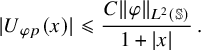 $$ \begin{align*}|U_{\varphi p}(x)|\leqslant \frac{C\|\varphi\|_{L^2({\mathbb{S}})}}{1+|x|}\,.\end{align*} $$
Remark 2.3. Not any Beltrami field of the form $U_f$
can be written as
$U_f$
can be written as $U_{\varphi p}$
for some scalar function
$U_{\varphi p}$
for some scalar function $\varphi $
: An obvious counterexample is given by
$\varphi $
: An obvious counterexample is given by
 $$ \begin{align} f(\xi):= (0,1,i)\, \delta_{\xi_+ }(\xi) + (0,1,-i) \, \delta_{\xi_- }(\xi) \,, \end{align} $$
where $\delta _{\xi _{\pm }}$
is the Dirac measure supported on the pole
$\delta _{\xi _{\pm }}$
is the Dirac measure supported on the pole $\xi _{\pm }=(\pm 1,0,0)$
. The reason for which we cannot hope to describe all Beltrami fields using just scalar multiples of a fixed complex-valued continuous vector field
$\xi _{\pm }=(\pm 1,0,0)$
. The reason for which we cannot hope to describe all Beltrami fields using just scalar multiples of a fixed complex-valued continuous vector field $p'$
is topological. Indeed, as u is divergence-free, we have that
$p'$
is topological. Indeed, as u is divergence-free, we have that $\xi \cdot p'(\xi )=0$
, so
$\xi \cdot p'(\xi )=0$
, so $p'$
must be a tangent complex-valued vector field on
$p'$
must be a tangent complex-valued vector field on ${\mathbb {S}}$
. By the hairy ball theorem, the real part of
${\mathbb {S}}$
. By the hairy ball theorem, the real part of $p'$
must then have at least one zero
$p'$
must then have at least one zero $\xi ^*$
. The equation
$\xi ^*$
. The equation $i\xi \times p'(\xi )= p'(\xi )$
implies that the imaginary part of
$i\xi \times p'(\xi )= p'(\xi )$
implies that the imaginary part of $p'$
also vanishes at
$p'$
also vanishes at $\xi ^*$
, so in fact
$\xi ^*$
, so in fact $p'(\xi ^*)=0$
. This means that densities f such as equation (2.5), where we can take
$p'(\xi ^*)=0$
. This means that densities f such as equation (2.5), where we can take $\xi ^*:= \xi _+$
without any loss of generality, cannot be written in the form
$\xi ^*:= \xi _+$
without any loss of generality, cannot be written in the form $\varphi p'$
.
$\varphi p'$
.
Intuitively speaking, Proposition 2.1 means that any Beltrami field $U_f$
whose density f is not too concentrated on
$U_f$
whose density f is not too concentrated on $\xi _{\pm }$
can be approximated globally by a field of the form
$\xi _{\pm }$
can be approximated globally by a field of the form $U_{\varphi p}$
. More precisely, one can prove the following.
$U_{\varphi p}$
. More precisely, one can prove the following.
Proposition 2.4. Consider a Hermitian vector-valued distribution f on ${\mathbb {S}}$
that satisfies the distributional equation (2.2), and define
${\mathbb {S}}$
that satisfies the distributional equation (2.2), and define
 $$\begin{align*}\varepsilon_{f,k}:= \inf \big\{\|\Theta f\|_{H^{-k}({\mathbb{S}})} : \Theta\in C^{\infty}({\mathbb{S}}),\; \Theta(\xi_+)=\Theta(\xi_-)=1\big\}\,. \end{align*}$$
If $\varepsilon _{f,k}$
is finite and
$\varepsilon _{f,k}$
is finite and $\varepsilon>\varepsilon _{f,k}$
, one can then take a Hermitian scalar distribution on the sphere
$\varepsilon>\varepsilon _{f,k}$
, one can then take a Hermitian scalar distribution on the sphere $\varphi $
, which is in fact a finite linear combination of spherical harmonics if
$\varphi $
, which is in fact a finite linear combination of spherical harmonics if $f\in H^{-k}({\mathbb {S}},{\mathbb {C}}^3)$
, such that
$f\in H^{-k}({\mathbb {S}},{\mathbb {C}}^3)$
, such that
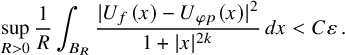 $$\begin{align*}\sup_{R>0}\frac1R\int_{B_R} \frac{|U_f(x)-U_{\varphi p}(x)|^2}{1+|x|^{2k}}\, dx< C\varepsilon\,. \end{align*}$$
Furthermore, $\varepsilon _{f,0}=0$
if
$\varepsilon _{f,0}=0$
if $f\in L^2({\mathbb {S}},{\mathbb {C}}^3)$
.
$f\in L^2({\mathbb {S}},{\mathbb {C}}^3)$
.
Proof. The first assertion is a straightforward consequence of the first part of Proposition 2.1 and of the estimate (2.3). Indeed, since f is a compactly supported distribution, then $f\in H^s({\mathbb {S}},{\mathbb {C}}^3)$
for some s. Take any
$f\in H^s({\mathbb {S}},{\mathbb {C}}^3)$
for some s. Take any $\varepsilon '\in (\varepsilon _{f,k},\varepsilon )$
, and let us consider a function
$\varepsilon '\in (\varepsilon _{f,k},\varepsilon )$
, and let us consider a function $\Theta $
as above such that
$\Theta $
as above such that $\|\Theta f\|_{H^{-k}({\mathbb {S}})} <\varepsilon '$
. Since
$\|\Theta f\|_{H^{-k}({\mathbb {S}})} <\varepsilon '$
. Since $\varepsilon '>\varepsilon _{f,k}$
, it is obvious that we can assume that
$\varepsilon '>\varepsilon _{f,k}$
, it is obvious that we can assume that $\Theta =1$
in a small neighborhood of the poles
$\Theta =1$
in a small neighborhood of the poles $\xi _{\pm }$
. Applying Proposition 2.1, we infer that
$\xi _{\pm }$
. Applying Proposition 2.1, we infer that $\chi f=\varphi p$
with
$\chi f=\varphi p$
with $\chi :=1-\Theta $
and some Hermitian scalar function
$\chi :=1-\Theta $
and some Hermitian scalar function $\varphi \in H^s({\mathbb {S}})$
. In view of the fact that the map
$\varphi \in H^s({\mathbb {S}})$
. In view of the fact that the map $f\mapsto U_f$
is linear and of the bound (2.3), we then have
$f\mapsto U_f$
is linear and of the bound (2.3), we then have
 $$\begin{align*}\sup_{R>0}\frac1R\int_{B_R} \frac{|U_f(x)-U_{\varphi p}(x)|^2}{1+|x|^{2k}}\, dx=\sup_{R>0}\frac1R\int_{B_R} \frac{|U_{\Theta f}(x)|^2}{1+|x|^{2k}}\, dx \leqslant C\|\Theta f\|_{H^{-k}({\mathbb{S}},{\mathbb{C}}^3)}<C\varepsilon'\,. \end{align*}$$
As finite linear combinations of spherical harmonics are dense in $H^s({\mathbb {S}})$
, if
$H^s({\mathbb {S}})$
, if $s=-k$
we can approximate
$s=-k$
we can approximate $\varphi $
in the
$\varphi $
in the $H^{-k}( {\mathbb {S}})$
norm by a Hermitian function
$H^{-k}( {\mathbb {S}})$
norm by a Hermitian function $\varphi '$
of this form; then
$\varphi '$
of this form; then
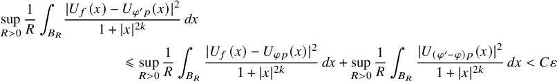 $$ \begin{align*} \sup_{R>0}\frac1R\int_{B_R} &\frac{|U_f(x)-U_{\varphi' p}(x)|^2}{1+|x|^{2k}}\, dx\\ &\qquad\qquad \leqslant \sup_{R>0}\frac1R\int_{B_R} \frac{|U_{f}(x)-U_{\varphi p}(x)|^2}{1+|x|^{2k}}\, dx+ \sup_{R>0}\frac1R\int_{B_R} \frac{|U_{(\varphi'-\varphi)p}(x)|^2}{1+|x|^{2k}}\, dx <C\varepsilon \end{align*} $$
provided that $\|\varphi -\varphi '\|_{H^{-k}({\mathbb {S}})}<\varepsilon -\varepsilon '$
.
$\|\varphi -\varphi '\|_{H^{-k}({\mathbb {S}})}<\varepsilon -\varepsilon '$
.
Finally, to see that $\varepsilon _{f,0}=0$
if
$\varepsilon _{f,0}=0$
if $f\in L^2({\mathbb {S}},{\mathbb {C}}^3)$
, let us take a smooth function
$f\in L^2({\mathbb {S}},{\mathbb {C}}^3)$
, let us take a smooth function $\Theta :{\mathbb {R}}^3\to [0,1]$
supported in the unit ball and such that
$\Theta :{\mathbb {R}}^3\to [0,1]$
supported in the unit ball and such that $\Theta (0)=1$
. Setting
$\Theta (0)=1$
. Setting
 $$\begin{align*}\Theta_n(\xi):= \Theta(n \xi- n\xi_+) + \Theta(n \xi- n\xi_-)\,, \end{align*}$$
we trivially get that $\|\Theta _n f\|_{L^2({\mathbb {S}})}\leqslant \|f\|_{L^2({\mathbb {S}})}$
for all
$\|\Theta _n f\|_{L^2({\mathbb {S}})}\leqslant \|f\|_{L^2({\mathbb {S}})}$
for all $n\geqslant 2$
and that
$n\geqslant 2$
and that $\Theta _n f$
tends to zero almost everywhere in
$\Theta _n f$
tends to zero almost everywhere in ${\mathbb {S}}$
as
${\mathbb {S}}$
as $n\to \infty $
. The dominated convergence theorem then shows that
$n\to \infty $
. The dominated convergence theorem then shows that $\|\Theta _n f\|_{L^2({\mathbb {S}})}\to 0$
as
$\|\Theta _n f\|_{L^2({\mathbb {S}})}\to 0$
as $n\to \infty $
, thus proving the claim.
$n\to \infty $
, thus proving the claim.
Another, rather different in spirit, formulation of the principle that densities of the form $\varphi p$
can approximate general Beltrami fields is presented in the following theorem. Unlike the previous corollary, the approximation is considered only locally in space, and in this direction, one shows that even considering smooth functions
$\varphi p$
can approximate general Beltrami fields is presented in the following theorem. Unlike the previous corollary, the approximation is considered only locally in space, and in this direction, one shows that even considering smooth functions $\varphi $
is enough to obtain a subset of Beltrami fields that is dense in the
$\varphi $
is enough to obtain a subset of Beltrami fields that is dense in the $C^k$
compact-open topology:
$C^k$
compact-open topology:
Proposition 2.5. Fix any positive reals $\varepsilon $
and k and a compact set
$\varepsilon $
and k and a compact set $K\subset {\mathbb {R}}^3$
such that
$K\subset {\mathbb {R}}^3$
such that ${\mathbb {R}}^3\backslash K$
is connected. Then, given any vector field v satisfying the equation
${\mathbb {R}}^3\backslash K$
is connected. Then, given any vector field v satisfying the equation $\operatorname {\mathrm {curl}} v=v$
in an open neighborhood of K, there exists a Hermitian finite linear combination of spherical harmonics
$\operatorname {\mathrm {curl}} v=v$
in an open neighborhood of K, there exists a Hermitian finite linear combination of spherical harmonics $\varphi $
such that the Beltrami field
$\varphi $
such that the Beltrami field $U_{\varphi p}$
approximates v in the set K as
$U_{\varphi p}$
approximates v in the set K as
 $$\begin{align*}\|U_{\varphi p}-v\|_{C^k(K)}<\varepsilon\,. \end{align*}$$
Proof. Let us fix an open set $V\supset K$
whose closure is contained in the open neighborhood where v is defined, and a large ball
$V\supset K$
whose closure is contained in the open neighborhood where v is defined, and a large ball $B_R\supset \overline V$
. Since
$B_R\supset \overline V$
. Since $\mathbb R^3\backslash K$
is connected, it is obvious that we can take V so that
$\mathbb R^3\backslash K$
is connected, it is obvious that we can take V so that $\mathbb R^3\backslash \overline V$
is connected as well. By the approximation theorem with decay for Beltrami fields [Reference Enciso and Peralta-Salas14, Theorem 8.3], there is a Beltrami field w that approximates v as
$\mathbb R^3\backslash \overline V$
is connected as well. By the approximation theorem with decay for Beltrami fields [Reference Enciso and Peralta-Salas14, Theorem 8.3], there is a Beltrami field w that approximates v as
 $$\begin{align*}\|w-v\|_{C^k(V)}<\varepsilon \end{align*}$$
and is bounded as $|w(x)|<C/|x|$
. As the Fourier transform of w is supported on
$|w(x)|<C/|x|$
. As the Fourier transform of w is supported on ${\mathbb {S}}$
, Herglotz’s theorem [Reference Hörmander26, Theorem 7.1.28] shows that one can write
${\mathbb {S}}$
, Herglotz’s theorem [Reference Hörmander26, Theorem 7.1.28] shows that one can write $w=U_f$
for some vector-valued Hermitian field
$w=U_f$
for some vector-valued Hermitian field $f\in L^2({\mathbb {S}},{\mathbb {C}}^3)$
that satisfies the distributional equation (2.2). Proposition 2.4 then shows that there exists some Hermitian scalar function
$f\in L^2({\mathbb {S}},{\mathbb {C}}^3)$
that satisfies the distributional equation (2.2). Proposition 2.4 then shows that there exists some Hermitian scalar function $\varphi \in C^{\infty }({\mathbb {S}})$
such that
$\varphi \in C^{\infty }({\mathbb {S}})$
such that
 $$\begin{align*}\|U_f-U_{\varphi p}\|_{L^2(B_R)}<C\varepsilon\, \end{align*}$$
so that
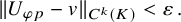
 $\|v-U_{\varphi p}\|_{L^2(V)}<C\varepsilon $
. As the difference
$\|v-U_{\varphi p}\|_{L^2(V)}<C\varepsilon $
. As the difference $v-U_{\varphi p}$
satisfies the Helmholtz equation
$v-U_{\varphi p}$
satisfies the Helmholtz equation
 $$\begin{align*}{\Delta} (v-U_{\varphi p}) + v-U_{\varphi p}=0 \end{align*}$$
in V, and $K\subset \!\subset V$
, standard elliptic estimates then allow us to promote this bound to
$K\subset \!\subset V$
, standard elliptic estimates then allow us to promote this bound to
 $$\begin{align*}\|v-U_{\varphi p}\|_{C^k(K)}<C\varepsilon\,, \end{align*}$$
as we wished to prove.
3 Gaussian random Beltrami fields
The Fourier-theoretical characterization of Beltrami fields presented in the previous section paves the way to the definition of random Beltrami fields.
In parallel with equation (1.3a) (see Appendix A for further heuristics), let us start by setting
 $$\begin{align*}\varphi(\xi) := \sum_{l=0}^{\infty}\sum_{m=-l}^{l} i^l \, a_{ l m}\,Y_{lm}(\xi)\,, \end{align*}$$
where $a_{l m}$
are normally distributed independent standard Gaussian random variables and
$a_{l m}$
are normally distributed independent standard Gaussian random variables and $Y_{lm}$
is an orthonormal basis of (real-valued) spherical harmonics on
$Y_{lm}$
is an orthonormal basis of (real-valued) spherical harmonics on ${\mathbb {S}}$
. Note that
${\mathbb {S}}$
. Note that $\varphi $
is Hermitian because of the identity
$\varphi $
is Hermitian because of the identity $Y_{lm}(-\xi )=(-1)^ l Y_{lm}(\xi )$
. We now define a Gaussian random Beltrami field as
$Y_{lm}(-\xi )=(-1)^ l Y_{lm}(\xi )$
. We now define a Gaussian random Beltrami field as
 $$\begin{align*}u:= U_{\varphi p}\,, \end{align*}$$
where we recall that $U_f$
and p were respectively defined in equations (2.1) and (2.4).
$U_f$
and p were respectively defined in equations (2.1) and (2.4).
Remark 3.1. As discussed in Proposition 2.1, the role of the vector field p is to ensure that the density $f:=\varphi p$
satisfies the Beltrami equation in Fourier space,
$f:=\varphi p$
satisfies the Beltrami equation in Fourier space, $i\xi \times f(\xi )=f(\xi )$
. Hence, one could replace
$i\xi \times f(\xi )=f(\xi )$
. Hence, one could replace $p(\xi )$
by any nonvanishing multiple of it, that is, by
$p(\xi )$
by any nonvanishing multiple of it, that is, by $\widetilde p(\xi ):= \Lambda (\xi )\, p(\xi )$
, where
$\widetilde p(\xi ):= \Lambda (\xi )\, p(\xi )$
, where $\Lambda :{\mathbb {R}}^3\to {\mathbb {C}}$
is a smooth scalar Hermitian function that does not vanish on
$\Lambda :{\mathbb {R}}^3\to {\mathbb {C}}$
is a smooth scalar Hermitian function that does not vanish on ${\mathbb {S}}$
. All the results of the paper about random Beltrami fields remain valid if one defines a Gaussian random Beltrami field as
${\mathbb {S}}$
. All the results of the paper about random Beltrami fields remain valid if one defines a Gaussian random Beltrami field as $u:= U_{\varphi \widetilde p}$
with
$u:= U_{\varphi \widetilde p}$
with $\varphi $
as above, provided that one replaces p by
$\varphi $
as above, provided that one replaces p by $\widetilde p$
in the formulas. Also, the results do not change if one replaces the basis of spherical harmonics by any other orthonormal basis of
$\widetilde p$
in the formulas. Also, the results do not change if one replaces the basis of spherical harmonics by any other orthonormal basis of $L^2({\mathbb {S}})$
, but this choice leads to slightly more explicit formulas for certain intermediate objects that appear in the proofs.
$L^2({\mathbb {S}})$
, but this choice leads to slightly more explicit formulas for certain intermediate objects that appear in the proofs.
In what follows, we will use the notation $D:= -i\nabla $
. An important role will be played by the vector-valued differential operator with real coefficients
$D:= -i\nabla $
. An important role will be played by the vector-valued differential operator with real coefficients $p(D)$
, whose expression in Fourier space is
$p(D)$
, whose expression in Fourier space is
 $$\begin{align*}\widehat{p(D)\psi}(\xi)=p(\xi)\, \widehat\psi(\xi)\,, \end{align*}$$
for any scalar function $\psi $
in
$\psi $
in $\mathbb R^3$
. Equivalently, by Remark 2.2, the operator
$\mathbb R^3$
. Equivalently, by Remark 2.2, the operator $p(D)$
reads, in physical space, as
$p(D)$
reads, in physical space, as
 $$\begin{align*}p(D)\psi=-(\operatorname{\mathrm{curl}} \operatorname{\mathrm{curl}}+\operatorname{\mathrm{curl}})(q(D_1)\psi,0,0)\,, \end{align*}$$
where $D_1:= -i{\partial }_{x_1}$
.
$D_1:= -i{\partial }_{x_1}$
.
The first result of this section shows that a Gaussian random Beltrami field is a well-defined object both in Fourier and physical spaces.
Proposition 3.2. With probability $1$
, the function
$1$
, the function $\varphi $
is in
$\varphi $
is in $H^{-1-\delta }({\mathbb {S}})\backslash L^2({\mathbb {S}})$
for any
$H^{-1-\delta }({\mathbb {S}})\backslash L^2({\mathbb {S}})$
for any $\delta>0$
. In particular, almost surely, u is a
$\delta>0$
. In particular, almost surely, u is a $C^{\infty }$
vector field and can be written as
$C^{\infty }$
vector field and can be written as
 $$ \begin{align} u(x)=(2\pi)^{\frac{3}{2}}\sum_{l=0}^{\infty}\sum_{m=-l}^{l} \, a_{ l m}\, p(D)\left[Y_{lm} \left(\frac{x}{|x|}\right) \frac{J_{ l + \frac12}(|x|)}{|x|^{1/2}}\right]\,. \end{align} $$
The series converges in $C^k$
uniformly on compact sets almost surely, for any k.
$C^k$
uniformly on compact sets almost surely, for any k.
Proof. For $l\geqslant 0$
and
$l\geqslant 0$
and $-l\leqslant m\leqslant l$
,
$-l\leqslant m\leqslant l$
, $a_{lm}^2$
are independent, identically distributed random variables with expected value 1. As the number of these variables with
$a_{lm}^2$
are independent, identically distributed random variables with expected value 1. As the number of these variables with $l\leqslant n$
is
$l\leqslant n$
is
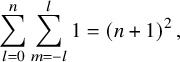 $$\begin{align*}\sum_{l=0}^n\sum_{m=-l}^{l}1=(n+1)^2\,, \end{align*}$$
the strong law of large numbers ensures that the sample average, that is, the random variable
 $$\begin{align*}X_n:=\frac1{(n+1)^2}\sum_{l=0}^n\sum_{m=-l}^{l}a_{ l m}^2\,, \end{align*}$$
converges to 1 almost surely as $n\to \infty $
. Now, consider the truncation
$n\to \infty $
. Now, consider the truncation
 $$\begin{align*}\varphi_n(\xi) := \sum_{l=0}^n\sum_{m=-l}^{l} i^l \, a_{ l m}\,Y_{lm}(\xi)\,. \end{align*}$$
As the spherical harmonics $Y_{lm}$
are orthonormal, the
$Y_{lm}$
are orthonormal, the $L^2$
norm of
$L^2$
norm of $\varphi _n$
is
$\varphi _n$
is
 $$\begin{align*}\|\varphi_n\|_{L^2({\mathbb{S}})}^2=\sum_{l=0}^n\sum_{m=-l}^{l}a_{ l m}^2= (n+1)^2 X_n\,, \end{align*}$$
and $\|\varphi _n\|_{L^2({\mathbb {S}})}^2$
tends to
$\|\varphi _n\|_{L^2({\mathbb {S}})}^2$
tends to $\|\varphi \|_{L^2({\mathbb {S}})}^2$
(which may be infinite) as
$\|\varphi \|_{L^2({\mathbb {S}})}^2$
(which may be infinite) as $n\to \infty $
. Since
$n\to \infty $
. Since $X_n\to 1$
almost surely, we obtain from the above formula that
$X_n\to 1$
almost surely, we obtain from the above formula that $(n+1)^{-2}\|\varphi _n\|_{L^2({\mathbb {S}})}^2$
tends to 1 almost surely. Therefore,
$(n+1)^{-2}\|\varphi _n\|_{L^2({\mathbb {S}})}^2$
tends to 1 almost surely. Therefore, $\varphi $
is not in
$\varphi $
is not in $L^2({\mathbb {S}})$
with probability 1.
$L^2({\mathbb {S}})$
with probability 1.
On the other hand, since
 $$\begin{align*}\|\varphi\|_{H^{-s}({\mathbb{S}})}^2=\sum_{l=0}^{\infty}\sum_{m=-l}^{l}\frac{a_{ l m}^2}{(l+1)^{2s}}\,, \end{align*}$$
it is straightforward to see that the expected value
 $$\begin{align*}{\mathbb{E}}\|\varphi\|_{H^{-1-\delta}({\mathbb{S}})}^2=\sum_{l=0}^{\infty}\sum_{m=-l}^{l}\frac{{\mathbb{E}} a_{ l m}^2}{(l+1)^{2+2\delta}}= \sum_{l=0}^{\infty}\frac{2l+1}{(l+1)^{2+2\delta}} \end{align*}$$
is finite for all $\delta>0$
. Hence,
$\delta>0$
. Hence, $\varphi \in H^{-1-\delta }({\mathbb {S}})$
almost surely, so
$\varphi \in H^{-1-\delta }({\mathbb {S}})$
almost surely, so $u:= U_{\varphi p}$
is well-defined with probability 1.
$u:= U_{\varphi p}$
is well-defined with probability 1.
To prove the representation formula for u and its convergence, let us begin by noting that
 $$ \begin{align*} U_{i^l Y_{lm} p}(x)&= \int_{\mathbb{S}} i^l p(\xi) \,Y_{lm}(\xi)\, e^{i\xi\cdot x}\, d{\sigma}(\xi)\\ &= p(D)\int_{\mathbb{S}} i^l Y_{lm}(\xi)\, e^{i\xi\cdot x}\, d{\sigma}(\xi)\,. \end{align*} $$
Using either the theory of point pair invariants and zonal spherical functions [Reference Canzani and Sarnak8, Proposition 4] or special function identities [Reference Enciso, Peralta-Salas and Romaniega15, Proposition 2.1], the Fourier transform of $Y_{lm}\, d{\sigma }$
has been shown to be
$Y_{lm}\, d{\sigma }$
has been shown to be
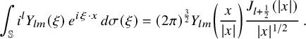 $$\begin{align*}\int_{\mathbb{S}} i^l Y_{lm}(\xi)\, e^{i\xi\cdot x}\, d{\sigma}(\xi)= (2\pi)^{\frac32} Y_{lm} \left(\frac{x}{|x|}\right) \frac{J_{ l + \frac12}(|x|)}{|x|^{1/2}}\,. \end{align*}$$
This permits to formally write u as equation (3.1). To show that this series converges in $C^k$
on compact sets, for any large n, any
$C^k$
on compact sets, for any large n, any $N>n$
and any fixed positive integer k consider the quantity
$N>n$
and any fixed positive integer k consider the quantity
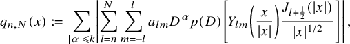 $$\begin{align*}q_{n,N}(x):= \sum_{|{\alpha}|\leqslant k} \left|\sum_{l=n}^N \sum_{m=-l}^l a_{lm} D^{\alpha} p(D)\left[Y_{lm} \left(\frac{x}{|x|}\right) \frac{J_{ l + \frac12}(|x|)}{|x|^{1/2}}\right]\right|\,, \end{align*}$$
where we are using the standard multi-index notation. Since $p(D)$
is a third-order operator, for all
$p(D)$
is a third-order operator, for all $|x|<R$
we obviously have
$|x|<R$
we obviously have
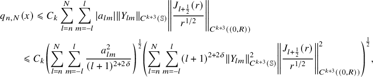 $$ \begin{align*} q_{n,N}&(x)\leqslant C_k \sum_{l=n}^N \sum_{m=-l}^l |a_{lm}|\|Y_{lm}\|_{C^{k+3}({\mathbb{S}})}\left\| \frac{J_{ l + \frac12}(r)}{r^{1/2}}\right\|_{C^{k+3}((0,R))}\\ &\leqslant C_k \left(\sum_{l=n}^N \sum_{m=-l}^l \frac{a_{lm}^2}{(l+1)^{2+2\delta}}\right)^{\frac12}\left(\sum_{l=n}^N \sum_{m=-l}^l(l+1)^{2+2\delta} \|Y_{lm}\|_{C^{k+3}({\mathbb{S}})}^2 \left\| \frac{J_{ l + \frac12}(r)}{r^{1/2}}\right\|^2_{C^{k+3}((0,R))}\right)^{\frac12}, \end{align*} $$
where here $r:=|x|$
and we have used the Cauchy–Schwartz inequality to pass to the second line. The Sobolev inequality immediately gives
$r:=|x|$
and we have used the Cauchy–Schwartz inequality to pass to the second line. The Sobolev inequality immediately gives
 $$\begin{align*}\|Y_{lm}\|_{C^{k+3}({\mathbb{S}})}\leqslant C\|Y_{lm}\|_{H^{k+5}({\mathbb{S}})}\leqslant C(l+1)^{k+5}\,. \end{align*}$$
To estimate the Bessel function, recall the large-degree asymptotics
 $$\begin{align*}J_{\nu}(r)\sim (2\pi\nu)^{-\frac12} \left(\frac{er}{2\nu}\right)^{\nu}\,, \end{align*}$$
which holds as $\nu \to \infty $
for uniformly bounded r. As the derivative of a Bessel function can be written in terms of Bessel functions via the recurrence relation
$\nu \to \infty $
for uniformly bounded r. As the derivative of a Bessel function can be written in terms of Bessel functions via the recurrence relation
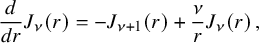 $$\begin{align*}\frac d{dr}J_{\nu}(r)= -J_{\nu+1}(r) + \frac\nu r J_{\nu}(r)\,, \end{align*}$$
it follows that the $C^{k+3}$
norm of
$C^{k+3}$
norm of $J_{l+\frac 12}(r)/r^{1/2}$
tends to 0 exponentially as
$J_{l+\frac 12}(r)/r^{1/2}$
tends to 0 exponentially as $l\to \infty $
on compact sets:
$l\to \infty $
on compact sets:
 $$\begin{align*}\left\| \frac{J_{ l + \frac12}(r)}{r^{1/2}}\right\|_{C^{k+3}((0,R))}\leqslant \left(\frac{CR}{l}\right)^{l-k-3}\,. \end{align*}$$
Since we have proven that
 $$\begin{align*}\sum_{l=0}^{\infty}\sum_{m=-l}^l \frac{a_{lm}^2}{(l+1)^{2+2\delta}}<\infty \end{align*}$$
almost surely, now one only has to put together the estimates above to see that, almost surely, $q_{n,N}(x)$
tends to 0 as
$q_{n,N}(x)$
tends to 0 as $n\to \infty $
uniformly for all
$n\to \infty $
uniformly for all $N>n$
and for all x in a compact subset of
$N>n$
and for all x in a compact subset of ${\mathbb {R}}^3$
. This establishes the convergence of the series and completes the proof of the proposition.
${\mathbb {R}}^3$
. This establishes the convergence of the series and completes the proof of the proposition.
Remark 3.3. Note that each summand $U_{i^l Y_{lm}p}=(2\pi )^{3/2}p(D)[Y_{lm} (\frac {x}{|x|}) |x|^{-1/2} {J_{ l + \frac 12}(|x|)}]$
of the series (3.1) is a Beltrami field.
$U_{i^l Y_{lm}p}=(2\pi )^{3/2}p(D)[Y_{lm} (\frac {x}{|x|}) |x|^{-1/2} {J_{ l + \frac 12}(|x|)}]$
of the series (3.1) is a Beltrami field.
Since $a_{lm}$
are standard Gaussian variables, it is obvious that the vector-valued Gaussian field u has zero mean. Our next goal is to compute its covariance kernel,
$a_{lm}$
are standard Gaussian variables, it is obvious that the vector-valued Gaussian field u has zero mean. Our next goal is to compute its covariance kernel, $\kappa $
, which maps each pair of points
$\kappa $
, which maps each pair of points $(x,y)\in {\mathbb {R}}^3\times {\mathbb {R}}^3$
to the symmetric
$(x,y)\in {\mathbb {R}}^3\times {\mathbb {R}}^3$
to the symmetric $3\times 3$
matrix
$3\times 3$
matrix
 $$ \begin{align} \kappa(x,y):={\mathbb{E}}[u(x)\otimes u(y)]\,. \end{align} $$
In particular, we show that this kernel is translationally invariant, meaning that it only depends on the difference:
 $$\begin{align*}\kappa(x,y)=\varkappa(x-y)\,. \end{align*}$$
We recall that, by Bochner’s theorem, there exists a nonnegative-definite matrix-valued measure $\rho $
such that
$\rho $
such that $\varkappa $
is the Fourier transform of
$\varkappa $
is the Fourier transform of $\rho $
: This is the spectral measure of the Gaussian random field u. In the statement,
$\rho $
: This is the spectral measure of the Gaussian random field u. In the statement, $p_j$
is the
$p_j$
is the $j^{\text {th}}$
component of the vector field p.
$j^{\text {th}}$
component of the vector field p.
Proposition 3.4. The components of the covariance kernel of the Gaussian random field u are
 $$\begin{align*}\kappa_{jk}(x,y)= \varkappa_{jk}(x-y) \end{align*}$$
with
 $$\begin{align*}\varkappa_{jk}(x):= (2\pi)^{\frac32} p_j(D) p_k(-D)\frac{J_{1/2}(|x|)}{|x|^{1/2}}\,. \end{align*}$$
The spectral measure is $d\rho (\xi )= p(\xi )\otimes \overline {p(\xi )}\, d{\sigma }(\xi )$
.
$d\rho (\xi )= p(\xi )\otimes \overline {p(\xi )}\, d{\sigma }(\xi )$
.
Proof. As $a_{lm}$
are independent standard Gaussian variables,
$a_{lm}$
are independent standard Gaussian variables, ${\mathbb {E}}(a_{lm}a_{l'm'})=\delta _{ll'}\delta _{mm'}$
, so the covariance matrix is
${\mathbb {E}}(a_{lm}a_{l'm'})=\delta _{ll'}\delta _{mm'}$
, so the covariance matrix is
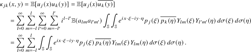 $$ \begin{align*} \kappa_{jk}&(x,y)= {\mathbb{E}}[u_j(x) u_k(y)]={\mathbb{E}}[u_j(x) \overline{u_k(y)}]\\ &= \sum_{l=0}^{\infty}\sum_{m=-l}^l \sum_{l'=0}^{\infty}\sum_{m=-l'}^{l'} i^{l-l'}{\mathbb{E}}(a_{lm}a_{l'm'})\int_{\mathbb{S}}\int_{\mathbb{S}} e^{ix\cdot \xi-iy\cdot \eta} p_j(\xi)\, \overline{p_k(\eta)}\, Y_{lm}(\xi)\,{Y_{l'm'}(\eta)}\, d{\sigma}(\xi)\, d{\sigma}(\eta)\\ &= \sum_{l=0}^{\infty}\sum_{m=-l}^l \int_{\mathbb{S}}\int_{\mathbb{S}} e^{ix\cdot \xi-iy\cdot \eta} p_j(\xi)\, \overline{p_k(\eta)}\, Y_{lm}(\xi)\,{Y_{lm}(\eta)}\, d{\sigma}(\xi)\, d{\sigma}(\eta)\,. \end{align*} $$
Here, we have used that u and the spherical harmonics $Y_{lm}$
are real-valued. Since
$Y_{lm}$
are real-valued. Since $Y_{lm}$
is an orthonormal basis, one has that
$Y_{lm}$
is an orthonormal basis, one has that
 $$\begin{align*}\sum_{l=0}^{\infty}\sum_{m=-l}^l \int_{\mathbb{S}}\int_{\mathbb{S}} \psi(\xi)\,\phi(\eta)\, Y_{lm}(\xi)\, Y_{lm}(\eta)\, d{\sigma}(\xi)\, d{\sigma}(\eta)=\int_{\mathbb{S}} \psi(\xi)\,\phi(\xi)\, d{\sigma}(\xi) \end{align*}$$
for any functions $\psi ,\phi \in L^2({\mathbb {S}})$
. Hence, we can get rid of the sums in the above formula and write
$\psi ,\phi \in L^2({\mathbb {S}})$
. Hence, we can get rid of the sums in the above formula and write
 $$ \begin{align} \kappa_{jk}(x,y)& = \int_{\mathbb{S}} e^{i(x-y)\cdot\xi}\,p_j(\xi)\, \overline{p_k(\xi)} \, d{\sigma}(\xi)\,, \end{align} $$
which yields the formula for the spectral measure of u. Using now that p is Hermitian (i.e., $\overline { p(\xi )}=p(-\xi )$
) and a well-known representation formula for the Bessel function
$\overline { p(\xi )}=p(-\xi )$
) and a well-known representation formula for the Bessel function $J_{1/2}$
, the above integral can be equivalently written as
$J_{1/2}$
, the above integral can be equivalently written as
 $$ \begin{align*} \int_{\mathbb{S}} e^{ix\cdot\xi}\, p_j(\xi)\, \overline{p_k(\xi)}\, d{\sigma}(\xi)&= p_j(D)\, {p_k(-D)}\int_{\mathbb{S}} e^{ix\cdot\xi} d{\sigma}(\xi)\\ &= (2\pi)^{\frac32}p_j(D)\, {p_k(-D)}\frac{J_{1/2}(|x|)}{|x|^{1/2}}\,. \end{align*} $$
The proposition then follows.
Remark 3.5. A random vector field is called isotropic if its covariance kernel is invariant under rotations, that is, for any Euclidean rotation R we have
 $$ \begin{align*}\mathbb{E}\left(R_*u(x)\otimes R_*u(y)\right)=\mathbb{E}\left(u(x)\otimes u(y)\right)\,, \end{align*} $$
where $R_*$
denotes the push-forward of u under the action of R. It is well known that the most general form of a symmetric
$R_*$
denotes the push-forward of u under the action of R. It is well known that the most general form of a symmetric $3\times 3$
matrix function in
$3\times 3$
matrix function in ${\mathbb {R}}^3$
that is invariant under spherical rotations is
${\mathbb {R}}^3$
that is invariant under spherical rotations is
 $$\begin{align*}f_1(|x|)I+f_2(|x|)x\otimes x\,, \end{align*}$$
where $f_1$
and
$f_1$
and $f_2$
are arbitrary functions of
$f_2$
are arbitrary functions of $|x|$
. From equation (3.3), we see that our random Beltrami field is not isotropic because
$|x|$
. From equation (3.3), we see that our random Beltrami field is not isotropic because $p(\xi )\otimes \overline {p(\xi )}$
is not of the form
$p(\xi )\otimes \overline {p(\xi )}$
is not of the form $a I+b\xi \otimes \xi $
for some constants
$a I+b\xi \otimes \xi $
for some constants $a,b$
on
$a,b$
on ${\mathbb {S}}$
. This property is not an issue of our construction and cannot be fixed by changing the vector field
${\mathbb {S}}$
. This property is not an issue of our construction and cannot be fixed by changing the vector field $p(\xi )$
. This is in strong contrast with the random vector field
$p(\xi )$
. This is in strong contrast with the random vector field
![]() , where F is the Gaussian random monochromatic wave defined in (1.3b). It is not difficult to show that
, where F is the Gaussian random monochromatic wave defined in (1.3b). It is not difficult to show that
 $$\begin{align*}\mathbb{E}\left(\hat{u}_j(x)\hat{u}_k(y)\right)= \int_{\mathbb{S}} e^{i(x-y)\cdot\xi}\,\hat{p}_j(\xi)\, \overline{\hat{p}_k(\xi)} \, d{\sigma}(\xi)\,, \end{align*}$$
where now $\hat {p}_j(\xi ):=i\xi _j$
, and hence
$\hat {p}_j(\xi ):=i\xi _j$
, and hence $\hat u$
is an isotropic field. However, it is worth noting that, in both cases, the random vector field is constructed from an isotropic scalar field, and the spectral measure of the vector field is the spectral measure of the isotropic scalar field times a tensor product of polynomials. In the case of the gradient, the matrix covariance kernel is the Hessian of the scalar covariance kernel, so it is isotropic. In contrast, in the case of the Beltrami field, the derivatives are more involved because of the differential equation the field must satisfy.
$\hat u$
is an isotropic field. However, it is worth noting that, in both cases, the random vector field is constructed from an isotropic scalar field, and the spectral measure of the vector field is the spectral measure of the isotropic scalar field times a tensor product of polynomials. In the case of the gradient, the matrix covariance kernel is the Hessian of the scalar covariance kernel, so it is isotropic. In contrast, in the case of the Beltrami field, the derivatives are more involved because of the differential equation the field must satisfy.
A straightforward corollary is that the Gaussian random Beltrami field u is normalized so that its covariance matrix is the identity on the diagonal.
Corollary 3.6. For any $x\in {\mathbb {R}}^3$
,
$x\in {\mathbb {R}}^3$
, $\kappa (x,x)=I$
.
$\kappa (x,x)=I$
.
Proof. The formula for the spectral measure computed in Proposition 3.4 implies that
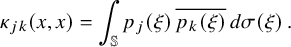 $$\begin{align*}\kappa_{jk}(x,x)=\int_{\mathbb{S}} p_j(\xi)\, \overline{p_k(\xi)}\, d{\sigma}(\xi)\,. \end{align*}$$
As p is a polynomial, the computation then boils down to evaluating integrals of the form $\int _{\mathbb {S}} \xi ^{\alpha }\, d{\sigma }(\xi )$
, where
$\int _{\mathbb {S}} \xi ^{\alpha }\, d{\sigma }(\xi )$
, where ${\alpha }=({\alpha }_1,{\alpha }_2,{\alpha }_3)$
is a multi-index and
${\alpha }=({\alpha }_1,{\alpha }_2,{\alpha }_3)$
is a multi-index and $\xi ^{\alpha }:=\xi _1^{{\alpha }_1}\xi _2^{{\alpha }_2}\xi _3^{{\alpha }_3}$
. These integrals can be computed in closed form [Reference Folland18]:
$\xi ^{\alpha }:=\xi _1^{{\alpha }_1}\xi _2^{{\alpha }_2}\xi _3^{{\alpha }_3}$
. These integrals can be computed in closed form [Reference Folland18]:
 $$ \begin{align} \int_{\mathbb{S}} \xi^{\alpha}\, d{\sigma}(\xi)= \begin{cases} 2\big[\prod_{j=1}^3\Gamma(\frac{{\alpha}_j+1}2)\big] /\Gamma(\frac{|{\alpha}|+3}2) & \text{if } {\alpha}_1,{\alpha}_2,{\alpha}_3 \text{ are even,}\\[1mm] 0 & \text{otherwise.} \end{cases} \end{align} $$
Here, $\Gamma $
denotes the gamma function.
$\Gamma $
denotes the gamma function.
Armed with this formula and taking into account the explicit expression of the polynomial $p(\xi )$
(cf. equation (2.4)), a tedious but straightforward computation shows
$p(\xi )$
(cf. equation (2.4)), a tedious but straightforward computation shows
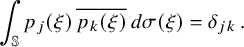 $$\begin{align*}\int_{\mathbb{S}} p_j(\xi)\, \overline{p_k(\xi)}\, d{\sigma}(\xi)=\delta_{jk}\,. \end{align*}$$
The result then follows.
Remark 3.7. The probability density function of the Gaussian random vector $u(x)$
is therefore
$u(x)$
is therefore $\rho (y):= (2\pi )^{-\frac 32}\, e^{-\frac 12|y|^2}$
. That is,
$\rho (y):= (2\pi )^{-\frac 32}\, e^{-\frac 12|y|^2}$
. That is, ${\mathbb {P}}\{u(x)\in \Omega \}= \int _{\Omega }\rho (y)\, dy $
for any
${\mathbb {P}}\{u(x)\in \Omega \}= \int _{\Omega }\rho (y)\, dy $
for any $x\in {\mathbb {R}}^3$
and any Borel subset
$x\in {\mathbb {R}}^3$
and any Borel subset $\Omega \subset {\mathbb {R}}^3$
.
$\Omega \subset {\mathbb {R}}^3$
.
Since the Gaussian field u is of class $C^{\infty }$
with probability 1 by Proposition 3.2, it is standard that it defines a Gaussian probability measure, which we henceforth denote by
$C^{\infty }$
with probability 1 by Proposition 3.2, it is standard that it defines a Gaussian probability measure, which we henceforth denote by ${\mu _u}$
, on the space of
${\mu _u}$
, on the space of $C^k$
vector fields on
$C^k$
vector fields on ${\mathbb {R}}^3$
, where k is any fixed positive integer. This space is endowed with its usual Borel
${\mathbb {R}}^3$
, where k is any fixed positive integer. This space is endowed with its usual Borel ${\sigma }$
-algebra
${\sigma }$
-algebra ${\mathfrak {S}}$
, which is the minimal
${\mathfrak {S}}$
, which is the minimal ${\sigma }$
-algebra containing the ‘squares’
${\sigma }$
-algebra containing the ‘squares’
 $$\begin{align*}I(x,a,b):= \{w\in C^k({\mathbb{R}}^3,{\mathbb{R}}^3): w(x)\in[a_1,b_1)\times [a_2,b_2)\times[a_3,b_3)\} \end{align*}$$
for all $x,a,b,\in {\mathbb {R}}^3$
. To spell out the details, let us denote by
$x,a,b,\in {\mathbb {R}}^3$
. To spell out the details, let us denote by $\Omega $
the sample space of the random variables
$\Omega $
the sample space of the random variables $a_{lm}$
and show that the random field u is a measurable map from
$a_{lm}$
and show that the random field u is a measurable map from $\Omega $
to
$\Omega $
to $C^k({\mathbb {R}}^3,{\mathbb {R}}^3)$
. Since the
$C^k({\mathbb {R}}^3,{\mathbb {R}}^3)$
. Since the ${\sigma }$
-algebra of
${\sigma }$
-algebra of $C^k({\mathbb {R}}^3,{\mathbb {R}}^3)$
is generated by point evaluations, it suffices to show that
$C^k({\mathbb {R}}^3,{\mathbb {R}}^3)$
is generated by point evaluations, it suffices to show that
 $$\begin{align*}u(x)= \sum_{l=0}^{\infty} \sum_{m=-l}^l a_{lm}\, U_{i^l Y_{lm}p}(x) \end{align*}$$
is a measurable function $\Omega \to {\mathbb {R}}^3$
for each
$\Omega \to {\mathbb {R}}^3$
for each $x\in {\mathbb {R}}^3$
. But this is obvious because
$x\in {\mathbb {R}}^3$
. But this is obvious because $u(x)$
is the limit of finite linear combinations (with coefficients in
$u(x)$
is the limit of finite linear combinations (with coefficients in ${\mathbb {R}}^3$
) of the random variables
${\mathbb {R}}^3$
) of the random variables $a_{lm}$
, which are of course measurable. In what follows, we will not mention the
$a_{lm}$
, which are of course measurable. In what follows, we will not mention the ${\sigma }$
-algebra explicitly to keep the notation simple. Also, in view of the later applications to invariant tori, we will henceforth assume that
${\sigma }$
-algebra explicitly to keep the notation simple. Also, in view of the later applications to invariant tori, we will henceforth assume that $k\geqslant 4$
. Obviously, the Gaussian probability measure
$k\geqslant 4$
. Obviously, the Gaussian probability measure ${\mu _u}$
is regular because the space of
${\mu _u}$
is regular because the space of $C^k$
vector fields is metrizable (with the compact-open
$C^k$
vector fields is metrizable (with the compact-open $C^k$
-topology).
$C^k$
-topology).
Following Nazarov and Sodin [Reference Nazarov and Sodin30], the next proposition shows two useful properties of our Gaussian probability measure that will be extensively employed in the rest of the paper. They easily follow from the facts that the covariance kernel $\kappa (x,y)$
only depends on
$\kappa (x,y)$
only depends on $x-y$
and that the spectral measure has no atoms. Before stating the result, let us recall that the probability measure
$x-y$
and that the spectral measure has no atoms. Before stating the result, let us recall that the probability measure ${\mu _u}$
is said to be translationally invariant if
${\mu _u}$
is said to be translationally invariant if ${\mu _u}(\tau _y {\mathcal {A}})={\mu _u}({\mathcal {A}})$
for all
${\mu _u}(\tau _y {\mathcal {A}})={\mu _u}({\mathcal {A}})$
for all ${\mathcal {A}}\subset {\mathfrak {S}}$
and all
${\mathcal {A}}\subset {\mathfrak {S}}$
and all $y\in {\mathbb {R}}^3$
. Here,
$y\in {\mathbb {R}}^3$
. Here, $\tau _y$
denotes the translation operator on
$\tau _y$
denotes the translation operator on $C^k$
fields, defined as
$C^k$
fields, defined as $\tau _y w(x):= w(x+y)$
.
$\tau _y w(x):= w(x+y)$
.
Proposition 3.8. The probability measure ${\mu _u}$
is translationally invariant. Furthermore, if
${\mu _u}$
is translationally invariant. Furthermore, if $\Phi $
is an
$\Phi $
is an $L^1$
random variable on the probability space
$L^1$
random variable on the probability space $(C^k({\mathbb {R}}^3,{\mathbb {R}}^3),{\mathfrak {S}},{\mu _u})$
, then
$(C^k({\mathbb {R}}^3,{\mathbb {R}}^3),{\mathfrak {S}},{\mu _u})$
, then
both ${\mu _u}$
-almost surely and in
${\mu _u}$
-almost surely and in $L^1(C^k({\mathbb {R}}^3,{\mathbb {R}}^3),{\mu _u})$
.
$L^1(C^k({\mathbb {R}}^3,{\mathbb {R}}^3),{\mu _u})$
.
Proof. Since the covariance kernel $\kappa (x,y)$
only depends on
$\kappa (x,y)$
only depends on $x-y$
, the probability measure
$x-y$
, the probability measure ${\mu _u}$
is translationally invariant. Also, note that
${\mu _u}$
is translationally invariant. Also, note that $(y,w)\mapsto \tau _yw$
defines a continuous map
$(y,w)\mapsto \tau _yw$
defines a continuous map
 $$\begin{align*}{\mathbb{R}}^3\times C^k({\mathbb{R}}^3, {\mathbb{R}}^3)\to C^k({\mathbb{R}}^3, {\mathbb{R}}^3)\,, \end{align*}$$
so the map $(y,w)\mapsto \Phi (\tau _yw)$
is measurable on the product space
$(y,w)\mapsto \Phi (\tau _yw)$
is measurable on the product space ${\mathbb {R}}^3 \times C^k({\mathbb {R}}^3, {\mathbb {R}}^3)$
. Wiener’s ergodic theorem [Reference Nazarov and Sodin30, Reference Becker5] then ensures that, for
${\mathbb {R}}^3 \times C^k({\mathbb {R}}^3, {\mathbb {R}}^3)$
. Wiener’s ergodic theorem [Reference Nazarov and Sodin30, Reference Becker5] then ensures that, for $\Phi $
as in the statement, there is a random variable
$\Phi $
as in the statement, there is a random variable $\Phi ^*\in L^1(C^k({\mathbb {R}}^3\times {\mathbb {R}}^3),{\mu _u})$
such that
$\Phi ^*\in L^1(C^k({\mathbb {R}}^3\times {\mathbb {R}}^3),{\mu _u})$
such that

as $R\to \infty $
. Furthermore,
$R\to \infty $
. Furthermore, $\Phi ^*$
is translationally invariant (i.e.,
$\Phi ^*$
is translationally invariant (i.e., $\Phi ^*\circ \tau _y=\Phi ^*$
for all
$\Phi ^*\circ \tau _y=\Phi ^*$
for all $y\in {\mathbb {R}}^3$
almost surely) and
$y\in {\mathbb {R}}^3$
almost surely) and ${\mathbb {E}}\Phi ^* = {\mathbb {E}}\Phi $
.
${\mathbb {E}}\Phi ^* = {\mathbb {E}}\Phi $
.
Also, as the spectral measure (computed in Proposition 3.4 above) has no atoms, a theorem of Grenander, Fomin and Maruyama (see, e.g., [Reference Nazarov and Sodin30, Appendix B] or [Reference Grenander21] and note that the proof carries over to the multivariate and vector-valued case) ensures that the action of the translations $\{\tau _y: y\in {\mathbb {R}}^3\}$
on the probability space
$\{\tau _y: y\in {\mathbb {R}}^3\}$
on the probability space $(C^k({\mathbb {R}}^3,{\mathbb {R}}^3),{\mathfrak {S}},{\mu _u})$
is ergodic. As the measurable function
$(C^k({\mathbb {R}}^3,{\mathbb {R}}^3),{\mathfrak {S}},{\mu _u})$
is ergodic. As the measurable function $\Phi ^*$
is translationally invariant, one then infers that
$\Phi ^*$
is translationally invariant, one then infers that $\Phi ^*$
is constant
$\Phi ^*$
is constant ${\mu _u}$
-almost surely. As
${\mu _u}$
-almost surely. As $\Phi $
and
$\Phi $
and $\Phi ^*$
have the same expectation, then
$\Phi ^*$
have the same expectation, then $\Phi ^*={\mathbb {E}} \Phi $
almost surely. The proposition then follows.
$\Phi ^*={\mathbb {E}} \Phi $
almost surely. The proposition then follows.
It is clear that the support of the probability measure ${\mu _u}$
must be contained in the space of Beltrami fields. In the last result of this section, we show that the support is in fact the whole space. This property will be key in the following sections.
${\mu _u}$
must be contained in the space of Beltrami fields. In the last result of this section, we show that the support is in fact the whole space. This property will be key in the following sections.
Proposition 3.9. The support of the Gaussian probability measure $\mu _u$
is the space of Beltrami fields. More precisely, let v be a Beltrami field. For any compact set
$\mu _u$
is the space of Beltrami fields. More precisely, let v be a Beltrami field. For any compact set $K\subset {\mathbb {R}}^3$
and each
$K\subset {\mathbb {R}}^3$
and each $\varepsilon>0$
,
$\varepsilon>0$
,
 $$\begin{align*}{\mu_u}\big(\big\{ w\in C^k({\mathbb{R}}^3,{\mathbb{R}}^3): \|v-w\|_{C^k(K)}<\varepsilon\big\}\big)>0\,. \end{align*}$$
Proof. By Proposition 2.5, there exists a Hermitian finite linear combination of spherical harmonics,
 $$\begin{align*}\varphi=\sum_{l=0}^n\sum_{m=-l}^l i^l {\alpha}_{lm} Y_{lm}\,, \end{align*}$$
where ${\alpha }_{lm}$
are real numbers (not random variables), such that
${\alpha }_{lm}$
are real numbers (not random variables), such that $\|v-U_{\varphi p}\|_{C^k(K)}<\varepsilon /4$
. Hence
$\|v-U_{\varphi p}\|_{C^k(K)}<\varepsilon /4$
. Hence
 $$\begin{align*}{\mu_u}\big (\big\{ w\in C^k({\mathbb{R}}^3,{\mathbb{R}}^3): \|w-v\|_{C^k(K)}<\varepsilon\big\}\big) \geqslant {\mathbb{P}}\bigg (\bigg\{\|u-U_{\varphi p}\|_{C^k(K)}<\frac\varepsilon4\bigg\}\bigg)\,, \end{align*}$$
where ${\mathbb {P}}$
denotes the natural Gaussian probability measure on the space of sequences
${\mathbb {P}}$
denotes the natural Gaussian probability measure on the space of sequences $(a_{lm})$
.
$(a_{lm})$
.
Proposition 3.2 shows that the series
 $$\begin{align*}\sum_{l=0}^{\infty}\sum_{m=-l}^l a_{lm} U_{i^lY_{lm}p} \end{align*}$$
converges in $C^k(K)$
almost surely, so for any fixed
$C^k(K)$
almost surely, so for any fixed $\delta>0$
there exists some number N (which one can assume larger than n) such that
$\delta>0$
there exists some number N (which one can assume larger than n) such that
 $$\begin{align*}{\mathbb{P}}\bigg(\bigg\{\bigg\| \sum_{l=N+1}^{\infty}\sum_{m=-l}^l a_{lm} U_{i^l Y_{lm}p}\bigg\|_{C^k(K)}<\frac\varepsilon8\bigg\}\bigg)>1-\delta\,. \end{align*}$$
With the convention that ${\alpha }_{lm}:=0$
for
${\alpha }_{lm}:=0$
for $l>n$
, note that
$l>n$
, note that
 $$\begin{align*}\|u-U_{\varphi p}\|_{C^k(K)}\leqslant \sum_{l=0}^N\sum_{m=-l}^l |a_{lm}-{\alpha}_{lm}| \|U_{i^lY_{lm}p}\|_{C^k(K)} + \left\| \sum_{l=N+1}^{\infty}\sum_{m=-l}^l a_{lm} U_{i^lY_{lm}p}\right\|_{C^k(K)}\,. \end{align*}$$
Therefore, if we set $M:= 8(N+1)^2\max _{l\leqslant N}\max _{-l\leqslant m\leqslant l} \|U_{i^lY_{lm}p}\|_{C^k(K)}$
, it follows that
$M:= 8(N+1)^2\max _{l\leqslant N}\max _{-l\leqslant m\leqslant l} \|U_{i^lY_{lm}p}\|_{C^k(K)}$
, it follows that
 $$ \begin{align*} {\mathbb{P}} &\left(\left\{\|u-U_{\varphi p}\|_{C^k(K)}<\frac\varepsilon4\right\}\right) \\ &\qquad\qquad\qquad\geqslant {\mathbb{P}}\bigg (\bigg\{\bigg\| \sum_{l=N+1}^{\infty}\sum_{m=-l}^l a_{lm} U_{i^lY_{lm}p}\bigg\|_{C^k(K)}<\frac\varepsilon 8 \bigg\}\bigg)\, \prod_{l=0}^N \prod_{m=-l}^l {\mathbb{P}}\left(\left\{ |a_{lm}-{\alpha}_{lm}|<\frac\varepsilon M\right\}\right)\,, \end{align*} $$
which is strictly positive. The proposition then follows.
4 Preliminaries about hyperbolic periodic orbits and invariant tori
In this section, we construct Beltrami fields that exhibit hyperbolic periodic orbits or a positive measure set of ergodic invariant tori of arbitrary topology. Our constructions are robust in the sense that these properties hold for any other divergence-free field that is $C^4$
-close to the Beltrami field. Additionally, we recall some basic notions and results about periodic orbits and invariant tori that will be useful in the following sections.
$C^4$
-close to the Beltrami field. Additionally, we recall some basic notions and results about periodic orbits and invariant tori that will be useful in the following sections.
4.1 Hyperbolic periodic orbits
We recall that a periodic integral curve, or periodic orbit, $\gamma $
of a vector field u is hyperbolic if all the (possibly complex) eigenvalues
$\gamma $
of a vector field u is hyperbolic if all the (possibly complex) eigenvalues $\lambda _j$
of the monodromy matrix of u at
$\lambda _j$
of the monodromy matrix of u at $\gamma $
have modulus
$\gamma $
have modulus $|\lambda _j|\neq 1$
. Since we are interested in divergence-free vector fields in dimension 3, in this case the eigenvalues are of the form
$|\lambda _j|\neq 1$
. Since we are interested in divergence-free vector fields in dimension 3, in this case the eigenvalues are of the form $\lambda ,\lambda ^{-1}$
for some real
$\lambda ,\lambda ^{-1}$
for some real $\lambda>1$
. The maximal Lyapunov exponent of the periodic orbit
$\lambda>1$
. The maximal Lyapunov exponent of the periodic orbit $\gamma $
is defined as
$\gamma $
is defined as $\Lambda :=\frac {\log \lambda }{T}>0$
, where T is the period of
$\Lambda :=\frac {\log \lambda }{T}>0$
, where T is the period of $\gamma $
.
$\gamma $
.
Given a closed curve $\gamma _0$
smoothly embedded in
$\gamma _0$
smoothly embedded in ${\mathbb {R}}^3$
, we say that
${\mathbb {R}}^3$
, we say that $\gamma $
has the knot type
$\gamma $
has the knot type $[\gamma _0]$
if
$[\gamma _0]$
if $\gamma $
is isotopic to
$\gamma $
is isotopic to $\gamma _0$
. It is well known that the number of knot types is countable. Given a set of four positive numbers
$\gamma _0$
. It is well known that the number of knot types is countable. Given a set of four positive numbers ${\mathcal {I}}=(T_1,T_2,\Lambda _1,\Lambda _2)$
, with
${\mathcal {I}}=(T_1,T_2,\Lambda _1,\Lambda _2)$
, with $0<T_1<T_2$
and
$0<T_1<T_2$
and $0<\Lambda _1<\Lambda _2$
, we denote by
$0<\Lambda _1<\Lambda _2$
, we denote by ${N^{\mathrm {o}}_u}(R;[\gamma ],{\mathcal {I}})$
the number of hyperbolic periodic orbits of a vector field u contained in the ball
${N^{\mathrm {o}}_u}(R;[\gamma ],{\mathcal {I}})$
the number of hyperbolic periodic orbits of a vector field u contained in the ball $B_R$
, of knot type
$B_R$
, of knot type $[\gamma ]$
, whose periods and maximal Lyapunov exponents are in the intervals
$[\gamma ]$
, whose periods and maximal Lyapunov exponents are in the intervals $(T_1,T_2)$
and
$(T_1,T_2)$
and $(\Lambda _1,\Lambda _2)$
, respectively. Since we have fixed the intervals of the periods and Lyapunov exponents, there is a neighborhood of thickness
$(\Lambda _1,\Lambda _2)$
, respectively. Since we have fixed the intervals of the periods and Lyapunov exponents, there is a neighborhood of thickness $\eta _0$
of each periodic orbit (
$\eta _0$
of each periodic orbit ( $\eta _0$
independent of the orbit) such that no other periodic orbit of this type intersects it. The compactness of
$\eta _0$
independent of the orbit) such that no other periodic orbit of this type intersects it. The compactness of $B_R$
then immediately implies that
$B_R$
then immediately implies that ${N^{\mathrm {o}}_u}(R,[\gamma ],{\mathcal {I}})$
is finite, although the total number of hyperbolic periodic orbits in
${N^{\mathrm {o}}_u}(R,[\gamma ],{\mathcal {I}})$
is finite, although the total number of hyperbolic periodic orbits in $B_R$
may be countable.
$B_R$
may be countable.
An easy application of the hyperbolic permanence theorem [Reference Hirsch, Pugh and Shub24, Theorem 1.1] implies that the above periodic orbits are robust under $C^1$
-small perturbations so that
$C^1$
-small perturbations so that
 $$\begin{align*}N_v^{\mathrm{o}}(R;[\gamma],{\mathcal{I}})\geqslant {N^{\mathrm{o}}_u}(R;[\gamma],{\mathcal{I}}) \end{align*}$$
for any vector field v that is close enough to u in the $C^1$
norm. Indeed, if
$C^1$
norm. Indeed, if $\|u-v\|_{C^1(B_R)}<\delta $
, then v has a periodic orbit
$\|u-v\|_{C^1(B_R)}<\delta $
, then v has a periodic orbit $\gamma _{\delta }$
that is isotopic to, and contained in a tubular neighborhood of width
$\gamma _{\delta }$
that is isotopic to, and contained in a tubular neighborhood of width $C\delta $
of, each periodic orbit
$C\delta $
of, each periodic orbit $\gamma $
of u that has the aforementioned properties. Moreover, the period and maximal Lyapunov exponent of
$\gamma $
of u that has the aforementioned properties. Moreover, the period and maximal Lyapunov exponent of $\gamma _{\delta }$
is also
$\gamma _{\delta }$
is also $\delta $
-close to that of
$\delta $
-close to that of $\gamma $
, so choosing
$\gamma $
, so choosing $\delta $
small enough they still lie in the intervals
$\delta $
small enough they still lie in the intervals $(T_1,T_2)$
and
$(T_1,T_2)$
and $(\Lambda _1,\Lambda _2)$
, respectively. Thus, we have proved the following.
$(\Lambda _1,\Lambda _2)$
, respectively. Thus, we have proved the following.
Proposition 4.1. The functional $u\mapsto {N^{\mathrm {o}}_u}(R;[\gamma ],{\mathcal {I}})$
is lower semicontinuous in the
$u\mapsto {N^{\mathrm {o}}_u}(R;[\gamma ],{\mathcal {I}})$
is lower semicontinuous in the $C^k$
compact open topology for vector fields, for any
$C^k$
compact open topology for vector fields, for any $k\geqslant 1$
. Furthermore,
$k\geqslant 1$
. Furthermore, ${N^{\mathrm {o}}_u}(R;[\gamma ],{\mathcal {I}})<\infty $
for any
${N^{\mathrm {o}}_u}(R;[\gamma ],{\mathcal {I}})<\infty $
for any $C^1$
vector field u.
$C^1$
vector field u.
The following result ensures that, for any fixed knot type $[\gamma ]$
and any quadruple
$[\gamma ]$
and any quadruple ${\mathcal {I}}$
, there is a Beltrami field u for which
${\mathcal {I}}$
, there is a Beltrami field u for which ${N^{\mathrm {o}}_u}(R;[\gamma ],{\mathcal {I}})\geqslant 1$
. This result is a consequence of [Reference Enciso and Peralta-Salas13, Theorem 1.1], so we just give a short sketch of the proof.
${N^{\mathrm {o}}_u}(R;[\gamma ],{\mathcal {I}})\geqslant 1$
. This result is a consequence of [Reference Enciso and Peralta-Salas13, Theorem 1.1], so we just give a short sketch of the proof.
Proposition 4.2. Given a closed curve $\gamma _0\subset {\mathbb {R}}^3$
and a set of numbers
$\gamma _0\subset {\mathbb {R}}^3$
and a set of numbers ${\mathcal {I}}$
as above, there exists a Hermitian finite linear combination of spherical harmonics
${\mathcal {I}}$
as above, there exists a Hermitian finite linear combination of spherical harmonics $\varphi $
such that the Beltrami field
$\varphi $
such that the Beltrami field $u_0:=U_{\varphi p}$
has a hyperbolic periodic orbit
$u_0:=U_{\varphi p}$
has a hyperbolic periodic orbit $\gamma $
isotopic to
$\gamma $
isotopic to $\gamma _0$
, whose period and maximal Lyapunov exponent lie in the intervals
$\gamma _0$
, whose period and maximal Lyapunov exponent lie in the intervals $(T_1,T_2)$
and
$(T_1,T_2)$
and $(\Lambda _1,\Lambda _2)$
, respectively.
$(\Lambda _1,\Lambda _2)$
, respectively.
Proof. Proceeding as in [Reference Enciso and Peralta-Salas13, Section 3, Step 2], after perturbing slightly the curve $\gamma _0$
to make it real analytic (let us also call
$\gamma _0$
to make it real analytic (let us also call $\gamma _0$
the new curve), we construct a narrow strip
$\gamma _0$
the new curve), we construct a narrow strip $\Sigma $
that contains the curve
$\Sigma $
that contains the curve $\gamma _0$
. Using the same coordinates
$\gamma _0$
. Using the same coordinates $(z,\theta )$
as introduced in [Reference Enciso and Peralta-Salas13, Section 5], we define an analytic vector field
$(z,\theta )$
as introduced in [Reference Enciso and Peralta-Salas13, Section 5], we define an analytic vector field
 $$ \begin{align*}w:=\frac{|\gamma_0|}{T}\,\nabla \theta-\Lambda\,z\nabla z\,,\end{align*} $$
where $|\gamma _0|$
is the length of
$|\gamma _0|$
is the length of $\gamma _0$
and
$\gamma _0$
and $T\in (T_1,T_2)$
,
$T\in (T_1,T_2)$
, $\Lambda \in (\Lambda _1,\Lambda _2)$
. Using the Cauchy–Kovalevskaya theorem for Beltrami fields [Reference Enciso and Peralta-Salas13, Theorem 3.1], we obtain a Beltrami field v on a neighborhood of
$\Lambda \in (\Lambda _1,\Lambda _2)$
. Using the Cauchy–Kovalevskaya theorem for Beltrami fields [Reference Enciso and Peralta-Salas13, Theorem 3.1], we obtain a Beltrami field v on a neighborhood of $\gamma _0$
such that
$\gamma _0$
such that $v|_{\Sigma }=w$
. A straightforward computation shows that
$v|_{\Sigma }=w$
. A straightforward computation shows that $\gamma _0$
is a hyperbolic periodic orbit of v of period T and maximal Lyapunov exponent
$\gamma _0$
is a hyperbolic periodic orbit of v of period T and maximal Lyapunov exponent $\Lambda $
. The result immediately follows by applying Proposition 2.5.
$\Lambda $
. The result immediately follows by applying Proposition 2.5.
Corollary 4.3. There exists $R_0>0$
and
$R_0>0$
and $\delta>0$
such that
$\delta>0$
such that $N^{\mathrm {o}}_w(R_0;[\gamma ],{\mathcal {I}})\geqslant 1$
for any vector field w such that
$N^{\mathrm {o}}_w(R_0;[\gamma ],{\mathcal {I}})\geqslant 1$
for any vector field w such that $\|w-u_0\|_{C^k(B_{R_0})}<\delta $
, provided that
$\|w-u_0\|_{C^k(B_{R_0})}<\delta $
, provided that $k\geqslant 1$
.
$k\geqslant 1$
.
Proof. Taking $R_0$
large enough so that the periodic orbit
$R_0$
large enough so that the periodic orbit $\gamma $
is contained in
$\gamma $
is contained in $B_{R_0}$
, the result is a straightforward consequence of the lower semicontinuity of
$B_{R_0}$
, the result is a straightforward consequence of the lower semicontinuity of $N^{\mathrm {o}}_u(R;[\gamma ],{\mathcal {I}})$
, cf. Proposition 4.1.
$N^{\mathrm {o}}_u(R;[\gamma ],{\mathcal {I}})$
, cf. Proposition 4.1.
4.2 Nondegenerate invariant tori
We recall that an invariant torus ${\mathcal T}$
of a vector field u is a compact surface diffeomorphic to the 2-torus, smoothly embedded in
${\mathcal T}$
of a vector field u is a compact surface diffeomorphic to the 2-torus, smoothly embedded in ${\mathbb {R}}^3$
, and such that, the field u is tangent to
${\mathbb {R}}^3$
, and such that, the field u is tangent to ${\mathcal T}$
and does not vanish on
${\mathcal T}$
and does not vanish on ${\mathcal T}$
. In other words,
${\mathcal T}$
. In other words, ${\mathcal T}$
is invariant under the flow of u. Given an embedded torus
${\mathcal T}$
is invariant under the flow of u. Given an embedded torus ${\mathcal T}_0$
, we say that
${\mathcal T}_0$
, we say that ${\mathcal T}$
has the knot type
${\mathcal T}$
has the knot type $[{\mathcal T}_0]$
if
$[{\mathcal T}_0]$
if ${\mathcal T}$
is isotopic to
${\mathcal T}$
is isotopic to ${\mathcal T}_0$
. It is well known that the number of knot types of embedded tori is countable.
${\mathcal T}_0$
. It is well known that the number of knot types of embedded tori is countable.
To study the robustness of the invariant tori of a vector field it is customary to introduce two concepts: an arithmetic condition (called Diophantine), which is related to the dynamics of u on ${\mathcal T}$
, and a nondegeneracy condition (called twist) that is related to the dynamics of u in the normal direction to
${\mathcal T}$
, and a nondegeneracy condition (called twist) that is related to the dynamics of u in the normal direction to ${\mathcal T}$
.
${\mathcal T}$
.
We say that the invariant torus ${\mathcal T}$
is Diophantine with Diophantine frequency
${\mathcal T}$
is Diophantine with Diophantine frequency $\omega $
if there exist global coordinates on the torus
$\omega $
if there exist global coordinates on the torus $(\theta _1,\theta _2)\in ({\mathbb {R}}/\mathbb Z)^2$
such that the restriction of the field u to
$(\theta _1,\theta _2)\in ({\mathbb {R}}/\mathbb Z)^2$
such that the restriction of the field u to ${\mathcal T}$
reads in these coordinates as
${\mathcal T}$
reads in these coordinates as
 $$ \begin{align} u|_{\mathcal T}=a\, e_{\theta_1}+b\, e_{\theta_2}\,, \end{align} $$
for some nonzero real constants $a,b$
, and
$a,b$
, and $\omega :=a/b$
modulo
$\omega :=a/b$
modulo $1$
is a Diophantine number. This means that there exist constants
$1$
is a Diophantine number. This means that there exist constants $c>0$
and
$c>0$
and $\nu>1$
such that
$\nu>1$
such that
 $$\begin{align*}\Big|\omega-\frac{p}{m}\Big|\geqslant \frac{c}{m^{\nu+1}} \end{align*}$$
for any integers $p,m$
with
$p,m$
with $m\geqslant 1$
. Here,
$m\geqslant 1$
. Here, $e_{\theta _j}$
(often denoted by
$e_{\theta _j}$
(often denoted by ${\partial }_{\theta _j}$
) denotes the tangent vector in the direction of
${\partial }_{\theta _j}$
) denotes the tangent vector in the direction of $\theta _j$
. We recall that the set of Diophantine numbers (with all
$\theta _j$
. We recall that the set of Diophantine numbers (with all $c>0$
and all
$c>0$
and all $\nu>1$
) has full measure. It is well known that the Diophantine property (possibly changing the constant c) of the frequency
$\nu>1$
) has full measure. It is well known that the Diophantine property (possibly changing the constant c) of the frequency $\omega $
is independent of the choice of coordinates.
$\omega $
is independent of the choice of coordinates.
Let us now introduce the notion of twist, which is more involved. To this end, we parameterize a neighborhood of ${\mathcal T}$
with a coordinate system
${\mathcal T}$
with a coordinate system $(\rho ,\theta _1,\theta _2)\in (-\delta ,\delta )\times ({\mathbb {R}}/\mathbb Z)^2$
such that
$(\rho ,\theta _1,\theta _2)\in (-\delta ,\delta )\times ({\mathbb {R}}/\mathbb Z)^2$
such that ${\mathcal T}=\{\rho =0\}$
and
${\mathcal T}=\{\rho =0\}$
and $u|_{\rho =0}$
has the form (4.1). Let us now compute the Poincaré map
$u|_{\rho =0}$
has the form (4.1). Let us now compute the Poincaré map $\pi $
defined by the flow of u on a transverse section
$\pi $
defined by the flow of u on a transverse section $\Sigma \subset \{\theta _2=0\}$
(which exists if
$\Sigma \subset \{\theta _2=0\}$
(which exists if $\delta $
is small enough because
$\delta $
is small enough because $b\neq 0$
):
$b\neq 0$
):
 $$ \begin{align} \pi:(-\delta',\delta')\times ({\mathbb{R}}/\mathbb Z) &\to (-\delta,\delta)\times ({\mathbb{R}}/\mathbb Z)\end{align} $$
 $$ \begin{align}(\rho,\theta_1) &\mapsto (\pi_1(\rho,\theta_1),\pi_2(\rho,\theta_1))\,,\end{align} $$
for $\delta '<\delta $
. Obviously,
$\delta '<\delta $
. Obviously, $\pi (0,\theta _1)=(0,\theta _1+\omega )$
. Since u is divergence-free, the map
$\pi (0,\theta _1)=(0,\theta _1+\omega )$
. Since u is divergence-free, the map $\pi $
preserves an area form
$\pi $
preserves an area form $\sigma $
on
$\sigma $
on $\Sigma $
, which one can write in these coordinates as
$\Sigma $
, which one can write in these coordinates as
 $$ \begin{align} \sigma=F(\rho,\theta_1)\,d\rho\wedge d\theta_1\,, \end{align} $$
for some positive function F. Notice that the area form $\sigma $
is exact because it can be written as
$\sigma $
is exact because it can be written as $\sigma =dA$
, where A is the 1-form
$\sigma =dA$
, where A is the 1-form
 $$\begin{align*}A:=h(\rho,\theta_1)\,d\theta_1\,,\qquad h(\rho,\theta_1):=\int_{-\delta}^{\rho}F(s,\theta_1)\,ds\,, \end{align*}$$
and the map $\pi $
is also exact in the sense that
$\pi $
is also exact in the sense that $\pi ^*A-A$
is an exact
$\pi ^*A-A$
is an exact $1$
-form. Indeed, the area preservation implies that
$1$
-form. Indeed, the area preservation implies that $d(\pi ^*A-A)=0$
; moreover, the periodicity of h in
$d(\pi ^*A-A)=0$
; moreover, the periodicity of h in $\theta _1$
readily implies that
$\theta _1$
readily implies that
 $$\begin{align*}\int_0^1(\pi^*A-A)|_{\rho=0}=\int_0^1(h(0,\theta_1+\omega)-h(0,\theta_1))\,d\theta_1=0\,, \end{align*}$$
so the claim follows from De Rham’s theorem. The exactness of both $\sigma $
and
$\sigma $
and $\pi $
is a crucial ingredient to apply the KAM theory.
$\pi $
is a crucial ingredient to apply the KAM theory.
Remark 4.4. It was shown in [Reference Enciso and Peralta-Salas14, Proposition 7.3] that if the Euclidean volume form $dx$
reads as
$dx$
reads as $H(\rho ,\theta _1,\theta _2)\,d\rho \wedge d\theta _1\wedge d\theta _2$
in coordinates
$H(\rho ,\theta _1,\theta _2)\,d\rho \wedge d\theta _1\wedge d\theta _2$
in coordinates $(\rho ,\theta _1,\theta _2)$
for some positive function H, then the factor F that defines the area form
$(\rho ,\theta _1,\theta _2)$
for some positive function H, then the factor F that defines the area form $\sigma $
is
$\sigma $
is $F(\rho ,\theta _1)=H(\rho ,\theta _1,0)u_{\theta _2}(\rho ,\theta _1,0)$
, where
$F(\rho ,\theta _1)=H(\rho ,\theta _1,0)u_{\theta _2}(\rho ,\theta _1,0)$
, where $u_{\theta _2}$
denotes the
$u_{\theta _2}$
denotes the $\theta _2$
-component of the vector field u.
$\theta _2$
-component of the vector field u.
The twist of the invariant torus ${\mathcal T}$
is then defined as the number
${\mathcal T}$
is then defined as the number
 $$ \begin{align} \tau:=\int_0^1\frac{\partial_{\rho} \pi_2(0,\theta_1)}{F(0,\theta_1)}\,d\theta_1\,. \end{align} $$
The reason for which we consider this quantity is that it crucially appears in the KAM nondegeneracy condition of [Reference González-Enríquez and de la Llave20], cf. Ref. [Reference Enciso and Peralta-Salas14, Definition 7.5] for this particular case.
In the present paper, we are interested in the volume of the set of invariant tori of a divergence-free vector field u. More precisely, given a quadruple ${\mathcal {J}}:=(\omega _1,\omega _2, \tau _1,\tau _2)$
, where
${\mathcal {J}}:=(\omega _1,\omega _2, \tau _1,\tau _2)$
, where $0<\omega _1<\omega _2$
,
$0<\omega _1<\omega _2$
, $0<\tau _1<\tau _2$
, we denote by
$0<\tau _1<\tau _2$
, we denote by ${V^{\mathrm {t}}_u}(R;[{\mathcal T}],{\mathcal {J}})$
the inner measure of the set of Diophantine invariant tori of a vector field u contained in the ball
${V^{\mathrm {t}}_u}(R;[{\mathcal T}],{\mathcal {J}})$
the inner measure of the set of Diophantine invariant tori of a vector field u contained in the ball $B_R$
, of knot type
$B_R$
, of knot type $[{\mathcal T}]$
, whose frequencies and twists are in the intervals
$[{\mathcal T}]$
, whose frequencies and twists are in the intervals $(\omega _1,\omega _2)$
and
$(\omega _1,\omega _2)$
and $(\tau _1,\tau _2)$
, respectively. One must employ the inner measure of this set (as opposed to its usual volume) because this set does not need to be measurable. When we speak of the volume of this set, it should always be understood in this sense. An efficient way of providing a lower bound for this volume is by considering, for each
$(\tau _1,\tau _2)$
, respectively. One must employ the inner measure of this set (as opposed to its usual volume) because this set does not need to be measurable. When we speak of the volume of this set, it should always be understood in this sense. An efficient way of providing a lower bound for this volume is by considering, for each $V_0>0$
, the number
$V_0>0$
, the number ${N^{\mathrm {t}}_u}(R;[{\mathcal T}],{\mathcal {J}},V_0)$
of pairwise disjoint (closed) solid tori contained in
${N^{\mathrm {t}}_u}(R;[{\mathcal T}],{\mathcal {J}},V_0)$
of pairwise disjoint (closed) solid tori contained in $B_R$
whose boundaries are Diophantine invariant tori with parameters in
$B_R$
whose boundaries are Diophantine invariant tori with parameters in ${\mathcal {J}}$
and which contain a set of Diophantine invariant tori with parameters in
${\mathcal {J}}$
and which contain a set of Diophantine invariant tori with parameters in ${\mathcal {J}}$
of inner measure greater that
${\mathcal {J}}$
of inner measure greater that $V_0$
.
$V_0$
.
Remark 4.5. The twist defined in equation (4.5) depends on several choices we made to construct the Poincaré map (i.e., the transverse section and the coordinate system). Accordingly, the functional ${V^{\mathrm {t}}_u}(R;[{\mathcal T}],{\mathcal {J}})$
has to be understood as the inner measure of the set of Diophantine invariant tori whose twists lie in the interval
${V^{\mathrm {t}}_u}(R;[{\mathcal T}],{\mathcal {J}})$
has to be understood as the inner measure of the set of Diophantine invariant tori whose twists lie in the interval $(\tau _1,\tau _2)$
for some choice of (suitably bounded) coordinates and sections, and similarly with
$(\tau _1,\tau _2)$
for some choice of (suitably bounded) coordinates and sections, and similarly with ${N^{\mathrm {t}}_u}(R;[{\mathcal T}],{\mathcal {J}},V_0)$
. It is well known that the property of nonzero twist is independent of the aforementioned choices.
${N^{\mathrm {t}}_u}(R;[{\mathcal T}],{\mathcal {J}},V_0)$
. It is well known that the property of nonzero twist is independent of the aforementioned choices.
Since the Poincaré map $\pi $
that we introduced above is exact, we can apply the KAM theorem for divergence-free vector fields [Reference Khesin, Kuksin and Peralta-Salas27, Theorem 3.2] to show that the above invariant tori are robust for
$\pi $
that we introduced above is exact, we can apply the KAM theorem for divergence-free vector fields [Reference Khesin, Kuksin and Peralta-Salas27, Theorem 3.2] to show that the above invariant tori are robust for $C^4$
-small perturbations so that
$C^4$
-small perturbations so that $V_v^{\mathrm t}(R;[{\mathcal T}],{\mathcal {J}})\geqslant {V^{\mathrm {t}}_u}(R;[{\mathcal T}],{\mathcal {J}})+o(1)$
and
$V_v^{\mathrm t}(R;[{\mathcal T}],{\mathcal {J}})\geqslant {V^{\mathrm {t}}_u}(R;[{\mathcal T}],{\mathcal {J}})+o(1)$
and $N_v^{\mathrm t}(R;[{\mathcal T}],{\mathcal {J}},V_0)\geqslant {N^{\mathrm {t}}_u}(R;[{\mathcal T}],{\mathcal {J}},V_0)$
for any divergence-free vector field v that is
$N_v^{\mathrm t}(R;[{\mathcal T}],{\mathcal {J}},V_0)\geqslant {N^{\mathrm {t}}_u}(R;[{\mathcal T}],{\mathcal {J}},V_0)$
for any divergence-free vector field v that is $C^4$
-close to u. Indeed, if
$C^4$
-close to u. Indeed, if $\|u-v\|_{C^4(B_R)}<\delta $
, then v has a set of Diophantine invariant tori of knot type
$\|u-v\|_{C^4(B_R)}<\delta $
, then v has a set of Diophantine invariant tori of knot type $[{\mathcal T}]$
and of volume
$[{\mathcal T}]$
and of volume
 $$ \begin{align*}V_v^{\mathrm t}(R;[{\mathcal T}],{\mathcal{J}})\geqslant {V^{\mathrm{t}}_u} (R;[{\mathcal T}],{\mathcal{J}})-C\delta^{1/2}\,. \end{align*} $$
Here, we have used that the frequency and twist of each of these invariant tori is $\delta $
-close to those of u, so by choosing
$\delta $
-close to those of u, so by choosing $\delta $
small enough they lie in the intervals
$\delta $
small enough they lie in the intervals $(\omega _1,\omega _2)$
and
$(\omega _1,\omega _2)$
and $(\tau _1,\tau _2)$
, respectively. The argument for
$(\tau _1,\tau _2)$
, respectively. The argument for ${N^{\mathrm {t}}_u}(R;[{\mathcal T}],{\mathcal {J}},V_0)$
is analogous. Summing up, we have proved the following.
${N^{\mathrm {t}}_u}(R;[{\mathcal T}],{\mathcal {J}},V_0)$
is analogous. Summing up, we have proved the following.
Proposition 4.6. The functionals $u\mapsto {N^{\mathrm {t}}_u}(R;[{\mathcal T}],{\mathcal {J}},V_0)$
and
$u\mapsto {N^{\mathrm {t}}_u}(R;[{\mathcal T}],{\mathcal {J}},V_0)$
and $u\mapsto {V^{\mathrm {t}}_u}(R;[{\mathcal T}],{\mathcal {J}})$
are lower semicontinuous in the
$u\mapsto {V^{\mathrm {t}}_u}(R;[{\mathcal T}],{\mathcal {J}})$
are lower semicontinuous in the $C^k$
compact open topology for divergence-free vector fields, for any
$C^k$
compact open topology for divergence-free vector fields, for any $k\geqslant 4$
.
$k\geqslant 4$
.
We next show that, for any knot type $[{\mathcal T}]$
, one can pick a quadruple
$[{\mathcal T}]$
, one can pick a quadruple ${\mathcal {J}}$
and some
${\mathcal {J}}$
and some $V_0>0$
for which there is a Beltrami field u with
$V_0>0$
for which there is a Beltrami field u with ${N^{\mathrm {t}}_u} (R;[{\mathcal T}],{\mathcal {J}},V_0)\geqslant 1$
. This is a straightforward consequence of [Reference Enciso and Peralta-Salas14, Theorem 1.1] (see also [Reference Enciso, Luque and Peralta-Salas11, Section 3]), so we just sketch the proof.
${N^{\mathrm {t}}_u} (R;[{\mathcal T}],{\mathcal {J}},V_0)\geqslant 1$
. This is a straightforward consequence of [Reference Enciso and Peralta-Salas14, Theorem 1.1] (see also [Reference Enciso, Luque and Peralta-Salas11, Section 3]), so we just sketch the proof.
Proposition 4.7. Given an embedded torus ${\mathcal T}\subset {\mathbb {R}}^3$
, there exists a set of numbers
${\mathcal T}\subset {\mathbb {R}}^3$
, there exists a set of numbers ${\mathcal {J}}, V_0$
as above, and a Hermitian finite linear combination of spherical harmonics
${\mathcal {J}}, V_0$
as above, and a Hermitian finite linear combination of spherical harmonics $\varphi $
such that the Beltrami field
$\varphi $
such that the Beltrami field $u_0:=U_{\varphi p}$
has a set of inner measure greater than
$u_0:=U_{\varphi p}$
has a set of inner measure greater than $V_0>0$
that consists of Diophantine invariant tori of knot type
$V_0>0$
that consists of Diophantine invariant tori of knot type $[{\mathcal T}]$
whose frequencies and twists lie in the intervals
$[{\mathcal T}]$
whose frequencies and twists lie in the intervals $(\omega _1,\omega _2)$
and
$(\omega _1,\omega _2)$
and $(\tau _1,\tau _2)$
, respectively.
$(\tau _1,\tau _2)$
, respectively.
Proof. It follows from [Reference Enciso and Peralta-Salas14, Theorem 1.1] that there exists a Beltrami field v that satisfies $\operatorname {\mathrm {curl}} v=\lambda v$
in
$\operatorname {\mathrm {curl}} v=\lambda v$
in ${\mathbb {R}}^3$
for some small constant
${\mathbb {R}}^3$
for some small constant $\lambda>0$
, which has a positive measure set of invariant tori of knot type
$\lambda>0$
, which has a positive measure set of invariant tori of knot type $[{\mathcal T}]$
. These tori are Diophantine and have positive twist. It is obvious that the field
$[{\mathcal T}]$
. These tori are Diophantine and have positive twist. It is obvious that the field $u(x):=v(x/\lambda )$
satisfies the equation
$u(x):=v(x/\lambda )$
satisfies the equation $\operatorname {\mathrm {curl}} u=u$
in
$\operatorname {\mathrm {curl}} u=u$
in ${\mathbb {R}}^3$
, and still has a set of Diophantine invariant tori of knot type
${\mathbb {R}}^3$
, and still has a set of Diophantine invariant tori of knot type $[{\mathcal T}]$
of measure bigger than some constant
$[{\mathcal T}]$
of measure bigger than some constant $V_0$
, and positive twist. The result follows taking the intervals
$V_0$
, and positive twist. The result follows taking the intervals $(\omega _1,\omega _2)$
and
$(\omega _1,\omega _2)$
and $(\tau _1,\tau _2)$
in the definition of
$(\tau _1,\tau _2)$
in the definition of ${\mathcal {J}}$
so that they contain the frequencies and twists of these tori of u, and applying Proposition 2.5 to approximate u by a Beltrami field
${\mathcal {J}}$
so that they contain the frequencies and twists of these tori of u, and applying Proposition 2.5 to approximate u by a Beltrami field $U_{\varphi p}$
in a large ball containing the aforementioned set of invariant tori.
$U_{\varphi p}$
in a large ball containing the aforementioned set of invariant tori.
Corollary 4.8. Take ${\mathcal {J}}$
and
${\mathcal {J}}$
and $V_0$
as in Proposition 4.7. There exists
$V_0$
as in Proposition 4.7. There exists $R_0>0$
and
$R_0>0$
and $\delta>0$
such that
$\delta>0$
such that $N^{\mathrm {t}}_w(R_0;[{\mathcal T}],{\mathcal {J}},V_0)\geqslant 1$
and
$N^{\mathrm {t}}_w(R_0;[{\mathcal T}],{\mathcal {J}},V_0)\geqslant 1$
and $V^{\mathrm {t}}_w(R_0;[{\mathcal T}],{\mathcal {J}})>V_0/2$
for any divergence-free vector field w such that
$V^{\mathrm {t}}_w(R_0;[{\mathcal T}],{\mathcal {J}})>V_0/2$
for any divergence-free vector field w such that $\|w-u_0\|_{C^k(B_{R_0})}<\delta $
, provided that
$\|w-u_0\|_{C^k(B_{R_0})}<\delta $
, provided that $k\geqslant 4$
.
$k\geqslant 4$
.
Proof. Taking $R_0$
large enough so that the aforementioned set of invariant tori of
$R_0$
large enough so that the aforementioned set of invariant tori of $u_0$
is contained in
$u_0$
is contained in $B_{R_0}$
, the result is a straightforward consequence of the lower semicontinuity of
$B_{R_0}$
, the result is a straightforward consequence of the lower semicontinuity of $N^{\mathrm {t}}_u(R;[{\mathcal T}],{\mathcal {J}},V_0)$
and
$N^{\mathrm {t}}_u(R;[{\mathcal T}],{\mathcal {J}},V_0)$
and $V^{\mathrm {t}}_u(R;[{\mathcal T}],{\mathcal {J}})$
, cf. Proposition 4.6.
$V^{\mathrm {t}}_u(R;[{\mathcal T}],{\mathcal {J}})$
, cf. Proposition 4.6.
5 A Beltrami field on
${\mathbb {R}}^3$
that is stably chaotic

Our objective in this section is to construct a Beltrami field u in ${\mathbb {R}}^3$
that exhibits a horseshoe, that is, a compact (normally) hyperbolic invariant set with a transverse section homeomorphic to a Cantor set on which the time-T flow of u (or of a suitable reparametrization thereof) is topologically conjugate to a Bernoulli shift. It is standard that a horseshoe of a three-dimensional flow is a connected branched surface and that the existence of a horseshoe is stable in the sense that any other field that is
${\mathbb {R}}^3$
that exhibits a horseshoe, that is, a compact (normally) hyperbolic invariant set with a transverse section homeomorphic to a Cantor set on which the time-T flow of u (or of a suitable reparametrization thereof) is topologically conjugate to a Bernoulli shift. It is standard that a horseshoe of a three-dimensional flow is a connected branched surface and that the existence of a horseshoe is stable in the sense that any other field that is $C^1$
-close to u has a horseshoe too [Reference Guckenheimer and Holmes22, Theorem 5.1.2]. Moreover, the existence of a horseshoe implies that the field has positive topological entropy; recall that the topological entropy of the field, which we denote as
$C^1$
-close to u has a horseshoe too [Reference Guckenheimer and Holmes22, Theorem 5.1.2]. Moreover, the existence of a horseshoe implies that the field has positive topological entropy; recall that the topological entropy of the field, which we denote as ${h_{\mathrm {top}}}(u)$
, is defined as the entropy of its time-
${h_{\mathrm {top}}}(u)$
, is defined as the entropy of its time- $1$
flow. Summarizing, we have the following result for the number of (pairwise disjoint) horseshoes of u contained in
$1$
flow. Summarizing, we have the following result for the number of (pairwise disjoint) horseshoes of u contained in $B_R$
,
$B_R$
, $N^{\mathrm {h}}_u(R)$
.
$N^{\mathrm {h}}_u(R)$
.
Proposition 5.1. The functional $u\mapsto N^{\mathrm {h}}_u(R)$
is lower semicontinuous in the
$u\mapsto N^{\mathrm {h}}_u(R)$
is lower semicontinuous in the $C^k$
compact open topology for vector fields, for any
$C^k$
compact open topology for vector fields, for any $k\geqslant 1$
. Moreover, if u has a horseshoe, its topological entropy is positive.
$k\geqslant 1$
. Moreover, if u has a horseshoe, its topological entropy is positive.
In short, the basic idea to construct a Beltrami field with a horseshoe, is to construct first ‘an integrable’ Beltrami field having a heteroclinic cycle between two hyperbolic periodic orbits, which we subsequently perturb within the Beltrami class to produce a transverse heteroclinic intersection. By the Birkhoff–Smale theorem, this ensures the existence of horseshoe-type dynamics.
Proposition 5.2. There exists a Hermitian finite linear combination of spherical harmonics $\varphi $
such that the Beltrami field
$\varphi $
such that the Beltrami field $u_0:=U_{\varphi p}$
exhibits a horseshoe. In other words,
$u_0:=U_{\varphi p}$
exhibits a horseshoe. In other words, $N^{\mathrm {h}}_{u_0}(R_0)\geqslant 1$
for all large enough
$N^{\mathrm {h}}_{u_0}(R_0)\geqslant 1$
for all large enough $R_0>0$
.
$R_0>0$
.
Proof. Let us take cylindrical coordinates $(z,r,\theta )\in {\mathbb {R}}\times {\mathbb {R}}^+\times {\mathbb {T}}$
, with
$(z,r,\theta )\in {\mathbb {R}}\times {\mathbb {R}}^+\times {\mathbb {T}}$
, with ${\mathbb {T}}:={\mathbb {R}}/2\pi \mathbb Z$
, defined as
${\mathbb {T}}:={\mathbb {R}}/2\pi \mathbb Z$
, defined as
 $$\begin{align*}z:= x_3 \,,\qquad (r\cos\theta,r\sin\theta):=(x_1,x_2)\,. \end{align*}$$
We now consider the axisymmetric vector field v in ${\mathbb {R}}^3$
given by
${\mathbb {R}}^3$
given by
 $$ \begin{align} v:=\frac1r\Big(\partial_r\psi\, E_z-\partial_z\psi\,E_r+\frac{\psi}{r}\,E_{\theta}\Big)\,. \end{align} $$
Here,
 $$\begin{align*}\psi:=\cos z+3rJ_1(r) \end{align*}$$
with $J_1$
being the Bessel function of the first kind and order 1, and the vector fields
$J_1$
being the Bessel function of the first kind and order 1, and the vector fields
 $$\begin{align*}E_z:= (0,0,1)\,,\qquad E_r:= \frac1r(x_1,x_2,0)\,,\qquad E_{\theta}:= (-x_2,x_1,0)\,, \end{align*}$$
which are often denoted by ${\partial }_z$
,
${\partial }_z$
, ${\partial }_r$
,
${\partial }_r$
, ${\partial }_{\theta }$
in the dynamical systems literature, have been chosen so that
${\partial }_{\theta }$
in the dynamical systems literature, have been chosen so that
 $$\begin{align*}E_z\cdot\nabla\phi={\partial}_z\phi\,,\qquad E_r\cdot\nabla\phi={\partial}_r\phi\,,\qquad E_{\theta}\cdot\nabla\phi={\partial}_{\theta}\phi \end{align*}$$
for any function $\phi $
. Notice that
$\phi $
. Notice that $v\cdot \nabla \psi =0$
, so the scalar function
$v\cdot \nabla \psi =0$
, so the scalar function $\psi $
is a first integral of v. This means that the trajectories of the field v are tangent to the level sets of
$\psi $
is a first integral of v. This means that the trajectories of the field v are tangent to the level sets of $\psi $
.
$\psi $
.
The vector field v is not defined on the z-axis, so we shall consider the domain in Euclidean 3-space
 $$ \begin{align*}\Omega:=\left\{(z,r,\theta):\, (z,r)\in{\mathcal{D}}\,,\; \theta\in{\mathbb{T}}\right\}\,, \end{align*} $$
where ${\mathcal {D}}$
is the domain in the
${\mathcal {D}}$
is the domain in the $(z,r)$
-plane given by
$(z,r)$
-plane given by
 $$ \begin{align*}{\mathcal{D}}:=\left\{(z,r):\,-10<z<10,\, \frac{9}{10}<r<\frac{18}{5}\right\}\,. \end{align*} $$
The reason for choosing this particular domain of ${\mathbb {R}}^3$
will become clear later in the proof; for the time being, let us just note that
${\mathbb {R}}^3$
will become clear later in the proof; for the time being, let us just note that $\psi (z,r)>0$
if
$\psi (z,r)>0$
if $(z,r)\in {\mathcal {D}}$
.
$(z,r)\in {\mathcal {D}}$
.
Also, observe that, away from the axis $r=0$
, the vector field v is smooth and satisfies the Beltrami field equation
$r=0$
, the vector field v is smooth and satisfies the Beltrami field equation $\operatorname {\mathrm {curl}} v=v$
.
$\operatorname {\mathrm {curl}} v=v$
.
We claim that, in $\Omega $
, v has two hyperbolic periodic orbits joined by a heteroclinic cycle. Indeed, noticing that
$\Omega $
, v has two hyperbolic periodic orbits joined by a heteroclinic cycle. Indeed, noticing that
 $$\begin{align*}(\partial_z\psi,\partial_r\psi)=(-\sin z,3rJ_0(r))\,, \end{align*}$$
where we have used the identity ${\partial }_r[rJ_1(r)]=rJ_0(r)$
, it follows that the points
${\partial }_r[rJ_1(r)]=rJ_0(r)$
, it follows that the points $p_{\pm }:=(\pm \pi ,j_{0,1})\in {\mathcal {D}}$
are critical points of
$p_{\pm }:=(\pm \pi ,j_{0,1})\in {\mathcal {D}}$
are critical points of $\psi $
. Here,
$\psi $
. Here, $j_{0,1}=2.4048\dots $
is the first zero of the Bessel function
$j_{0,1}=2.4048\dots $
is the first zero of the Bessel function $J_0$
. Plugging this fact in equation (5.1), this implies that, on the circles in 3-space
$J_0$
. Plugging this fact in equation (5.1), this implies that, on the circles in 3-space
 $$\begin{align*}\gamma_{\pm}:= \{(z,r,\theta): (z,r)=p_{\pm}\,,\; \theta\in{\mathbb{T}}\}\,, \end{align*}$$
the field v takes the form
 $$\begin{align*}v(p_{\pm},\theta)=\frac{c_0}{j_{0,1}^2}\,E_{\theta} \end{align*}$$
with $c_0:=3j_{0,1}J_1(j_{0,1})-1>0$
. Therefore, we conclude that the circles
$c_0:=3j_{0,1}J_1(j_{0,1})-1>0$
. Therefore, we conclude that the circles $\gamma _{\pm }$
are periodic orbits of v contained in
$\gamma _{\pm }$
are periodic orbits of v contained in $\Omega $
.
$\Omega $
.
It is standard that the stability of these periodic orbits can be analyzed using the associated normal variational equation. Denoting by $(v_z,v_r,v_{\theta })$
the components of the field v in the basis
$(v_z,v_r,v_{\theta })$
the components of the field v in the basis $\{E_z,E_r,E_{\theta }\}$
, this is the linear ordinary differential equation (ODE)
$\{E_z,E_r,E_{\theta }\}$
, this is the linear ordinary differential equation (ODE)
 $$\begin{align*}\dot\eta = A\eta\,, \end{align*}$$
where $\eta $
takes values in
$\eta $
takes values in ${\mathbb {R}}^2$
and A is the constant matrix
${\mathbb {R}}^2$
and A is the constant matrix
 $$\begin{align*}A:= \frac{{\partial}(v_z,v_r)}{{\partial}(z,r)}\bigg|_{(z,r)=p_{\pm}}= \left( \begin{array}{cc} 0 & 3J^{\prime}_0(j_{0,1}) \\ -{1}/{j_{0,1}} &0 \\ \end{array} \right)\,. \end{align*}$$
The Lyapunov exponents of the periodic orbit $\gamma _{\pm }$
are the eigenvalues of the matrix A. Therefore, since
$\gamma _{\pm }$
are the eigenvalues of the matrix A. Therefore, since $J^{\prime }_0(j_{0,1})<0$
, these periodic orbits have a positive and a negative Lyapunov exponent, so they are hyperbolic periodic orbits of saddle type.
$J^{\prime }_0(j_{0,1})<0$
, these periodic orbits have a positive and a negative Lyapunov exponent, so they are hyperbolic periodic orbits of saddle type.
Since $\psi $
is a first integral of v and
$\psi $
is a first integral of v and $\psi (p_{\pm })=c_0$
, the set
$\psi (p_{\pm })=c_0$
, the set
 $$\begin{align*}\{(z,r,\theta): \psi(z,r)=c_0\} \end{align*}$$
is an invariant singular surface of the vector field v. This set contains two regular surfaces $\Gamma _1$
and
$\Gamma _1$
and $\Gamma _2$
diffeomorphic to a cylinder. We label them so that
$\Gamma _2$
diffeomorphic to a cylinder. We label them so that $\Gamma _1$
is contained in the half space
$\Gamma _1$
is contained in the half space $\{r\leqslant j_{0,1}\}$
and
$\{r\leqslant j_{0,1}\}$
and $\Gamma _2$
in
$\Gamma _2$
in $\{r\geqslant j_{0,1}\}$
. The boundaries of these cylinders are the periodic orbits
$\{r\geqslant j_{0,1}\}$
. The boundaries of these cylinders are the periodic orbits $\gamma _{\pm }$
. The surface
$\gamma _{\pm }$
. The surface $\Gamma _1$
is the stable manifold of
$\Gamma _1$
is the stable manifold of $\gamma _+$
that coincides with an unstable manifold of
$\gamma _+$
that coincides with an unstable manifold of $\gamma _-$
, while
$\gamma _-$
, while $\Gamma _2$
is the unstable manifold of
$\Gamma _2$
is the unstable manifold of $\gamma _+$
that coincides with a stable manifold of
$\gamma _+$
that coincides with a stable manifold of $\gamma _-$
. Hence, the union
$\gamma _-$
. Hence, the union $\Gamma _1\cup \Gamma _2$
of both cylinders then form an heteroclinic cycle between the periodic orbits
$\Gamma _1\cup \Gamma _2$
of both cylinders then form an heteroclinic cycle between the periodic orbits $\gamma _+$
and
$\gamma _+$
and $\gamma _-$
, and one can see that it is contained in
$\gamma _-$
, and one can see that it is contained in $\Omega $
.
$\Omega $
.
Let us now perturb the Beltrami field v in $\Omega $
by adding a vector field w (to be fixed later) that also satisfies the Beltrami field equation
$\Omega $
by adding a vector field w (to be fixed later) that also satisfies the Beltrami field equation $\operatorname {\mathrm {curl}} w=w$
. Our goal is to break the heteroclinic cycle
$\operatorname {\mathrm {curl}} w=w$
. Our goal is to break the heteroclinic cycle $\Gamma _1\cup \Gamma _2$
in order to produce transverse intersections of the stable and unstable manifolds of
$\Gamma _1\cup \Gamma _2$
in order to produce transverse intersections of the stable and unstable manifolds of $\gamma _+^{\varepsilon }$
and
$\gamma _+^{\varepsilon }$
and $\gamma _-^{\varepsilon }$
, where
$\gamma _-^{\varepsilon }$
, where $\gamma _{\pm }^{\varepsilon }$
denote the hyperbolic periodic orbits of the perturbed vector field
$\gamma _{\pm }^{\varepsilon }$
denote the hyperbolic periodic orbits of the perturbed vector field
 $$\begin{align*}X:=v+\varepsilon w=\left(\frac{\partial_r\psi}{r}+\varepsilon w_z\right)\, E_z+\left (-\frac{\partial_z\psi}{r}+\varepsilon w_r\right)\,E_r+\left (\frac{\psi}{r^2}+\varepsilon w_{\theta}\right)\,E_{\theta}\,. \end{align*}$$
As before, $(w_z,w_r,w_{\theta })$
denote the components of the vector field w in the basis
$(w_z,w_r,w_{\theta })$
denote the components of the vector field w in the basis $\{E_z,E_r,E_{\theta }\}$
, which are functions of all three cylindrical coordinates
$\{E_z,E_r,E_{\theta }\}$
, which are functions of all three cylindrical coordinates $(z,r,\theta )$
. If
$(z,r,\theta )$
. If $\varepsilon>0$
is small enough, the
$\varepsilon>0$
is small enough, the $\theta $
-component of X is positive on the domain
$\theta $
-component of X is positive on the domain $\Omega $
, so we can divide X by the factor
$\Omega $
, so we can divide X by the factor $X_{\theta }:=\frac {\psi }{r^2}+\varepsilon w_{\theta }>0$
to obtain another vector field Y that has the same integral curves up to a reparametrization:
$X_{\theta }:=\frac {\psi }{r^2}+\varepsilon w_{\theta }>0$
to obtain another vector field Y that has the same integral curves up to a reparametrization:
 $$ \begin{align} Y:=\frac{X}{X_{\theta}}=\frac{r\partial_r\psi+\varepsilon r^2w_z}{\psi+\varepsilon r^2w_{\theta}}\, E_z+\frac{-r\partial_z\psi+\varepsilon r^2w_r}{\psi+\varepsilon r^2w_{\theta}}\,E_r+E_{\theta}\,. \end{align} $$
Substituting the expression of $\psi (z,r)$
and expanding in the small parameter
$\psi (z,r)$
and expanding in the small parameter $\varepsilon $
, the analysis of the integral curves of Y reduces to that of the following nonautonomous system of ODEs in the planar domain
$\varepsilon $
, the analysis of the integral curves of Y reduces to that of the following nonautonomous system of ODEs in the planar domain ${\mathcal {D}}$
:
${\mathcal {D}}$
:
 $$ \begin{align} \frac{d z}{dt}&=\frac{3r^2J_0(r)}{\psi(z,r)}+\varepsilon \left(\frac{r^2w_z(z,r,t)}{\psi(z,r)}-\frac{3r^4J_0(r)w_{\theta}(z,r,t)}{\psi(z,r)^2}\right)+O(\varepsilon^2)\,,\end{align} $$
 $$ \begin{align}\frac{d r}{dt}&=\frac{r\sin z}{\psi(z,r)}+\varepsilon\left (\frac{r^2w_r(z,r,t)}{\psi(z,r)}-\frac{r^3\sin z \, w_{\theta}(z,r,t)}{\psi(z,r)^2}\right)+O(\varepsilon^2)\,. \end{align} $$
Notice that the dependence on t is $2\pi $
-periodic and that we have replaced
$2\pi $
-periodic and that we have replaced $\theta $
by t in the function
$\theta $
by t in the function $w_z(z,r,\theta )$
(and similarly
$w_z(z,r,\theta )$
(and similarly $w_r,w_{\theta }$
) because the
$w_r,w_{\theta }$
) because the $\theta $
-component of the vector field Y is 1. When
$\theta $
-component of the vector field Y is 1. When $\varepsilon =0$
, one has
$\varepsilon =0$
, one has
 $$ \begin{align} &\dot z=\frac{3r^2J_0(r)}{\psi(z,r)}\,, \end{align} $$
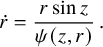 $$ \begin{align} &\hspace{-5pt}\dot r=\frac{r\sin z}{\psi(z,r)}\,. \end{align} $$
Hence, the unperturbed system is Hamiltonian with symplectic form $\omega :=r^{-1}dz\wedge dr$
and Hamiltonian function
$\omega :=r^{-1}dz\wedge dr$
and Hamiltonian function $H(z,r):=\log \psi (z,r)$
. The periodic orbits
$H(z,r):=\log \psi (z,r)$
. The periodic orbits $\gamma _{\pm }$
of v and their heteroclinic cycle
$\gamma _{\pm }$
of v and their heteroclinic cycle $\Gamma _1\cup \Gamma _2$
correspond to the (hyperbolic) fixed points
$\Gamma _1\cup \Gamma _2$
correspond to the (hyperbolic) fixed points $p_{\pm }$
of the unperturbed system joined by two heteroclinic connections
$p_{\pm }$
of the unperturbed system joined by two heteroclinic connections $\widetilde \Gamma _k:=\Gamma _k\cap \{\theta =0\}$
,
$\widetilde \Gamma _k:=\Gamma _k\cap \{\theta =0\}$
, $k=1,2$
. These are precisely the two pieces of the level curve
$k=1,2$
. These are precisely the two pieces of the level curve $\{H(z,r)=\log c_0\}$
that are contained in
$\{H(z,r)=\log c_0\}$
that are contained in ${\mathcal {D}}$
. Let us denote by
${\mathcal {D}}$
. Let us denote by
 $$ \begin{align*}\gamma_k(t)=(Z_k(t;0,r_k),R_k(t;0,r_k))\end{align*} $$
the integral curves of the separatrices that solve equations (5.5) and (5.6) with initial conditions $(0,r_k)\in \widetilde \Gamma _k$
. Of course, the closure of the set
$(0,r_k)\in \widetilde \Gamma _k$
. Of course, the closure of the set ${\{\gamma _k(t):t\in {\mathbb {R}}\}}$
is
${\{\gamma _k(t):t\in {\mathbb {R}}\}}$
is $\widetilde \Gamma _k$
, and the stability analysis of the periodic integral curves
$\widetilde \Gamma _k$
, and the stability analysis of the periodic integral curves $\gamma _{\pm }$
readily implies that
$\gamma _{\pm }$
readily implies that $\lim _{t\to \pm (-1)^{k+1}\infty }\gamma _k(t)=p_{\pm }$
.
$\lim _{t\to \pm (-1)^{k+1}\infty }\gamma _k(t)=p_{\pm }$
.
By the implicit function theorem, the perturbed system (5.3) and (5.4) has exactly two hyperbolic fixed points $p_{\pm }^{\varepsilon }\in {\mathcal {D}}$
so that
$p_{\pm }^{\varepsilon }\in {\mathcal {D}}$
so that $p_{\pm }^{\varepsilon } \to p_{\pm }$
as
$p_{\pm }^{\varepsilon } \to p_{\pm }$
as $\varepsilon \to 0$
. The technical tool to prove that the unstable (resp. stable) manifold of
$\varepsilon \to 0$
. The technical tool to prove that the unstable (resp. stable) manifold of $p_+^{\varepsilon }$
and the stable (resp. unstable) manifold of
$p_+^{\varepsilon }$
and the stable (resp. unstable) manifold of $p_-^{\varepsilon }$
intersect transversely when
$p_-^{\varepsilon }$
intersect transversely when $\varepsilon>0$
is small is the Melnikov function. We define the vector fields
$\varepsilon>0$
is small is the Melnikov function. We define the vector fields $Y_0$
,
$Y_0$
, $Y_1$
, respectively, as the unperturbed system and the first order in
$Y_1$
, respectively, as the unperturbed system and the first order in $\varepsilon $
perturbation, that is,
$\varepsilon $
perturbation, that is,
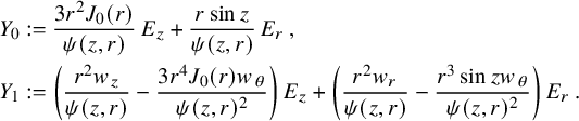 $$ \begin{align*} &Y_0:= \frac{3r^2J_0(r)}{\psi(z,r)}\,E_z+\frac{r\sin z}{\psi(z,r)}\,E_r\,,\\ &Y_1:= \left(\frac{r^2w_z}{\psi(z,r)}-\frac{3r^4J_0(r)w_{\theta}}{\psi(z,r)^2}\right)\,E_z+\left(\frac{r^2w_r}{\psi(z,r)}-\frac{r^3\sin z w_{\theta}}{\psi(z,r)^2}\right)\,E_r\,. \end{align*} $$
Since the unperturbed system is Hamiltonian, we can apply Lemma 5.4 below (which is a variation on known results in Melnikov theory) to conclude that if the Melnikov functions
 $$ \begin{align} M_k(t_0):=\int_{-\infty}^{\infty} \omega(Y_0,Y_1)|_{\gamma_k(t-t_0)}\, dt\, \end{align} $$
have simple zeros for each $k=1,2$
, then the aforementioned transverse intersections exist, and that actually the heteroclinic connections intersect at infinitely many points. The integrand
$k=1,2$
, then the aforementioned transverse intersections exist, and that actually the heteroclinic connections intersect at infinitely many points. The integrand $\omega (Y_0,Y_1)$
denotes the action of the symplectic 2-form
$\omega (Y_0,Y_1)$
denotes the action of the symplectic 2-form $\omega $
on the vector fields
$\omega $
on the vector fields $Y_0,Y_1$
, evaluated on the integral curve
$Y_0,Y_1$
, evaluated on the integral curve $\gamma _k(t-t_0)$
. It is standard that the improper integral in the definition of the Melnikov functions is absolutely convergent because of the hyperbolicity of the fixed points joined by the separatrices (see, e.g., [Reference Guckenheimer and Holmes22, Section 4.5]). Also, notice that although [Reference Guckenheimer and Holmes22, Section 4.5] concerns transverse intersections of homoclinic connections, the analysis applies verbatim to transverse intersections of heteroclinic connections.
$\gamma _k(t-t_0)$
. It is standard that the improper integral in the definition of the Melnikov functions is absolutely convergent because of the hyperbolicity of the fixed points joined by the separatrices (see, e.g., [Reference Guckenheimer and Holmes22, Section 4.5]). Also, notice that although [Reference Guckenheimer and Holmes22, Section 4.5] concerns transverse intersections of homoclinic connections, the analysis applies verbatim to transverse intersections of heteroclinic connections.
More explicitly, the Melnikov functions are given by
 $$\begin{align*}M_k(t_0)=\frac1{c_0^2}\int_{-\infty}^{\infty} R_k(t)^2\big[w_z(Z_k(t),R_k(t),t)\sin Z_k(t)-3R_k(t)J_0(R_k(t))w_r(Z_k(t),R_k(t),t)\big]\,dt\,, \end{align*}$$
where $R_k(t)\equiv R_k(t;0,r_k)$
and
$R_k(t)\equiv R_k(t;0,r_k)$
and $Z_k(t)\equiv Z_k(t;0,r_k)$
. It is well known that the existence of transverse intersections is independent of the choice of initial condition.
$Z_k(t)\equiv Z_k(t;0,r_k)$
. It is well known that the existence of transverse intersections is independent of the choice of initial condition.
To analyze these Melnikov integrals, let us now choose the particular perturbation
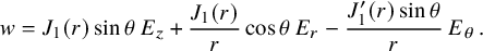 $$ \begin{align} w=J_1(r)\sin \theta\, E_z+\frac{J_1(r)}{r}\cos \theta\, E_r-\frac{J_1'(r)\sin\theta}{r}\,E_{\theta}\,. \end{align} $$
It is easy to check that $\operatorname {\mathrm {curl}} w=w$
in
$\operatorname {\mathrm {curl}} w=w$
in ${\mathbb {R}}^3$
; in fact
${\mathbb {R}}^3$
; in fact $w=(\operatorname {\mathrm {curl}}\operatorname {\mathrm {curl}} +\operatorname {\mathrm {curl}})(J_0(r),0,0)$
(or, to put it differently,
$w=(\operatorname {\mathrm {curl}}\operatorname {\mathrm {curl}} +\operatorname {\mathrm {curl}})(J_0(r),0,0)$
(or, to put it differently, $w=U_{\varphi ' q(\xi _1)^{-1} p}$
, where the distribution
$w=U_{\varphi ' q(\xi _1)^{-1} p}$
, where the distribution $\varphi '$
on the sphere
$\varphi '$
on the sphere ${\mathbb {S}}$
is the Lebesgue measure of the equator, normalized to unit mass). With this choice, the Melnikov functions take the form
${\mathbb {S}}$
is the Lebesgue measure of the equator, normalized to unit mass). With this choice, the Melnikov functions take the form
 $$ \begin{align*} c_0^2M_k(t_0)&=\int_{-\infty}^{\infty} R_k(t)^2\big[J_1(R_k(t))\sin Z_k(t)\sin (t+t_0)-3J_0(R_k(t))J_1(R_k(t))\cos (t+t_0)\big]\,dt \\ &=: a_k\sin t_0 +b_k \cos t_0\,, \end{align*} $$
where the constants $a_k,b_k$
are given by the integrals
$a_k,b_k$
are given by the integrals
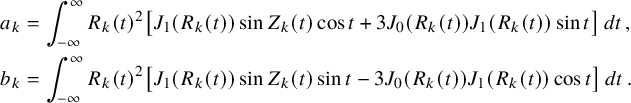 $$ \begin{align*} a_k&=\int_{-\infty}^{\infty} R_k(t)^2\big[J_1(R_k(t))\sin Z_k(t)\cos t+3J_0(R_k(t))J_1(R_k(t))\sin t\big]\,dt\,,\\ b_k&=\int_{-\infty}^{\infty} R_k(t)^2\big[J_1(R_k(t))\sin Z_k(t)\sin t-3J_0(R_k(t))J_1(R_k(t))\cos t\big]\,dt\,. \end{align*} $$
Since the Hamiltonian function has the symmetry $H(-z,r)=H(z,r)$
, it follows that
$H(-z,r)=H(z,r)$
, it follows that $R_k(t)=R_k(-t)$
and
$R_k(t)=R_k(-t)$
and $Z_k(t)=-Z_k(-t)$
. This immediately yields that
$Z_k(t)=-Z_k(-t)$
. This immediately yields that $a_1=a_2=0$
. Moreover, it is not hard to compute the constants
$a_1=a_2=0$
. Moreover, it is not hard to compute the constants $b_1$
and
$b_1$
and $b_2$
numerically:
$b_2$
numerically:
 $$\begin{align*}\quad b_1=3.5508\dots\,,\quad b_2=0.2497\dots \end{align*}$$
Therefore, the function $M_k(t_0)=b_k\cos t_0$
is a nonzero multiple of the cosine, so it obviously has exactly two zeros in the interval
$M_k(t_0)=b_k\cos t_0$
is a nonzero multiple of the cosine, so it obviously has exactly two zeros in the interval $[0,2\pi )$
, which are nondegenerate. It then follows from Lemma 5.4 below that the two heteroclinic connections joining
$[0,2\pi )$
, which are nondegenerate. It then follows from Lemma 5.4 below that the two heteroclinic connections joining $p_{\pm }^{\varepsilon }$
intersect transversely. In turn, this implies [Reference Wiggins33, Theorem 26.1.3] that each hyperbolic fixed point
$p_{\pm }^{\varepsilon }$
intersect transversely. In turn, this implies [Reference Wiggins33, Theorem 26.1.3] that each hyperbolic fixed point $p_{\pm }^{\varepsilon }$
has transverse homoclinic intersections, so by the Birkhoff–Smale theorem [Reference Guckenheimer and Holmes22, Theorem 5.3.5] the perturbed system (5.3) and (5.4) (with w given by equation (5.8)) has a compact hyperbolic invariant set on which the dynamics is topologically conjugate to a Bernoulli shift. This set is contained in a neighborhood of the heteroclinic cycle
$p_{\pm }^{\varepsilon }$
has transverse homoclinic intersections, so by the Birkhoff–Smale theorem [Reference Guckenheimer and Holmes22, Theorem 5.3.5] the perturbed system (5.3) and (5.4) (with w given by equation (5.8)) has a compact hyperbolic invariant set on which the dynamics is topologically conjugate to a Bernoulli shift. This set is contained in a neighborhood of the heteroclinic cycle $\widetilde \Gamma _1 \cup \widetilde \Gamma _2$
, and hence in the planar domain
$\widetilde \Gamma _1 \cup \widetilde \Gamma _2$
, and hence in the planar domain ${\mathcal {D}}$
where the system is defined. This immediately implies that the vector field Y defined in equation (5.2), which is the suspension of the nonautonomous planar system (5.3), has a compact normally hyperbolic invariant set K on which its time-T flow is topologically conjugate to a Bernoulli shift, where
${\mathcal {D}}$
where the system is defined. This immediately implies that the vector field Y defined in equation (5.2), which is the suspension of the nonautonomous planar system (5.3), has a compact normally hyperbolic invariant set K on which its time-T flow is topologically conjugate to a Bernoulli shift, where $T:= 2\pi N$
for some positive integer
$T:= 2\pi N$
for some positive integer $N>0$
. The invariant set K is contained in
$N>0$
. The invariant set K is contained in $\Omega $
because it lies in a small neighborhood of the invariant set
$\Omega $
because it lies in a small neighborhood of the invariant set $\Gamma _1\cup \Gamma _2$
. Since the integral curves of X and Y are the same, up to a reparametrization, K is also a chaotic invariant set of the Beltrami field X in
$\Gamma _1\cup \Gamma _2$
. Since the integral curves of X and Y are the same, up to a reparametrization, K is also a chaotic invariant set of the Beltrami field X in $\Omega $
.
$\Omega $
.
Finally, since ${\mathbb {R}}^3\backslash \overline \Omega $
is connected, and of course the vector field X satisfies the Beltrami equation in an open neighborhood of
${\mathbb {R}}^3\backslash \overline \Omega $
is connected, and of course the vector field X satisfies the Beltrami equation in an open neighborhood of $\overline \Omega $
, for each
$\overline \Omega $
, for each $\delta>0$
, Proposition 2.5 shows that there is a Hermitian finite linear combination of spherical harmonics
$\delta>0$
, Proposition 2.5 shows that there is a Hermitian finite linear combination of spherical harmonics $\varphi $
such that
$\varphi $
such that
 $$\begin{align*}\|X-U_{\varphi p}\|_{C^1(\Omega)}<\delta\,. \end{align*}$$
If $\delta $
is small enough, the stability of transverse intersections implies that the Beltrami field
$\delta $
is small enough, the stability of transverse intersections implies that the Beltrami field $U_{\varphi p}$
has a compact chaotic invariant set
$U_{\varphi p}$
has a compact chaotic invariant set $K_{\delta }$
in a small neighborhood of K on which a suitable reparametrization of its time-T flow is conjugate to a Bernoulli shift, so the proposition follows.
$K_{\delta }$
in a small neighborhood of K on which a suitable reparametrization of its time-T flow is conjugate to a Bernoulli shift, so the proposition follows.
Corollary 5.3. There exists $R_0>0$
and
$R_0>0$
and $\delta>0$
such that
$\delta>0$
such that $N^{\mathrm {h}}_w(R_0)\geqslant 1$
for any vector field w such that
$N^{\mathrm {h}}_w(R_0)\geqslant 1$
for any vector field w such that $\|w-u_0\|_{C^k(B_{R_0})}<\delta $
, provided that
$\|w-u_0\|_{C^k(B_{R_0})}<\delta $
, provided that $k\geqslant 1$
.
$k\geqslant 1$
.
Proof. Taking $R_0$
so that the horseshoe of
$R_0$
so that the horseshoe of $u_0$
is contained in
$u_0$
is contained in $B_{R_0}$
, the result is a straightforward consequence of the lower semicontinuity of
$B_{R_0}$
, the result is a straightforward consequence of the lower semicontinuity of $N^{\mathrm {h}}_u(R)$
, cf. Proposition 5.1.
$N^{\mathrm {h}}_u(R)$
, cf. Proposition 5.1.
To conclude, the following lemma gives the formula for the Melnikov function that we employed in the proof of Proposition 5.2 above. This is an expression for the Melnikov function of perturbations of a planar system that is Hamiltonian with respect to an arbitrary symplectic form. This is a minor generalization of the well-known formulas [Reference Guckenheimer and Holmes22, Theorem 4.5.3] and [Reference Holmes25, Equation (23)], which assume that the symplectic form is the standard one.
Lemma 5.4. Let $Y_0$
be a smooth Hamiltonian vector field defined on a domain
$Y_0$
be a smooth Hamiltonian vector field defined on a domain ${\mathcal {D}}\subset {\mathbb {R}}^2$
with Hamiltonian function H and symplectic form
${\mathcal {D}}\subset {\mathbb {R}}^2$
with Hamiltonian function H and symplectic form $\omega $
. Assume that this system has two hyperbolic fixed points
$\omega $
. Assume that this system has two hyperbolic fixed points $p_{\pm }$
joined by a heteroclinic connection
$p_{\pm }$
joined by a heteroclinic connection $\widetilde \Gamma $
. Take a smooth nonautonomous planar field
$\widetilde \Gamma $
. Take a smooth nonautonomous planar field $Y_1$
, which we assume
$Y_1$
, which we assume $2\pi $
-periodic in time, and consider the perturbed system
$2\pi $
-periodic in time, and consider the perturbed system $Y_0+\varepsilon Y_1+O(\varepsilon ^2)$
. Then the simple zeros of the Melnikov function
$Y_0+\varepsilon Y_1+O(\varepsilon ^2)$
. Then the simple zeros of the Melnikov function
 $$\begin{align*}M(t_0):=\int_{-\infty}^{\infty} \omega(Y_0,Y_1)|_{\gamma(t-t_0;p_0)}\, dt\,, \end{align*}$$
where the integrand is evaluated at the integral curve $\gamma (t-t_0;p_0)$
of
$\gamma (t-t_0;p_0)$
of $Y_0$
parametrizing the separatrix
$Y_0$
parametrizing the separatrix $\widetilde \Gamma $
, give rise to a transverse heteroclinic intersection of the perturbed system, for any small enough
$\widetilde \Gamma $
, give rise to a transverse heteroclinic intersection of the perturbed system, for any small enough $\varepsilon $
.
$\varepsilon $
.
Proof. If $\varepsilon $
is small enough, the perturbed system has two hyperbolic fixed points
$\varepsilon $
is small enough, the perturbed system has two hyperbolic fixed points $p_{\pm }^{\varepsilon }$
. To analyze how the heteroclinic connection is perturbed, we take a point
$p_{\pm }^{\varepsilon }$
. To analyze how the heteroclinic connection is perturbed, we take a point $p_0\in \widetilde \Gamma $
and we compute the so-called displacement (or distance) function
$p_0\in \widetilde \Gamma $
and we compute the so-called displacement (or distance) function $\Delta (t_0)$
on a section
$\Delta (t_0)$
on a section $\Sigma $
based at
$\Sigma $
based at $p_0$
and transverse to
$p_0$
and transverse to $\widetilde \Gamma $
. Recall that the function
$\widetilde \Gamma $
. Recall that the function $\varepsilon \Delta (t_0)$
gives the distance of the splitting, up to order
$\varepsilon \Delta (t_0)$
gives the distance of the splitting, up to order $O(\varepsilon ^2)$
, between the corresponding stable and unstable manifolds of the perturbed system at the section
$O(\varepsilon ^2)$
, between the corresponding stable and unstable manifolds of the perturbed system at the section $\Sigma $
.
$\Sigma $
.
A standard analysis, cf. [Reference Holmes25, Equation (22)] or the proof of [Reference Guckenheimer and Holmes22, Theorem 4.5.3], yields the following formula for $\Delta (t_0)$
:
$\Delta (t_0)$
:
 $$ \begin{align} \Delta(t_0)=\frac{1}{|Y_0(p_0)|}\,\int_{-\infty}^{\infty} Y_1(\gamma(t-t_0))\times Y_0(\gamma(t-t_0)) e^{-\int_0^{t-t_0}\text{Tr}\, DY_0(\gamma(s))\,ds}\,dt\,, \end{align} $$
where we have omitted the dependence of the integral curve on the initial condition $p_0\in \widetilde \Gamma $
. Here, we are using the notation
$p_0\in \widetilde \Gamma $
. Here, we are using the notation $X\times Y:= X_1Y_2-X_2Y_1$
for vectors
$X\times Y:= X_1Y_2-X_2Y_1$
for vectors $X,Y\in {\mathbb {R}}^2$
and
$X,Y\in {\mathbb {R}}^2$
and $\text {Tr}\, DY_0$
is the trace of the Jacobian matrix of the unperturbed field
$\text {Tr}\, DY_0$
is the trace of the Jacobian matrix of the unperturbed field $Y_0$
.
$Y_0$
.
Take coordinates in ${\mathcal {D}}$
, which we will call
${\mathcal {D}}$
, which we will call $(z,r)$
just as in the proof of Proposition 5.2, and write the symplectic form as
$(z,r)$
just as in the proof of Proposition 5.2, and write the symplectic form as $\omega =\rho (z,r)\,dz\wedge dr$
, where
$\omega =\rho (z,r)\,dz\wedge dr$
, where $\rho (z,r)$
is a smooth function that does not vanish. Let us call here
$\rho (z,r)$
is a smooth function that does not vanish. Let us call here $\{e_z,e_r\}$
the basis of vector fields dual to
$\{e_z,e_r\}$
the basis of vector fields dual to $\{dz,dr\}$
(which are usually denoted by
$\{dz,dr\}$
(which are usually denoted by ${\partial }_z$
and
${\partial }_z$
and ${\partial }_r$
, as they correspond to the partial derivatives with respect to the coordinates z and r). The Hamiltonian field
${\partial }_r$
, as they correspond to the partial derivatives with respect to the coordinates z and r). The Hamiltonian field $Y_0$
reads in these coordinates as
$Y_0$
reads in these coordinates as
 $$ \begin{align*}Y_0=\frac{1}{\rho(z,r)}\Big(\partial_r H\, e_z-\partial_zH\, e_r\Big)\,. \end{align*} $$
Noting that
 $$\begin{align*}Y_1(\gamma(t-t_0))\times Y_0(\gamma(t-t_0))=\frac{\omega(Y_0,Y_1)|_{\gamma(t-t_0)}}{\rho(\gamma(t-t_0))} \end{align*}$$
and
 $$ \begin{align} e^{-\int_0^{t-t_0}\text{Tr}\, DY_0(\gamma(s))\,ds}&=e^{\int_{0}^{t-t_0}Y_0(\gamma(s))\cdot \nabla \log \rho(\gamma(s))\,ds}\end{align} $$
 $$ \begin{align}&=e^{\int_0^{t-t_0}\frac{d\log \rho(\gamma(s))}{ds}\,ds}=\frac{\rho(\gamma(t-t_0))}{\rho(p_0)}\,, \end{align} $$
equation (5.9) implies that
 $$\begin{align*}\Delta(t_0)=\frac{M(t_0)}{|Y_0(p_0)|\rho(p_0)}\,, \end{align*}$$
so the claim follows because $M(t_0)$
coincides with the displacement function up to a constant proportionality factor.
$M(t_0)$
coincides with the displacement function up to a constant proportionality factor.
6 Asymptotics for random Beltrami fields on
${\mathbb {R}}^3$

We are now ready to prove our main results about random Beltrami fields on ${\mathbb {R}}^3$
, Theorems 1.2 and 1.5. To do this, as we saw in the two previous sections, we need to handle sets that have a rather geometrically complicated structure, which gives rise to several measurability issues. For this reason, we start this section by proving a version of the Nazarov–Sodin sandwich estimate [Reference Nazarov and Sodin30, Lemma 1] that circumvents some of these issues and which is suitable for our purposes.
${\mathbb {R}}^3$
, Theorems 1.2 and 1.5. To do this, as we saw in the two previous sections, we need to handle sets that have a rather geometrically complicated structure, which gives rise to several measurability issues. For this reason, we start this section by proving a version of the Nazarov–Sodin sandwich estimate [Reference Nazarov and Sodin30, Lemma 1] that circumvents some of these issues and which is suitable for our purposes.
6.1 A sandwich estimate for sets of points and for arbitrary closed sets
For any subset $\Gamma \subset {\mathbb {R}}^3$
, we denote by
$\Gamma \subset {\mathbb {R}}^3$
, we denote by $N(x,r;\Gamma )$
the number of connected components of
$N(x,r;\Gamma )$
the number of connected components of $\Gamma $
that are contained in the ball
$\Gamma $
that are contained in the ball $B_r(x)$
. Also, if
$B_r(x)$
. Also, if ${\mathcal {X}}:=\{ x_j:j\in {\mathcal {J}}\}$
, where
${\mathcal {X}}:=\{ x_j:j\in {\mathcal {J}}\}$
, where $x_j\in {\mathbb {R}}^3$
, is a countable set of points (which is not necessarily a closed subset of
$x_j\in {\mathbb {R}}^3$
, is a countable set of points (which is not necessarily a closed subset of ${\mathbb {R}}^3$
), then we define
${\mathbb {R}}^3$
), then we define
 $$\begin{align*}{\mathcal{N}}(x,r;{\mathcal{X}}):=\#[{\mathcal{X}}\cap B_r(x)] \end{align*}$$
as the number of points of ${\mathcal {X}}$
contained in the open ball
${\mathcal {X}}$
contained in the open ball $B_r(x)$
. For the ease of notation, we will write
$B_r(x)$
. For the ease of notation, we will write $N(r;\Gamma ):=N(0,r;\Gamma )$
and similarly
$N(r;\Gamma ):=N(0,r;\Gamma )$
and similarly ${\mathcal {N}}(r;{\mathcal {X}})$
. We remark that these numbers may be infinite.
${\mathcal {N}}(r;{\mathcal {X}})$
. We remark that these numbers may be infinite.
Lemma 6.1. Let $\Gamma $
be any subset of
$\Gamma $
be any subset of ${\mathbb {R}}^3$
whose connected components are all closed and let
${\mathbb {R}}^3$
whose connected components are all closed and let ${\mathcal {X}}:=\{ x_j:j\in {\mathcal {J}}\}$
, with
${\mathcal {X}}:=\{ x_j:j\in {\mathcal {J}}\}$
, with $x_j\in {\mathbb {R}}^3$
, be a countable set of points of
$x_j\in {\mathbb {R}}^3$
, be a countable set of points of ${\mathbb {R}}^3$
. Then the functions
${\mathbb {R}}^3$
. Then the functions ${\mathcal {N}}(\cdot ,r; {\mathcal {X}})$
and
${\mathcal {N}}(\cdot ,r; {\mathcal {X}})$
and $N(\cdot ,r; \Gamma )$
are measurable, and for any
$N(\cdot ,r; \Gamma )$
are measurable, and for any $0<r<R$
one has
$0<r<R$
one has
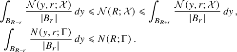 $$ \begin{align*} \int_{B_{R-r}} \frac{{\mathcal{N}}(y, r; {\mathcal{X}})}{ |B_r|}\, {d}y &\leqslant {\mathcal{N}}(R; {\mathcal{X}}) \leqslant \int_{B_{R+r}} \frac{{\mathcal{N}}(y, r; {\mathcal{X}})}{|B_r|}\, {d}y\,,\\ \int_{B_{R-r}} \frac{N(y, r; \Gamma)}{|B_r|}\, dy &\leqslant N(R; \Gamma) \,. \end{align*} $$
Proof. Let us start by noticing that
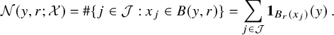 $$\begin{align*}{\mathcal{N}}(y,r;{\mathcal{X}})=\#\lbrace j\in{\mathcal{J}}: x_j\in{B(y,r)} \rbrace= \sum_{j\in{\mathcal{J}}}\mathbf{1}_{{B_r(x_j)}}(y)\,. \end{align*}$$
As the ball ${B_r(x)}$
is an open set, it is clear that
${B_r(x)}$
is an open set, it is clear that $\mathbf {1}_{{B_r(x)}}(\cdot )$
is a lower semicontinuous function. Recall that lower semicontinuity is preserved under sums and that the supremum of an arbitrary set (not necessarily countable) of lower semicontinuous functions is also lower semicontinuous. Therefore, from the formula
$\mathbf {1}_{{B_r(x)}}(\cdot )$
is a lower semicontinuous function. Recall that lower semicontinuity is preserved under sums and that the supremum of an arbitrary set (not necessarily countable) of lower semicontinuous functions is also lower semicontinuous. Therefore, from the formula
 $$ \begin{align*} {\mathcal{N}}(\cdot,r;{\mathcal{X}})=\sup_{{\mathcal{J}}'} \sum_{j\in{\mathcal{J}}'}\mathbf{1}_{{B_r(x_j)}}(\cdot)\,, \end{align*} $$
where ${\mathcal {J}}'$
ranges over all finite subsets of
${\mathcal {J}}'$
ranges over all finite subsets of ${\mathcal {J}}$
, we deduce that the function
${\mathcal {J}}$
, we deduce that the function ${\mathcal {N}}(\cdot ,r;{\mathcal {X}})$
is lower semicontinuous, and therefore measurable.
${\mathcal {N}}(\cdot ,r;{\mathcal {X}})$
is lower semicontinuous, and therefore measurable.
Now, let ${\mathcal {J}}_R:=\{j\in {\mathcal {J}}: x_j\in B_R\}$
and note that
${\mathcal {J}}_R:=\{j\in {\mathcal {J}}: x_j\in B_R\}$
and note that
 $$ \begin{align*} |B_r| {\mathcal{N}}(R; {\mathcal{X}})=\sum_{j\in{\mathcal{J}}_R}\int_{B_{R+r}}\mathbf{1}_{{B_r(x_j)}}(y)\, { d}y\,. \end{align*} $$
As we can interchange the sum and the integral by the monotone convergence theorem and
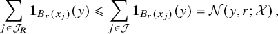 $$ \begin{align*}\sum_{j\in{\mathcal{J}}_R}\mathbf{1}_{{B_r(x_j)}}(y)\leqslant \sum_{j\in{\mathcal{J}}}\mathbf{1}_{{B_r(x_j)}}(y)={\mathcal{N}}(y,r;{\mathcal{X}})\,,\end{align*} $$
one immediately obtains the upper bound for ${\mathcal {N}}(R;{\mathcal {X}})$
. Likewise, using now that
${\mathcal {N}}(R;{\mathcal {X}})$
. Likewise, using now that
 $$ \begin{align*} |B_r| {\mathcal{N}}(R; {\mathcal{X}})&= \sum_{j\in{\mathcal{J}}_R}\int_{B_{R+r}}\mathbf{1}_{{B_r(x_j)}}(y)\,dy\\ &\geqslant\sum_{j\in{\mathcal{J}}_R}\int_{B_{R-r}}\mathbf{1}_{{B_r(x_j)}}(y)\, { d}y\\ &=\sum_{j\in{\mathcal{J}}}\int_{B_{R-r}}\mathbf{1}_{{B_r(x_j)}}(y)\, { d}y =\int_{B_{R-r}}{\mathcal{N}}(y,r;{\mathcal{X}})\, { d}y\,, \end{align*} $$
we derive the lower bound. The sandwich estimate for ${\mathcal {N}}(R;{\mathcal {X}})$
is then proved.
${\mathcal {N}}(R;{\mathcal {X}})$
is then proved.
Now, let $\gamma $
be a connected component of
$\gamma $
be a connected component of $\Gamma $
, which is a closed set by hypothesis. Since
$\Gamma $
, which is a closed set by hypothesis. Since $\gamma \subset B_r(y)$
if and only if
$\gamma \subset B_r(y)$
if and only if $y\in B_r(x)$
for all
$y\in B_r(x)$
for all $x\in \gamma $
, one has that
$x\in \gamma $
, one has that
 $$ \begin{align} N(y,r;\Gamma)=\sum_{\gamma\subset \Gamma}\mathbf{1}_{\gamma^r}(y)\,, \end{align} $$
where the sum is over the connected components of $\Gamma $
and the set
$\Gamma $
and the set $\gamma ^r$
is defined, for each connected component
$\gamma ^r$
is defined, for each connected component $\gamma $
of
$\gamma $
of $\Gamma $
, as
$\Gamma $
, as
 $$\begin{align*}\gamma^r:=\bigcap_{x\in\gamma}B_r(x)\,, \end{align*}$$
that is, as the set of points in $\mathbb R^3$
whose distance to any point of
$\mathbb R^3$
whose distance to any point of $\gamma $
is less than r. Obviously, the set
$\gamma $
is less than r. Obviously, the set $\gamma ^r$
is open, so
$\gamma ^r$
is open, so $\mathbf {1}_{\gamma ^r}$
is lower semicontinuous and contained in the ball
$\mathbf {1}_{\gamma ^r}$
is lower semicontinuous and contained in the ball $B_r(x_0)$
, where
$B_r(x_0)$
, where $x_0$
is any point of
$x_0$
is any point of $\gamma $
. Also notice that
$\gamma $
. Also notice that $\gamma ^r$
is not the empty set provided that
$\gamma ^r$
is not the empty set provided that $2r$
is larger than the diameter of
$2r$
is larger than the diameter of $\gamma $
. Therefore, by the same argument as before, if follows from the expression (6.1) that the function
$\gamma $
. Therefore, by the same argument as before, if follows from the expression (6.1) that the function $N(\cdot ,r;\Gamma )$
is measurable. If we now define the set
$N(\cdot ,r;\Gamma )$
is measurable. If we now define the set $\Gamma _R$
consisting of the connected components of
$\Gamma _R$
consisting of the connected components of $\Gamma $
that are contained in the ball
$\Gamma $
that are contained in the ball $B_R$
, the same argument as before shows that
$B_R$
, the same argument as before shows that
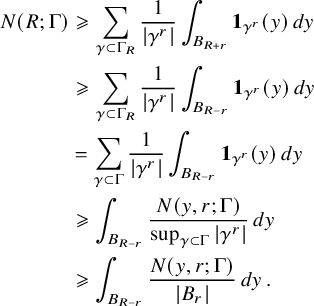 $$ \begin{align*} N(R;\Gamma)&\geqslant \sum_{\gamma\subset \Gamma_R}\frac{1}{|\gamma^r|}\int_{B_{R+r}}\mathbf{1}_{\gamma^r}(y)\, { d}y\\ &\geqslant \sum_{\gamma\subset \Gamma_R}\frac{1}{|\gamma^r|}\int_{B_{R-r}}\mathbf{1}_{\gamma^r}(y)\, { d}y\\ &=\sum_{\gamma\subset \Gamma}\frac{1}{|\gamma^r|}\int_{B_{R-r}}\mathbf{1}_{\gamma^r}(y)\, { d}y\\ &\geqslant\int_{B_{R-r}} \frac{N(y,r;\Gamma)}{\sup_{\gamma\subset \Gamma}|\gamma^r|}\, dy\\ &\geqslant \int_{B_{R-r}} \frac{N(y,r;\Gamma)}{|B_r|}\, dy\,. \end{align*} $$
In the first inequality, we are summing over components $\gamma $
whose diameter is smaller than
$\gamma $
whose diameter is smaller than $2r$
, and to pass to the last inequality we have used the obvious volume bound
$2r$
, and to pass to the last inequality we have used the obvious volume bound $|\gamma ^r|\leqslant |B_r|$
. Note that the proof of the upper bound for
$|\gamma ^r|\leqslant |B_r|$
. Note that the proof of the upper bound for ${\mathcal {N}}(R; {\mathcal {X}})$
does not apply in this case, essentially because we do not have lower bounds for
${\mathcal {N}}(R; {\mathcal {X}})$
does not apply in this case, essentially because we do not have lower bounds for $|\gamma ^r|$
in terms of
$|\gamma ^r|$
in terms of $|B_r|$
.
$|B_r|$
.
6.2 Proof of Theorem 1.2 and Corollary 1.3
We are ready to prove Theorem 1.2. In fact, we will establish a stronger result which permits controlling the parameters of the periodic orbits and the invariant tori. In what follows, we shall use the notation introduced in Sections 4 and 5 for the number of periodic orbits ${N^{\mathrm {o}}_u}(R;[\gamma ],{\mathcal {I}})$
, the number of Diophantine toroidal sets
${N^{\mathrm {o}}_u}(R;[\gamma ],{\mathcal {I}})$
, the number of Diophantine toroidal sets ${N^{\mathrm {t}}_u}(R;[{\mathcal T}],{\mathcal {J}}, V_0)$
(and the volume of the set of invariant tori
${N^{\mathrm {t}}_u}(R;[{\mathcal T}],{\mathcal {J}}, V_0)$
(and the volume of the set of invariant tori ${V^{\mathrm {t}}_u}(R;[{\mathcal T}],{\mathcal {J}})$
) and the number of horseshoes
${V^{\mathrm {t}}_u}(R;[{\mathcal T}],{\mathcal {J}})$
) and the number of horseshoes ${N^{\mathrm {h}}_u}(R)$
. This is useful in itself, since we showed in Section 4.1 that the quantity
${N^{\mathrm {h}}_u}(R)$
. This is useful in itself, since we showed in Section 4.1 that the quantity ${N^{\mathrm {o}}_u}(R;[\gamma ],{\mathcal {I}})$
is finite but this does not need to be the case if one just counts
${N^{\mathrm {o}}_u}(R;[\gamma ],{\mathcal {I}})$
is finite but this does not need to be the case if one just counts ${N^{\mathrm {o}}_u}(R;[\gamma ])$
. Also, the choice of counting the volume of invariant tori instead of its number (which one definitely expect to be infinite) provides the trivial bound
${N^{\mathrm {o}}_u}(R;[\gamma ])$
. Also, the choice of counting the volume of invariant tori instead of its number (which one definitely expect to be infinite) provides the trivial bound ${V^{\mathrm {t}}_u}(R;[{\mathcal T}],{\mathcal {J}})\leqslant |B_R|$
. Specifically, the result we prove is the following.
${V^{\mathrm {t}}_u}(R;[{\mathcal T}],{\mathcal {J}})\leqslant |B_R|$
. Specifically, the result we prove is the following.
Theorem 6.2. Consider a closed curve $\gamma $
and an embedded torus
$\gamma $
and an embedded torus ${\mathcal T}$
of
${\mathcal T}$
of ${\mathbb {R}}^3$
. Then for any
${\mathbb {R}}^3$
. Then for any ${\mathcal {I}}=(T_1,T_2,\Lambda _1,\Lambda _2)$
, some
${\mathcal {I}}=(T_1,T_2,\Lambda _1,\Lambda _2)$
, some ${\mathcal {J}}=(\omega _1,\omega _2,\tau _1,\tau _2)$
and some
${\mathcal {J}}=(\omega _1,\omega _2,\tau _1,\tau _2)$
and some $V_0>0$
, where
$V_0>0$
, where
 $$\begin{align*}0<T_1<T_2\,,\quad 0<\Lambda_1<\Lambda_2\,,\quad 0<\omega_1<\omega_2\,,\quad 0<\tau_1<\tau_2\,, \end{align*}$$
a Gaussian random Beltrami field u satisfies
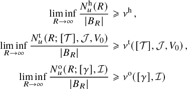 $$ \begin{align*} \liminf_{R\to\infty} \frac{{N^{\mathrm{h}}_u}(R)}{|B_R|}&\geqslant{\nu^{\mathrm{h}}}\,,\\[1mm] \liminf_{R\to\infty} \frac{{N^{\mathrm{t}}_u}(R;[{\mathcal T}],{\mathcal{J}},V_0)}{|B_R|}&\geqslant{\nu^{\mathrm{t}}}([{\mathcal T}],{\mathcal{J}},V_0)\,,\\[1mm] \liminf_{R\to\infty} \frac{{N^{\mathrm{o}}_u}(R;[\gamma],{\mathcal{I}})}{|B_R|}&\geqslant{\nu^{\mathrm{o}}}([\gamma],{\mathcal{I}}) \end{align*} $$
with probability $1$
, with constants that are all positive. In particular, the topological entropy of u is positive almost surely, and
$1$
, with constants that are all positive. In particular, the topological entropy of u is positive almost surely, and
 $$\begin{align*}\liminf_{R\to\infty} \frac{{V^{\mathrm{t}}_u}(R;[{\mathcal T}],{\mathcal{J}})}{|B_R|}\geqslant V_0\,{\nu^{\mathrm{t}}}([{\mathcal T}],{\mathcal{J}},V_0)\,, \end{align*}$$
with probability $1$
.
$1$
.
Proof. For the ease of notation, let us denote by $\Phi _R(u)$
the quantities
$\Phi _R(u)$
the quantities ${N^{\mathrm {h}}_u}(R)$
,
${N^{\mathrm {h}}_u}(R)$
, ${N^{\mathrm {o}}_u}(R;[\gamma ],{\mathcal {I}})$
and
${N^{\mathrm {o}}_u}(R;[\gamma ],{\mathcal {I}})$
and ${N^{\mathrm {t}}_u}(R;[{\mathcal T}],{\mathcal {J}},V_0)$
, in each case. Horseshoes are closed, and so are the set of periodic orbits isotopic to
${N^{\mathrm {t}}_u}(R;[{\mathcal T}],{\mathcal {J}},V_0)$
, in each case. Horseshoes are closed, and so are the set of periodic orbits isotopic to $\gamma $
with parameters in
$\gamma $
with parameters in ${\mathcal {I}}$
and the set of closed invariant solid tori of the kind counted by
${\mathcal {I}}$
and the set of closed invariant solid tori of the kind counted by ${N^{\mathrm {t}}_u}(R;[{\mathcal T}],{\mathcal {J}},V_0)$
. Therefore, the lower bound for sets
${N^{\mathrm {t}}_u}(R;[{\mathcal T}],{\mathcal {J}},V_0)$
. Therefore, the lower bound for sets $\Gamma $
whose components are closed proved in Lemma 6.1 ensures that, for any
$\Gamma $
whose components are closed proved in Lemma 6.1 ensures that, for any $0<r<R$
,
$0<r<R$
,
 $$ \begin{align*} \frac{\Phi_R(u)}{|B_R|}\geqslant \frac1{|B_R|} \int_{B_{R-r}}\frac{\Phi_r(\tau_yu)}{|B_r|}\, dy \geqslant \frac1{|B_R|} \int_{B_{R-r}}\frac{\Phi_r^m(\tau_yu)}{|B_r|}\, dy\,, \end{align*} $$
where for any large $m>1$
we have defined the truncation
$m>1$
we have defined the truncation
 $$\begin{align*}\Phi_r^m(w):= \min\{\Phi_r(w),m\}\,. \end{align*}$$
We recall that the translation operator is defined as $\tau _yu(\cdot )=u(\cdot +y)$
.
$\tau _yu(\cdot )=u(\cdot +y)$
.
As the truncated random variable $\Phi _r^m$
is in
$\Phi _r^m$
is in $L^1(C^k({\mathbb {R}}^3,{\mathbb {R}}^3),\mu _u)$
for any m, one can consider the limit
$L^1(C^k({\mathbb {R}}^3,{\mathbb {R}}^3),\mu _u)$
for any m, one can consider the limit $R\to \infty $
and apply Proposition 3.8 to conclude that
$R\to \infty $
and apply Proposition 3.8 to conclude that
 $\mu _u$
-almost surely, for any r and m. Corollaries 4.3, 4.8 and 5.3 imply that (for any
$\mu _u$
-almost surely, for any r and m. Corollaries 4.3, 4.8 and 5.3 imply that (for any ${\mathcal {I}}$
in the case of periodic orbits, for some
${\mathcal {I}}$
in the case of periodic orbits, for some ${\mathcal {J}}$
and some
${\mathcal {J}}$
and some $V_0>0$
in the case of invariant tori, and unconditionally in the case of horseshoes), there exists some
$V_0>0$
in the case of invariant tori, and unconditionally in the case of horseshoes), there exists some $r>0$
, some
$r>0$
, some $\delta>0$
and a Beltrami field
$\delta>0$
and a Beltrami field $u_0$
such that
$u_0$
such that
 $$\begin{align*}\Phi_r(w)\geqslant 1 \end{align*}$$
for any divergence-free vector field $w\in C^k({\mathbb {R}}^3,{\mathbb {R}}^3)$
with
$w\in C^k({\mathbb {R}}^3,{\mathbb {R}}^3)$
with $\|w-u_0\|_{C^4(B_r)}<\delta $
. As the random variable
$\|w-u_0\|_{C^4(B_r)}<\delta $
. As the random variable $\Phi _r$
is nonnegative, and the measure
$\Phi _r$
is nonnegative, and the measure $\mu _u$
is supported on Beltrami fields (cf. Proposition 3.9), which are divergence-free, it is then immediate that, when picking the parameters
$\mu _u$
is supported on Beltrami fields (cf. Proposition 3.9), which are divergence-free, it is then immediate that, when picking the parameters ${\mathcal {I}}$
,
${\mathcal {I}}$
, ${\mathcal {J}}$
and
${\mathcal {J}}$
and $V_0$
as above, one has for
$V_0$
as above, one has for $k\geqslant 4$
 $$\begin{align*}{\mathbb{E}} \Phi_r^m\geqslant \mu_u\big(\{ w\in C^k({\mathbb{R}}^3,{\mathbb{R}}^3): \|w-u_0\|_{C^k(B_r)}<\delta\}\big)=:\mathcal M(u_0,\delta)\,. \end{align*}$$
This is positive again by Proposition 3.9. So defining the constant, in each case, as
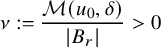 $$ \begin{align*} \nu:=\frac{\mathcal M(u_0,\delta)}{|B_r|}>0 \end{align*} $$
the first part of the theorem follows.
Finally, the topological entropy of u is positive almost surely because u has a horseshoe with probability 1; see Proposition 5.1. The estimate for the growth of the volume of Diophantine invariant tori follows from the trivial lower bound
 $$ \begin{align*}{V^{\mathrm{t}}_u}(R;[{\mathcal T}],{\mathcal{J}})>V_0\,{N^{\mathrm{t}}_u}(R;[{\mathcal T}],{\mathcal{J}},V_0)\,.\\[-34pt]\end{align*} $$
Remark 6.3. A simple variation of the proof of Theorem 6.2 provides an analogous result for links. We recall that a link $\mathcal L$
is a finite set of pairwise disjoint closed curves in
$\mathcal L$
is a finite set of pairwise disjoint closed curves in ${\mathbb {R}}^3$
, which can be knotted and linked among them. More precisely, if
${\mathbb {R}}^3$
, which can be knotted and linked among them. More precisely, if $N^{\mathrm {l}}(R;[\mathcal L],{\mathcal {I}})$
is the number of unions of hyperbolic periodic orbits of u that are contained in
$N^{\mathrm {l}}(R;[\mathcal L],{\mathcal {I}})$
is the number of unions of hyperbolic periodic orbits of u that are contained in $B_R$
, isotopic to the link
$B_R$
, isotopic to the link $\mathcal L$
, and whose periods and maximal Lyapunov exponents are in the intervals prescribed by
$\mathcal L$
, and whose periods and maximal Lyapunov exponents are in the intervals prescribed by ${\mathcal {I}}$
, then
${\mathcal {I}}$
, then
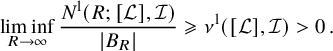 $$\begin{align*}\liminf_{R\to\infty} \frac{N^{\mathrm{l}}(R;[\mathcal L],{\mathcal{I}})}{|B_R|}\geqslant\nu^{\mathrm{l}}([\mathcal L],{\mathcal{I}})>0\,. \end{align*}$$
To apply the lower bound obtained in Lemma 6.1 to estimate the number of links, it is enough to transform each link into a connected set by joining its different components by closed arcs. The proof then goes exactly as in Theorem 6.2 upon noticing that analogs of Proposition 4.2 and Corollary 4.3 also hold for links (the proof easily carries over to this case).
Proof of Corollary 1.3.
The corollary is now an immediate consequence of the fact that the number of isotopy classes of closed curves and embedded tori is countable. Indeed, by Theorem 1.2, with probability 1, a Gaussian random Beltrami field has infinitely many horseshoes, an infinite volume of ergodic invariant tori isotopic to a given embedded torus ${\mathcal T}$
and infinitely many periodic orbits isotopic to a given closed curve
${\mathcal T}$
and infinitely many periodic orbits isotopic to a given closed curve $\gamma $
. Since the countable intersection of sets of probability 1 also has probability
$\gamma $
. Since the countable intersection of sets of probability 1 also has probability $1$
, the claim follows.
$1$
, the claim follows.
6.3 Proof of Theorem 1.5
We are now ready to prove the asymptotics for the number of zeros of the Gaussian random Beltrami field u. Let us start by noticing that, almost surely, the zeros of u are nondegenerate. This is because
 $$\begin{align*}\mu_u\big(\big\{ w\in C^k({\mathbb{R}}^3,{\mathbb{R}}^3): \det\nabla w(x)=0 \;\text{and}\; w(x)=0 \text{ for some } x\in{\mathbb{R}}^3\big\}\big)=0\,, \end{align*}$$
which is a consequence of the boundedness of the probability density function (cf. Remark 3.7) and that u is $C^{\infty }$
almost surely; see [Reference Azais and Wschebor4, Proposition 6.5]. Hence, the intersection of the zero set
$C^{\infty }$
almost surely; see [Reference Azais and Wschebor4, Proposition 6.5]. Hence, the intersection of the zero set
 $$\begin{align*}{\mathcal{X}}_w:=\{x\in{\mathbb{R}}^3: w(x)=0\} \end{align*}$$
with a ball $B_R$
is a finite set of points almost surely. The implicit function theorem then implies that these zeros are robust under
$B_R$
is a finite set of points almost surely. The implicit function theorem then implies that these zeros are robust under $C^1$
-small perturbations so that with probability
$C^1$
-small perturbations so that with probability $1$
,
$1$
, ${\mathcal {N}}(R;{\mathcal {X}}_v)\geqslant {\mathcal {N}}(R;{\mathcal {X}}_w)$
for any vector field v that is close enough to w in the
${\mathcal {N}}(R;{\mathcal {X}}_v)\geqslant {\mathcal {N}}(R;{\mathcal {X}}_w)$
for any vector field v that is close enough to w in the $C^1$
norm. Summarizing, we have the following.
$C^1$
norm. Summarizing, we have the following.
Proposition 6.4. Almost surely, the functional $w\mapsto {\mathcal {N}}(R;{\mathcal {X}}_w)$
is lower semicontinuous in the
$w\mapsto {\mathcal {N}}(R;{\mathcal {X}}_w)$
is lower semicontinuous in the $C^k$
compact open topology for vector fields, for any
$C^k$
compact open topology for vector fields, for any $k\geqslant 1$
. Furthermore,
$k\geqslant 1$
. Furthermore, ${\mathcal {N}}(R;{\mathcal {X}}_w)<\infty $
with probability
${\mathcal {N}}(R;{\mathcal {X}}_w)<\infty $
with probability $1$
.
$1$
.
Since the variance ${\mathbb {E}}[u(x)\otimes u(x)]$
is the identity matrix by Corollary 3.6, the Kac–Rice formula [Reference Azais and Wschebor4, Proposition 6.2] then enables us to compute the expected value of the random variable
${\mathbb {E}}[u(x)\otimes u(x)]$
is the identity matrix by Corollary 3.6, the Kac–Rice formula [Reference Azais and Wschebor4, Proposition 6.2] then enables us to compute the expected value of the random variable
 $$ \begin{align} \Phi_r(w):=\frac{{\mathcal{N}}(r;{\mathcal{X}}_w)}{|B_r|} \end{align} $$
as
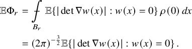
Here, we have used that the above conditional expectation is independent of the point $x\in {\mathbb {R}}^3$
by the translational invariance of the probability measure. We recall that the probability density function
$x\in {\mathbb {R}}^3$
by the translational invariance of the probability measure. We recall that the probability density function $\rho (y):= (2\pi )^{-\frac 32}\, e^{-\frac 12|y|^2}$
was introduced in Remark 3.7.
$\rho (y):= (2\pi )^{-\frac 32}\, e^{-\frac 12|y|^2}$
was introduced in Remark 3.7.
To compute the above conditional expectation value, one can argue as follows.
Lemma 6.5. For any $x\in {\mathbb {R}}^3$
,
$x\in {\mathbb {R}}^3$
,
 $$\begin{align*}{\mathbb{E}}\{ |\det \nabla u(x)| : u(x)=0\}= (2\pi)^{\frac32}{\nu^{\mathrm{z}}}\,, \end{align*}$$
where the constant ${\nu ^{\mathrm {z}}}$
is given by (1.4).
${\nu ^{\mathrm {z}}}$
is given by (1.4).
Proof. Let us first reduce the computation of the conditional expectation to that of an ordinary expectation by introducing a new random variable $\zeta $
. Just like
$\zeta $
. Just like $\nabla u(x)$
, this new variable takes values in the space of
$\nabla u(x)$
, this new variable takes values in the space of $3\times 3$
matrices, which we will identify with
$3\times 3$
matrices, which we will identify with ${\mathbb {R}}^9$
by labeling the matrix entries as
${\mathbb {R}}^9$
by labeling the matrix entries as
 $$ \begin{align} \zeta=: \left( \begin{array}{ccc} \zeta _1 & \zeta _2 & \zeta _3 \\ \zeta _4 & \zeta _5 & \zeta _6 \\ \zeta _7 & \zeta _8 & \zeta _9 \\ \end{array} \right)\,. \end{align} $$
This variable is defined as
 $$ \begin{align} \zeta:= \nabla u(x)-B u(x)\,, \end{align} $$
where the linear operator B (which is a $9\times 3$
matrix if we identify
$9\times 3$
matrix if we identify $\nabla u(x)$
with a vector in
$\nabla u(x)$
with a vector in ${\mathbb {R}}^9$
) is chosen so that the covariance matrix of
${\mathbb {R}}^9$
) is chosen so that the covariance matrix of $u(x)$
and
$u(x)$
and $\zeta $
is 0:
$\zeta $
is 0:
 $$\begin{align*}B:={\mathbb{E}} (\nabla u(x)\otimes u(x))\big[{\mathbb{E}} ( u(x)\otimes u(x))\big]^{-1}={\mathbb{E}} (\nabla u(x)\otimes u(x))\,. \end{align*}$$
Here, we have used that the second matrix is in fact the identity by Corollary 3.6. An easy computation shows that then
 $$\begin{align*}{\mathbb{E}}(\zeta\otimes u(x))=0\,; \end{align*}$$
as $u(x)$
and
$u(x)$
and $\zeta $
are Gaussian vectors with zero mean, this condition ensures that they are independent random variables. Therefore, we can use the identity (6.5) to write the conditional expectation as
$\zeta $
are Gaussian vectors with zero mean, this condition ensures that they are independent random variables. Therefore, we can use the identity (6.5) to write the conditional expectation as
 $$\begin{align*}{\mathbb{E}}\{ |\det \nabla u(x)| : u(x)=0\}= {\mathbb{E}}\{ |\det [\zeta+ Bu(x)]| : u(x)=0\}={\mathbb{E}}|\det\zeta|\,. \end{align*}$$
Our next goal is to compute the covariance matrix of $\zeta $
in closed form, which will enable us to find the expectation of
$\zeta $
in closed form, which will enable us to find the expectation of $|\det \zeta |$
. By definition,
$|\det \zeta |$
. By definition,
 $$ \begin{align*} {\mathbb{E}}(\zeta\otimes \zeta)&= {\mathbb{E}}[(\nabla u(x)-B u(x))\otimes (\nabla u(x)-B u(x))]\\ &={\mathbb{E}}[\nabla u(x)\otimes \nabla u(x)]- {\mathbb{E}}[\nabla u(x)\otimes u(x)]\, {\mathbb{E}}[ u(x) \otimes \nabla u(x)]\,. \end{align*} $$
The basic observation now is that, for any Hermitian polynomials in three variables $q(\xi )$
and
$q(\xi )$
and $q'(\xi )$
, the argument that we used to establish the formula (3.3) and Corollary 3.6 shows that
$q'(\xi )$
, the argument that we used to establish the formula (3.3) and Corollary 3.6 shows that
 $$ \begin{align*} {\mathbb{E}}[(q(D) u_j(x))\, (q'(D)u_k(x))]&= {\mathbb{E}}[q(D_x) u_j(x)\, \overline{q'(D_y)u_k(y)}]|_{y=x}\\ &= \int_{\mathbb{S}} q(\xi)\, q'(-\xi)\, p_j(\xi)\, \overline{p_k(\xi)}\, e^{i\xi\cdot (x-y)}\, d{\sigma}(\xi)\bigg|_{y=x}\\ &= \int_{\mathbb{S}} q(\xi)\, q'(-\xi)\, p_j(\xi)\, \overline{p_k(\xi)}\, d{\sigma}(\xi)\,. \end{align*} $$
Here, we have used that $q'(D)u_k$
is real-valued because
$q'(D)u_k$
is real-valued because $q'$
is Hermitian. As all the matrix integrals in the calculation of
$q'$
is Hermitian. As all the matrix integrals in the calculation of ${\mathbb {E}}(\zeta \otimes \zeta )$
are of this form with
${\mathbb {E}}(\zeta \otimes \zeta )$
are of this form with $q(\xi )=i\xi $
or
$q(\xi )=i\xi $
or $1$
, the computation again boils down to evaluating integrals of the form
$1$
, the computation again boils down to evaluating integrals of the form $\int _{\mathbb {S}} \xi ^{\alpha }\, d{\sigma }(\xi )$
, which can be computed using the formula (3.4).
$\int _{\mathbb {S}} \xi ^{\alpha }\, d{\sigma }(\xi )$
, which can be computed using the formula (3.4).
Tedious but straightforward computations then yield the following explicit formula for the covariance matrix of $\zeta $
:
$\zeta $
:
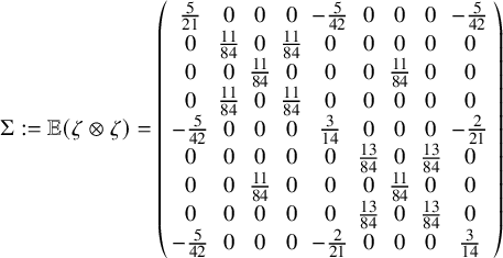 $$\begin{align*}{\Sigma}:= {\mathbb{E}}(\zeta\otimes\zeta)= \left( \begin{array}{ccccccccc} \frac{5}{21} & 0 & 0 & 0 & -\frac{5}{42} & 0 & 0 & 0 & -\frac{5}{42} \\ 0 & \frac{11}{84} & 0 & \frac{11}{84} & 0 & 0 & 0 & 0 & 0 \\ 0 & 0 & \frac{11}{84} & 0 & 0 & 0 & \frac{11}{84} & 0 & 0 \\ 0 & \frac{11}{84} & 0 & \frac{11}{84} & 0 & 0 & 0 & 0 & 0 \\ -\frac{5}{42} & 0 & 0 & 0 & \frac{3}{14} & 0 & 0 & 0 & -\frac{2}{21} \\ 0 & 0 & 0 & 0 & 0 & \frac{13}{84} & 0 & \frac{13}{84} & 0 \\ 0 & 0 & \frac{11}{84} & 0 & 0 & 0 & \frac{11}{84} & 0 & 0 \\ 0 & 0 & 0 & 0 & 0 & \frac{13}{84} & 0 & \frac{13}{84} & 0 \\ -\frac{5}{42} & 0 & 0 & 0 & -\frac{2}{21} & 0 & 0 & 0 & \frac{3}{14} \\ \end{array} \right) \end{align*}$$
Note that this matrix is not invertible: it has rank 5, and an orthogonal basis for the ( $4$
-dimensional) kernel is
$4$
-dimensional) kernel is
 $$ \begin{align*}\{ e_1+e_5+e_9,\; e_2-e_4,\; e_3-e_7, \; e_6-e_8\}\,, \end{align*} $$
where $\{e_j\}_{j=1}^9$
denotes the canonical basis of
$\{e_j\}_{j=1}^9$
denotes the canonical basis of ${\mathbb {R}}^9$
. As we are dealing with Gaussian vectors, this is equivalent to the assertion that
${\mathbb {R}}^9$
. As we are dealing with Gaussian vectors, this is equivalent to the assertion that
 $$ \begin{align} \zeta_1+\zeta_5+\zeta_9=0\,,\quad \zeta_2=\zeta_4\,,\quad \zeta_3=\zeta_7\,,\quad \zeta_6=\zeta_8\ \end{align} $$
almost surely (which amounts to saying that $\zeta $
is a traceless symmetric matrix). Notice that these equations define a
$\zeta $
is a traceless symmetric matrix). Notice that these equations define a $5$
-dimensional subspace orthogonal to the kernel of
$5$
-dimensional subspace orthogonal to the kernel of ${\Sigma }$
. The remaining random variables
${\Sigma }$
. The remaining random variables $\zeta ':= (\zeta _1,\zeta _2,\zeta _3,\zeta _5,\zeta _6)$
are independent Gaussians with zero mean and covariance matrix
$\zeta ':= (\zeta _1,\zeta _2,\zeta _3,\zeta _5,\zeta _6)$
are independent Gaussians with zero mean and covariance matrix
 $$\begin{align*}\Sigma':={\mathbb{E}}(\zeta'\otimes\zeta')=\left( \begin{array}{ccccc} \frac{5}{21} & 0 & 0 & -\frac{5}{42} & 0 \\ 0 & \frac{11}{84} & 0 & 0 & 0 \\ 0 & 0 & \frac{11}{84} & 0 & 0 \\ -\frac{5}{42} & 0 & 0 & \frac{3}{14} & 0 \\ 0 & 0 & 0 & 0 & \frac{13}{84} \\ \end{array} \right) \end{align*}$$
By construction, ${\Sigma }'$
is an invertible matrix, so we can immediately write down a formula for the expectation value of
${\Sigma }'$
is an invertible matrix, so we can immediately write down a formula for the expectation value of $|\det \zeta |$
:
$|\det \zeta |$
:
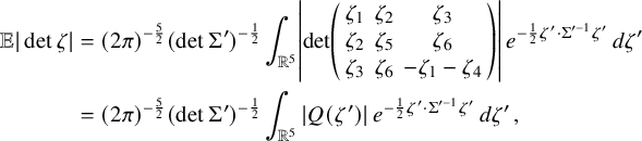 $$ \begin{align*} {\mathbb{E}}|\det\zeta|&=(2\pi)^{-\frac52} (\det{\Sigma}')^{-\frac12}\int_{{\mathbb{R}}^5} \left| \det\left( \begin{array}{ccc} \zeta _1 & \zeta _2 & \zeta _3 \\ \zeta _2 & \zeta _5 & \zeta _6 \\ \zeta _3 & \zeta _6 & -\zeta_1-\zeta_4 \\ \end{array} \right)\right|\, e^{-\frac12\zeta'\cdot {\Sigma}^{\prime -1}\zeta'}\, d\zeta'\\ &=(2\pi)^{-\frac52} (\det{\Sigma}')^{-\frac12}\int_{{\mathbb{R}}^5} | Q(\zeta')|\, e^{-\frac12\zeta'\cdot {\Sigma}^{\prime -1}\zeta'}\, d\zeta'\,, \end{align*} $$
with the cubic polynomial Q being defined as in equation (1.5). Since $\frac 12 \zeta '\cdot {\Sigma }^{\prime -1}\zeta '= \widetilde Q(\zeta ')$
, where the quadratic polynomial
$\frac 12 \zeta '\cdot {\Sigma }^{\prime -1}\zeta '= \widetilde Q(\zeta ')$
, where the quadratic polynomial $\widetilde Q$
was defined in equation (1.6), and
$\widetilde Q$
was defined in equation (1.6), and
 $$\begin{align*}\det{\Sigma}'=\frac{5\cdot 143^2}{{2^8}\cdot{21^5}}\,, \end{align*}$$
we therefore have
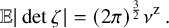 $$\begin{align*}{\mathbb{E}}|\det\zeta|=(2\pi)^{\frac32}{\nu^{\mathrm{z}}}\,. \end{align*}$$
The result then follows.
Remark 6.6. If one keeps track of the connection between $\zeta $
and
$\zeta $
and $\nabla u(x)$
, it is not hard to see that the first condition
$\nabla u(x)$
, it is not hard to see that the first condition $\zeta _1+\zeta _5+\zeta _9=0$
in equation (6.6) is equivalent to
$\zeta _1+\zeta _5+\zeta _9=0$
in equation (6.6) is equivalent to $\operatorname {\mathrm {div}} u(x)=0$
, while the remaining three just mean that
$\operatorname {\mathrm {div}} u(x)=0$
, while the remaining three just mean that $\operatorname {\mathrm {curl}} u(x)= u(x)$
, at the points
$\operatorname {\mathrm {curl}} u(x)= u(x)$
, at the points $x\in {\mathbb {R}}^3$
, where
$x\in {\mathbb {R}}^3$
, where $u(x)=0$
.
$u(x)=0$
.
In particular, this shows that $\Phi _R\in L^1(C^k({\mathbb {R}}^3,{\mathbb {R}}^3),\mu _u)$
. For the ease of notation, let us define the ergodic mean operator
$\Phi _R\in L^1(C^k({\mathbb {R}}^3,{\mathbb {R}}^3),\mu _u)$
. For the ease of notation, let us define the ergodic mean operator
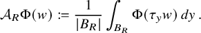 $$\begin{align*}{\mathcal{A}}_R\Phi(w):= \frac1{|B_R|} \int_{B_R} \Phi(\tau_y w)\,{d}y\,. \end{align*}$$
Since ${\mathcal {N}}(R,{\mathcal {X}}_w)$
is finite almost surely, cf. Proposition 6.4, the sandwich estimate proved in Lemma 6.1 implies that, almost surely,
${\mathcal {N}}(R,{\mathcal {X}}_w)$
is finite almost surely, cf. Proposition 6.4, the sandwich estimate proved in Lemma 6.1 implies that, almost surely,
 $$\begin{align*}\frac1{|B_R|}\int_{B_{R-r}}\Phi_r(\tau_yw)\, dy\leqslant \Phi_R(w)\leqslant \frac1{|B_R|}\int_{B_{R+r}}\Phi_r(\tau_yw)\, dy \end{align*}$$
for any $0<r<R$
. Therefore, and using that
$0<r<R$
. Therefore, and using that $|B_{R\pm r}|/|B_R|=(1\pm r/R)^3$
, one has
$|B_{R\pm r}|/|B_R|=(1\pm r/R)^3$
, one has
 $$\begin{align*}|\Phi_R-{\mathcal{A}}_R\Phi_r|\leqslant \bigg|\bigg(1+\frac rR\bigg)^3 {\mathcal{A}}_{R+r}\Phi_r-{\mathcal{A}}_R\Phi_r\bigg| + \bigg|\bigg(1-\frac rR\bigg)^3 {\mathcal{A}}_{R-r}\Phi_r-{\mathcal{A}}_R\Phi_r\bigg| \,. \end{align*}$$
For fixed r, equation (6.3) and Proposition 3.8 ensure that
 $$ \begin{align} {\mathcal{A}}_R\Phi_r{\xrightarrow[\mathrm{a.s.}]{L^1}}{\mathbb{E}}\Phi_r={\nu^{\mathrm{z}}} \end{align} $$
as $R\to \infty $
; also, note that the limit (which is independent of r) has been computed in Lemma 6.5 above.
$R\to \infty $
; also, note that the limit (which is independent of r) has been computed in Lemma 6.5 above.
Therefore, if we let $R\to \infty $
while r is held fixed, the right-hand side of the estimate before equation (6.7) tends to 0
$R\to \infty $
while r is held fixed, the right-hand side of the estimate before equation (6.7) tends to 0 $\mu _u$
-almost surely and in
$\mu _u$
-almost surely and in $L^1(\mu _u)$
, so that
$L^1(\mu _u)$
, so that
 $$\begin{align*}\Phi_R-{\mathcal{A}}_R\Phi_r{\xrightarrow[\mathrm{a.s.}]{L^1}}0 \end{align*}$$
as $R\to \infty $
. As
$R\to \infty $
. As ${\mathcal {A}}_R\Phi _r{\xrightarrow [\mathrm {a.s.}]{L^1}}{\nu ^{\mathrm {z}}}$
by (6.7), Theorem 1.5 is proven.
${\mathcal {A}}_R\Phi _r{\xrightarrow [\mathrm {a.s.}]{L^1}}{\nu ^{\mathrm {z}}}$
by (6.7), Theorem 1.5 is proven.
7 The Gaussian ensemble of Beltrami fields on the torus
7.1 Gaussian random Beltrami fields on the torus
As introduced in Section 1.3, a Beltrami field on the flat 3-torus ${\mathbb {T}}^3:=({\mathbb {R}}/2\pi \mathbb Z)^3$
(or, equivalently, on the cube of
${\mathbb {T}}^3:=({\mathbb {R}}/2\pi \mathbb Z)^3$
(or, equivalently, on the cube of ${\mathbb {R}}^3$
of side length
${\mathbb {R}}^3$
of side length $2\pi $
with periodic boundary conditions) is a vector field on
$2\pi $
with periodic boundary conditions) is a vector field on ${\mathbb {T}}^3$
satisfying the equation
${\mathbb {T}}^3$
satisfying the equation
 $$\begin{align*}\operatorname{\mathrm{curl}} v= \lambda v \end{align*}$$
for some real number $\lambda \neq 0$
. To put it differently, Beltrami fields on the torus are the eigenfields of the curl operator. It is easy to see that such an eigenfield is divergence-free and has zero mean, that is,
$\lambda \neq 0$
. To put it differently, Beltrami fields on the torus are the eigenfields of the curl operator. It is easy to see that such an eigenfield is divergence-free and has zero mean, that is, $\int _{{\mathbb {T}}^3} v\, dx=0$
.
$\int _{{\mathbb {T}}^3} v\, dx=0$
.
Since ${\Delta } v+\lambda ^2 v=0$
, it is well known (see, e.g., [Reference Enciso, Lucà and Peralta-Salas10]) that the spectrum of the curl operator on the
${\Delta } v+\lambda ^2 v=0$
, it is well known (see, e.g., [Reference Enciso, Lucà and Peralta-Salas10]) that the spectrum of the curl operator on the $3$
-torus consists of the numbers of the form
$3$
-torus consists of the numbers of the form $\lambda =\pm |k|$
for some vector with integer coefficients
$\lambda =\pm |k|$
for some vector with integer coefficients $k\in \mathbb Z^3$
. For concreteness, we will henceforth assume that
$k\in \mathbb Z^3$
. For concreteness, we will henceforth assume that $\lambda>0$
; the case of negative frequencies is completely analogous. Since k has integer coefficients, one can label the positive eigenvalues of curl by a positive integer L such that
$\lambda>0$
; the case of negative frequencies is completely analogous. Since k has integer coefficients, one can label the positive eigenvalues of curl by a positive integer L such that $\lambda _L=L^{1/2}$
. Let us define
$\lambda _L=L^{1/2}$
. Let us define
 $$\begin{align*}{\mathcal{Z}}_L:= \{k\in\mathbb Z^3: |k|^2=L\}, \end{align*}$$
and note that the set ${\mathcal {Z}}_L$
is invariant under reflections (i.e.,
${\mathcal {Z}}_L$
is invariant under reflections (i.e., $-k\in {\mathcal {Z}}_L$
if
$-k\in {\mathcal {Z}}_L$
if $k\in {\mathcal {Z}}_L$
).
$k\in {\mathcal {Z}}_L$
).
The Beltrami fields corresponding to the eigenvalue $\lambda _L$
must be of the form
$\lambda _L$
must be of the form
 $$ \begin{align} v=\sum_{k\in{\mathcal{Z}}_L} V_k\, e^{ik\cdot x}\,, \end{align} $$
for some $V_k\in {\mathbb {C}}^3$
. Conversely, this expression defines a Beltrami field with frequency
$V_k\in {\mathbb {C}}^3$
. Conversely, this expression defines a Beltrami field with frequency $\lambda _L$
if and only if
$\lambda _L$
if and only if $V_k= \overline {V_{-k}}$
(which ensures that v is real-valued) and
$V_k= \overline {V_{-k}}$
(which ensures that v is real-valued) and
 $$\begin{align*}\frac{ik}{L^{1/2}}\times V_k = V_k\,. \end{align*}$$
Since $|k|=L^{1/2}$
, we infer from the proof of Proposition 2.1 that the vector
$|k|=L^{1/2}$
, we infer from the proof of Proposition 2.1 that the vector $V_k$
must be of the form
$V_k$
must be of the form
 $$ \begin{align} V_k= {\alpha}_k\, p(k/L^{1/2}) \end{align} $$
unless $k=(\pm L^{1/2},0,0)$
. Here,
$k=(\pm L^{1/2},0,0)$
. Here, ${\alpha }_k\in {\mathbb {C}}$
is an arbitrary complex number and the Hermitian vector field
${\alpha }_k\in {\mathbb {C}}$
is an arbitrary complex number and the Hermitian vector field $p(\xi )$
was defined in equation (2.4).
$p(\xi )$
was defined in equation (2.4).
The multiplicity of the eigenvalue $\lambda _L$
is given by the cardinality
$\lambda _L$
is given by the cardinality $d_L:=\#{\mathcal {Z}}_L$
. By Legendre’s three-square theorem,
$d_L:=\#{\mathcal {Z}}_L$
. By Legendre’s three-square theorem, ${\mathcal {Z}}_L$
is nonempty (and therefore
${\mathcal {Z}}_L$
is nonempty (and therefore $\lambda _L$
is an eigenvalue of the curl operator) if and only if L is not of the form
$\lambda _L$
is an eigenvalue of the curl operator) if and only if L is not of the form $4^a(8b+7)$
for nonnegative integers a and b.
$4^a(8b+7)$
for nonnegative integers a and b.
Based on the formulas (7.1) and (7.2), we are now ready to define a Gaussian random Beltrami field on the torus with frequency $\lambda _L$
as
$\lambda _L$
as
 $$ \begin{align} u^L(x):=\bigg(\frac{2\pi}{d_L}\bigg)^{1/2}\sum_{k\in{\mathcal{Z}}_L} a^L_k\, p(k/L^{1/2})\, e^{ik\cdot x}\,, \end{align} $$
where the real and imaginary parts of the complex-valued random variable $a^L_k$
are standard Gaussian variables. We also assume that these random variables are independent except for the constraint
$a^L_k$
are standard Gaussian variables. We also assume that these random variables are independent except for the constraint $a^L_k=\overline {a^L_{-k}}$
. The inessential normalization factor
$a^L_k=\overline {a^L_{-k}}$
. The inessential normalization factor $(2\pi /d_L)^{1/2}$
has been introduced for later convenience.
$(2\pi /d_L)^{1/2}$
has been introduced for later convenience.
Note that $u^L(x)$
is a smooth
$u^L(x)$
is a smooth ${\mathbb {R}}^3$
-valued function of the variable x, so it induces a Gaussian probability measure
${\mathbb {R}}^3$
-valued function of the variable x, so it induces a Gaussian probability measure $\mu ^L$
on the space of
$\mu ^L$
on the space of $C^k$
-smooth vector fields on the torus,
$C^k$
-smooth vector fields on the torus, $C^k({\mathbb {T}}^3,{\mathbb {R}}^3)$
. As before, we will always assume that
$C^k({\mathbb {T}}^3,{\mathbb {R}}^3)$
. As before, we will always assume that $k\geqslant 4$
to apply results from KAM theory. We will also employ the rescaled Gaussian random field
$k\geqslant 4$
to apply results from KAM theory. We will also employ the rescaled Gaussian random field
 $$\begin{align*}u^{L,z}(x):= u^L\bigg(z+\frac {x}{L^{1/2}}\bigg) \end{align*}$$
for any fixed point $z\in {\mathbb {T}}^3$
.
$z\in {\mathbb {T}}^3$
.
7.2 Estimates for the rescaled covariance matrix
In what follows, we will restrict our attention to the positive integers L, which we will henceforth call admissible, that are not congruent with 0, 4 or 7 modulo 8. When L is congruent with 7 modulo 8, Legendre’s three-square theorem immediately implies that ${\mathcal {Z}}_L$
is empty. The reason to rule out numbers congruent with 0 or 4 modulo 8 is more subtle: A deep theorem of Duke [Reference Duke9], which addresses a question raised by Linnik, ensures that the set
${\mathcal {Z}}_L$
is empty. The reason to rule out numbers congruent with 0 or 4 modulo 8 is more subtle: A deep theorem of Duke [Reference Duke9], which addresses a question raised by Linnik, ensures that the set ${\mathcal {Z}}_L/L^{1/2}$
becomes uniformly distributed on the unit sphere as
${\mathcal {Z}}_L/L^{1/2}$
becomes uniformly distributed on the unit sphere as $L\to \infty $
through integers that are congruent to 1, 2, 3, 5 or 6 modulo 8. This ensures that
$L\to \infty $
through integers that are congruent to 1, 2, 3, 5 or 6 modulo 8. This ensures that
 $$ \begin{align} \frac{4\pi}{d_L}\sum_{k\in{\mathcal{Z}}_L} \phi(k/L^{1/2})\to \int_{\mathbb{S}} \phi(\xi)\, d{\sigma}(\xi) \end{align} $$
as $L\to \infty $
through admissible values, for any continuous function
$L\to \infty $
through admissible values, for any continuous function $\phi $
on
$\phi $
on ${\mathbb {S}}$
. A particular case is when L goes to infinity through squares of odd values, that is, when
${\mathbb {S}}$
. A particular case is when L goes to infinity through squares of odd values, that is, when $L=(2m+1)^2$
and
$L=(2m+1)^2$
and $m\to \infty $
.
$m\to \infty $
.
The covariance kernel of the Gaussian random variable $u^L$
is the matrix-valued function
$u^L$
is the matrix-valued function
 $$\begin{align*}\kappa^L(x,y):= {\mathbb{E}}^L[u^L(x)\otimes u^L(y)]\,. \end{align*}$$
Following Nazarov and Sodin [Reference Nazarov and Sodin30], we will be most interested in the covariance kernel of the rescaled field $u^{L,z}$
at a point
$u^{L,z}$
at a point $z\in {\mathbb {T}}^3$
, which is given by
$z\in {\mathbb {T}}^3$
, which is given by
 $$\begin{align*}\kappa^{L,z}(x,y)= {\mathbb{E}}^L\bigg[u^L\bigg(z+\frac {x}{L^{1/2}}\bigg)\otimes u^L\bigg(z+\frac {y}{L^{1/2}}\bigg)\bigg]\,. \end{align*}$$
The following proposition ensures that, for large admissible frequencies L, the rescaled covariance kernel, and suitable generalizations thereof, tend to those of a Gaussian random Beltrami field on ${\mathbb {R}}^3$
,
${\mathbb {R}}^3$
, $\kappa (x,y)$
, defined in equation (3.2):
$\kappa (x,y)$
, defined in equation (3.2):
Proposition 7.1. For any $z\in {\mathbb {T}}^3$
, the rescaled covariance kernel
$z\in {\mathbb {T}}^3$
, the rescaled covariance kernel $\kappa ^{L,z}(x,y)$
has the following properties:
$\kappa ^{L,z}(x,y)$
has the following properties:
-
(i) It is invariant under translations and independent of z. That is, there exists some function
$\varkappa ^L$
such that
$$\begin{align*}\kappa^{L,z}(x,y)=\varkappa^L(x-y)\,. \end{align*}$$
-
(ii) Given any compact set
$K\subset {\mathbb {R}}^3$
, the covariance kernel satisfies
$$\begin{align*}\kappa^{L,z}(x,y)\to \kappa(x,y) \end{align*}$$
in
$C^s(K\times K)$
as
$L\to \infty $
through admissible values.


Proof. Let ${\alpha }$
,
${\alpha }$
, ${\beta }$
be any multi-indices, and recall the operator
${\beta }$
be any multi-indices, and recall the operator $D=-i\nabla $
introduced in Section 3. By definition, and using the fact that
$D=-i\nabla $
introduced in Section 3. By definition, and using the fact that $u^L$
is real,
$u^L$
is real,
 $$ \begin{align*} &D_x^{\alpha} D_y^{\beta} \kappa^{L,z}(x,y)= {\mathbb{E}}^L\bigg[D_x^{\alpha} u^L\bigg(z+\frac {x}{L^{1/2}}\bigg)\otimes D_y^{\beta} u^L\bigg(z+\frac {y}{L^{1/2}}\bigg)\bigg]\\ &= {\mathbb{E}}^L\bigg[D_x^{\alpha} u^L\bigg(z+\frac {x}{L^{1/2}}\bigg)\otimes D_y^{\beta}\overline{ u^L\bigg(z+\frac {y}{L^{1/2}}\bigg)}\bigg]\\ &=\frac{2\pi}{d_L}\sum_{k\in{\mathcal{Z}}_L}\sum_{k'\in{\mathcal{Z}}_L} {\mathbb{E}}^L (a^L_k\overline{a^L_{k'}})\, p\bigg(\frac {k}{L^{1/2}}\bigg)\otimes\overline{p\bigg(\frac{k'}{L^{1/2}}\bigg)}\, \bigg(\frac {k}{L^{1/2}}\bigg)^{\alpha} \bigg(\frac{-k'}{L^{1/2}}\bigg)^{\beta}\, e^{ik\cdot (z+\frac {x}{L^{1/2}})-ik'\cdot (z+\frac {y}{L^{1/2}})}\,. \end{align*} $$
The independence properties of the Gaussian variables $a^L_k$
(which have zero mean) imply that
$a^L_k$
(which have zero mean) imply that ${\mathbb {E}}^L (a^L_k\overline {a^L_{k'}})=0$
if
${\mathbb {E}}^L (a^L_k\overline {a^L_{k'}})=0$
if $k'\not \in \{k,-k\}$
. When
$k'\not \in \{k,-k\}$
. When $k'=k$
, one has
$k'=k$
, one has
 $$\begin{align*}{\mathbb{E}}^L [|a^L_k|^2]= {\mathbb{E}}^L[ (\operatorname{\mathrm{Re}} a^L_k)^2]+ {\mathbb{E}}^L[ (\operatorname{\mathrm{Im}} a^L_k)^2]=2\,, \end{align*}$$
and when $k'=-k$
,
$k'=-k$
,
 $$\begin{align*}{\mathbb{E}}^L [(a^L_k)^2]= {\mathbb{E}}^L[ (\operatorname{\mathrm{Re}} a^L_k)^2]- {\mathbb{E}}^L[ (\operatorname{\mathrm{Im}} a^L_k)^2]+2i \,{\mathbb{E}}^L[ (\operatorname{\mathrm{Re}} a^L_k)(\operatorname{\mathrm{Im}} a^L_k)]=0\,. \end{align*}$$
Therefore, ${\mathbb {E}}^L (a^L_k\overline {a^L_{k'}})=2\delta _{k k'}$
and we obtain
${\mathbb {E}}^L (a^L_k\overline {a^L_{k'}})=2\delta _{k k'}$
and we obtain
 $$ \begin{align*} D_x^{\alpha} D_y^{\beta} \kappa^{L,z}(x,y)=\frac{4\pi}{d_L}\sum_{k\in{\mathcal{Z}}_L}p\bigg(\frac {k}{L^{1/2}}\bigg)\otimes\overline{p\bigg(\frac {k}{L^{1/2}}\bigg)}\, \bigg(\frac {k}{L^{1/2}}\bigg)^{\alpha} \bigg(-\frac {k}{L^{1/2}}\bigg)^{\beta}\, e^{ik\cdot(x-y)/L^{1/2}}\,. \end{align*} $$
In particular, this formula shows that $\kappa ^{L,z}(x,y)$
is independent of z and translation-invariant.
$\kappa ^{L,z}(x,y)$
is independent of z and translation-invariant.
Using now the fact that ${\mathcal {Z}}_L$
becomes uniformly distributed on
${\mathcal {Z}}_L$
becomes uniformly distributed on ${\mathbb {S}}$
as
${\mathbb {S}}$
as $L\to \infty $
through admissible values, we obtain via Equation (7.4) that
$L\to \infty $
through admissible values, we obtain via Equation (7.4) that
 $$ \begin{align*} D_x^{\alpha} D_y^{\beta} \kappa^{L,z}(x,y)&\to\int_{\mathbb{S}} \xi^{\alpha} (-\xi)^{\beta} \, p(\xi)\otimes\overline{p(\xi)}\, e^{i\xi\cdot (x-y)}\, d{\sigma}(\xi)\\ &= D_x^{\alpha} D_y^{\beta} \int_{\mathbb{S}} p(\xi)\otimes\overline{p(\xi)}\, e^{i\xi\cdot (x-y)}\, d{\sigma}(\xi) \,. \end{align*} $$
By Proposition 3.4, the right-hand side equals $D_x^{\alpha } D_y^{\beta }\kappa (x,y)$
, so the result follows.
$D_x^{\alpha } D_y^{\beta }\kappa (x,y)$
, so the result follows.
7.3 A convergence result for probability measures
We shall next present a result showing that the probability measure defined by the rescaled field $u^{L,z}$
converges, as
$u^{L,z}$
converges, as $L\to \infty $
, to that defined by the Gaussian random Beltrami field on
$L\to \infty $
, to that defined by the Gaussian random Beltrami field on ${\mathbb {R}}^3$
, u, on compact sets of
${\mathbb {R}}^3$
, u, on compact sets of ${\mathbb {R}}^3$
.
${\mathbb {R}}^3$
.
Lemma 7.2. Fix some $R>0$
and denote by
$R>0$
and denote by $\mu ^{L,z}_R$
and
$\mu ^{L,z}_R$
and $\mu _{u,R}$
, respectively, the probability measures on
$\mu _{u,R}$
, respectively, the probability measures on $C^k(B_R,{\mathbb {R}}^3)$
defined by the Gaussian random fields
$C^k(B_R,{\mathbb {R}}^3)$
defined by the Gaussian random fields $u^{L,z}$
and u. Then the measures
$u^{L,z}$
and u. Then the measures $\mu ^{L,z}_R$
converge weakly to
$\mu ^{L,z}_R$
converge weakly to $\mu _{u,R}$
as
$\mu _{u,R}$
as $L\to \infty $
through the admissible integers.
$L\to \infty $
through the admissible integers.
Proof. Let us start by noting that all the finite-dimensional distributions of the fields $u^{L,z}$
converge to those of u as
$u^{L,z}$
converge to those of u as $L\to \infty $
. Specifically, consider any finite number of points
$L\to \infty $
. Specifically, consider any finite number of points $x^1,\dots , x^n\in {\mathbb {R}}^3$
, any indices
$x^1,\dots , x^n\in {\mathbb {R}}^3$
, any indices $j^1,\dots , j^n\in \{1,2,3\}$
, and any multi-indices with
$j^1,\dots , j^n\in \{1,2,3\}$
, and any multi-indices with $|{\alpha }^j|\leqslant k$
. Then it is not hard to see that the Gaussian vectors of zero expectation
$|{\alpha }^j|\leqslant k$
. Then it is not hard to see that the Gaussian vectors of zero expectation
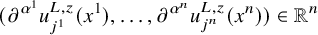 $$\begin{align*}({\partial}^{{\alpha}^1}u_{j^1}^{L,z}(x^1), \dots, {\partial}^{{\alpha}^n}u_{j^n}^{L,z}(x^n))\in{\mathbb{R}}^{n} \end{align*}$$
converge in distribution to the Gaussian vector
 $$ \begin{align} ({\partial}^{{\alpha}^1}u_{j^1}(x^1),\dots, {\partial}^{{\alpha}^n}u_{j^n}(x^n)) \end{align} $$
as $L\to \infty $
. This follows from the fact that their probability density functions are completely determined by the
$L\to \infty $
. This follows from the fact that their probability density functions are completely determined by the $n\times n$
variance matrix
$n\times n$
variance matrix
 $$\begin{align*}{\Sigma}^L:= \Big({\partial}_x^{{\alpha}^l}{\partial}_y^{{\alpha}^m}\kappa_{j^lj^m}^{L,z}(x,y)\big|_{(x,y)=(x^l,x^m)}\Big)_{1\leqslant l,m\leqslant n}\,, \end{align*}$$
which converges to ${\Sigma }:=({\partial }_x^{{\alpha }^l}{\partial }_y^{{\alpha }^m}\kappa _{j^lj^m}(x,y)|_{(x,y)=(x^l,x^m)})$
as
${\Sigma }:=({\partial }_x^{{\alpha }^l}{\partial }_y^{{\alpha }^m}\kappa _{j^lj^m}(x,y)|_{(x,y)=(x^l,x^m)})$
as $L\to \infty $
by Proposition 7.1. The latter, of course, is the covariance matrix of the Gaussian vector (7.5).
$L\to \infty $
by Proposition 7.1. The latter, of course, is the covariance matrix of the Gaussian vector (7.5).
It is well known that this convergence of arbitrary Gaussian vectors is not enough to conclude that $\mu ^{L,z}_R$
converges weakly to
$\mu ^{L,z}_R$
converges weakly to $\mu _{u,R}$
. However, notice that, for any integer
$\mu _{u,R}$
. However, notice that, for any integer $s\geqslant 0$
, the mean of the
$s\geqslant 0$
, the mean of the $H^s$
-norm of
$H^s$
-norm of $u^{L,z}$
is uniformly bounded:
$u^{L,z}$
is uniformly bounded:
 $$ \begin{align*} {\mathbb{E}}^{L,z}\|w\|_{H^s(B_R)}^2&=\sum_{|{\alpha}|\leqslant s}{\mathbb{E}}\int_{B_R} |D^{\alpha} u^{L,z}(x)|^2\, dx\\ &=\sum_{|{\alpha}|\leqslant s}\int_{B_R} \operatorname{\mathrm{tr}}\Big(D_x^{\alpha} D_y^{\alpha} \kappa^{L,z}(x,y)\big|_{y=x}\Big)\, dx\\ &\xrightarrow[L\to\infty]{\phantom{L}} \sum_{|{\alpha}|\leqslant s}\int_{B_R} \operatorname{\mathrm{tr}} \Big(D_x^{\alpha} D_y^{\alpha}\kappa(x,y)\big|_{y=x}\Big)\, dx<M_{s,R}\,. \end{align*} $$
To pass to the last line, we have used Proposition 7.1 once more. As the constant $M_{s,R}$
is independent of L, Sobolev’s inequality ensures that
$M_{s,R}$
is independent of L, Sobolev’s inequality ensures that
 $$\begin{align*}\sup_L{\mathbb{E}}^{L,z} \|w\|_{C^{k+1}(B_R)}^2\leqslant C\sup_L{\mathbb{E}}^{L,z} \|w\|^2_{H^{k+3}(B_R)}<M \end{align*}$$
for some constant M that only depends on R. For any $\varepsilon>0$
, this implies that for all admissible L large enough
$\varepsilon>0$
, this implies that for all admissible L large enough
 $$\begin{align*}\mu^{L,z}_R\big(\big\{ w\in C^k(B_R,{\mathbb{R}}^3): \|w\|_{C^{k+1}(B_R)}^2> M/\varepsilon\big\}\big)<\varepsilon\,. \end{align*}$$
As the set $\{ w\in C^k(B_R,{\mathbb {R}}^3): \|w\|_{C^{k+1}(B_R)}^2\leqslant M/\varepsilon \}$
is compact by the Arzelà–Ascoli theorem, we conclude that the sequence of probability measures
$\{ w\in C^k(B_R,{\mathbb {R}}^3): \|w\|_{C^{k+1}(B_R)}^2\leqslant M/\varepsilon \}$
is compact by the Arzelà–Ascoli theorem, we conclude that the sequence of probability measures $\mu ^{L,z}_R$
is tight. Therefore, a straightforward extension to jet spaces of the classical results about the convergence of probability measures on the space of continuous functions [Reference Billingsley7, Theorem 7.1], carried out in [Reference Wilson34], permits to conclude that
$\mu ^{L,z}_R$
is tight. Therefore, a straightforward extension to jet spaces of the classical results about the convergence of probability measures on the space of continuous functions [Reference Billingsley7, Theorem 7.1], carried out in [Reference Wilson34], permits to conclude that $\mu ^{L,z}_R$
indeed converges weakly to
$\mu ^{L,z}_R$
indeed converges weakly to $\mu _{u,R}$
as
$\mu _{u,R}$
as $L\to \infty $
. The lemma is then proven.
$L\to \infty $
. The lemma is then proven.
7.4 Proof of Theorem 1.6
We are now ready to prove our asymptotic estimates for high-frequency Beltrami fields on the torus. The basic idea is that, by the definition of the rescaling,
 $$\begin{align*}\mu^L\big(\big\{ w\in C^k({\mathbb{T}}^3,{\mathbb{R}}^3): N^{\mathrm{h}}_w>m\big\}\big)\geqslant \mu^{L,z}_R\big(\big\{ w\in C^k(B_R,{\mathbb{R}}^3): N^{\mathrm{h}}_w(r)>m\big\}\big) \end{align*}$$
provided that $r<R<L^{1/2}$
: this just means that the number of horseshoes that
$r<R<L^{1/2}$
: this just means that the number of horseshoes that $u^L$
has in the whole torus is certainly not less than those that are contained in a ball centered at any given point
$u^L$
has in the whole torus is certainly not less than those that are contained in a ball centered at any given point $z\in {\mathbb {T}}^3$
of radius
$z\in {\mathbb {T}}^3$
of radius $r/L^{1/2}<1$
. The same is clearly true as well when one counts invariant solid tori, periodic orbits or zeros instead.
$r/L^{1/2}<1$
. The same is clearly true as well when one counts invariant solid tori, periodic orbits or zeros instead.
For the ease of notation, let us denote by $\Phi _r(w)$
the quantity
$\Phi _r(w)$
the quantity $N^{\mathrm {h}}_w(r)$
,
$N^{\mathrm {h}}_w(r)$
, $N^{\mathrm {t}}_w(r;[{\mathcal T}],{\mathcal {J}},V_0)$
,
$N^{\mathrm {t}}_w(r;[{\mathcal T}],{\mathcal {J}},V_0)$
, $N^{\mathrm {o}}_w(r;[\gamma ],{\mathcal {I}})$
or
$N^{\mathrm {o}}_w(r;[\gamma ],{\mathcal {I}})$
or $N^{\mathrm {z}}_w(r)$
(that is, the number of nondegenerate zeros of w in
$N^{\mathrm {z}}_w(r)$
(that is, the number of nondegenerate zeros of w in $B_r$
), in each case. See Sections 4 and 5 for precise definitions. We recall that
$B_r$
), in each case. See Sections 4 and 5 for precise definitions. We recall that $N^{\mathrm {z}}_w(r)={\mathcal {N}}(r;{\mathcal {X}}_w)$
with probability
$N^{\mathrm {z}}_w(r)={\mathcal {N}}(r;{\mathcal {X}}_w)$
with probability $1$
, cf. Section 6.3. Theorems 6.2 (for periodic orbits, invariant tori and horseshoes) and 1.5 (for zeros) ensure that, given any
$1$
, cf. Section 6.3. Theorems 6.2 (for periodic orbits, invariant tori and horseshoes) and 1.5 (for zeros) ensure that, given any $m_1>0$
, any
$m_1>0$
, any $\delta _1>0$
, any closed curve
$\delta _1>0$
, any closed curve $\gamma $
and any embedded torus
$\gamma $
and any embedded torus ${\mathcal T}$
, one can find some parameters
${\mathcal T}$
, one can find some parameters ${\mathcal {I}}$
,
${\mathcal {I}}$
, ${\mathcal {J}}$
,
${\mathcal {J}}$
, $V_0$
and
$V_0$
and $r>0$
such that
$r>0$
such that
 $$\begin{align*}\mu_u\big(\big \{w\in C^k({\mathbb{R}}^3,{\mathbb{R}}^3): \Phi_r(w)>m_1 \big\}\big)>1-\delta_1\,. \end{align*}$$
Of course, here we are simply using that the volume $|B_r|$
, which appears in the statements of Theorems 6.2 and 1.5 but not here, can be made arbitrarily large by taking a large r.
$|B_r|$
, which appears in the statements of Theorems 6.2 and 1.5 but not here, can be made arbitrarily large by taking a large r.
Let us now fix a constant $R>r$
and a point
$R>r$
and a point $z\in {\mathbb {T}}^3$
. We showed in Propositions 4.1, 4.6, 5.1 and 6.4 that the functionals that we are now denoting by
$z\in {\mathbb {T}}^3$
. We showed in Propositions 4.1, 4.6, 5.1 and 6.4 that the functionals that we are now denoting by $\Phi _r$
are lower semicontinuous on the space
$\Phi _r$
are lower semicontinuous on the space $C^k({\mathbb {R}}^3,{\mathbb {R}}^3)$
of divergence-free fields for
$C^k({\mathbb {R}}^3,{\mathbb {R}}^3)$
of divergence-free fields for $k\geqslant 4$
. This implies that the set
$k\geqslant 4$
. This implies that the set
 $$\begin{align*}\Omega_{r,R,m_1}:=\{w\in C^k(B_R,{\mathbb{R}}^3): \Phi_r(w)>m_1\} \end{align*}$$
is open in $C^k(B_R,{\mathbb {R}}^3)$
. Lemma 7.2 ensures that the measure
$C^k(B_R,{\mathbb {R}}^3)$
. Lemma 7.2 ensures that the measure $\mu ^{L,z}_R$
converges weakly to
$\mu ^{L,z}_R$
converges weakly to $\mu _{u,R}$
as
$\mu _{u,R}$
as $L\to \infty $
through the admissible integers. As the set
$L\to \infty $
through the admissible integers. As the set $\Omega _{r,R,m_1}$
is open, this is well-known to imply (see, e.g., [Reference Billingsley7, Theorem 2.1.iv]) that
$\Omega _{r,R,m_1}$
is open, this is well-known to imply (see, e.g., [Reference Billingsley7, Theorem 2.1.iv]) that
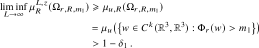 $$ \begin{align*} \liminf_{L\to\infty}\mu^{L,z}_R(\Omega_{r,R,m_1})&\geqslant \mu_{u,R}(\Omega_{r,R,m_1})\\ &=\mu_u\big( \big\{w\in C^k({\mathbb{R}}^3,{\mathbb{R}}^3): \Phi_r(w)>m_1 \big\}\big)\\ &>1-\delta_1\,. \end{align*} $$
We observe that $\delta _1>0$
can be taken arbitrarily small if r is large enough (and
$\delta _1>0$
can be taken arbitrarily small if r is large enough (and $r/L^{1/2}<R/L^{1/2}<1$
). Now, for any
$r/L^{1/2}<R/L^{1/2}<1$
). Now, for any $A\geqslant 1$
and L large enough, we can take A pairwise disjoint balls in
$A\geqslant 1$
and L large enough, we can take A pairwise disjoint balls in ${\mathbb {T}}^3$
of radius
${\mathbb {T}}^3$
of radius $r/L^{1/2}<A^{-1/3}$
centered at points
$r/L^{1/2}<A^{-1/3}$
centered at points $\{z^a\}_{a=1}^A\subset {\mathbb {T}}^3$
. Setting
$\{z^a\}_{a=1}^A\subset {\mathbb {T}}^3$
. Setting $m:=Am_1$
, the previous analysis, which is independent of the point z, readily implies that
$m:=Am_1$
, the previous analysis, which is independent of the point z, readily implies that
 $$\begin{align*}\mu^L\big(\big\{ w\in C^k({\mathbb{T}}^3,{\mathbb{R}}^3): N^{\mathrm{X},\mathrm{e}}_w>m\big\}\big)\geqslant 1-2A\delta_1>1-\delta\,, \end{align*}$$
where the superscript X stands for $\mathrm {h,t,o}$
or
$\mathrm {h,t,o}$
or $\mathrm {z}$
, thus proving the part of the statement concerning the number of approximately equidistributed horseshoes, invariant tori isotopic to
$\mathrm {z}$
, thus proving the part of the statement concerning the number of approximately equidistributed horseshoes, invariant tori isotopic to ${\mathcal T}$
, periodic orbits isotopic to
${\mathcal T}$
, periodic orbits isotopic to $\gamma $
or zeros. In fact, concerning invariant tori, we observe that obviously
$\gamma $
or zeros. In fact, concerning invariant tori, we observe that obviously $N^{\mathrm {t}}_w(r;[{\mathcal T}])=\infty $
if
$N^{\mathrm {t}}_w(r;[{\mathcal T}])=\infty $
if $N^{\mathrm {t}}_w(r;[{\mathcal T}],{\mathcal {J}},V_0)\geqslant 1$
. Since the previous estimate ensures that
$N^{\mathrm {t}}_w(r;[{\mathcal T}],{\mathcal {J}},V_0)\geqslant 1$
. Since the previous estimate ensures that $N^{\mathrm {t}}_w(r;[{\mathcal T}],{\mathcal {J}},V_0)>m_1$
with probability
$N^{\mathrm {t}}_w(r;[{\mathcal T}],{\mathcal {J}},V_0)>m_1$
with probability $1$
as
$1$
as $L\to \infty $
, we infer that the probability of having an infinite number of (Diophantine) invariant tori isotopic to
$L\to \infty $
, we infer that the probability of having an infinite number of (Diophantine) invariant tori isotopic to ${\mathcal T}$
also tends to 1 as
${\mathcal T}$
also tends to 1 as $L\to \infty $
through the admissible integers. However, this does not provide any information about the expected volume of the invariant tori.
$L\to \infty $
through the admissible integers. However, this does not provide any information about the expected volume of the invariant tori.
The result about the topological entropy follows from the following observation. If we denote by $\phi ^L_t$
the time-t flow of the Beltrami field
$\phi ^L_t$
the time-t flow of the Beltrami field $u^L(z+\cdot )$
, and by
$u^L(z+\cdot )$
, and by $\phi _t$
the flow of the rescaled field
$\phi _t$
the flow of the rescaled field $u^{L,z}$
, it is evident that
$u^{L,z}$
, it is evident that
 $$\begin{align*}\phi^L_t=\frac{1}{L^{1/2}}\phi_{L^{1/2}t}\,. \end{align*}$$
Then, the topological entropy ${h_{\mathrm {top}}}(u^L)$
, which is defined as the entropy of its time-
${h_{\mathrm {top}}}(u^L)$
, which is defined as the entropy of its time- $1$
flow, satisfies
$1$
flow, satisfies
 $$ \begin{align} {h_{\mathrm{top}}}(u^L)&={h_{\mathrm{top}}}(\phi^L_1)={h_{\mathrm{top}}} \Big(\frac{1}{L^{1/2}}\phi_{L^{1/2}}\Big)={h_{\mathrm{top}}}(\phi_{L^{1/2}})=L^{1/2}{h_{\mathrm{top}}}(\phi_1) \end{align} $$
 $$ \begin{align} &\hspace{-36pt}=L^{1/2}{h_{\mathrm{top}}}(u^{L,z})\,. \end{align} $$
In the third equality, we have used that the topological entropy does not depend on the space scale (or equivalently, on the metric), and in the fourth equality we have used Abramov’s well-known formula (see, e.g., [Reference Gelfert and Motter19]). Since the rescaled field has a horseshoe in a ball of radius r with probability $1$
as
$1$
as $L\to \infty $
, and a horseshoe has positive topological entropy, say larger than some constant
$L\to \infty $
, and a horseshoe has positive topological entropy, say larger than some constant ${\nu ^{\mathrm {h}}}_*$
(see Proposition 5.1), equation (7.6) implies that the topological entropy of
${\nu ^{\mathrm {h}}}_*$
(see Proposition 5.1), equation (7.6) implies that the topological entropy of $u^L$
is at least
$u^L$
is at least ${\nu ^{\mathrm {h}}}_* L^{1/2}$
.
${\nu ^{\mathrm {h}}}_* L^{1/2}$
.
Finally, we prove the statement about the expected values. As above, we use the functional $\Phi _r(w)$
to denote the number of different objects (horseshoes, solid tori or periodic orbits). The case of zeros will be considered later. Note that, since
$\Phi _r(w)$
to denote the number of different objects (horseshoes, solid tori or periodic orbits). The case of zeros will be considered later. Note that, since $\Phi _r$
is lower semicontinuous, and
$\Phi _r$
is lower semicontinuous, and $\mu ^{L,z}$
converges weakly to
$\mu ^{L,z}$
converges weakly to $\mu _u$
as
$\mu _u$
as $L\to \infty $
by Lemma 7.2, it is standard that [Reference Billingsley7, Exercise 2.6]
$L\to \infty $
by Lemma 7.2, it is standard that [Reference Billingsley7, Exercise 2.6]
 $$\begin{align*}\liminf_{L\to\infty}{\mathbb{E}}^{L,z}\frac{\Phi_r}{|B_r|}\geqslant {\mathbb{E}} \frac{\Phi_r}{|B_r|}\geqslant \eta>0\,, \end{align*}$$
where we have picked some fixed, large enough r. Here, we have used the asymptotics in ${\mathbb {R}}^3$
, given by Theorem 6.2, to infer that the last expectation is positive if r is large. Notice that the constant
${\mathbb {R}}^3$
, given by Theorem 6.2, to infer that the last expectation is positive if r is large. Notice that the constant $\eta $
depends on
$\eta $
depends on $[\gamma ],[{\mathcal T}],{\mathcal {I}}$
or
$[\gamma ],[{\mathcal T}],{\mathcal {I}}$
or ${\mathcal {J}}$
depending on the functional that we are considering, but we shall not write this dependence explicitly. Furthermore, as the distribution of the measure
${\mathcal {J}}$
depending on the functional that we are considering, but we shall not write this dependence explicitly. Furthermore, as the distribution of the measure $\mu ^{L,z}_R$
is in fact independent of z by Proposition 7.1, this ensures that there is some
$\mu ^{L,z}_R$
is in fact independent of z by Proposition 7.1, this ensures that there is some $L_0$
independent of z such that
$L_0$
independent of z such that
 $$\begin{align*}{\mathbb{E}}^{L,z}\frac{\Phi_r}{|B_r|}> \frac\eta2 \end{align*}$$
for all admissible $L>L_0$
and all
$L>L_0$
and all $z\in {\mathbb {T}}^3$
.
$z\in {\mathbb {T}}^3$
.
Now, given any admissible $L>L_0$
, it is standard that we can cover the torus
$L>L_0$
, it is standard that we can cover the torus ${\mathbb {T}}^3$
by balls
${\mathbb {T}}^3$
by balls $\{ B_{r_L}(z^a): 1\leqslant a\leqslant A_L\}$
of radius
$\{ B_{r_L}(z^a): 1\leqslant a\leqslant A_L\}$
of radius $r_L:=2r/L^{1/2}$
centered at
$r_L:=2r/L^{1/2}$
centered at $z^a\in {\mathbb {T}}^3$
such that the smaller balls
$z^a\in {\mathbb {T}}^3$
such that the smaller balls $B_{r_L/2}(z^a)$
are pairwise disjoint. This implies that
$B_{r_L/2}(z^a)$
are pairwise disjoint. This implies that $A_L\geqslant c L^{\frac 32}$
for some dimensional constant c. The expected value of, say, the number of horseshoes of
$A_L\geqslant c L^{\frac 32}$
for some dimensional constant c. The expected value of, say, the number of horseshoes of $u^L$
in
$u^L$
in ${\mathbb {T}}^3$
can then be controlled as follows, for any admissible
${\mathbb {T}}^3$
can then be controlled as follows, for any admissible $L>L_0$
:
$L>L_0$
:
 $$ \begin{align*} \frac{{\mathbb{E}}^L N^{\mathrm h}}{L^{3/2}} &\geqslant \sum_{a=1}^{A_L} \frac{|B_r|}{L^{3/2}} \, {\mathbb{E}}^{L,z^a} \frac{\Phi_r }{|B_r|}\\ &\geqslant \frac{c|B_r|\eta}2>\nu_* \end{align*} $$
for some positive constant $\nu _*$
independent of L. An analogous estimate holds for the expected value
$\nu _*$
independent of L. An analogous estimate holds for the expected value ${\mathbb {E}}^L N^{\mathrm o}([\gamma ])$
.
${\mathbb {E}}^L N^{\mathrm o}([\gamma ])$
.
To estimate the volume of ergodic invariant tori isotopic to ${\mathcal T}$
, we can proceed as follows. For any admissible
${\mathcal T}$
, we can proceed as follows. For any admissible $L>L_0$
, we have:
$L>L_0$
, we have:
 $$ \begin{align*} {\mathbb{E}}^L V^{\mathrm{t}}([{\mathcal T}]) &\geqslant \sum_{a=1}^{A_L} |B_{r_L/2}| \, {\mathbb{E}}^{L,z^a} \frac{V^{\mathrm{t}}(r;[{\mathcal T}],{\mathcal{J}}) }{|B_r|}\\ &\geqslant \sum_{a=1}^{A_L} |B_{r_L/2}| \, V_0\, {\mathbb{E}}^{L,z^a} \frac{\Phi_r }{|B_r|}\\ &\geqslant \frac{V_0\eta}2\sum_{a=1}^{A_L} |B_{r_L/2}|>\nu^{\mathrm{t}}_*([{\mathcal T}]) \end{align*} $$
for some positive constant $\nu ^{\mathrm {t}}_*([{\mathcal T}])$
independent of L. Here, we have used that the balls
$\nu ^{\mathrm {t}}_*([{\mathcal T}])$
independent of L. Here, we have used that the balls $B_{r_L/2} (z^a)$
are pairwise disjoint and the sum of their volumes is, by construction, larger than
$B_{r_L/2} (z^a)$
are pairwise disjoint and the sum of their volumes is, by construction, larger than $|{\mathbb {T}}^3|/8$
.
$|{\mathbb {T}}^3|/8$
.
Lastly, in the following lemma we consider the case of zeros:
Lemma 7.3. $\displaystyle {\mathbb {E}}^L(L^{-\frac 32}{N^{\mathrm {z}}_{u^L}})\to (2\pi )^3{\nu ^{\mathrm {z}}}$
as
$\displaystyle {\mathbb {E}}^L(L^{-\frac 32}{N^{\mathrm {z}}_{u^L}})\to (2\pi )^3{\nu ^{\mathrm {z}}}$
as $L\to \infty $
through admissible values.
$L\to \infty $
through admissible values.
Proof. Let us use the notation
 $$\begin{align*}Q_R:=(-R\pi,R\pi)\times (-R\pi,R\pi)\times(-R\pi,R\pi) \end{align*}$$
for the open cube of side $2\pi R$
in
$2\pi R$
in ${\mathbb {R}}^3$
and call
${\mathbb {R}}^3$
and call $N_{u^L}^{\mathrm {z},*}$
the number of zeros of
$N_{u^L}^{\mathrm {z},*}$
the number of zeros of $u^L$
(or rather of its periodic lift to
$u^L$
(or rather of its periodic lift to ${\mathbb {R}}^3$
) that are contained in
${\mathbb {R}}^3$
) that are contained in $Q_1$
. By Bulinskaya’s lemma [Reference Azais and Wschebor4, Proposition 6.11], with probability 1 the zero set of
$Q_1$
. By Bulinskaya’s lemma [Reference Azais and Wschebor4, Proposition 6.11], with probability 1 the zero set of $u^L$
is nondegenerate (and hence a finite set of points) and the lift of
$u^L$
is nondegenerate (and hence a finite set of points) and the lift of $u^L$
does not have any zeros on the boundary
$u^L$
does not have any zeros on the boundary ${\partial } Q_1$
. Therefore, for any positive integer R,
${\partial } Q_1$
. Therefore, for any positive integer R,
 $$\begin{align*}{N^{\mathrm{z}}_{u^L}}= N_{u^L}^{\mathrm{z},*} \end{align*}$$
almost surely. In particular, both quantities have the same expectation.
Let us now take some small positive real r and denote by ${N^{\mathrm {z}}_{u^L}}(y,r)$
the number of zeros of
${N^{\mathrm {z}}_{u^L}}(y,r)$
the number of zeros of $u^L$
(or rather of its lift to
$u^L$
(or rather of its lift to ${\mathbb {R}}^3$
) that are contained in the ball
${\mathbb {R}}^3$
) that are contained in the ball $B_r(y)$
. The argument we used to prove the estimate for
$B_r(y)$
. The argument we used to prove the estimate for ${\mathcal {N}}(R;{\mathcal {X}})$
in Lemma 6.1 (starting now from the number of zeros in
${\mathcal {N}}(R;{\mathcal {X}})$
in Lemma 6.1 (starting now from the number of zeros in $Q_1$
instead of in
$Q_1$
instead of in $B_R$
) shows that
$B_R$
) shows that
 $$\begin{align*}\int_{Q_{1-r}}\frac{{N^{\mathrm{z}}_{u^L}}(z,r)}{|B_r|}\, dz\leqslant N_{u^L}^{\mathrm{z},*}\leqslant \int_{Q_{1+r}}\frac{{N^{\mathrm{z}}_{u^L}}(z,r)}{|B_r|}\, dz\,. \end{align*}$$
Note now that
 $$\begin{align*}\int_{Q_{1\pm r}}\frac{{N^{\mathrm{z}}_{u^L}}(z,r)}{|B_r|}\, dz=L^{\frac32}\int_{Q_{1\pm r}}\frac{{N^{\mathrm{z}}_{u^{L,z}}}(rL^{1/2})}{|B_{rL^{1/2}}|}\, dz\,. \end{align*}$$
The expected value of this quantity is
 $$ \begin{align*} {\mathbb{E}}^L \int_{Q_{1\pm r}}\frac{{N^{\mathrm{z}}_{u^{L,z}}}(rL^{1/2})}{|B_{rL^{1/2}}|}\, dz&=\int_{Q_{1\pm r}}\frac{{\mathbb{E}}^{L,z}{N^{\mathrm{z}}_{u^{L,z}}}(rL^{1/2})}{|B_{rL^{1/2}}|}\, dz\\ &=|Q_{1\pm r}|\frac{{\mathbb{E}}^{L,z}{N^{\mathrm{z}}_{u^{L,z}}}(rL^{1/2})}{|B_{rL^{1/2}}|}\,. \end{align*} $$
To pass to the second line, we have used that the expected value inside the integral is independent of the point z by Proposition 7.1; in particular, this value is independent of the point z one considers.
We can now argue just as in the case of ${\mathbb {R}}^3$
, discussed in detail in Subsection 6.3, so we will just sketch the arguments and refer to that subsection for the notation. The Kac–Rice formula ensures
${\mathbb {R}}^3$
, discussed in detail in Subsection 6.3, so we will just sketch the arguments and refer to that subsection for the notation. The Kac–Rice formula ensures
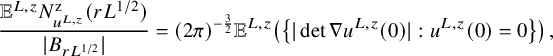 $$ \begin{align*} \frac{{\mathbb{E}}^{L,z}{N^{\mathrm{z}}_{u^{L,z}}}(rL^{1/2})}{|B_{rL^{1/2}}|}&= (2\pi)^{-\frac32}{\mathbb{E}}^{L,z}\big(\big\{ | \det \nabla u^{L,z}(0)|: u^{L,z}(0)=0\big\}\big)\,, \end{align*} $$
and this conditional expectation can be transformed into an unconditional one just as in the proof of Lemma 6.5:
 $$ \begin{align*} \frac{{\mathbb{E}}^{L,z}{N^{\mathrm{z}}_{u^{L,z}}}(rL^{1/2})}{|B_{rL^{1/2}}|}&=(2\pi)^{-3/2}{\mathbb{E}}^{L,z}(|\det\zeta^{L,z}|)\\ &= \frac{(2\pi)^{-3/2}}{(2\pi)^{5/2}(\det {\Sigma}^{\prime L,z})^{1/2}}\int_{{\mathbb{R}}^5}Q^{L,z}(\zeta')\, &=:\nu^{\mathrm{z},L,z}\,. \end{align*} $$
The fact that the covariance matrix of $u^{L,z}$
converges to that of u as
$u^{L,z}$
converges to that of u as $L\to \infty $
by Proposition 7.1 implies that
$L\to \infty $
by Proposition 7.1 implies that
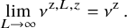 $$\begin{align*}\lim_{L\to\infty}\nu^{\mathrm{z},L,z}={\nu^{\mathrm{z}}}\,. \end{align*}$$
Hence, writing the aforementioned sandwich estimate as
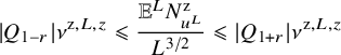 $$\begin{align*}|Q_{1-r}|\nu^{\mathrm{z},L,z}\leqslant \frac{{\mathbb{E}}^L{N^{\mathrm{z}}_{u^L}}}{L^{3/2}}\leqslant |Q_{1+r}|\nu^{\mathrm{z},L,z} \end{align*}$$
and letting $L\to \infty $
and then
$L\to \infty $
and then $r\to 0$
, we infer that
$r\to 0$
, we infer that
 $$\begin{align*}\lim_{L\to\infty}\frac{{\mathbb{E}}^L{N^{\mathrm{z}}_{u^L}}}{L^{3/2}}= |Q_1|{\nu^{\mathrm{z}}}=(2\pi)^3{\nu^{\mathrm{z}}}\,. \end{align*}$$
The lemma follows.
Theorem 1.6 is then proven.
Appendix A. Fourier-theoretic characterization of Beltrami fields
For the benefit of the reader, in this appendix we describe what polynomially bounded Beltrami fields look like in Fourier space. As Beltrami fields are a particular class of vector-valued monochromatic waves, it is convenient to start the discussion by considering polynomially bounded solutions to the Helmholtz equation
 $$\begin{align*}{\Delta} F + F=0\,. \end{align*}$$
As before, we consider the case of monochromatic waves on ${\mathbb {R}}^3$
, but the analysis applies essentially verbatim to any other dimension. The Fourier transform of this equation shows that
${\mathbb {R}}^3$
, but the analysis applies essentially verbatim to any other dimension. The Fourier transform of this equation shows that
 $$\begin{align*}(1-|\xi|^2){{\widehat{F}}}(\xi)=0\,, \end{align*}$$
so the support of ${{\widehat {F}}}$
must be contained in the unit sphere,
${{\widehat {F}}}$
must be contained in the unit sphere, ${\mathbb {S}}$
. In spherical coordinates
${\mathbb {S}}$
. In spherical coordinates $\rho :=|\xi |\in {\mathbb {R}}^+$
and
$\rho :=|\xi |\in {\mathbb {R}}^+$
and $\omega :=\xi /|\xi |\in {\mathbb {S}}$
, it is standard that this is equivalent to saying that
$\omega :=\xi /|\xi |\in {\mathbb {S}}$
, it is standard that this is equivalent to saying that ${{\widehat {F}}}$
is a finite sum of the form
${{\widehat {F}}}$
is a finite sum of the form
 $$\begin{align*}{{\widehat{F}}}= \sum_{n=1}^N F_n(\omega)\, \delta^{(n)}(\rho-1)\,. \end{align*}$$
Here, $\delta ^{(n)}$
is the
$\delta ^{(n)}$
is the $n^{\mathrm {th}}$
derivative of the Dirac measure and
$n^{\mathrm {th}}$
derivative of the Dirac measure and $F_n$
is a distribution on the sphere, so
$F_n$
is a distribution on the sphere, so $F_n\in H^{s_n}({\mathbb {S}})$
for some
$F_n\in H^{s_n}({\mathbb {S}})$
for some $s_n\in {\mathbb {R}}$
(because any compactly supported distribution is in a Sobolev space, possibly of negative order). Note that F is real-valued if and only if the functions
$s_n\in {\mathbb {R}}$
(because any compactly supported distribution is in a Sobolev space, possibly of negative order). Note that F is real-valued if and only if the functions $F_n$
are Hermitian. Of course, there are also monochromatic waves that are not polynomially bounded, such as
$F_n$
are Hermitian. Of course, there are also monochromatic waves that are not polynomially bounded, such as $F:= e^{x_1}\cos (\sqrt 2 \, x_2)$
.
$F:= e^{x_1}\cos (\sqrt 2 \, x_2)$
.
A classical result due to Herglotz [Reference Hörmander26, Theorem 7.1.28] ensures that if F is a monochromatic wave with the sharp fall-off at infinity, that is, such that
 $$\begin{align*}\limsup_{R\to\infty}\frac1R \int_{B_R}F^2\, dx<\infty\,, \end{align*}$$
then there is a Hermitian vector-valued function $f\in L^2({\mathbb {S}})$
such that
$f\in L^2({\mathbb {S}})$
such that ${{\widehat {F}}} = f\, \delta (\rho -1)$
. Furthermore, the value of the above limit is in the interval
${{\widehat {F}}} = f\, \delta (\rho -1)$
. Furthermore, the value of the above limit is in the interval $[C_1\|F\|^2_{L^2({\mathbb {S}})},C_2\|F\|^2_{L^2({\mathbb {S}})}]$
for some constants
$[C_1\|F\|^2_{L^2({\mathbb {S}})},C_2\|F\|^2_{L^2({\mathbb {S}})}]$
for some constants $C_1,C_2$
. This bound means that, on an average sense,
$C_1,C_2$
. This bound means that, on an average sense, $|F(x)|$
decays as
$|F(x)|$
decays as $C/|x|$
. The prime example of this behavior is given by
$C/|x|$
. The prime example of this behavior is given by $f=1$
, which corresponds to
$f=1$
, which corresponds to $F(x)=c |x|^{-1/2} J_{1/2}(|x|)$
.
$F(x)=c |x|^{-1/2} J_{1/2}(|x|)$
.
The expression (1.3) corresponds to the case $N=0$
above, since the function
$N=0$
above, since the function $F_0$
with
$F_0$
with ${{\widehat {F}}}_0=f(\omega )\, \delta (\rho -1)$
is precisely
${{\widehat {F}}}_0=f(\omega )\, \delta (\rho -1)$
is precisely
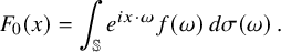 $$\begin{align*}F_0(x)=\int_{\mathbb{S}} e^{ix\cdot\omega} f(\omega)\, d{\sigma}(\omega)\,. \end{align*}$$
Also, if $f\in H^{-k}({\mathbb {S}})$
with
$f\in H^{-k}({\mathbb {S}})$
with $k\geqslant 0$
but not necessarily in
$k\geqslant 0$
but not necessarily in $L^2({\mathbb {S}})$
, the function
$L^2({\mathbb {S}})$
, the function $F_0$
is bounded as [Reference Enciso, Peralta-Salas and Romaniega15, Appendix A]
$F_0$
is bounded as [Reference Enciso, Peralta-Salas and Romaniega15, Appendix A]
 $$ \begin{align} \sup_{R>0} \frac1R\int_{B_R}\frac{F_0(x)^2}{1+|x|^{2k}}\, dx\leqslant C\|f\|^2_{H^{-k}({\mathbb{S}})}\,. \end{align} $$
Hence, in this case, $F_0$
is bounded, on an average sense, by
$F_0$
is bounded, on an average sense, by $C|x|^{k-1}$
. Therefore, if
$C|x|^{k-1}$
. Therefore, if $f\in H^{-1}({\mathbb {S}})$
,
$f\in H^{-1}({\mathbb {S}})$
, $F_0$
is uniformly bounded in average sense.
$F_0$
is uniformly bounded in average sense.
If f is a Gaussian random field, as considered in the Nazarov–Sodin theory (see equation (1.3a)), we showed in Proposition 3.2 that f is almost surely in $H^{-1-\delta }({\mathbb {S}})$
for all
$H^{-1-\delta }({\mathbb {S}})$
for all $\delta>0$
and not in
$\delta>0$
and not in $L^2({\mathbb {S}})$
. This behavior morally corresponds to functions that are bounded on a average sense but do not decay at infinity, as illustrated by the function
$L^2({\mathbb {S}})$
. This behavior morally corresponds to functions that are bounded on a average sense but do not decay at infinity, as illustrated by the function $F_0:=\cos x_1$
generated by
$F_0:=\cos x_1$
generated by $f:= \frac 12[\delta _{\xi _+}(\xi )+ \delta _{\xi _-}(\xi )]$
. This is the kind of behavior one needs to describe the expected local behavior of a high-energy eigenfunction on a compact manifold as one zooms in at a given point.
$f:= \frac 12[\delta _{\xi _+}(\xi )+ \delta _{\xi _-}(\xi )]$
. This is the kind of behavior one needs to describe the expected local behavior of a high-energy eigenfunction on a compact manifold as one zooms in at a given point.
The monochromatic wave defined as ${{\widehat {F}}}_n:= f(\omega )\,\delta ^{(n)}(\rho -1)$
reads, in physical space, as
${{\widehat {F}}}_n:= f(\omega )\,\delta ^{(n)}(\rho -1)$
reads, in physical space, as
 $$ \begin{align*} F_n(x)=\int_{{\mathbb{S}}}\int_0^{\infty} e^{i\rho x\cdot \omega} f(\omega)\,\rho^2\, \delta^{(n)}(\rho-1)\, d\rho\, d{\sigma}(\omega) =(-1)^n \int_{\mathbb{S}} f(\omega)\, {\partial}_{\rho}^n|_{\rho=1}(\rho^2 e^{i\rho x\cdot \omega})\, d{\sigma}(\omega)\,. \end{align*} $$
Note that the $n^{\mathrm {th}}$
derivative term involves an
$n^{\mathrm {th}}$
derivative term involves an $n^{\mathrm {th}}$
power of x. Therefore, using the bound (A.1), one easily finds that
$n^{\mathrm {th}}$
power of x. Therefore, using the bound (A.1), one easily finds that $F_n$
is bounded on average as
$F_n$
is bounded on average as $C|x|^{n+k-1}$
if
$C|x|^{n+k-1}$
if $f\in H^{-k}({\mathbb {S}})$
; explicit examples with this growth can be easily constructed by taking f to be either a constant for
$f\in H^{-k}({\mathbb {S}})$
; explicit examples with this growth can be easily constructed by taking f to be either a constant for $k=0$
or the
$k=0$
or the $(k-1)^{\mathrm {th}}$
derivative of the Dirac measure for
$(k-1)^{\mathrm {th}}$
derivative of the Dirac measure for $k\geqslant 1$
. Consequently, picking f as in equation (1.3a), the bound (A.1) morally leads to thinking of
$k\geqslant 1$
. Consequently, picking f as in equation (1.3a), the bound (A.1) morally leads to thinking of $F_n$
as a function that grows as
$F_n$
as a function that grows as $|x|^n$
at infinity, which cannot be the localized behavior of an eigenfunction. This is the rationale for defining a random monochromatic wave as in equations (1.3a) and (1.3b). In this direction, let us recall that the relation between random monochromatic waves and zoomed-in high-energy eigenfunctions on various compact manifolds is an influential long-standing conjecture of Berry [Reference Berry6]. A precise form of this relation has been recently established in the case of the round sphere and of the flat torus [Reference Nazarov and Sodin29, Reference Nazarov and Sodin30, Reference Rozenshein31], which heuristically shows that equations (1.3a) and (1.3b) is indeed the proper definition of random monochromatic waves for this purpose.
$|x|^n$
at infinity, which cannot be the localized behavior of an eigenfunction. This is the rationale for defining a random monochromatic wave as in equations (1.3a) and (1.3b). In this direction, let us recall that the relation between random monochromatic waves and zoomed-in high-energy eigenfunctions on various compact manifolds is an influential long-standing conjecture of Berry [Reference Berry6]. A precise form of this relation has been recently established in the case of the round sphere and of the flat torus [Reference Nazarov and Sodin29, Reference Nazarov and Sodin30, Reference Rozenshein31], which heuristically shows that equations (1.3a) and (1.3b) is indeed the proper definition of random monochromatic waves for this purpose.
The reasoning leading to the definition of a random Beltrami field as equaiton (1.3) is completely analogous and the fact that one can relate Gaussian random Beltrami fields on ${\mathbb {R}}^3$
to high-frequency Beltrami fields on the torus just as in the case of the Nazarov–Sodin theory heuristically ensures that this is indeed the appropriate definition. For completeness, let us record that, just as in the case of monochromatic random waves, the Fourier transform of a polynomially bounded Beltrami field u is a finite sum of the form
${\mathbb {R}}^3$
to high-frequency Beltrami fields on the torus just as in the case of the Nazarov–Sodin theory heuristically ensures that this is indeed the appropriate definition. For completeness, let us record that, just as in the case of monochromatic random waves, the Fourier transform of a polynomially bounded Beltrami field u is a finite sum of the form
 $$\begin{align*}{\widehat{u}} = \sum_{n=1}^N f_n(\omega)\, \delta^{(n)}(\rho-1)\,, \end{align*}$$
where now $f_n$
is a Hermitian
$f_n$
is a Hermitian ${\mathbb {C}}^3$
-valued distribution on
${\mathbb {C}}^3$
-valued distribution on ${\mathbb {S}}$
. For u to be a Beltrami field, there is an additional constraint on
${\mathbb {S}}$
. For u to be a Beltrami field, there is an additional constraint on $f_n$
coming from the fact that not every distribution supported on
$f_n$
coming from the fact that not every distribution supported on ${\mathbb {S}}$
satisfies the equation
${\mathbb {S}}$
satisfies the equation $i\xi \times {\widehat {u}}(\xi )= {\widehat {u}}(\xi )$
. A straightforward computation shows that this constraint amounts to imposing that
$i\xi \times {\widehat {u}}(\xi )= {\widehat {u}}(\xi )$
. A straightforward computation shows that this constraint amounts to imposing that
 $$\begin{align*}\sum_{n=j}^N \binom nj {\alpha}_{n-j,2} f_n(\omega)= i\omega\times \sum_{n=j}^N \binom nj {\alpha}_{n-j,3} f_n(\omega) \end{align*}$$
on ${\mathbb {S}}$
for all
${\mathbb {S}}$
for all $0\leqslant j\leqslant N$
. Here,
$0\leqslant j\leqslant N$
. Here, ${\alpha }_{k,l}:= \prod _{m=0}^{k-1} (l-m)$
with the convention that
${\alpha }_{k,l}:= \prod _{m=0}^{k-1} (l-m)$
with the convention that ${\alpha }_{0,l}:=1$
. To see this, it suffices to note that the action of
${\alpha }_{0,l}:=1$
. To see this, it suffices to note that the action of ${\widehat {u}}$
and
${\widehat {u}}$
and $i\xi \times {\widehat {u}}$
on a vector field
$i\xi \times {\widehat {u}}$
on a vector field $w\in C^{\infty }_c({\mathbb {R}}^3,{\mathbb {R}}^3)$
is
$w\in C^{\infty }_c({\mathbb {R}}^3,{\mathbb {R}}^3)$
is
 $$ \begin{align*} \langle {\widehat{u}},w \rangle &= \sum_{n=0}^N (-1)^n\int_{\mathbb{S}} f_n(\omega)\cdot {\partial}_{\rho}^n|_{\rho=1} \left[\rho^2 w(\rho\omega)\right]\, d{\sigma}(\omega)\,,\\ \langle i\xi\times {\widehat{u}},w \rangle &= \sum_{n=0}^N (-1)^n\int_{\mathbb{S}} i\omega\times f_n(\omega)\cdot {\partial}_{\rho}^n|_{\rho=1} \left[\rho^3 w(\rho\omega)\right]\, d{\sigma}(\omega)\,, \end{align*} $$
expand the $n^{\mathrm {th}}$
derivative using the binomial formula and note that
$n^{\mathrm {th}}$
derivative using the binomial formula and note that ${\alpha }_{k,l}$
is the
${\alpha }_{k,l}$
is the $k^{\mathrm {th}}$
derivative of
$k^{\mathrm {th}}$
derivative of $\rho ^l$
at
$\rho ^l$
at $\rho =1$
.
$\rho =1$
.
Acknowledgements
The authors are deeply indebted to Alejandro Luque for the numerical computation of the Melnikov constants in Section 5.
Funding statement
A.E. is supported by the ERC Consolidator Grant 862342. The authors are also supported by the grant MTM PID2019-106715GB-C21 (D.P.-S. and A.R.) from Agencia Estatal de Investigación (AEI). This work is supported in part by the ICMAT–Severo Ochoa grant CEX2019-000904-S.
Competing interests
The authors have no competing interest to declare.
Data availability statement
Not applicable.
Ethical standards
The research meets all ethical guidelines, including adherence to the legal requirements of the study country.
Author contributions
A.E., D.P.-S. and A.R. designed the study, wrote the first draft and approved the final version of the manuscript.

 Open access