


1. Introduction
Land degradation in sub-Saharan Africa remains a substantial problem in aggravating poverty. It increases the labor time needed to seek resources because of reduced availability of environmental goods and services to poor rural households (Lal and Stewart, Reference Lal and Stewart2010; Tesfa and Mekuriaw, Reference Tesfa and Mekuriaw2014). Rural households in developing countries rely heavily on natural resource products such as fuelwood, dung, fodder, and water to meet their daily requirements for humans and animals. Increasing scarcity of grazing land and water for animals can be a significant burden to poor households, as grazing land and water are key factors in livestock production (Mekonnen, Damte, and Deribe, Reference Mekonnen, Damte and Deribe2015). One possible consequence is the reallocation of labor time from crop farm activities to searching for and collecting these scarce resources. The reductions in crop farm output stemming from less labor input are, therefore, very likely to have a detrimental welfare effect (Cooke, Reference Cooke1998a; Cooke, Köhlin, and Hyde, Reference Cooke, Köhlin and Hyde2008). The literature suggests that the scarcity of animal feed and water results in lower crop productivity, which further diminishes households’ food supply and income by increasing the work burden of all household members (Damte, Koch, and Mekonnen, Reference Damte, Koch and Mekonnen2011; Tangka and Jabbar, Reference Tangka and Jabbar2005).
This idea has been initially pioneered by Cooke (Reference Cooke1998a). In his study in Nepal, he found that households that have higher costs of collecting natural resources devote less time to crop farm activities and thus experience reductions in agricultural output. Likewise, Cooke, Köhlin, and Hyde (Reference Cooke, Köhlin and Hyde2008) found that the scarcity of forest resources had a negative effect on agriculture in Nepal. The degree to which the amount of labor spent collecting scarce resources takes the labor away from agricultural crop production was also examined by Mekonnen, Damte, and Deribe (Reference Mekonnen, Damte and Deribe2015) in Ethiopia. Their findings show that the shadow priceFootnote 1 of fuelwood has a negative and significant impact on time spent on agriculture; however, the scarcity of water for humans has no effect on time spent on agriculture. The only study directly related to ours is by Mekonnen et al. (Reference Mekonnen, Bryan, Alemu and Ringler2017), whose results indicate that crop farm production decreases as time spent on collecting dung increases in rural Ethiopia. An empirical study by Hadush (Reference Hadush2018) investigates the link between resource scarcity and welfare, and his findings indicate that animal feed and water scarcity have an adverse impact on welfare and food security in the study area.
The existing literature has argued that increasing scarcity of these natural resources implies increasing times for searching and collection of such resources. However, the degree to which the amount of labor devoted to these resources takes the labor away from crop production likely depends on who in the household is engaged in crop farming (Arnold et al., Reference Arnold, Köhlin, Persson and Shepherd2003). It has been commonly understood that children and women are mostly responsible for grazing and watering animals. The scarcity of animal feed and water, therefore, increases the burden or load on household members’ time, which results in lower crop productivity (Tangka and Jabbar, Reference Tangka and Jabbar2005; Wan, Colfer, and Powell, Reference Wan, Colfer and Powell2011). When the distances become too long for such resource collection on foot, the men tend to assume the role of resource collection and transportation using donkey carts (Sunderland et al., Reference Sunderland, Achdiawan, Angelsen, Babigumira, Ickowitz, Paumgarten, Reyes-García and Shively2014). Concerning this, Gbetnkom (Reference Gbetnkom2007) revealed that fuelwood scarcity had a negative significant impact on women’s income-earning potential and household food security.
Bhattacharya and Innes (Reference Bhattacharya and Innes2006) highlighted that forest degradation spurs rural poverty in sub-Saharan Africa. In many studies of Africa, most farmers ranked fodder shortage and water scarcity as the leading constraints for animal rearing (Bishu, Reference Bishu2014). In Ethiopia, the livestock contribution accounts for 40% of the total agricultural GDP, excluding the values of draft power, manure, and transport service (Asresie and Zemedu, Reference Asresie and Zemedu2015). Livestock production in the country depends on the quantity of grazing land and water. Both human and livestock suffer from water shortages. In many parts of the country, most of the year, animals have to walk long distances in search of water (Steinfeld et al., Reference Steinfeld, Gerber, Wassenaar, Castel and de Haan2006). Ethiopia is home to 35 million tropical livestock units (TLUs),Footnote 2 and on average, 1 TLU requires about 25 liters of water per day. The availability of crop residues and natural pasture is gradually declining as a result of crop expansion and settlement (Gebremedhin, Hirpa, and Berhe, Reference Gebremedhin, Hirpa and Berhe2009). In many parts of the highlands, animal feed and water deficits start in winter, when the natural pastures and the supply of stored crop residues are beginning to diminish (Sileshi, Tegegne, and Tsadik, Reference Sileshi, Tegegne and Tsadik2003).
The Central Statistical Agency (2010) reported that out of the 16 million ha agricultural land, 75% is used for crops and grazing land accounts for 9%. In line with this, Tesfay (Reference Tesfay2010) revealed that natural grazing in Tigrai is diminishing over time because of chronic degradation and shrinking grazing land sizes. A recent survey in rural Ethiopia and South Africa found that fodder and water shortages combined with labor and capital scarcity were major constraints limiting livestock production (Tegegne, Reference Tegegne2012). The scarcity implies that those who spend considerable time searching or collecting scarce resources may have less time left to devote to production (Mekonnen, Damte, and Deribe, Reference Mekonnen, Damte and Deribe2015; Yilma et al., Reference Yilma, Guernebleich, Sebsibe and Fombad2011).
To the best of our knowledge, there have been no such empirical studies dealing with this topic using a rural farm data set (Cooke, Köhlin, and Hyde, Reference Cooke, Köhlin and Hyde2008; Tangka and Jabbar, Reference Tangka and Jabbar2005). Thus, we noted that evidence on the effect of natural resource scarcity (e.g., grazing land, water, and straw) on agricultural output is, unfortunately, sparse. In addition, empirical evidence on who spends more time looking for a scarce resource and has less time for crop farming has, so far, been missing. Rather than analyzing indicators of natural resource scarcity, an analysis of the economic impact of these scarce resources on household farm labor and crop output is required (Cooke, Köhlin, and Hyde, Reference Cooke, Köhlin and Hyde2008; Khan, Reference Khan2008). Therefore, the research questions that we want to answer are organized around four questions. First, what is the effect of natural resource scarcity on crop farm labor input? Second, how does this resource scarcity affect household crop output? Third, is this effect uniform across the quantile distribution of crop output? Fourth, is there a gender differential effect on crop farm labor input and crop output?
This study has significant contributions in that, unlike previous studies, we used the information on the entire set of crop production, along with the distance to grazing, water, and crop residue of each household. The only studies that consider the effects of scarce environmental goods on agricultural labor input are those of Cooke (Reference Cooke1998a) and Kumar and Hotchkiss (Reference Kumar and Hotchkiss1988) in Nepal and Mekonnen, Damte, and Deribe (Reference Mekonnen, Damte and Deribe2015) in Ethiopia. However, these studies directly examine the effect of time spent on the collection of fuelwoods, leaf fodder, dung, and grass on labor time allocation but not on crop production.
Our study has added value: First, it tries to examine the effect of these scarce resources on labor to crop farming and crop output value, which is ultimately what policy makers seek to know (Khan, Reference Khan2008). Second, it is different from previous studies in that it exclusively considers three important resources for an animal, such as grazing, water, and crop residue, of which the first two have not been explored well. Third, the use of distance level and shadow price of these resources as resource scarcity indicators is also an extra contribution to the literature because this is the only study that combines both distance and shadow indicators of resource scarcity. Fourth, Ethiopia is an important case for the purpose of this study because most farmers in Ethiopia heavily depend on grazing and water resources for animals (Bishu, Reference Bishu2014). From a practical and policy perspective, it is relevant to understand how farmers respond to these scarce resources.
Given this research gap, we hypothesized that the time allocation to these scarce resources reduces crop production by decreasing labor time, and the effect of these scarce resources is not uniform across the food income groups. We also hypothesized that the negative effect is high on male-headed farms as compared with female-headed farms. For this purpose, a nonseparable agricultural household model was developed as a framework by integrating the time allocated to searching for grazing and watering resources and collecting straw into the model using distance level and shadow values of these resources as an indicator of scarcity.Footnote 3 Based on this analytical framework, an econometric model based on the general Cobb-Douglas (GCD) production function was presented using a unique data set of 518 farmers extracted from the Norwegian University of Life Science–Mekelle University (NMBU-MU) Tigrai Rural Household Survey (2015).
Our findings support the hypothesis of a negative relationship between total labor input to crop farming and resource scarcity. Likewise, the findings, in aggregate, confirm that reducing time spent looking for water by 1% leads to an increase in crop output value by 0.16%, while a 1% decrease in time wastage for searching grazing land increases crop output value by 0.28%. In addition, an increment of 0.33% in crop output value is achieved by a 1% reduction in straw collecting time. Using level values, increasing the traveling time to reach water, grazing, and straw sites for an animal by 1 hour leads to a decrease in crop output values of ETB 171, ETB 189, and ETB 24, respectively. Likewise, our results show a moderately significant difference in crop output value between male-headed and female-headed households, resulting from resource scarcity. The quantile regression also proved that the effects of these scarce resources are heterogeneous across the quantile distribution of crop outputs.
2. Theoretical model
In rural farm households, the total time endowment is normally divided into three main activities: farm activities, off-farm activities, and leisure. The scarcity of grazing and water resources also takes the largest proportion of family labor time in countries like Ethiopia, characterized by a critical shortage of animal feed and water, having negative implications for agricultural output (Tangka and Jabbar, Reference Tangka and Jabbar2005). Hence, considering this labor time, the total time endowment is further divided into four main activities: farm activities, off-farm activities, leisure, and searching for or collecting scarce resources activities.
The collection of scarce resource displaces labor from productive activities such as agricultural production and off-farm employment (Damte, Koch, and Mekonnen, Reference Damte, Koch and Mekonnen2011; Mekonnen, Damte, and Deribe, Reference Mekonnen, Damte and Deribe2015). A trade-off between labor used for searching for grazing and water resources and collecting straw and that used as an input to crop production has remained unexplored in the literature (Bandyopadhyay, Shyamsundar, and Baccini, Reference Bandyopadhyay, Shyamsundar and Baccini2011). This scarcity adversely affects rural household’s welfare in five ways by taking labor away from crop farming, meal cooking, and leisure; by weakening the energy of cattle used as draft animals and for meat/milk production, and by depleting crop residue used as a soil fertilizer.
In this article, we examine the link between animal resource (grazing land, water, and straw) scarcity approximated by walking distance and shadow price and the monetary value of agricultural food production using a theoretical framework that fits into a larger family of the agricultural household model (AHM) developed by Strauss (Reference Strauss, Singh, Squire and Strauss1986) and later modified by Palmer and MacGregor (Reference Palmer and MacGregor2009). We applied a nonseparable AHM to consider imperfections, or absence of, markets for grazing, water, straw, and labor used in searching or collection.
For simplicity, we assume that the household derives utility from the consumption of own-produced goods ( ${X_o}$; meals prepared from own crop grain such as wheat and animal good such as milk and meat, etc.), other purchased goods (Xm), and leisure ( ${L_l}$). The household utility is affected by a vector of exogenous household characteristics ( ${\Psi} $), such as human capital, age, and household size, that condition household consumption decisions. Households maximize their utility function subject to a set of production, budget, and time constraints:
 $${\rm {U}} = U \left( {{X_o},{X_m},{L_l};{\Psi}} \right).$$(1)
 Household goods ( ${X_o}$) are produced with inputs (i.e., fuel straw or dung, ${E_f}$) mostly collected from communal land. This meal is assumed to be a function of agricultural products coming from crop grain and animal goods ( ${Q_a}$), off-farm income ( ${W_o}$) and labor days the household spend on searching for grazing land (Lg), water ( ${L_w})$, and crop residue (Lr). The production of household goods is also influenced by the vector of household characteristics (Φ) pertaining to consumption, such as type of house, stove technology, and so on. The production constraints for the meal production can be described as
 $${X_o} = {f_{{X_o}}}\left( {{E_f},{Q_a},{W_o},{L_g},{L_w},{L_r};\Phi } \right).$$
 The agricultural production Q a, is produced using household labor, L a, a vector of other agricultural inputs  $\left( X \right)$, and household characteristics (H). Production also depends on the amount of labor spent on searching for grazing and water and collecting crop residues (L g, L w, L r) as a proxy measure for scarcity of these resources that withdraw labor from crop farming activity.
 $${Q_a} = {f_{{Q_a}}}\left( {{L_a},X,H,{L_g},{L_w},{L_r}} \right)$$
Denoting the total family labor endowment of the household by LT, farmers’ time constraints can be given by
 $${L_T} - {L_a} - {L_g} - {L_w} - {L_r} - {L_o} - {L_l} \ge 0. $$
If we define that E is the farmer’s exogenous income obtained from network relatives or safety net activities, and median village price for agricultural outputs, inputs, and other purchased goods as Pa, Px, and Pm, then the household’s budget constraint is
 $${P_a}{Q_a} + {W_o}{L_o} + E \ge {\rm{}}{P_x}X + {P_o}{X_m}.$$
Thus, the objective of the farm household is to maximize the utility function (equation 1) subject to (a) time constraints (equation 4), (b) budget constraints (equation 5) by substituting the production function (equation 3) into the budget constraint, and (c) the nonnegativity on the choice variables.
 $$\mathop {{\rm{argMax}}}\limits_{{{\rm{L}}_{\rm{a}}},{\rm{}}{{\rm{L}}_{\rm{g}}},{\rm{}}{{\rm{L}}_{\rm{w}}},{\rm{}}{{\rm{L}}_{\rm{r}}},{\rm{}}{{\rm{L}}_{\rm{o}}},{\rm{}}{{\rm{L}}_{\rm{l}}},{\rm{}}{{\rm{X}}_{\rm{m}}},{\rm{X}}} U\left( {{X_o}\left( {{E_f},{Q_a},{W_o},{L_g},{L_w},{L_r};\Phi } \right),{X_m},{L_l};\,{\Psi} } \right)$$
s.t.
 $$\eqalign{
& {L_T} - {L_a} - {L_g} - {L_w} - {L_r} - {L_o} - {L_l} \ge 0 \cr
& {P_a}{Q_a}\left( {{L_a},X,H,{L_g},{L_w},{L_r}} \right) + {W_o}{L_o} + E \ge {P_x}X + {P_o}{X_m} \cr
& {L_a},{L_g},{L_w},{L_r},{L_o},X \ge 0 \cr
& {L_l},{X_m}{\rm{ > }}0 \cr} $$
$$\eqalign{
& {L_T} - {L_a} - {L_g} - {L_w} - {L_r} - {L_o} - {L_l} \ge 0 \cr
& {P_a}{Q_a}\left( {{L_a},X,H,{L_g},{L_w},{L_r}} \right) + {W_o}{L_o} + E \ge {P_x}X + {P_o}{X_m} \cr
& {L_a},{L_g},{L_w},{L_r},{L_o},X \ge 0 \cr
& {L_l},{X_m}{\rm{ > }}0 \cr} $$The fact that some leisure is always reserved and a positive amount of other goods are consumed indicates that Ll and Xm are assumed to be strictly positive. Assuming an internal solution, the Lagrangian for this optimization problem becomes
 $$ {\rm\Lstrok} = U\left\{ {{X_o}\left[ {{Q_a}\left( {{L_a},X,H,{L_g},{L_w},{L_r}} \right),{E_f},{W_o},{L_g},{L_w},{L_r};\,\Phi } \right],{X_m},{L_l};{\Psi} } \right\} + {\rm \gamma} \left[ {{L_T} - {L_a} - {L_g} - {L_w} - {L_r} - {L_o} - {\rm{}}{L_l}{\rm{}}} \right] + {\rm {\eta}} \left[ {{P_a}{Q_a}\left( {{L_a},X,H,{L_g},{L_w},{L_r}} \right) + {W_o}{L_o} + E - {P_x}X - {P_o}{X_m}} \right].$$
The Khun-Tucker first-order conditions are derived as follows:
 $${{\partial {\rm\Lstrok} {\rm{}}} \over {\partial {L_a}}} = {{\partial U} \over {\partial {X_o}}}{{\partial {X_o}} \over {\partial {Q_a}}}{{\partial {Q_a}} \over {\partial {L_a}}} - {\rm{\gamma }} +{\rm{\eta }}{P_a}{{\partial {Q_a}} \over {\partial {L_a}}} = 0, \ {L_a} \ge 0$$
 $${{\partial {\rm\Lstrok} {\rm{}}} \over {\partial {L_g}}} = {{\partial U} \over {\partial {X_o}}}{{\partial {X_o}} \over {\partial {Q_a}}}{{\partial {Q_a}} \over {\partial {L_g}}} + {{\partial {X_o}} \over {\partial {L_g}}} - \gamma + \eta {P_a}{{\partial {Q_a}} \over {\partial {L_g}}} = 0,\;{L_g} \ge 0$$
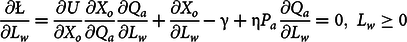 $${{\partial {\rm\Lstrok} {\rm{}}} \over {\partial {L_w}}} = {{\partial U} \over {\partial {X_o}}}{{\partial {X_o}} \over {\partial {Q_a}}}{{\partial {Q_a}} \over {\partial {L_w}}} + {{\partial {X_o}} \over {\partial {L_w}}} - {\rm{\gamma }} + {\rm{\eta }}{P_a}{{\partial {Q_a}} \over {\partial {L_w}}} = 0, \ {L_w} \ge 0$$
 $${{\partial {\rm\Lstrok} {\rm{}}} \over {\partial {L_r}}} = {{\partial U} \over {\partial {X_o}}}{{\partial {X_o}} \over {\partial {Q_a}}}{{\partial {Q_a}} \over {\partial {L_r}}} + {{\partial {X_o}} \over {\partial {L_r}}} - {\rm{\gamma }} + {\rm{\eta }}{P_a}{{\partial {Q_a}} \over {\partial {L_r}}} = 0, \ {L_r} \ge 0$$
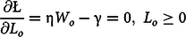 $${{\partial {\rm\Lstrok} {\rm{}}} \over {\partial {L_o}}} = {\rm{\eta }}{W_o} - {\rm{\gamma }} = 0, \ {L_o} \ge 0$$
 $${{\partial {\rm\Lstrok} {\rm{}}} \over {\partial {L_l}}} = {{\partial U} \over {\partial {X_o}}}{{\partial {X_o}} \over {\partial {L_l}}} - {\rm{\gamma }} = 0, \ {L_l} \gt 0$$
 $${{\partial {\rm\Lstrok} {\rm{}}} \over {\partial X}} = {{\partial U} \over {\partial {X_o}}}{{\partial {X_o}} \over {\partial {Q_a}}}{{\partial {Q_a}} \over {\partial X}} + {\rm{\eta }}{P_a}{{\partial {Q_a}} \over {\partial X}} - \eta {P_x} = 0, X \ge 0$$
 $${{\partial {\rm\Lstrok} {\rm{}}} \over {\partial {X_m}}} = {{\partial U} \over {\partial {X_m}}} - \eta {P_m} = 0, {X_m} \gt 0 .$$
 Equations (8)–(13) show how the household allocates its time for crop farming, searching for grazing land and water, collecting crop residue, and off-farm and leisure activity. For instance, if the household spends time searching for grazing land,Footnote 4L g > 0, the Khun-Tucker first-order condition indicates that  ${{\partial {\rm\Lstrok} {\rm{}}} \over {\partial {L_g}}} = 0.$ Thus, equation (9) becomes
 $${{\partial {X_o}} \over {\partial {L_g}}} = {\rm{\gamma }} - {{\partial {Q_a}} \over {\partial {L_g}}}\left( {{{\partial {X_o}} \over {\partial {Q_a}}} + {\rm{\eta }}{P_a}} \right).$$
 In this equation, the left part shows the value of marginal utility of the household from consumption of own goods—meals prepared from own crop grain and animal goods such as milk and meat coming from animals whose source of feed is the scarce grazing land. For an inequality constraint,  ${\rm{\gamma }}$ and ${\rm{\eta }}$ represent nonnegative Lagrangian multipliers for the time constraint and full income constraints. The local agricultural output market price, P a, is positive. The marginal utility derived from the consumption of own goods, which comes from the increased agricultural output $\left( {{{\partial {X_o}} \over {\partial {Q_a}}}} \right)$, is also assumed to be nonnegative. The right-hand side of equation (16) becomes positive if the marginal effect of using labor searching for grazing land on the agricultural output $\left( {{{\partial {Q_a}} \over {\partial {L_g}}}} \right)$ is negative. This implies that the right-hand side of equation (16) represents the marginal effect of spending labor searching for grazing land in terms of lower agricultural products and the extra negative burden it imposes on households’ time and budget constraints γ and η.
Equation (16) states that households allocate labor time for reaching grazing land until the marginal utility of labor used for grazing equals the marginal cost of household labor. If we use the first-order conditions for searching water or collecting crop residues, instead of grazing land, a similar result to that of equation (16) will follow. The main question that interests us is whether the scarcity of these resources adversely affects crop production. The hypothesis to be tested is that farmers that spend more time on searching for these scarce resources are likely to be less productive in crop production—that is, we test whether  ${{\partial {Q_a}} \over {\partial {L_g}}} \lt 0$ , or ${\rm{}}{{\partial {Q_a}} \over {\partial {L_w}}} \lt 0$, or ${{\partial {Q_a}} \over {\partial {L_r}}} \lt 0$ using level and shadow valuesFootnote 5 of these resources as an indicator of scarcity in the study area.
3. Empirical review
The well-being of Ethiopians heavily depends on farm and rangeland, water, and climatic resources because of the dependence of the majority of the Ethiopian people on subsistence agriculture. The increasing scarcity of these resources means increasing searching and collection times (Guarascio et al., Reference Guarascio, Gunewardena, Holding-Anyonge, Kaaria, Stloukal, Sijapati Basnett and Degrande2013). Rural households face trade-offs in the allocation of labor time between crop production and searching for or collecting resources for energy use and feeding animals (Mekonnen et al., Reference Mekonnen, Bryan, Alemu and Ringler2017). Shrinking access to scarce resources near the home, which is becoming a pressing reality in many developing countries, and the time taken to search for and collect them often imply that farmers have less time left for other activities. This adds to the labor burden of women, as traditional roles such as raising children and cooking make women often work much longer hours than their male spouses (Kes and Swaminathan, Reference Kes, Swaminathan, Blackden and Wodon2006; Wan, Colfer, and Powell, Reference Wan, Colfer and Powell2011). It has been commonly understood that children and women are mostly responsible for feeding and watering animals and that the scarcity of these resources increases the burden on these household members.
Herders, mostly boys, frequently travel long distances with animals in search of feed and water when feed scarcity increases household members’ and livestock mobility (Tangka and Jabbar, Reference Tangka and Jabbar2005). Likewise, when the distances become too long for resource collection on foot, men tend to assume the role of resource collection and transportation using donkey carts and small trucks (Sunderland et al., Reference Sunderland, Achdiawan, Angelsen, Babigumira, Ickowitz, Paumgarten, Reyes-García and Shively2014). Thus, increased competition on household members’ time between herding and cropping may result in lower livestock productivity and crop productivity (Tangka and Jabbar, Reference Tangka and Jabbar2005; Wan, Colfer, and Powell, Reference Wan, Colfer and Powell2011). The overall effect of feed scarcity is lower livestock income from the sale of livestock and livestock products, reduced access to food, increased labor burden of all household members, and reduced food and nutrition security for human welfare (Tangka and Jabbar, Reference Tangka and Jabbar2005).
Increasing resource scarcity has economic implications for poor rural households. One potential effect for concern is declining agricultural output as a result of reallocating inputs away from agriculture. The pioneering study by Cooke (Reference Cooke1998a) revealed that a reallocation of time away from farm work occurs as natural resources become scarcer in Nepal. The work of Kumar and Hotchkiss (Reference Kumar and Hotchkiss1988) also found that time spent in crop farming declines with a higher degree of fuelwood scarcity. The findings of Tangka and Jabbar (Reference Tangka and Jabbar2005) in Kenya show that feed scarcity increases livestock traveling distances in search of feed and water, resulting in lower livestock and crop output by increasing households’ time for collection. Likewise, Cooke, Köhlin, and Hyde (Reference Cooke, Köhlin and Hyde2008) explained the effect of forest scarcity on the livelihood of rural people in Nepal and found negative effects on agriculture.
Bandyopadhyay, Shyamsundar, and Baccini (Reference Bandyopadhyay, Shyamsundar and Baccini2011) found that more time spent on scarce fuelwood was associated with negative welfare in Malawi. Another related study by Damte, Koch, and Mekonnen (Reference Damte, Koch and Mekonnen2011) in Ethiopia indicated that rural households respond positively to fuelwood shortages by increasing their labor input. Mekonnen, Damte, and Deribe (Reference Mekonnen, Damte and Deribe2015) show that fuelwood scarcity has a negative and significant impact on time spent on agriculture. Similarly, Mekonnen et al. (Reference Mekonnen, Bryan, Alemu and Ringler2017) concluded that agricultural productivity decreases with increasing time spent on collecting animal dung but increases with time spent on collecting crop residue. From the previous brief review of related works, we note that the evidence on the effect of natural resource scarcity on agricultural output is, unfortunately, sparse.
There are two methods of scarcity measures in the literature on resource scarcity: physical measures and economic measures. Physical measures include distance from the resource (fuelwood, water, grazing, and fodder) or village-level availability of these resources (as applied by Cooke, Reference Cooke1998a, Reference Cooke1998b; Cooke, Köhlin, and Hyde, Reference Cooke, Köhlin and Hyde2008; Damte, Koch, and Mekonnen, Reference Damte, Koch and Mekonnen2011; Hadush, Reference Hadush2018; Mekonnen, Damte, and Deribe, Reference Mekonnen, Damte and Deribe2015; Mekonnen et al., Reference Mekonnen, Bryan, Alemu and Ringler2017; Veld et al., Reference Veld, Narain, Gupta, Chopra and Singh2006). However, labor shortages in rural areas are often more important for household fuelwood-use decisions than the physical scarcity of fuelwood. This means that physical measure is not a reliable indicator of resource scarcity. The opportunity cost of the time spent searching or collecting is, therefore, considered to be a better measure (Cooke, Köhlin, and Hyde, Reference Cooke, Köhlin and Hyde2008; Damte, Koch, and Mekonnen, Reference Damte, Koch and Mekonnen2011). The name of the opportunity cost is interchangeably known as shadow price or shadow cost of resources and can, therefore, be different from the market price (Strauss, Reference Strauss, Singh, Squire and Strauss1986).
As demonstrated (Baland et al., Reference Baland, Bardhan, Das, Mookherjee and Sarkar2010; Cooke, Reference Cooke1998a, Reference Cooke1998b; Hadush, Reference Hadush2018; Mekonnen, Reference Mekonnen1999; Mekonnen, Damte, and Deribe, Reference Mekonnen, Damte and Deribe2015; Murphy, Berazneva, and Lee, Reference Murphy, Berazneva and Lee2015), the opportunity cost is commonly approximated in two ways. First, it is the wage rate multiplied by the time spent per unit of environmental good collection, as a measure of scarcity, and second, as the marginal product of labor in resource collection multiplied by the shadow wage. Besides, shadow wage or shadow price is calculated by the ratio of predicted outputs to labor time multiplied by the coefficient of labor derived from the Cobb-Douglas production function (Jacoby, Reference Jacoby1993; Le, Reference Le2010). Because of missing data for the estimation of the economic scarcity, which requires an exclusion restriction, we mainly use the physical indicators of scarcity for our inference. Regarding this subject and method, evidence from Africa is scarcer in the existing studies. Hence, this article will contribute to the sparse empirical evidence from sub-Saharan Africa (Cooke, Köhlin, and Hyde, Reference Cooke, Köhlin and Hyde2008; Khan, Reference Khan2008) by exclusively analyzing the economic effect of these scarce resources on household labor input and crop production.
4. Study area and data description
The study is conducted in the Tigrai region, the northern part of Ethiopia. It is based on cross-sectional survey data from NMBU-MU collected in 2015 from 632 sample households. The dataFootnote 6 include a panel of five rounds conducted in 1997–1998, 2000–2001, 2002–2003, 2005–2006, and 2014–2015 where the author was involved only in collecting the data for the last round. Initially, to reflect systematic variation in agroclimatic conditions, agricultural potential, population density, and market access conditions, four communities from each of the four zones were selected, and three communities that represent irrigation projects were also chosen. Likewise, one with low population density and one with high population density were strategically selected from each zone among these communities to reflect distance from the market (Hagos, Reference Hagos2003).
This article uses only cross-sectional data for 2015 extracted from the survey for the simple reason that some outcome and explanatory variables were only added in the last round. For this study, the need for information regarding livestock activity restricted us to use only 518 livestock owner-farmers. Table 1 presents the basic socioeconomic characteristics of the 518 farm households. The first dependent variable in this article is labor time for crop farming. For the sake of reliable estimation, 16 distorting observations or outliers were dropped from the data set in this estimation. The second dependent variable is aggregate household agricultural production or monetary value of all crops produced during the survey production season. Following Jacoby (Reference Jacoby1993), Klemick (Reference Klemick2011), and Gutu (Reference Gutu2016), multiple crop outputs are aggregated into a single output measure using the medians of self-reported village prices within each village.
Table 1. Descriptive and summary statistics

a Includes the value of crop, fruit, and vegetable production in ETB.
b Includes income from agriculture, off-farm, transfer, and safety net.
c One tsmdi is approximately one-quarter hectare.
d Total monetary value of all farm implements such as plough parts, hoe, cart, sickle, and spade.
Note: ETB, Ethiopian birr; masl, meters above sea level; TLU, tropical livestock unit.
In this case, nine distorting observations and outliers were dropped from the data set to have a reliable estimation. An average household owns production farm capital tools worth about ETBFootnote 7 639 and produced an average agricultural output worth ETB 41,645 in the survey year, with an average total income including livestock, off-farm, transfer, and business to be ETB 49,426. Besides, on average each household spent 683.6 labor hours for crop production during the planting and harvesting season, and about 274 labor hours were allocated to livestock rearing excluding child labor time for the same seasons.
Straw has a local market price and is therefore relatively easy to value. Grazing land and water, on the other hand, are difficult to value because they are not traded and have no market price; thus, their prices are shadow prices (Magnan, Larson, and Taylor, Reference Magnan, Larson and Taylor2012). Shadow prices/shadow costs are assumed to reflect better the economic scarcity of environmental goods to a household (Cooke, Reference Cooke1998a). For this reason, first, we use walking time to measure grazing, water, and crop residue using a similar method as that used by Palmer and MacGregor (Reference Palmer and MacGregor2009) and Amacher, Hyde, and Joshee (Reference Amacher, Hyde and Joshee1993) as a proxy indicator of the scarcity of these resources. On average, the households spend 1.25 hours to reach a water source for animals and 1.31 hours to search for communal grazing land daily for a single trip, with the maximum time reaching up to 6 hours for water sites and 8 hours for grazing land in the data. Besides, the average time spent on collecting straw by the households is 9.6 hours, ranging from a minimum value of 0.3 to a maximum value of 100 hours per collecting season.
Second, following Cooke (Reference Cooke1998a, Reference Cooke1998b), Damte, Koch, and Mekonnen (Reference Damte, Koch and Mekonnen2011), Baland et al. (Reference Baland, Bardhan, Das, Mookherjee and Sarkar2010), Mekonnen, Damte, and Deribe (Reference Mekonnen, Damte and Deribe2015), and Hadush (Reference Hadush2018), we measure the shadow costs of natural resources (grazing and water) and collecting crop residue as the time taken to reach grazing land and water sites or to collect crop residue per its amount collected multiplied by the village adjustedFootnote 8 off-farm wage. In this article, we take the wage rate for those who report working for an off-farm wage in the local labor market, and the wages for those who did not report working were missing but imputed following Heckman’s (Reference Heckman1979) two-stage approach as is applied by Cooke (Reference Cooke1998a, Reference Cooke1998b).
In this way, we produce a household-specific shadow price/shadow cost of searching for grazing land or water and collecting straw. Using these data in Table 1, the average shadow price/shadow cost for animal watering is about ETB 147 per day, which is equivalent to the average daily rural wage rate in the region. On average, the shadow price of searching for grazing land is ETB 205 per day, which is greater than the shadow price of water and straw. This is not surprising, as rural farmers usually spend more labor time in searching for grazing land than watering. As expected, the shadow price of collecting straw is ETB 12 per trip. This is a small value compared with the value on grazing and water, reflecting the reality that collecting straw requires less time than the time taken up by grazing and watering activities.
5. Empirical model specification
This article draws on the AHM, which provides a holistic framework to analyze the economic effect of resource scarcity on labor to crop farming and the monetary value of crop production in the farm household. Based on the reduced form equations derived from AHM, we first model labor allocation to crop farming as a function of resource scarcity and household characteristics following Cooke (Reference Cooke1998a) and Mekonnen, Damte, and Deribe (Reference Mekonnen, Damte and Deribe2015). We estimate the effect of resource scarcity ( ${L_i}$) on time spent in crop farming (L a) using ordinary least squares (OLS) on log-log function. The labor input allocated to crop farming activity ( ${L_a})$ is influenced mainly by the time spent on looking for grazing lands and water (L g, L w) and collecting straw (L r) represented by L i. The labor input allocation of households also depends on the vector of household and community characteristics (Xi). Given that e 1 is the error term, the labor input allocation model is easily specified as
 $$\ln {L_a}{\rm{}} = {\alpha _0} + {\alpha _i}\ln {L_i} + {\beta _i}{X_i} + {e_1}.$$
The choice of functional form for the estimation of the monetary value of crop production function with respect to different inputs has gained substantial attention in the economic literature. With regard to estimation, the production function is mostly estimated using the Cobb-Douglas production function because the output is a simple function of labor and capital. However, this does not allow other variables than just the two that can significantly affect production such as fertilizer and land. For this reason, the GCD production function developed by Diewert (Reference Diewert1973) was adopted to incorporate these variables into the production function.
The GCD production function that satisfies the nonnegative, nondecreasing, continuous, and quasiconcave properties of the standard production function is denoted by
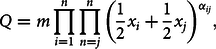 $$Q = m\mathop \prod \limits_{i = 1}^n \mathop \prod \limits_{n = j}^n {\left( {{1 \over 2}{x_i} + {1 \over 2}{x_j}} \right)^{{\alpha _{ij}}}},$$
where Q is output in the aggregate monetary value of crop production, x 1, …, x n are quantities of the n inputs of production and not the negative inputs of production, m > 0, αij = α ji, and  $\mathop \sum \nolimits_{i = 1}^n \mathop \sum \nolimits_{j = 1}^{n} {\alpha _{ij}} = 1$ (this is the assumption of a constant return to scale). Assuming that α ij = 0 for all i ≠ j and taking the natural log of equation (18) produces a standard Cobb-Douglas equation with many inputs, which is to be estimated in its natural log form:
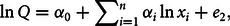 $$\ln Q{\rm{}} = {\alpha _0} + \mathop \sum \nolimits_{i = 1}^n {\alpha _i}\ln {x_i} + {e_2},$$
where α 0 = ln m (m is the constant term in equation 18, and e 2 is the error term). The GCD production function is often criticized for being restrictive because of its assumptions of constant returns to scale (CRTS). It also assumes perfect competition in both input market and output market even if it can handle a large number of inputs. Its assumptions make it difficult to measure technical efficiency levels and growth effectively. However, the assumption about the market does not significantly affect the estimation power of the Cobb-Douglas production function as long as factors are paid according to their relative shares (Murthy, Reference Murthy2002). Besides, Miller (Reference Miller2008) argued that GCD can be estimated by relaxing the CRTS assumption and then test whether the summation of the coefficients is significantly different from one using the standard econometric procedure. The author noticed that this empirical model does not address the issue of reverse causality and endogeneity related to time use because of a lack of proper instruments for time use. Therefore, care is taken with its interpretation.
In the case of computing shadow costs of grazing, water, and straw, we used imputed wages for those who reported to be nonemployee households. It has been popular to impute wages of nonemployed persons from the wage equation, which describes the functional relationship between wage and personal characteristics such as age, marital status, place of living, work experience, and occupation. The wage equation is typically modeled within the linear regression model and estimated using the sample of employed persons. However, such an approach, which uses only data on employed persons, was criticized by Heckman (Reference Heckman1979). He suggested the two-stage model, consisting of a wage equation and a participation equation, in which the latter estimates the probability of a person to be employed versus nonemployed. This has been popular among researchers and widely applied for prediction of wages of nonemployed persons and estimation of the gender wage gap (for details, see Breunig and Mercante, Reference Breunig and Mercante2010; Labeaga, Oliver, and Spadaro, Reference Labeaga, Oliver and Spadaro2008). This study did not address the issue of reverse causality and endogeneity related to time use because of a lack of proper instruments for time use. It rather treated them as exogenous following the work of Cooke (Reference Cooke1998a), Cooke, Köhlin, and Hyde (Reference Cooke, Köhlin and Hyde2008), Hadush (Reference Hadush2018), and Mekonnen, Damte, and Deribe (Reference Mekonnen, Damte and Deribe2015).
In order to test for separability (i.e., whether the labor market or straw market functions well), we examined the relationship between the estimated shadow wages/price (shadowV) and market wages/prices (marketV) reported by the households that participate in off-farm or straw market using a similar method as that used by Jacoby (Reference Jacoby1993) and Skoufias (Reference Skoufias1994). The regression is specified as
 $$shadowV = {\beta _0} + {\beta _1}marketV + \varepsilon ,$$
where  $shadowV = Q/D \times {\delta _L}$, which represents shadow wage or shadow price calculated by the ratio of predicted outputs (Q) to labor time (D) multiplied by the coefficient of labor derived from the Cobb-Douglas production function following Jacoby (Reference Jacoby1993) and Le (Reference Le2010). The test for the straw market is whether β 0 = 0 and β 1 = 1; under the null, the market price reflects the value of the marginal product of labor or straw.
6. Empirical results and discussions
6.1. Resource scarcity and labor time for crop farming
What are the consequences of increasing grazing, water, and straw scarcity for crop labor input? We answer this question by examining the link between resource scarcity and labor input to crop farming in rural areas of Ethiopia using similar estimation methods as in Cooke (Reference Cooke1998a). In this article, the main variables of greatest interest are water for animal and feed scarcity measured by the time taken to reach them. A priori, animal water and feed scarcity should reduce labor time on the crop farm because they take away time from crop farms and leisure as people search for these resources. Using OLS on log-log function, the estimate of the effect of resource scarcity on time spent in crop farming is presented in Table 2. Given that coefficients of the resource variables have similar magnitudes to the result of single regression in the case of separate estimation, we just prefer to control them in a single estimation unlike that of crop output value estimation. For the sake of reliable estimation, 16 distorting observations or outliers were dropped from the data set in this estimation.
Table 2. Estimation of household labor allocation to crop farming

a The difference between the first and second column is that the second estimation is based on the level value of family labor and level value of resource scarcity indicators (time taken to reach grazing, water, and straw sites measured in hours).
Notes: Asterisks (***, **, and *) indicate that the estimated parameters are significantly different from zero at the 1%, 5%, and 10% significance levels, respectively. Numbers in parentheses are standard errors. ETB, Ethiopian birr; TLU, tropical livestock unit.
Our results do support the hypothesis of a negative relationship between total household labor allocation to crop farming and resource scarcity at the household level. With respect to the variables of interest, higher searching time for water and grazing and collecting straw were shown to significantly reduce labor time to crop farming. We found that a 1% increase in searching time for water and grazing and collecting straw results in 0.06%, 0.09%, and 0.10% decrease in time spent on crop farming, respectively. Using level values in linear regression, we also found that increasing time spent to reach water, grazing, and straw sites by 1 hour led to a decrease in crop farm labor of 10.8 hours, 9.7 hours, and 2 hours, respectively. This result finds favor among several researchers (Bandyopadhyay, Shyamsundar, and Baccini, Reference Bandyopadhyay, Shyamsundar and Baccini2011; Cooke, Reference Cooke1998a; Cooke, Köhlin, and Hyde, Reference Cooke, Köhlin and Hyde2008; Mekonnen, Damte, and Deribe, Reference Mekonnen, Damte and Deribe2015). We found significant effects of other covariates as well. Land area in crops has a significant positive correlation with total household labor input to farming. The real off-farm wage has a significant positive effect on household farm labor input.
As expected, we also found that large family households spend more time per person on crop farming. The households living in lowland areas spend more farm labor input to farming than their counterparts. Wealthier households that have more livestock spend more time for farming. Higher on-farm income is associated with households’ greater time input to crop farming. Hiring labor from the local market decreases family labor input to farming, and farmers living at high altitude tend to allocate more labor input to crop farming. These findings correspond to the results of previous studies by Cooke (Reference Cooke1998a), Okwi and Muhumuza (Reference Okwi and Muhumuza2010), Bandyopadhyay et al. (Reference Bandyopadhyay, Shyamsundar and Baccini2011).
6.2. Resource scarcity and monetary value of aggregate crop production
For the sake of reliable estimation, outliers are removed from the data set. Thus, nine distorting observations were dropped from the data set in food production estimation. In order to estimate the production sector of the farm households, we used OLS on the log-transformed form of the GCD production function specified in Section 5. The dependent variable is the monetary sum of all crops produced during the survey harvesting season. The estimates of the production function using walking distance and shadow values of water, grazing land, and straw are presented in Tables 3 and 4. In general, the estimation shows that all explanatory variables exhibit significant and theoretically expected signs.
Table 3. Ordinary least squares estimation of log monetary value of aggregate agricultural production

Notes: Asterisks (***, **, and *) indicate that the estimated parameters are significantly different from zero at the 1%, 5%, and 10% significance levels, respectively. Numbers in parentheses are standard errors.
Table 4. Ordinary least squares estimation of log monetary value of aggregate agricultural production

Notes: Asterisks (***, **, and *) indicate that the estimated parameters are significantly different from zero at the 1%, 5%, and 10% significance levels, respectively. Numbers in parentheses are standard errors.
Variables of interest in this article are time spent on looking for water and feed resources included so as to capture the effect of resource scarcity on agricultural production. The second column of Table 3 presents the estimation of log output with water scarcity taken into account, as do the second and the third columns, putting grazing land and straw collection into consideration. The results are in favor of our hypothesis. As expected, column 2 of Table 3 indicated that time spent on searching for water for animals is found to be negative and significant, suggesting that a 1% increase in time spent looking for water decreases crop production by 0.16%, and time spent on searching for grazing land has a stronger effect than this variable as shown in column 3 (i.e., a 1% increase in time spent searching for grazing land decreases agricultural output by 0.28%). Another scarcity-related variable is time spent for collecting straw, which significantly resulted in a negative sign, implying that farmers that spend 1% additional time collecting straw produce about 0.33% less output (column 4). The output effect obtained here supports the claim that time spent searching for scarce resources displaces labor time from production activity and hence reduces output (Cooke, Köhlin, and Hyde, Reference Cooke, Köhlin and Hyde2008; Damte, Koch, and Mekonnen, Reference Damte, Koch and Mekonnen2011; Mekonnen, Damte, and Deribe, Reference Mekonnen, Damte and Deribe2015; Tangka and Jabbar, Reference Tangka and Jabbar2005).
The estimated coefficient for land (0.29, 0.30, and 0.20) shows that when landholding increases by 1%, agricultural production increases, on average, by 0.3%, implying that land is a vital input for agriculture. The result is similar to the findings of Sarris, Savastano, and Christiaensen (Reference Sarris, Savastano and Christiaensen2006) in Tanzania. As expected, fertilizer and manure use are found to be significant and positive variables indicating that a 1% increase in fertilizer and manure use, respectively, leads to a 0.15% and 0.09% increase in agricultural outputs in line with the studies conducted by Demeke, Keil, and Zeller (Reference Demeke, Keil and Zeller2011) and Di Falco, Veronesi, and Yesuf (Reference Di Falco, Veronesi and Yesuf2011), whose results revealed that fertilizer and manure use positively and significantly affected food production in Ethiopia. In Ethiopia, an ox is the main capital input and can be considered an equivalent substitute for the uses of a tractor. In this article, the number of oxen owned is significant, leading to a 0.23% increase in the agricultural output. A similar result was reflected by Mekonnen, Damte, and Deribe (Reference Mekonnen, Damte and Deribe2015) who found a positive effect of ox input on food crop productivity in Ethiopia.
In line with the predictions of economic theory, labor is positively and statistically significant. A 1% increase in man-day labor causes farm output to increase by about 0.35%, a finding that is consistent with the notion that labor has a positive effect on production (Abdulai and Huffman, Reference Abdulai and Huffman2014; Di Falco, Veronesi, and Yesuf, Reference Di Falco, Veronesi and Yesuf2011), but the coefficient on seed input contradicts the findings by Di Falco, Veronesi, and Yesuf (Reference Di Falco, Veronesi and Yesuf2011) in Ethiopia and Bulte et al. (Reference Bulte, Beekman, Di Falco, Hella and Lei2014) in Tanzania. Farmers hiring extra labor seem to increase their production value by 0.48%. Another capital input included in the analysis is production capital, which is the monetary value of farm tools. A 1% increase in production capital can increase agricultural output by 0.06%. This finding supports an earlier study by Sarris, Savastano, and Christiaensen (Reference Sarris, Savastano and Christiaensen2006).
Not surprisingly, we found that an increase in shock has quite a large detrimental effect on food production (–2.16%), which is consistent with a previous study by Abdulai and Huffman (Reference Abdulai and Huffman2014), who confirmed a negative effect of drought or illness shock on production. The variable representing education of the household head is positive and significantly different from zero, suggesting that education plays an important role in producing more, which is in agreement with Abdulai and Huffman’s (Reference Abdulai and Huffman2014) results.
For comparison purposes, the estimates of the effect of this resource scarcity on crop output value are presented in Table 4 using their shadow prices. In line with our expectation, we found that water scarcity reduces crop output value. The results suggest that a 1% increase in the shadow price of water for animals results in a 0.08% decrease in agricultural output value. The effect is lower as compared with the effect of the distance value in Table 3. Agricultural crop value also decreases as the shadow price for grazing land increases; on average, a rise of 1% in the shadow price of reaching grazing land implies a fall of 0.09% in crop output produced. The significant and large effect of grazing scarcity on crop output is because farmers with a large number of cattle require more labor time to search for animal pasture.
The coefficient on the shadow price of collecting straw indicates that a 1% increase in shadow price reduces crop output by 0.15%. This is consistent with the idea that the potential effect of scarce resources is declining agricultural output as a result of reallocating inputs away from agriculture (Cooke, Köhlin, and Hyde, Reference Cooke, Köhlin and Hyde2008; Mekonnen, Damte, and Deribe, Reference Mekonnen, Damte and Deribe2015; Mekonnen et al., Reference Mekonnen, Bryan, Alemu and Ringler2017), which further supports the downward spiral hypothesis that resource degradation leads to poverty (Yang, Utzinger, and Zhou, Reference Yang, Utzinger and Zhou2015).
While Tables 3 and 4 present results in a log value or percentage form, Table 5 reports linear-linear estimation of output between the crop output value and resource scarcity using level values. The justification is that the level value using currency value is direct and easier to interpret than the percentage value forms. This estimation has been done mainly for checking consistency and examining the gender differential resource scarcity effect on the crop output value. For brevity, only coefficients of variables of interest are interpreted here. The results across the three columns (full sample, male, and female) and different estimators are quite similar (Table 5). An increase of 1 hour in the traveling time to water and grazing sites for animals leads to a decrease in the crop output value of ETB 171 and ETB 189, respectively. Likewise, an increase of ETB 24 in the crop production value is associated with a 1-hour reduction in straw collecting time, which is in favor of the findings of Cooke, Köhlin, and Hyde (Reference Cooke, Köhlin and Hyde2008) and Mekonnen et al. (Reference Mekonnen, Bryan, Alemu and Ringler2017).
Table 5. Ordinary least squares estimation of monetary value of aggregate agricultural production

Notes: Asterisks (***, **, and *) indicate that the estimated parameters are significantly different from zero at the 1%, 5%, and 10% significance levels, respectively. Numbers in parentheses are standard errors.
Table 5 further provides disaggregate analysis by gender. When we disaggregate the data by gender, we find out that an hour reduction in the traveling time to water sites for animals increases crop output value by about ETB 180 for male-headed households and ETB 157 for female-headed households, while the coefficient of grazing signals a decrease of ETB 207 for male-headed households and ETB 141 for female-headed households as a result of a 1-hour reduction in searching time for grazing. Our results also show that a decrease in straw collecting time is associated with a significant increase in the crop output value of ETB 25 for male-headed households and ETB 22 for female-headed households. The coefficients in all cases are negative, similar to findings in other studies (Gbetnkom, Reference Gbetnkom2007; Sunderland et al., Reference Sunderland, Achdiawan, Angelsen, Babigumira, Ickowitz, Paumgarten, Reyes-García and Shively2014; Tangka and Jabbar, Reference Tangka and Jabbar2005; Wan, Colfer, and Powell, Reference Wan, Colfer and Powell2011).
The finding is consistent with reality in the study area that herders, mostly boys, frequently travel long distances, with animals in search of feed and water when feed scarcity increases household members’ and livestock mobility. Likewise, when the distances become too great for resource collection on foot, men tend to assume the role of resource collection and transportation using donkey carts and small trucks. In line with this, Nahusenay and Tessfaye (Reference Nahusenay and Tessfaye2015) tried to examine labor allocation of family members arranged for watering and feeding and their result indicated that in the study area, adult males spent 57% of their time feeding animals, while adult females allocated 25% of their time to feeding animals.
An alternative is to estimate quantile regressions on farm output in order to capture the effects of these scarce variables across the entire distribution of the dependent variable (Koenker and Bassett, Reference Koenker and Bassett1978). Table 6 indicates that the elasticity values associated with a 1% change in distance to water on food products range from –0.16% for the second bottom quantile to –0.13% for the top quantile with a median value of –0.18%, resulting in an overall reduction of 0.18% in food production. The median distance to the grazing land elasticity of food production is –0.23%. For those in the 10th category of the food output distribution, a reduction in grazing distance could increase their output by about 0.22%, reaching a maximum effect of 0.45% for those in the last top quantile. Finally, the time spent for straw collection elasticity of food output is –0.26% at the median value but ranges from –0.23% for the 10th to –0.48% for the 100th as shown in Table 6. Similar results are found using shadow values in Table 6. This is evidence that estimating the quantile model gives more information than a single coefficient from OLS for both policy and inference cases.
Table 6. Effect of water, grazing, and feed scarcity on log output using quintile regression

Notes: Asterisks (***, **, and *) indicate that the estimated parameters are significantly different from zero at the 1%, 5%, and 10% significance levels, respectively. Numbers in parentheses are standard errors.
We report the results of tests of separability in Table 7, which are obtained from the regression of the form. The results strongly reject the existence of separability, implying that the estimated shadow wage/prices are a more accurate basis for understanding farming decisions in a rural area.
Table 7. The Jacoby test of separability with dependent variable: log (shadow wage/price)

Notes: Asterisks (***, **, and *) indicate that the estimated parameters are significantly different from zero at the 1%, 5%, and 10% significance levels, respectively. Numbers in parentheses are standard errors. OLS, ordinary least squares.
7. Conclusion and policy implications
In rural farms, households spend a large share of their daily time on searching for animal grazing and water, as well as collecting crop residue. This directly affects farm production by displacing labor from production activity. This study analyzes the economic implications of animal water and feed scarcity on labor farming and farm production in North Ethiopia using a nonseparable agricultural farm household model. To address our objectives, a GCD production function was estimated using a unique data set from 518 sample farmers.
The results of this study provide an interesting picture of smallholders in Ethiopia. As expected, it appears that time spent searching for animal water and feed has a significant and negative effect on labor and crop output. Our results confirm a negative relationship between labor input to crop farming and resource scarcity. We found that a 1% increase in searching time for water and grazing and collecting straw results in, respectively, a 0.059%, 0.092%, and 0.099% decrease in time spent on a crop farm. We also found that increasing time spent to reach water, grazing, and straw sites by an hour lead to a decrease in crop farm labor by 10.8 hours, 9.7 hours, and 2 hours, respectively, using level values in linear-linear model estimation.
In aggregate, reducing the time spent looking for water and grazing by 1% leads to an increase in food production by 0.16% and 0.28%, respectively, and an increment of 0.33% in food production is achieved by a 1% reduction in straw collecting time. Similarly, the shadow price variables are significant, have the expected negative sign, and are consistent with the theoretical predictions in that reduction of 0.074%, 0.094%, and 0.154% in crop output are reported by a 1% increase in the shadow price of water, grazing, and straw, respectively.
Using level values, increasing the traveling time to water, grazing, and straw sites for an animal by 1 hour leads to a decrease in a crop output value of ETB 171, ETB 189, and ETB 24, respectively. When we disaggregate the data by gender, we find that an hour reduction in searching time of scarce resource increases crop output value by about ETB 180 for male-headed households and ETB 157 for female-headed households in the case of water and by about ETB 207 for male-headed households and ETB 141 for female-headed households in the case of grazing. An increase in crop output value of ETB 25 for male-headed households and ETB 22 for female-headed households is also associated with a 1-hour decrease in the straw collecting time. Depending on results from the quantile regression, the effect of water and feed scarcity is not uniform across the food production distribution.
In general, this study can be helpful for policy makers working to alleviate animal water and feed problems in Ethiopia to justify their actions with empirical results. Based on the empirical results presented, two relevant areas of policy interventions can emerge: The first involves policies that facilitate easier access to a water tap for animals by advocating for emergency relief projects by the local government and nongovernment development agents. Then, this requires moving from owning a large quantity of less productive animals to owning few but productive animal breeds because livestock and population density are major causes of resource scarcity. This finding further indicates that the tragedy of the commons problem is not only limited to the herder’s problem but also affects crop producers in the case of smallholder farmers.
The second area of policy intervention involves the introduction of a more efficient animal feed management strategy with new livestock technologies such as the adoption of improved cows, by-products, fattening, and stall-feeding practices that improve cattle production and reduce land degradation, which is the primary cause of resource scarcity. Given the evidence in this article, it appears that policies that seek to promote literacy programs about how to optimally allocate daily time to livestock feeding and hence reduce negative effects on crop farming would be useful in enhancing household-level food security. This study did not address the link between resource scarcity and welfare using panel data to reflect the dynamic effect of resource scarcity. Further research should focus on adopting an approach using welfare indicators and longitudinal data in the same study area. Finally, the article does not address the issue of reverse causality and endogeneity related to time use because of a lack of proper instruments for time use. Therefore, a rigorous estimation is required with proper instruments. Thus, our interpretations and inferences mainly depend on the estimation of physical distance measures rather than shadow cost measures.
Acknowledgments
Special thanks go to my supervisor Professor Stein Holden (NMBU) for his unreserved advisorship, and coadvisor Dr. Mesfin Tilahun (MU) for his assistance.
Financial support
This research has been sponsored by the collaborative research and capacity-building project on Climate Smart Natural Resource Management and Policy (NORHED-CLISNARP) between Mekelle University and Norwegian University of Life Sciences. The NORHED-CLISNARP project and this research are funded by the Norwegian Agency for Development Cooperation (NORAD) and the Quota Scholarship program of StatensLånekasse for Utdanning.


 Open access