INTRODUCTION
Thoughtful irrigation water management and use of innovative agricultural technologies could help in devising long-term strategies for adaptation to climate change. Use of modern tools in water management and formulation of agricultural policies should be oriented towards enhancing water productivity in agriculture. This will not only save water but will also maintain food security in developing countries. Some predictive studies conducted so far and some hard evidence suggest that the variability in rainfall intensity and duration, as well as other climatic parameters due to climate change, are most likely to have adverse effects on agricultural production (Supit et al. Reference Supit, Van Diepen, De wit, Wolf, Kabat, Baruth and Ludwig2012; Berg et al. Reference Berg, De Noblet-ducoudré, Sultan, Lengaigne and Guimberteau2013; Ju et al. Reference Ju, Lin, Wheeler, Challinor and Jiang2013). Therefore, proper irrigation scheduling vis-à-vis the rainfall variability will ensure sustainable production of food grains with judicious water management and saving of water. To accomplish this objective, the real challenge lies in reliable prediction of future climate change and using it for the estimation of crop water requirements at different growth stages. Furthermore, water budgeting will quantify the amount and timing of irrigation in order to attain sustainability in the agricultural production of a region. Such linkage of climate generators with crop yield models could be useful for prediction of crop yield under changing climate scenarios in the future. Additionally, it will help in evaluating different crop management options to decide upon the best scenario for enhancing agricultural production under a given set of site-specific input parameters that affect crop yield.
Several researchers have studied linking climate predictions obtained from global circulation models (GCM) with crop models to estimate the future crop yield under different climate change scenarios (Baron et al. Reference Baron, Sultan, Balme, Sarr, Traore, Lebel, Janicot and Dingkuhn2005). Many have analysed historical climate and crop yield data to generate future scenarios of crop yield under changing climate conditions for different regions (Iglesias et al. Reference Iglesias, Rosenzweig and Pereira2000; Izaurralde et al. Reference Izaurralde, Rosenberg, Brown and Thomson2003; Tan & Shibasaki Reference Tan and Shibasaki2003; Parry et al. Reference Parry, Rosenzweig, Iglesias, Livermore and Fischer2004; Huntingford et al. Reference Huntingford, Lambert, Gash, Taylor and Challinor2005; Tao et al. Reference Tao, Yokozawa, Xu, Hayashi and Zhang2006; Anwar et al. Reference Anwar, O'leary, Mcneil, Hossain and Nelson2007; Challinor et al. Reference Challinor, Wheeler, Craufurd, Ferro and Stephenson2007; Tubiello & Fischer Reference Tubiello and Fischer2007; Egli Reference Egli2008; Thomas Reference Thomas2008; Malone et al. Reference Malone, Meek, Hatfield, Mann, Jaquis and Ma2009). Some researchers have used a climate generator such as ClimGen to forecast daily weather data for its subsequent use as input for a crop model to examine crop yield variations under changing climate (Stöckle et al. Reference Stöckle, Campbell and Nelson1997; Zhang & Liu Reference Zhang and Liu2005; Kou et al. Reference Kou, Ge, Wang and Zhang2007; Tao et al. Reference Tao, Hayashi, Zhang, Sakamoto and Yokozawa2008). Zhang et al. (Reference Zhang, Peng and Huang2004) used ClimGen to simulate daily climatic data of several weather stations across Canada and reported that by choosing appropriate scaling parameters, the ClimGen generated daily data were not statistically different from observed daily data for precipitation, maximum/minimum temperature and solar radiation. However, Zhang et al. (Reference Zhang, Peng and Huang2004) also observed that ClimGen generated data may not be accurate for the transitional periods between the spring and autumn seasons in Canada. Castellvi & Stöckle (Reference Castellvi and Stöckle2001) compared the performance of weather generator (WGEN) and ClimGen for generation of long-term weather data at seven different locations in Italy, representing variable climatic conditions, and observed that neither model was able to replicate the actual distribution over the entire range of values for maximum/minimum temperature, solar radiation and evapotranspiration. However, WGEN generated the monthly mean temperature more accurately and ClimGen predictions for daily temperature and solar radiation were better than WGEN. Stöckle et al. (Reference Stöckle, Donatelli and Nelson2003) evaluated weather data for calculating Penman–Monteith reference crop evapotranspiration using the ClimGen model: radiation and vapour pressure deficit (VPD) were estimated from temperature data and used to calculate evapotranspiration at five locations, representing tropical, temperate, semi-arid and arid climates. ClimGen was calibrated for each location using the most recent 2 or 5 years of daily weather records. Actual and estimated values were compared on a daily and weekly (7-day running average) basis. Analysis of reference crop evapotranspiration (ETo) totals for individual years confirmed that the two temperature-based methods were adequate to estimate Penman–Monteith ETo when calibrated for application in arid and semi-arid locations. Several attempts have been made to study the impacts of climate change on yield of maize at different locations around the world (viz. Muchena & Iglesias (Reference Muchena, Iglesias, Rosenzweig, Allen, Harper, Hollinger and Jones1995) in Zimbabwe, Delécolle et al. (Reference Delécolle, Ruget, Ripoche, Gosse, Rosenzweig, Allen, Harper, Hollinger and Jones1995) in France, Tubiello & Fischer (Reference Tubiello and Fischer2007) in Italy and Jones & Thornton (Reference Jones and Thornton2003) in Africa and Latin America. Castellvi & Stöckle (Reference Castellvi and Stöckle2001) generated weather data using ClimGen with three different generation methods and showed that the two-parameter Weibull distribution performed better than other methods in reproducing temperature and bright sunshine hours. McKague et al. (Reference Mckague, Rudra, Ogilvie, Ahmed and Gharabaghi2005) evaluated ClimGen for generation of daily precipitation, air temperature, solar radiation, wind speed and relative humidity for Southern Ontario, Canada. The comparison of simulated weather data with 30 years of weather data for six stations indicated that ClimGen performed with reasonable accuracy with some limitations in generating rainfall intensities and solar radiation, particularly for the winter months. M. G. Abraha (personal communication) reported that long-term weather data for precipitation, minimum/maximum air temperatures and solar radiation can be used in ClimGen to generate the climatic parameters for estimation of crops yield. Sarangi & Kumar (Reference Sarangi and Kumar2009) investigated a trend analysis of 36 years’ rainfall data from the Water Technology Centre (WTC) observatory of the Indian Agricultural Research Institute (IARI) and used ClimGen to predict the climate in future years (2010–2050). Furthermore, the generated data were used in the CROPWAT model to estimate irrigation water requirements for future years to obtain a sustainable yield of maize. It was observed that ClimGen was able to predict the climate data with acceptable accuracy and the linkage of ClimGen and CROPWAT enabled an estimation of future irrigation water requirements.
Geerts et al. (Reference Geerts, Raes and Garcia2010) used the AquaCrop model to simulate crop development for a long series of historical climate data and generated guidelines for deficit irrigation schedules to enhance crop water productivity of quinoa in Central Bolivian Altiplano. They developed a practical chart by combining AquaCrop in combination with long series of climate data and frequency analysis, for guiding deficit irrigation of quinoa after wet, normal or dry weather conditions during the vegetative growth stages. Erkossa et al. (Reference Erkossa, Menker and Betrie2011) used the AquaCrop model to estimate the yield and water productivity of wheat under the rainfed system on vertisols in the Ethiopian Highlands; their experiment generated data pertaining to suitable seedbed types and planting dates that were used for calibration and validation of the AquaCrop model.
Crop simulation models are used widely in the USA and in Europe by farmers, private agencies and policy makers for decision-making. Similar approaches for Indian climatic conditions will be highly beneficial for farmers and policy makers because of the dominance of monsoon rainfall in Indian agriculture (crops sown in the monsoon season are referred to as kharif crops). The onset of monsoons in India and the intensity and distribution of rainfall events during this period has a tremendous effect on agricultural production and productivity of different regions. Therefore, linkage of a climate generator with a crop model will assist in determining judicious agricultural water management plans to enhance water productivity. This approach will address the risk and uncertainty associated with future climate change through simulation of long-term weather parameters for different agro-climatic regions of India. Climate and judicious irrigation water management play significant roles in enhancing productivity, besides the use of other inputs such as different seed varieties and integrated nutrient and pest management activities. Thus, development of the protocols for linkage of the climate generator and crop models to predict the future water management and crop yield scenarios will minimize the cost involved in conduction of the long-term field experiments. Besides this, it can answer the strategic and policy-related issues concerning future aberrations in weather and depleting ground water resources. With this in mind, the present study was undertaken to develop links between a climate generator and the AquaCrop model to generate the future irrigation water requirement for attaining sustainable yield of maize under future climate change scenarios in the semi-arid region of Northern India.
MATERIALS AND METHODS
Study area
Climate data for use in the climate generator and AquaCrop model was obtained from the observatory located at the research farm of the IARI, New Delhi, India. Data on the growth and yield parameters of the maize crop, soil and irrigation scheduling were obtained from the field experiments conducted at the research farm of the WTC, IARI during the kharif seasons of 2009 and 2010. The primary and secondary data on climate, soil, water and crop parameters obtained from the study area were used in the climate generator CROPWAT and AquaCrop models to generate future scenarios of maize yield and water productivity. Initially, the water-driven crop model AquaCrop was calibrated and validated using the primary data generated from field experiments during 2009 and 2010. Subsequently, ClimGen was parameterized using 37 years of historical climate data (1972–2008) and the likely future climate was generated for use in CROPWAT to estimate the irrigation scheduling for the maize crop. Finally, the climate and irrigation scheduling data were used in AquaCrop to estimate future maize yield under varying water availability scenarios. The soil characteristics of the field experiment are presented in Table 1.
Table 1. Soil physical properties of experimental field

Bd, Bulk density; Ks, saturated hydraulic conductivity; θs, soil water content at saturation; Fc, field capacity; PWP, permanent wilting point.
Use of ClimGen to generate future climate scenarios for the study area
ClimGen is a computer algorithm that uses historical meteorological records to produce a long series of estimated daily weather data. The statistical properties of the generated data are expected to be similar to those of the actual data for a specified meteorological station. Unlike historical weather records, which may have missing data, WGEN output provides a complete record for any desired period of time, thus enhancing its use in continuous hydrologic and crop models. ClimGen generates precipitation, daily maximum and minimum temperature, solar radiation, air humidity and wind speed, and requires daily series of these variables as input parameters to generate future climate parameters. It was developed at the Department of Biological Systems Engineering in Washington State University, USA and written in the C++ programming language using borland C++ builder. ClimGen uses quadratic spline functions to ensure that the averages of the daily values are continuous across month boundaries, and that the first derivative of the function is also continuous across month boundaries (Stöckle et al. Reference Stöckle, Campbell and Nelson1997). ClimGen preserves the interdependence among generated weather variables as well as the seasonal characteristics of each variable. Generated daily maximum/minimum temperatures and solar radiation values result from a continuous multivariate stochastic process with the daily means and standard deviations conditioned by the dry or wet spell analysis. A first-order Markov chain is used to generate wet and dry days. Rainfall depths are generated from the Weibull distribution, which can be simplified for applications to conditions with minimum data. Daily vapour pressure deficit is generated based on the temperature. In addition, alternative approaches allow users to estimate solar radiation from temperature in areas with inadequate lengths of climatic records. Wind speed is also generated from Weibull distribution, but this variable is generated independently of other climatic variables. Because all generation parameters are calculated for each site of interest, ClimGen can be applied to any location in the world with enough information to parameterize the program and generate data for future years (Safeeq & Fares Reference Safeeq and Fares2011). ClimGen was selected due to its strengths in comparison to other weather generators: it has the capability to automate the task of parameterizing historical weather data. Linking future climate predictions to a crop yield model can provide a useful tool for predicting crop productivity for the future years.
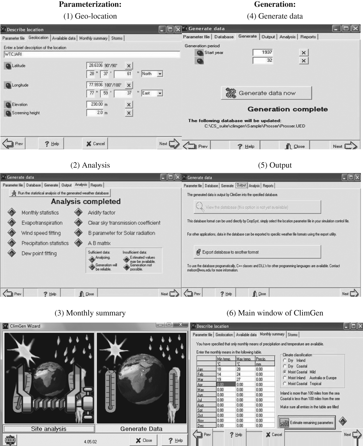
In the present study, the ClimGen model was parameterized using 37 years (1972–2008) of daily weather records comprising rainfall, minimum and maximum air temperatures, relative humidity, wind speed, rainfall and sunshine time for the IARI farm (28°32′N, 78°17′E, altitude 167·5 m). Screenshots from ClimGen during the data parameterization and generation process are shown in Fig. 1.

Fig. 1. Captured window of ClimGen model for different activities of data parameterization and generation.
Use of CROPWAT to estimate irrigation scheduling
Computer programs dealing with computations of crop water requirements are mainly based on a reference evapotranspiration. These programs have either a single purpose, to estimate crop water requirement, or are embedded as a module of CROPWAT 8.0 (FAO 2009). CROPWAT is used widely by researchers for estimation of evapotranspiration, crop water requirements and irrigation scheduling of different crops. CROPWAT ver 8.0 employs the Modified Penman–Monteith (PENMON) approach in estimating evapotranspiration. It is tested extensively, widely accepted and also recommended by the FAO (Lenselink & Jurriens Reference Lenselink and Jurriens1993). The model also calculates the percentage reduction in crop yield due to water stress during the cropping period. The program algorithm allows development of irrigation schedules for different management conditions and calculation of water supply under varying cropping patterns.
AquaCrop model description
In this context, the recently developed FAO AquaCrop model (Raes et al. Reference Raes, Steduto, Hsiao and Fereres2009; Steduto et al. Reference Steduto, Hsiao, Raes and Fereres2009) is a user-friendly and practitioner-oriented model because it maintains an optimal balance between accuracy, robustness and simplicity, and requires a relatively small number of model input parameters. AquaCrop has been parameterized and tested on maize by using experimental data from six cropping seasons at the University of California, Davis, USA (Hsiao et al. Reference Hsiao, Heng, Steduto, Rojas-Lara, Raes and Fereres2009). Hsiao et al. (Reference Hsiao, Heng, Steduto, Rojas-Lara, Raes and Fereres2009) observed that AquaCrop was able to simulate the canopy cover, biomass development and grain yield of four maize cultivars over six different cropping seasons that differed in plant density, planting date and evaporative demands. Araya et al. (Reference Araya, Habtu, Hadgu, Kebede and Dejene2010) evaluated the AquaCrop model for simulating biomass and yield of water deficient and irrigated barley in Northern Ethiopia and reported that the AquaCrop model performed well, with model efficiency ranging from 0·5 to 0·95 for grain yield under various planting dates. Stricevic et al. (Reference Stricevic, Cosic, Djurovic, Pejic and Maksimovic2011) evaluated the AquaCrop model in Serbia for maize, sugar beet and sunflower under rainfed conditions or provided with supplementary irrigation: they reported that the maximum prediction error for maize was 3·6% and for sugar beet 12·2%. However, they concluded that the AquaCrop model can be used in impartial decision-making and in the selection of crops to be given irrigation priority in areas where water resources are limited.
Input data requirement of AquaCrop model
Operation of the AquaCrop model requires input data consisting of climatic parameters and management data for the crop, soil, field and irrigation. However, the model contains a complete set of input parameters that can be selected and adjusted for different soil or crop types.
Climate data
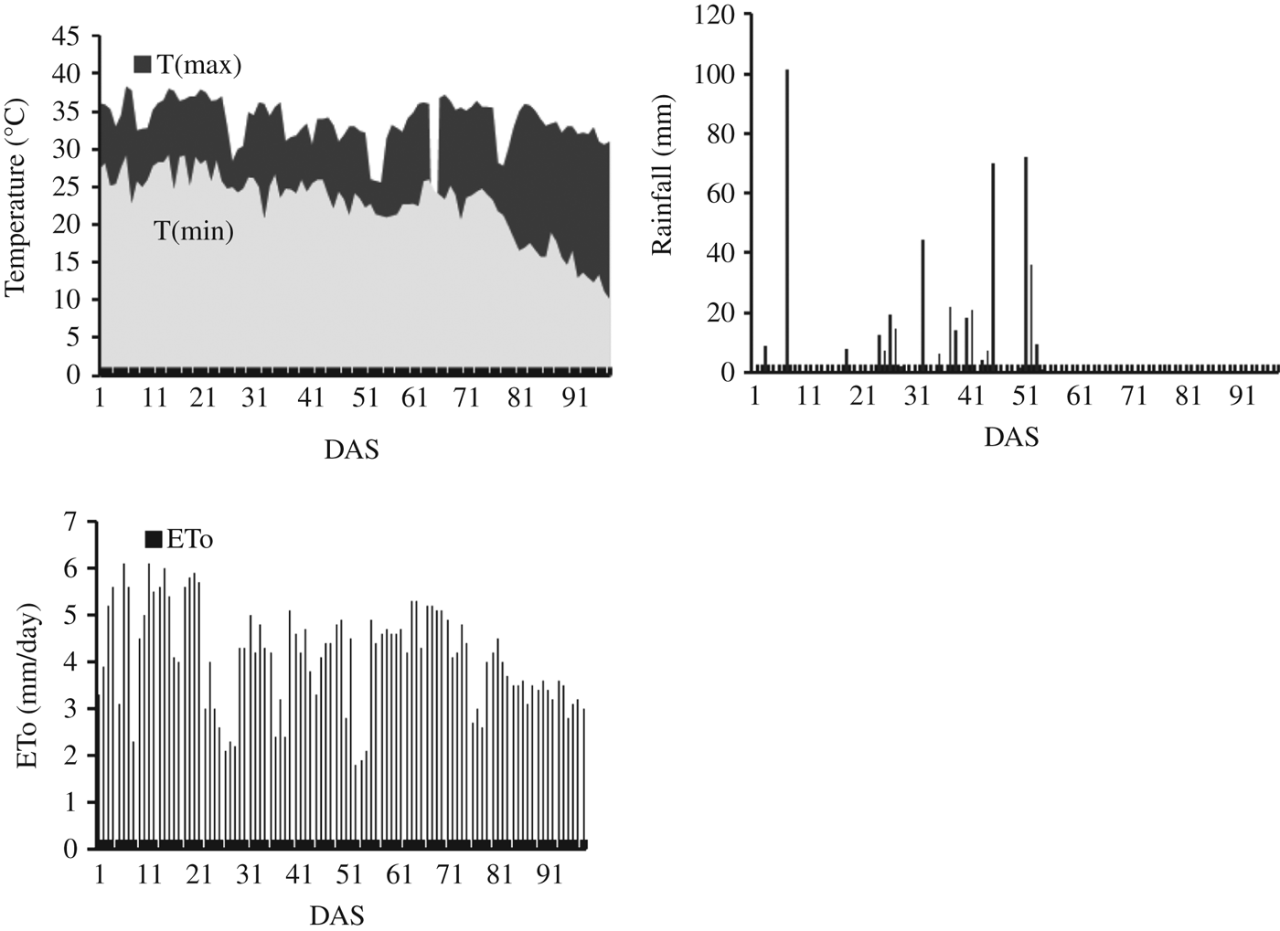
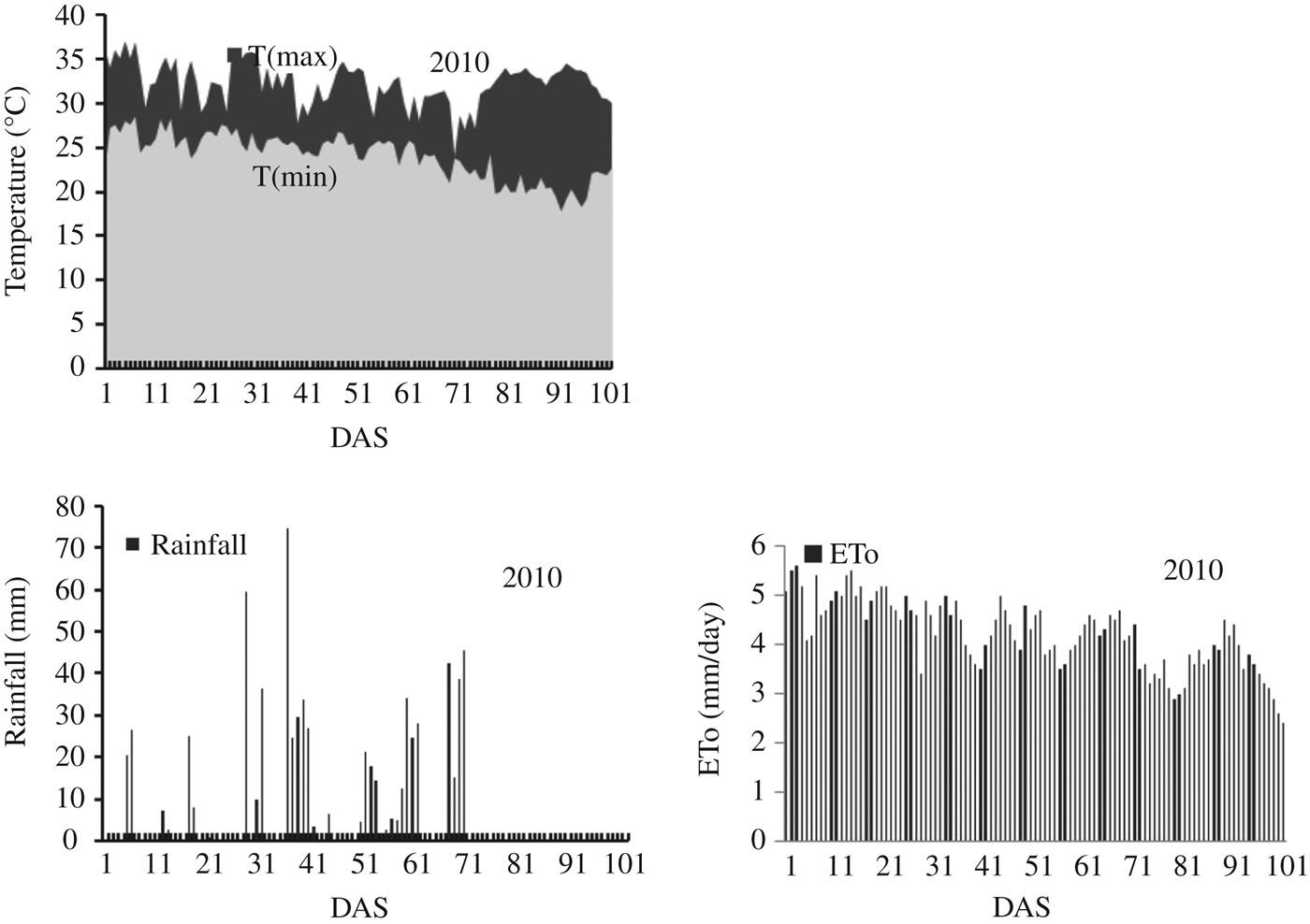
The weather data required by AquaCrop are daily values of minimum and maximum air temperature, ETo, rainfall and mean annual carbon dioxide (CO2) concentration. The ETo was estimated with an ETo calculator using the daily maximum and minimum temperature, wind speed at 2 m above ground surface, solar radiation and mean relative humidity. The weather parameters were collected from an automatic weather station located at a distance of 150 m from the WTC-01 experimental farm. Rainfall of 502 and 713 mm during the growing season were recorded in 2009 and 2010, respectively. The temperature variations, ETo and rainfall during the crop-growing period of 2009 and 2010 are shown in Figs 2 and 3, respectively.

Fig. 2 Weather parameters during the crop growth period in days after sowing (DAS) for the year 2009.

Fig. 3 Weather parameters during the crop growth period in days after sowing (DAS) for the year 2010.
Crop parameters
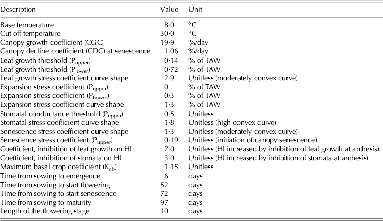
Canopy development was measured once in every 2 weeks by removing two plants per plot and recording growth stage, leaf area, root length and above-ground biomass. Date of emergence, maximum canopy cover, duration of flowering, start of senescence and maturity were also recorded. At each crop growth stage, green leaves were separated and the leaf area of each plant measured using a leaf area meter (LI-3100C by LI-COR Inc., USA) to obtain the leaf area index (LAI), which was converted to crop canopy cover for use as input data for AquaCrop model simulation. Dry weight of above-ground biomass at each growth stage was obtained after oven drying for 48 h at 65 °C. Other measurements were taken from Hsiao et al. (Reference Hsiao, Heng, Steduto, Rojas-Lara, Raes and Fereres2009): the canopy decline coefficient, crop coefficient for transpiration at full canopy cover, soil water depletion thresholds for inhibition of leaf growth and stomatal conductance and acceleration of canopy senescence. These parameters were presumed to be applicable to a wide range of conditions and not specific to a given crop cultivar. The full range of crop parameters used as input to AquaCrop is presented in Table 2. The relationship between LAI and canopy cover used for maize crop was calculated using Eqn (1) (Hsiao et al. Reference Hsiao, Heng, Steduto, Rojas-Lara, Raes and Fereres2009):
Table 2. Input data of crop parameters used in AquaCrop model

TAW: total available water.
The upper and lower thresholds and the shape of the response curve are the parameters for each type of stress that define the sensitivity and severity of a depleted soil profile. The upper threshold determines when the stress begins, whereas the lower threshold is the point at which the physiological process ceases completely. The shape factor used in AquaCrop describes the amplitude of the stresses, which affect crop yield. A shape factor of zero indicates the highest sensitivity of a crop to water stress while values >0 are indicative of a lower sensitivity to water stress. The water stress is divided into expansion stress, stomatal closure stress and senescence stress coefficients. These coefficients were calibrated using the experimental data to obtain a better match between AquaCrop simulated and observed data.
Soil parameters
Data pertaining to the soil at the experimental site, required as input parameters for AquaCrop, are: number of soil horizons, soil texture, field capacity, permanent wilting point, saturated hydraulic conductivity and volumetric water content at saturation. The experimental site did not contain any impervious or restrictive soil layer to obstruct the expansion of root growth. The curve number of the site was used to estimate surface runoff from rainfall that occurred during the experiment.
Irrigation and field management parameters
Irrigation and field management during the experiment are two important components considered in the AquaCrop model. Irrigation management comprised data pertaining to both rainfed (no irrigation) and irrigation conditions. In the full irrigation treatment (W4), water was applied up to field capacity when soil moisture in the root zone approached 50% of total available water. In the deficit irrigation treatments (i.e. 50 and 75% of full irrigation, designated W2 and W3, respectively), water was applied on the same day as the fully irrigated plot, but the irrigation depths were reduced to 50 and 75% of the full irrigation. There was no irrigation (W1) in the rainfed plots. The field management components were fertility levels (i.e. no nitrogen (N1), 75 kg N/ha (N2) and recommended or full fertilization of 150 kg N/ha (N3)), mulching to reduce evaporation from the soil and furrow end bunds to eliminate surface runoff. In the present study, the AquaCrop model was evaluated through calibration and validation to estimate yield, biomass and canopy cover under the different water and nitrogen levels detailed above.
Operation of ClimGen, CROPWAT and AquaCrop to generate future maize yield
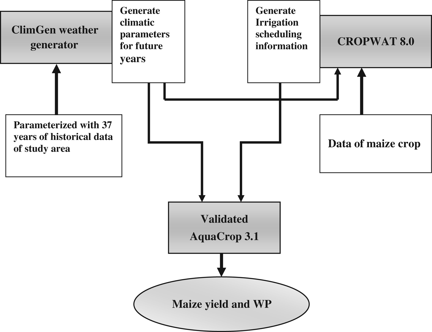
The data obtained from ClimGen were used in the CROPWAT model to determine irrigation scheduling for a maize crop in the kharif season of years 2011, 2012, 2013 and 2014. Schematic architecture of linking different models to generate future yield of maize under variable water availability scenarios is presented in Fig. 4. The CROPWAT was used to estimate the date and depth of irrigation, a facility that is not available in AquaCrop. The generated climate data of these 4 years and the irrigation scheduling information was used in the validated AquaCrop model to predict maize grain yield, biomass and water productivity (the ratio of grain yield to the amount of total water used (i.e. sum of irrigation and the effective rainfall during the crop growth period)). In addition, the best sowing date to obtain maximum yield was also generated by simulation using the AquaCrop model. The validated AquaCrop model was used for generation of future scenarios. The yield variations under different irrigation water and nitrogen levels were also obtained by simulation through the AquaCrop model (Table 3). The inputs to the model for different years were the climatic data, date and depth of irrigation and varying nitrogen levels. The soil and crop parameters were kept the same as that used in the model validation for the year 2010. A similar approach could be replicated to other future years using the generated climate data and the model linking protocols to obtain the future maize yield.

Fig. 4. Schematic architecture of linking different models to generate future yield of maize under variable water availability scenarios.
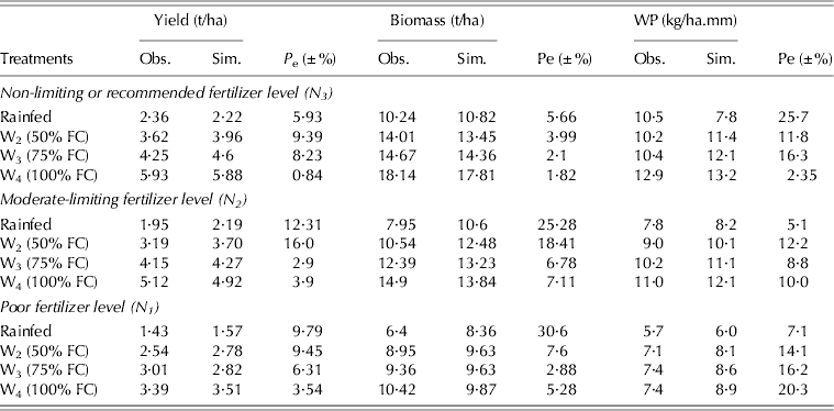
Table 3. Calibration results of biomass, grain yield and water productivity (WP) of maize under different irrigation water and fertilizer regimes

Obs., observed; Sim., simulated; Pe, prediction error.
RESULTS AND DISCUSSION
AquaCrop model calibration results
The AquaCrop model was calibrated using the experimental data from 2009 to predict canopy cover, grain yield and biomass under different water and fertilizer application levels in the experiment. The calibrated and observed data for biomass, grain yield and water productivity in all treatment combinations are presented in Table 3 and the results of grain yield are plotted in Fig. 5.

Fig. 5. Model calibration results for grain yield under different irrigation and nitrogen levels. E, model efficiency; MAE, mean absolute error.
The results of model performance pertaining to grain yield are shown in Fig. 5. The maximum and minimum errors in grain yield prediction were observed in the W2N2 and W4N3 treatments, amounting to 16 and 0·84%, respectively (Table 3). The model was calibrated for grain yield with the Nash-Sutcliffe model efficiency E (Nash & Sutcliffe Reference Nash and Sutcliffe1970) and R 2 of 0·99, respectively. The prediction error in biomass for W1N1 and W4N3 treatments were 30·6 and 1·82%, respectively (Table 3). The best calibrated AquaCrop model was obtained with prediction error ranging from a minimum of 0·07% for the full irrigation treatment (W4) to a maximum of 4·1% in W2 (50% FC) for all nitrogen levels. Similarly, the highest (13·4%) and the lowest prediction error (2·5%) for biomass were in rainfed crops and in the W3 treatment (i.e. 75% FC), respectively, at all the nitrogen levels. The best calibrated AquaCrop model for water productivity was obtained with prediction error ranging from the maximum of 27·5% in the W1N3 treatment to the minimum of 2·35% in the W4N3 treatment, respectively (Table 3). The prediction error statistics of the calibrated model are presented in Table 4. The model was calibrated for simulation of yield and biomass for all treatment levels with the prediction error statistics of model efficiency (E) (0·95<E<0·99) root-mean-square error (RMSE) (0·29<RMSE<0·42) and mean absolute error (MAE) (0·17<MAE<0·51 t/ha). AquaCrop model predictions for grain yield and biomass were in line with the observed data which were corroborated with E and R 2 values approaching one. However, the water productivity during calibration was with E of 0·66 and R 2 of 0·8 (Table 4). The model calibration results and the observed values of grain yield, for all treatment combinations are plotted in Fig. 5.
Table 4. Prediction error statistics of the calibrated AquaCrop model

AquaCrop model validation results
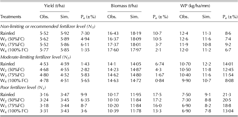
It was observed that the maximum and minimum errors of grain yield prediction during model validation with the data of 2010 were for the W1N1 and W4N3 treatments, amounting to 9·9 and 1·35% respectively (Table 5). Morever, the maximum and minimum errors for biomass were obserevd to be in the W1N1 and W4N2 treatments (17·5 and 0·48%, respectively) (Table 5). The AquaCrop model was validated with the prediction error ranging from a minimum of 0·47% for the full irrigation treatment (W4) to a maximum of 5·91% in rainfed (W1) under all nitrogen levels. Similarly, the highest (11·06%) and the lowest prediction error (4·36%) for biomass were observed for rainfed conditions and in (W4) treatment (i.e. 100% FC), respectively (Table 5). The prediction error statistics of model validation are shown in Table 6. It can be observed from Table 6 that the model was validated for yield and biomass with all treatment combinations for the prediction error statistics parameters viz. E, RMSE, R 2 and MAE varying from 0·95<E<0·98, 0·1<RMSE<0·75, 0·9<R 2<0·96 and 0·11<MAE<1·08 t/ha. Moreover, the model was validated for simulating the water productivity for all irrigation levels with the prediction error statistics E and R 2 values of 0·74 and 0·77, respectively. The model validation results and the observed values of grain yield for all treatment combinations were plotted (Fig. 6). It can be seen from Fig. 6 that the E and R 2 values for grain yield and biomass predictions by the AquaCrop model under different irrigation water and nitrogen regimes were in line with the observed values.

Fig. 6. Model validation results in simulating grain yield of maize under different irrigation and nitrogen levels. E, model efficiency; MAE, mean absolute error.
Table 5. Validation results of biomass and grain yield of maize under different irrigation water and nitrogen regimes

Table 6. Prediction error statistics of the validated AquaCrop model

Linking of models results
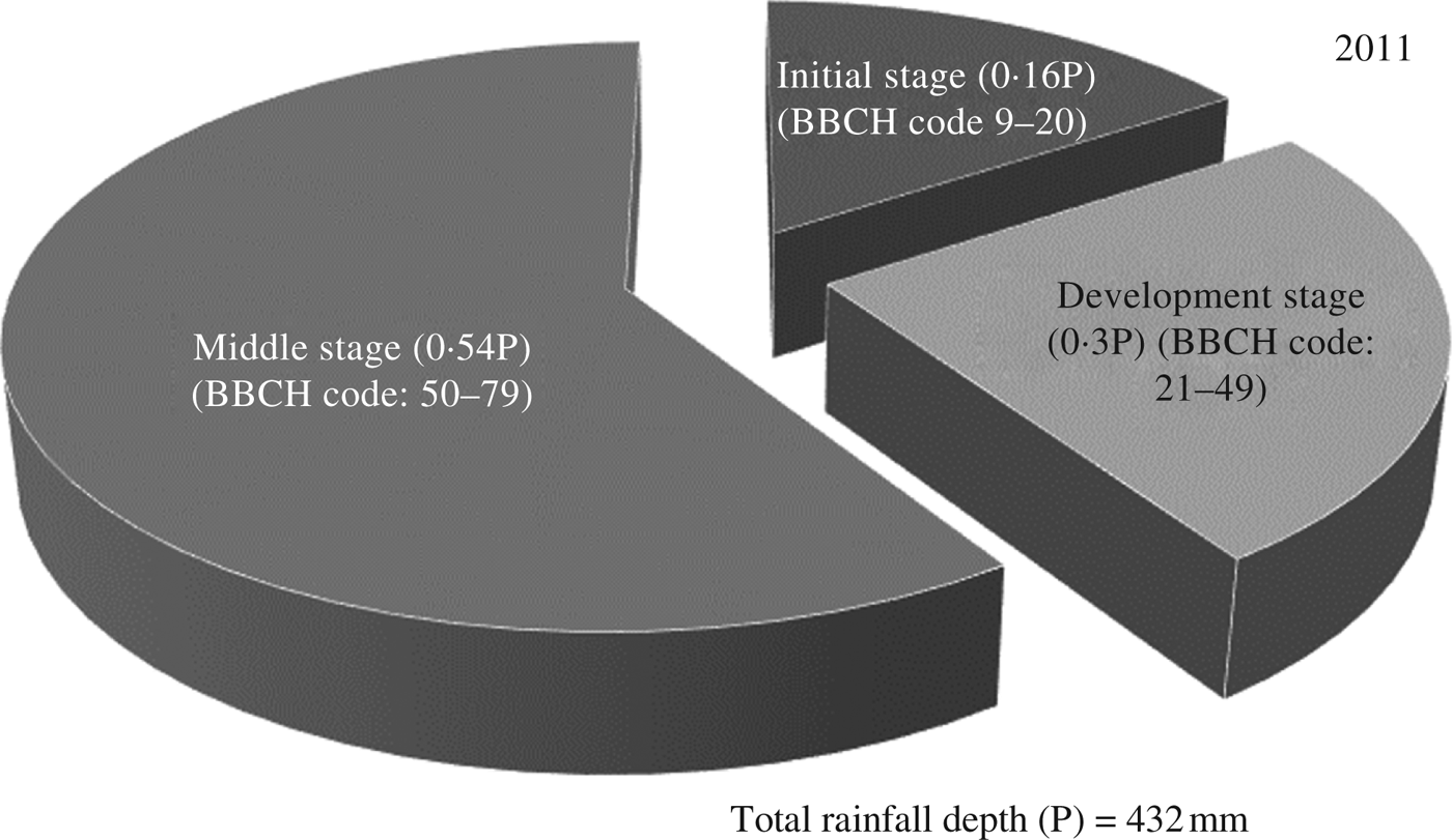
ClimGen-generated rainfall depth during the growing seasons of 2011, 2012, 2013 and 2014 are shown in Tables 7–10, respectively. The total rainfall was 432 mm during the maize-growing season in 2011 (Table 7) and the proportions occurring during four different maize growth stages, termed here as initial (corresponding to BBCH code: 9–20; Lancashire et al. Reference Lancashire, Bleiholder, Langeluddecke, Stauss, van den Boom, Weber and Witzen-Berger1991), development (BBCH code: 21–49), middle (BBCH code: 50–9) and late stages (BBCH code: 80–99) were 0·16, 0·25, 0·59 and 0·00 of total rainfall, respectively (Fig. 7). It can also be seen that, as per the ClimGen-generated data, there was no rainfall for 58 days after sowing (DAS) the crop on 22 July. Therefore, irrigation will be necessary at this sensitive crop growth stage to reduce the effect of water stress. Under these scenarios, application of three irrigations of 51 mm each at 42, 72 and 92 DAS, amounting to a total irrigation depth of 153 mm, was predicted for 2011 using the CROPWAT model. Furthermore, using the information generated for climate, irrigation scheduling, soil and crop data, maize yield as simulated by AquaCrop varied from 3400 to 5900 kg/ha under different irrigation and nitrogen levels (Table 7). Also, under the rainfed scenarios with recommended nitrogen dose (W1N3), the maize yield was 3490 kg/ha.

Fig. 7. Distribution of rainfall (P) during different crop growth stages (sowing date: 22 July 2011).
Table 7. Predicted rainfall distribution, irrigation scheduling and yield of maize under different treatments during 2011

Total rainfall (P) during the crop-growing season, 432 mm. Total depth of irrigation, 153 mm.
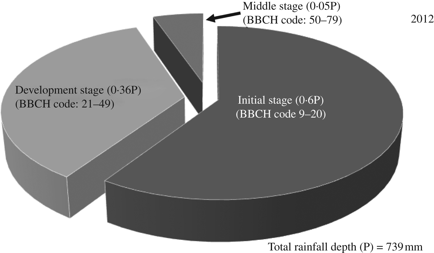
Similarly for the year 2012, the total rainfall depth predicted by ClimGen was 739 mm and the irrigation scheduling estimated by CROPWAT was 51 DAS and 56 mm (Table 8). The proportions of rainfall depth during the initial (BBCH code: 9–20), development (BBCH code: 21–49), middle (BBCH code: 50–79) and late (BBCH code: 80–99) maize growth stages were 0·59, 0·36, 0·05 and 0·00 of total rainfall, respectively (Fig. 8). Subsequently, the AquaCrop model prediction for maize grain yield was 5920 kg/ha under full irrigation (W4) and 1600 kg/ha under the rainfed scenario (W1) with recommended nitrogen dose (N3). The predicted grain yield under rainfed conditions for 2012 was less than that of 2011, which may be attributed to less rainfall in 2012 during the grain formation stage.

Fig. 8. Distribution of rainfall (P) during different crop growth stages (sowing date: 22 July 2012).
Table 8. Predicted rainfall distribution, irrigation scheduling and yield of maize under different treatments during 2012

Total rainfall (P) during the crop-growing season, 739 mm. Total depth of irrigation, 56 mm.
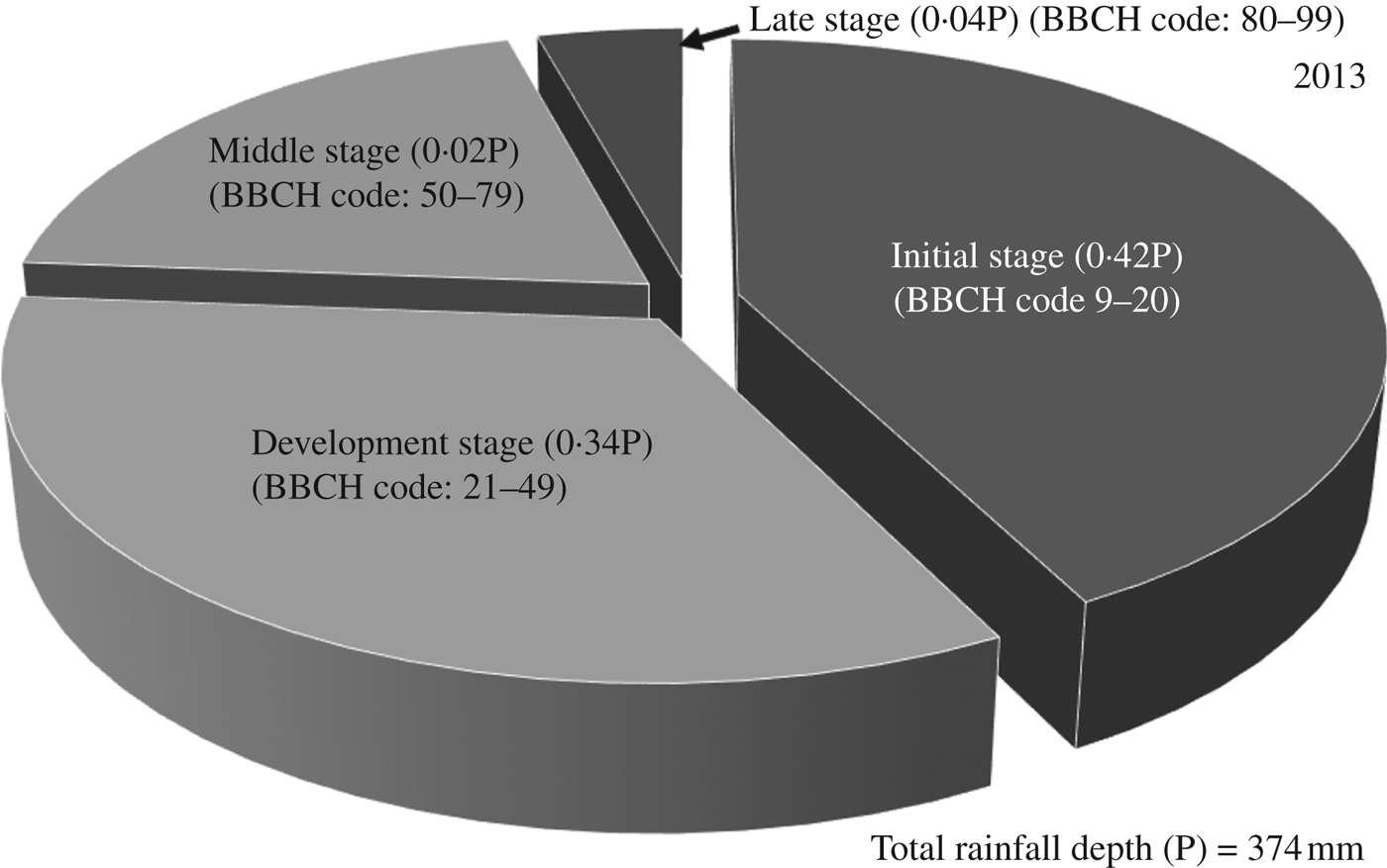
For 2013, the ClimGen-generated rainfall depth during the maize growing period was 374 mm (Table 9), with proportions of rain falling during the four growth stages of 0·42, 0·34, 0·20 and 0·04 of total rainfall, respectively (Fig. 9). Therefore, three irrigation requirements of 59, 68 and 64 mm at 47, 66, 75 DAS, amounting to a total irrigation depth of 191 mm, was generated for the year 2013 by the CROPWAT model. Using these parameters, AquaCrop predicted a maize grain yield of 5900 kg/ha under full irrigation (W4), while under the rainfed scenarios (W1) with recommended nitrogen dose (N3), the maize yield was 1400 kg/ha. The highest maize grain yield was predicted to be 5900 kg/ha in the year 2013 with full irrigation and recommended dose of N fertilizer (N3), with rainfall of 374 mm during the crop-growing period coupled with four irrigations totalling 191 mm (Fig. 9). However, the predicted maize yield for 2012 with higher than normal rainfall depth of 739 mm and with two irrigations of 113 mm was 5920 kg/ha. In contrast, the higher than normal rainfall depths generated for 2012 (739 mm) and 2014 (625 mm) resulted in grain yield of 1600 and 5670 kg/ha, respectively, under rainfed conditions with a full dose of fertilizer (N3). This difference in yield may be attributed to the occurrence of rainfall during the sensitive growth stages (BBCH codes: 51–71) after the sowing date of 22 July in both these years (Tables 8 and 10).

Fig. 9. Distribution of rainfall (P) during different crop growth stages (sowing date: 22 July 2013).
Table 9. Predicted rainfall distribution, irrigation scheduling and yield of maize under different treatments during 2013

Total rainfall during the crop-growing season, 374 mm. Total depth of irrigation, 191 mm.
Table 10. Predicted rainfall distribution, irrigation scheduling and yield of maize under different treatments during 2014

Total rainfall during the crop-growing season, 625 mm. Total depth of irrigation, 52 mm.
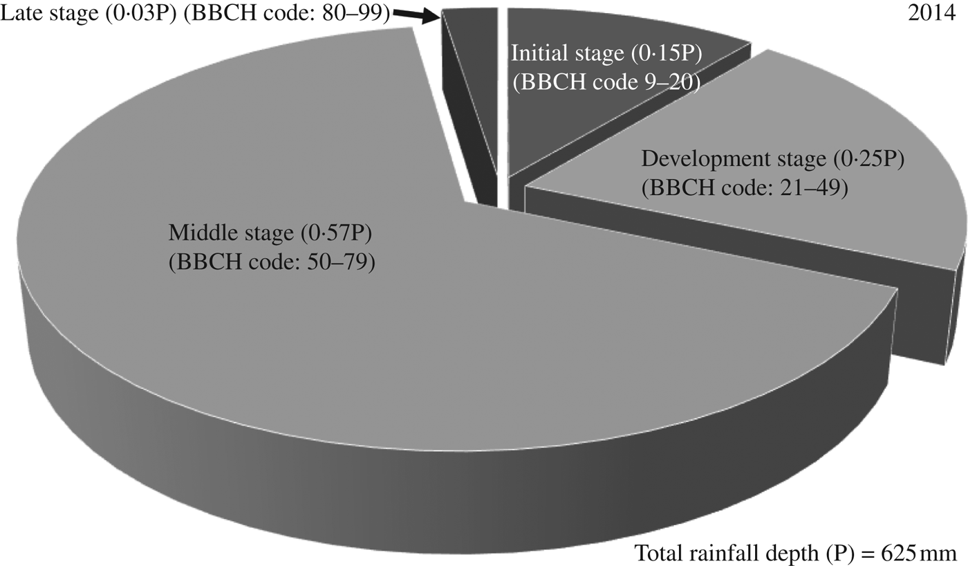
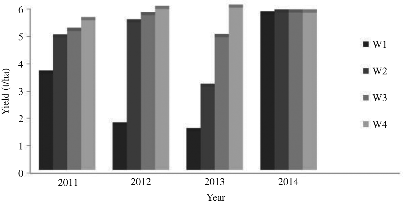
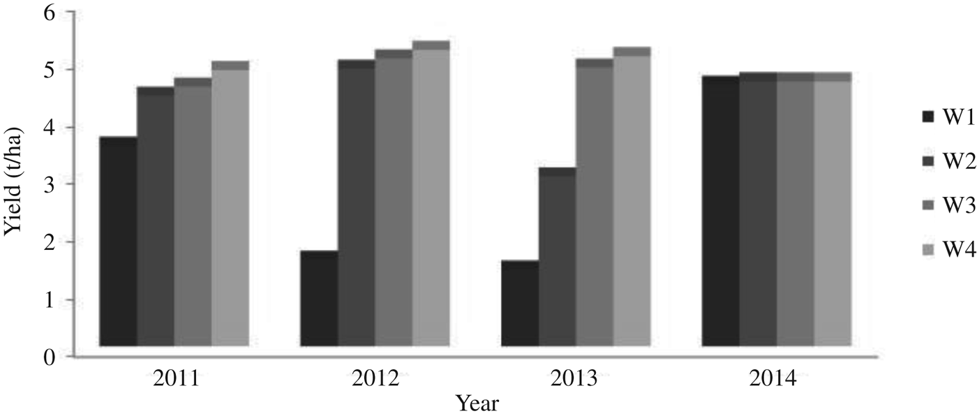
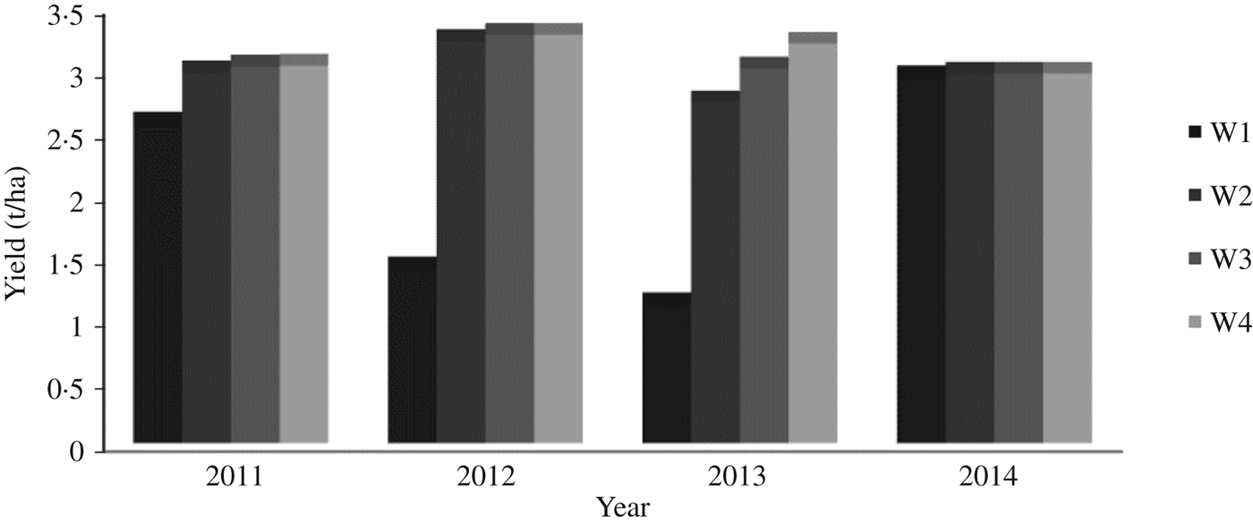
Similarly for 2014, the total rainfall depth predicted by ClimGen was 625 mm and the irrigation schedule generated by CROPWAT was 64 DAS and 52 mm (Table 10). The proportions of rainfall during the initial (BBCH code: 9–20), development (BBCH code: 21–49), middle (BBCH code: 50–79) and late stages (BBCH code: 80–99) of maize growth were 0·15, 0·25, 0·57 and 0·03 of total rainfall, respectively (Fig. 10). AquaCrop predicted maize grain yield of 5800 kg/ha under full irrigation with recommended nitrogen dose N3. Also, under rainfed conditions with recommended nitrogen dose (W1N3), the maize yield was 5670 kg/ha. Maize grain yield predictions under different irrigation and nitrogen levels for 4 years from 2011 to 2014 are shown in Figs 11to13, respectively, for 150 (N3), 75 (N2) and 0 (N1) kg N/ha nitrogen levels. It can be observed from these figures that there was minimal difference in yield for different irrigation water treatments during the year 2014 and the trend was the same for all N fertilization levels. This may be attributed to occurrence of well distributed and above-normal rainfall depth of 625 mm during the crop-growing period of 2014. Also, there was one irrigation of 52 mm at 64 DAS during the year 2014 (Table 10). Therefore, the model-predicted data showed that there was no effect of irrigation on crop yield during the year 2014.

Fig. 10. Distribution of rainfall (P) during different crop growth stages (sowing date: 22 July 2014).

Fig. 11. Prediction of maize yield with non-limited fertilizer (N3) under different irrigation levels.

Fig. 12. Prediction of maize yield with moderate fertilizer (N2) under different irrigation levels.

Fig. 13. Prediction of maize yield under poor fertilizer (N1) and varying irrigation levels.
CONCLUSIONS
Judicious selection of models pertaining to climate generation, irrigation scheduling and crop growth and their meticulous use plays a vital role in prediction of crop yield under future water availability scenarios. In the present study, ClimGen, CROPWAT and validated AquaCrop models were linked to predict future maize yield under different irrigation and N-fertilization levels. It was observed that the sowing date of the crop would play a significant role in obtaining maximum yield under the ClimGen generated future rainfall distributions. The AquaCrop model predicted data for four future years and revealed significant yield variations of kharif maize with different water and nitrogen supply situations under deficit irrigation. It was also observed that bringing forward the sowing date, as obtained from model predictions, to 1st July 2012 would result in better yield under rainfed conditions. Therefore, linkage of ClimGen, CROPWAT and AquaCrop can assist in prediction of sowing date, irrigation scheduling and crop growth/yield parameters under changing climate scenarios. Moreover, the model-linking protocol developed in the present study can be replicated over different locations after successful calibration of the models. In addition, the predictions of rainfall, irrigation depths and crop yield need to be ascertained with the observed data of future years to judge its accuracy and wide applicability.
The authors wish to acknowledge the financial assistance provided under a sub-project of National Agricultural Innovation Project (NAIP), Indian Council of Agricultural Research (ICAR) to undertake the research work at Water Technology Centre, IARI, New Delhi, India.

