


1. Introduction
The mathematical analysis of the robustness of random graphs and networks has been the focus of research interest in the last two decades [Reference Albert, Jeong and Barabási1, Reference Callaway5, Reference Li18, Reference Shao28]. The robustness of a network refers to its ability to maintain the overall connectivity against random error or targeted attack, i.e., how its structure varies when a fraction of its vertices or edges are removed. This question can be investigated using the tools of an established field of statistical physics called percolation theory.
Most of the works have focused on classical percolation on networks, meaning that each vertex (site) or edge (bond) is kept (occupied) with probability p and removed (vacant) with probability $1-p$
; see, e.g., [Reference Li18]. This way of keeping or removing edges models how the network performs under random failures. One fundamental question is whether there is a giant connected component of macroscopic size in the remaining graph. Percolation theory studies the emergence of such a component when we increase the probability p. Usually there is a well-defined critical point
$1-p$
; see, e.g., [Reference Li18]. This way of keeping or removing edges models how the network performs under random failures. One fundamental question is whether there is a giant connected component of macroscopic size in the remaining graph. Percolation theory studies the emergence of such a component when we increase the probability p. Usually there is a well-defined critical point $p_\textrm{c}$
above which there exists a unique giant component. This critical point is also called the percolation threshold and this phenomenon is referred to as percolation phase transition.
$p_\textrm{c}$
above which there exists a unique giant component. This critical point is also called the percolation threshold and this phenomenon is referred to as percolation phase transition.
Besides classical network percolation, another well-studied model is when the vertices or edges are removed with preference, for example the nodes can be targeted preferentially according to a structural property such as the degree or betweenness centrality. Scale-free networks were found to be robust under random failures, and extremely vulnerable to targeted attacks [Reference Albert, Jeong and Barabási1].
Several other network percolation frameworks have been proposed in the literature over the years, including k-core percolation [Reference Dorogovtsev, Goltsev and Mendes7], bootstrap percolation [Reference Baxter4], l-hop percolation [Reference Shang, Luo and Xu27], and limited path percolation [Reference López21]. For an extensive review on network percolation, see [Reference Li18].
In this paper, we focus on another recent network percolation framework called color-avoiding percolation [Reference Kadović13, Reference Krause, Danziger and Zlatić15, Reference Krause, Danziger and Zlatić16]. In this framework, each vertex or edge is assigned a color from a color set; a color may represent a shared eavesdropper, a controlling entity, or a correlated failure. Two vertices are color-avoiding connected if they can be reached from each other on paths that avoid any color from the color set. Therefore, while in the traditional percolation framework a single path provides connectivity, here connectivity refers to the ability to avoid all vulnerable sets of vertices or edges. The main rationale behind this percolation model is that in real-world networks some nodes or links may mutually share a vulnerability and it is interesting to see whether the network is robustly connected in the sense that its overall connectivity is maintained in every possible attack scenario.
The color-avoiding percolation framework differs substantially from k-core percolation, where any k paths are sufficient between two nodes in the percolating cluster [Reference Dorogovtsev, Goltsev and Mendes7, Reference Yuan33], and it is also different from k-connectivity, where k pairwise disjoint paths are required [Reference Penrose25]. Another relevant framework is percolation on multiplex networks [Reference Hackett11, Reference Mahabadi, Varga and Dolan23, Reference Son30], where the layers can be considered as colors. However, this approach also differs in the definition of connectivity as discussed in detail in [Reference Krause, Danziger and Zlatić15]. Percolation on colored networks was also investigated in [Reference Kryven17]; however, in that setup, colors do not indicate shared vulnerabilities, but the removal probability depends on the color.
Networks with colored vertices were also investigated in [Reference Krause, Danziger and Zlatić15], which not only presented a heuristic analytical framework for the configuration model together with a numerical algorithm to determine the color-avoiding connected pairs of nodes, but also demonstrated the applicability of the color-avoiding percolation in cybersecurity. It extended the theory of color-avoiding site percolation by studying the phase transition for Erdős–Rényi random graphs and by introducing novel node functions to generalize the concept [Reference Krause, Danziger and Zlatić16]. This framework was further developed to study secure message-passing in networks with a given community structure [Reference Shekhtman29]. Color-avoiding percolation in diluted lattices was investigated in [Reference Giusfredi and Bagnoli10], and in [Reference Giusfredi and Bagnoli9] it was shown that color-avoiding site percolation can be mapped into a self-organized critical problem.
In [Reference Kadović13], (not necessarily properly) edge-colored networks were studied, and both analytical and numerical results presented concerning the size of the giant color-avoiding connected component for Erdős–Rényi and for scale-free graphs.
A similar concept called ‘courteous edge-coloring’ was studied in [Reference DeVos, Johnson and Seymour6]. Graphs with 1-courteous edge-colorings are exactly the edge-color-avoiding connected graphs. That article gave interesting upper bounds on the number of colors needed to courteously color an arbitrary graph.
The computational complexity of finding the color-avoiding connected components in both vertex- and edge-colored setups was investigated in [Reference Molontay and Varga24], and it was found that the complexity of color-avoiding site percolation highly depends on the exact formulation: a strong version of the problem is NP-hard, while a weaker notion makes it possible to find the components in polynomial time. However, in the bond percolation setup, the color-avoiding connected components can be found in polynomial time.
The goal of this paper is to study some key observables associated with the color-avoiding bond percolation setup on Erdős–Rényi random graphs. We explicitly calculate the empirical density of the giant color-avoiding connected component (if it exists) with an arbitrary number of randomly distributed colors. Moreover, we also give an explicit formula for the empirical density of the sizes of color-avoiding connected components in the case of two-colored Erdős–Rényi random graphs. The methods we apply are classical (e.g. local approximation of random graphs by Galton–Watson trees, method of generating functions), but the analysis is more involved.
A few months after we posted an earlier, longer version [Reference Ráth26] of this paper on arXiv, a new paper [Reference Lichev and Schapira20] on color-avoiding percolation on edge-colored Erdős–Rényi graphs also appeared. The results of [Reference Lichev and Schapira20] include simplification and generalization of some of our results in [Reference Ráth26] and the answers to some of the open questions that we posed, as well as some finer results on the size of the largest color-avoiding component; see Section 2.2 for more details. It also described the phase transition of the largest color-avoiding connected component between the supercritical and the intermediate regime [Reference Lichev19]. Our current paper only contains results that are already stated and proved in [Reference Ráth26], but we have removed the proofs of those results concerning the convergence of the color-avoiding component structure of edge-colored Erdős–Rényi graphs that are also proved in [Reference Lichev and Schapira20].
The paper is organized as follows. In Section 2, we collect the basic definitions needed for this paper, state our main results, and then recall some key results from [Reference Lichev and Schapira20, Reference Ráth26] that help to put our main results in context. In Section 3, we introduce some further notation and we prove some preliminary results about the survival of certain edge-colored branching processes. In Section 4, we give formulas for the asymptotic size of the giant color-avoiding connected component (if it exists) and we also study its barely supercritical behavior. In Section 5, we give a formula for the distribution of the sizes of the small components when there are only two colors. Finally, in Section 6, we propose some open questions.
2. Main results and their context
We denote the sets of real, positive real, nonnegative integer, and positive integer numbers by $\mathbb{R}$
,
$\mathbb{R}$
, $\mathbb{R}_+$
,
$\mathbb{R}_+$
, $\mathbb{N}$
, and
$\mathbb{N}$
, and $\mathbb{N}_+$
, respectively, and we use the notation
$\mathbb{N}_+$
, respectively, and we use the notation $[n] = \{1, 2, \ldots, n \}$
for any
$[n] = \{1, 2, \ldots, n \}$
for any $n \in \mathbb{N}_+$
. If A is an event, we denote by
$n \in \mathbb{N}_+$
. If A is an event, we denote by $\textbf{1}[A]$
the indicator variable of the event:
$\textbf{1}[A]$
the indicator variable of the event: $\textbf{1}[A] = 1$
if A occurs, and
$\textbf{1}[A] = 1$
if A occurs, and $\textbf{1}[A] = 0$
if the complement of A, i.e.
$\textbf{1}[A] = 0$
if the complement of A, i.e. $A^\textrm{c}$
, occurs. Throughout the article, by edge-colorings we always mean not necessarily proper ones and by paths we always mean simple paths (and not walks).
$A^\textrm{c}$
, occurs. Throughout the article, by edge-colorings we always mean not necessarily proper ones and by paths we always mean simple paths (and not walks).
Definition 2.1. (Edge-colored (multi)graph.) We say that $G=(V,\underline{E})$
is an edge-colored (multi)graph with
$G=(V,\underline{E})$
is an edge-colored (multi)graph with $k \in \mathbb{N}_+$
colors if
$k \in \mathbb{N}_+$
colors if $\underline{E} = (E_1, \ldots, E_k)$
and
$\underline{E} = (E_1, \ldots, E_k)$
and $E_i \subseteq \binom{V}{2}$
for every
$E_i \subseteq \binom{V}{2}$
for every $i \in [k]$
. We say that V is the vertex set of G and
$i \in [k]$
. We say that V is the vertex set of G and $E_i$
is the set of edges of color i for every
$E_i$
is the set of edges of color i for every $i \in [k]$
.
$i \in [k]$
.
Note that the edge sets $E_1, \ldots, E_k$
are not necessarily disjoint, and the edges of
$E_1, \ldots, E_k$
are not necessarily disjoint, and the edges of $E_i$
are not necessarily independent in the graph-theoretical sense for any
$E_i$
are not necessarily independent in the graph-theoretical sense for any $i \in [k]$
(i.e. the graph G is not necessarily properly edge-colored).
$i \in [k]$
(i.e. the graph G is not necessarily properly edge-colored).
Definition 2.2. (Uncolored color-subgraphs.) Given an edge-colored graph $G = (V, \underline{E})$
with
$G = (V, \underline{E})$
with $k \in \mathbb{N}_+$
colors, where
$k \in \mathbb{N}_+$
colors, where $\underline{E} = (E_1, \ldots, E_k)$
, let
$\underline{E} = (E_1, \ldots, E_k)$
, let $G^I$
denote the simple uncolored graph
$G^I$
denote the simple uncolored graph $\big( V, \bigcup_{i \in I} E_i \big)$
. In addition, we write
$\big( V, \bigcup_{i \in I} E_i \big)$
. In addition, we write $G^{\textrm{uc}} \,:\!=\, G^{[k]}$
and
$G^{\textrm{uc}} \,:\!=\, G^{[k]}$
and $G^{\setminus i} \,:\!=\, G^{[k] \setminus \{ i \}}$
for any
$G^{\setminus i} \,:\!=\, G^{[k] \setminus \{ i \}}$
for any $i \in [k]$
.
$i \in [k]$
.
For an example, see Figure 1.
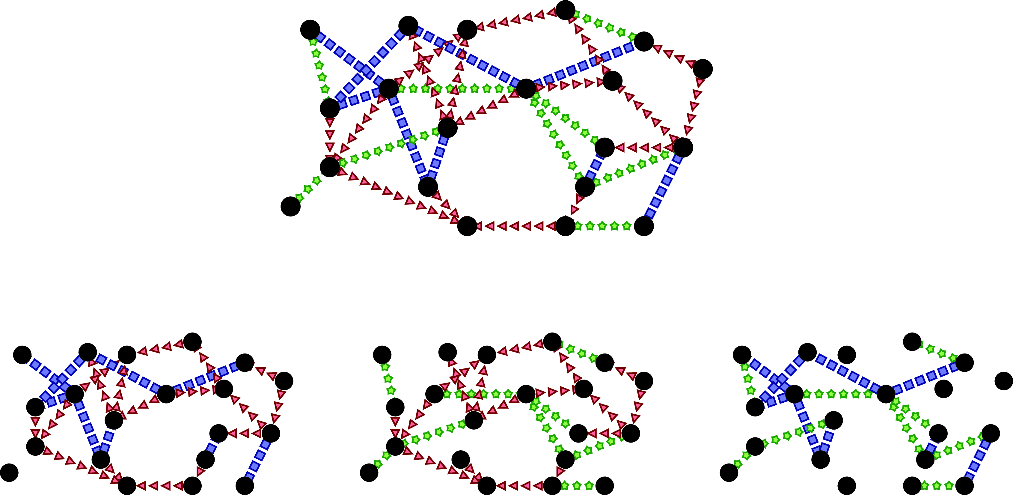
Figure 1. The colors red, blue, and green are denoted by (red) triangles, (blue) rectangles, and (green) stars, respectively. At the top, an edge-colored graph G is shown; in the second row, we can see the respective color-subgraphs $G^{\textrm{red, blue}}$
,
$G^{\textrm{red, blue}}$
, $G^{\textrm{red, green}}$
,
$G^{\textrm{red, green}}$
, $G^{\textrm{blue, green}}$
.
$G^{\textrm{blue, green}}$
.
2.1. Main results
Definition 2.3. (Color-avoiding connectivity.) Let $G = (V, \underline{E})$
be an edge-colored graph with
$G = (V, \underline{E})$
be an edge-colored graph with $k \in \mathbb{N}_+$
colors. For any color
$k \in \mathbb{N}_+$
colors. For any color $i \in [k]$
, we say that the vertices
$i \in [k]$
, we say that the vertices $v,w \in V(G)$
are i-avoiding connected, denoted by
$v,w \in V(G)$
are i-avoiding connected, denoted by $v \stackrel{G^{\setminus i}}{\longleftrightarrow} w$
, if v and w are in the same component in the graph
$v \stackrel{G^{\setminus i}}{\longleftrightarrow} w$
, if v and w are in the same component in the graph $G^{\setminus i}$
, i.e. there exists a path between v and w in G which does not contain any edges of color i; such a path is called an i-avoiding v–w path. We say that the vertices
$G^{\setminus i}$
, i.e. there exists a path between v and w in G which does not contain any edges of color i; such a path is called an i-avoiding v–w path. We say that the vertices $v,w \in V(G)$
are color-avoiding connected if they are i-avoiding connected for all
$v,w \in V(G)$
are color-avoiding connected if they are i-avoiding connected for all $i \in [k]$
.
$i \in [k]$
.
Definition 2.4. (Edge-colored Poisson branching process tree.) Let $k \in \mathbb{N}_+$
and
$k \in \mathbb{N}_+$
and $\underline{\lambda} \in \mathbb{R}^k_+$
. We say that
$\underline{\lambda} \in \mathbb{R}^k_+$
. We say that $G_{\infty} \,:\!=\, G_{\infty}(r)$
is an edge-colored Poisson branching process tree (or ECBP tree for short) with color intensity parameter vector
$G_{\infty} \,:\!=\, G_{\infty}(r)$
is an edge-colored Poisson branching process tree (or ECBP tree for short) with color intensity parameter vector $\underline{\lambda}$
, denoted by
$\underline{\lambda}$
, denoted by $G_{\infty}(r) \sim \mathcal{G}_{\infty}(\underline{\lambda})$
, if
$G_{\infty}(r) \sim \mathcal{G}_{\infty}(\underline{\lambda})$
, if $G_{\infty} = (V, \underline{E})$
is a (possibly infinite) edge-colored tree on a random vertex set V with a distinguished root vertex
$G_{\infty} = (V, \underline{E})$
is a (possibly infinite) edge-colored tree on a random vertex set V with a distinguished root vertex $r \in V$
, and with a random edge set
$r \in V$
, and with a random edge set $\underline{E} = (E_1, \ldots, E_k)$
colored with k colors, and
$\underline{E} = (E_1, \ldots, E_k)$
colored with k colors, and $G_{\infty}$
can be recursively generated in the following way. Assume that we have already generated the graph
$G_{\infty}$
can be recursively generated in the following way. Assume that we have already generated the graph $G_{\infty}$
up to the dth generation (i.e. up to graph distance d from the root) for some
$G_{\infty}$
up to the dth generation (i.e. up to graph distance d from the root) for some $d \in \mathbb{N}$
. Given a vertex v in the dth generation, let
$d \in \mathbb{N}$
. Given a vertex v in the dth generation, let $X_{v,i}$
denote the number of vertices in the
$X_{v,i}$
denote the number of vertices in the $(d+1)$
th generation which are connected to v by an edge of color i, where
$(d+1)$
th generation which are connected to v by an edge of color i, where $i \in [k]$
. Then
$i \in [k]$
. Then $X_{v,i} \sim \textrm{Poi}(\lambda_i)$
. Moreover, the family
$X_{v,i} \sim \textrm{Poi}(\lambda_i)$
. Moreover, the family $\{X_{v,i}\colon v$
is a vertex in the dth generation and
$\{X_{v,i}\colon v$
is a vertex in the dth generation and $i \in [k]\}$
of random variables are conditionally independent given the graph up to generation d.
$i \in [k]\}$
of random variables are conditionally independent given the graph up to generation d.
Since in this article all the edge-colored branching process trees have Poisson offspring distribution, we do not include the word Poisson in the abbreviation ECBP.
Definition 2.5. (Friends in ECBP trees.) Let $k \in \mathbb{N}_+$
and
$k \in \mathbb{N}_+$
and $\underline{\lambda} \in \mathbb{R}^k_+$
. Given an ECBP tree
$\underline{\lambda} \in \mathbb{R}^k_+$
. Given an ECBP tree $G_{\infty} \,:\!=\, G_{\infty}(r) \sim \mathcal{G}_\infty(\underline{\lambda})$
, a vertex
$G_{\infty} \,:\!=\, G_{\infty}(r) \sim \mathcal{G}_\infty(\underline{\lambda})$
, a vertex $v \in V(G_{\infty})$
, and a color
$v \in V(G_{\infty})$
, and a color $i \in [k]$
, we say that v is i-avoiding connected to infinity, denoted by
$i \in [k]$
, we say that v is i-avoiding connected to infinity, denoted by $v \stackrel{G_{\infty}^{\setminus i}}{\longleftrightarrow} \infty$
, if there exists an infinitely long path from v which does not contain any edges of color i and all of the vertices on this path are descendants of v. We say that the root r and the vertex v are i-avoiding friends if the event
$v \stackrel{G_{\infty}^{\setminus i}}{\longleftrightarrow} \infty$
, if there exists an infinitely long path from v which does not contain any edges of color i and all of the vertices on this path are descendants of v. We say that the root r and the vertex v are i-avoiding friends if the event
 \begin{align*} \Big\{r \stackrel{G_{\infty}^{\setminus i}}{\longleftrightarrow} v\Big\} \cup \Big(\Big\{r \stackrel{G_{\infty}^{\setminus i}}{\longleftrightarrow} \infty\Big\} \cap \Big\{v \stackrel{G_{\infty}^{\setminus i}}{\longleftrightarrow} \infty\Big\}\Big) \end{align*}
occurs. In words: r and v are i-avoiding friends if and only if there is an i-avoiding r–v path or both of them are i-avoiding connected to infinity (in which case we say that they are i-avoiding connected through infinity). We say that r and v are (color-avoiding) friends if they are i-avoiding friends for all $i \in [k]$
. The set of friends of the root r is denoted by
$i \in [k]$
. The set of friends of the root r is denoted by $\widetilde{\mathcal{C}}^*(r) \,:\!=\, \widetilde{\mathcal{C}}^*(r, G_{\infty})$
.
$\widetilde{\mathcal{C}}^*(r) \,:\!=\, \widetilde{\mathcal{C}}^*(r, G_{\infty})$
.
Note that the root r is always a friend of itself. Although the notation $\widetilde{\mathcal{C}}^*$
(which includes a tilde and an asterisk) might seem complicated, it does have a purpose, as we now explain. Throughout the paper we use a tilde to denote the generalization of a standard graph-theoretical notation (in this case the component of a vertex) to the case of color-avoiding connectivity. The asterisk reminds us that in the case of branching process trees, we are allowed to make a connection through infinity as well.
$\widetilde{\mathcal{C}}^*$
(which includes a tilde and an asterisk) might seem complicated, it does have a purpose, as we now explain. Throughout the paper we use a tilde to denote the generalization of a standard graph-theoretical notation (in this case the component of a vertex) to the case of color-avoiding connectivity. The asterisk reminds us that in the case of branching process trees, we are allowed to make a connection through infinity as well.
Definition 2.6. (Probability of $\ell$
friends in ECBP trees.) Let
$\ell$
friends in ECBP trees.) Let $k \in \mathbb{N}_+$
and
$k \in \mathbb{N}_+$
and $\underline{\lambda} \in \mathbb{R}^k_+$
. Given an ECBP tree
$\underline{\lambda} \in \mathbb{R}^k_+$
. Given an ECBP tree $G_{\infty}(r) \sim \mathcal{G}_{\infty}(\underline{\lambda})$
and
$G_{\infty}(r) \sim \mathcal{G}_{\infty}(\underline{\lambda})$
and $\ell \in \mathbb{N}_+ \cup \{ \infty \}$
, let
$\ell \in \mathbb{N}_+ \cup \{ \infty \}$
, let $f^*_{\ell} \,:\!=\, f^*_{\ell}(\underline{\lambda}) \,:\!=\, \mathbb{P}(|\widetilde{\mathcal{C}}^*(r)| = \ell)$
denote the probability that the root r has exactly
$f^*_{\ell} \,:\!=\, f^*_{\ell}(\underline{\lambda}) \,:\!=\, \mathbb{P}(|\widetilde{\mathcal{C}}^*(r)| = \ell)$
denote the probability that the root r has exactly $\ell$
friends.
$\ell$
friends.
The next claim directly follows from this definition.
Claim 2.1. (Number of friends in ECBP trees) Let $k \in \mathbb{N}_+$
,
$k \in \mathbb{N}_+$
, $\underline{\lambda} \in \mathbb{R}^k_+$
, and
$\underline{\lambda} \in \mathbb{R}^k_+$
, and $G_{\infty}(r) \sim \mathcal{G}_{\infty}(\underline{\lambda})$
an ECBP tree. Then
$G_{\infty}(r) \sim \mathcal{G}_{\infty}(\underline{\lambda})$
an ECBP tree. Then $f^*_\infty + \sum_{\ell \in \mathbb{N}_+} f^*_{\ell} = 1$
.
$f^*_\infty + \sum_{\ell \in \mathbb{N}_+} f^*_{\ell} = 1$
.
Definition 2.7. (Intensity parameters of uncolored color-subgraphs.) Let $k \in \mathbb{N}_+$
,
$k \in \mathbb{N}_+$
, $\underline{\lambda} = (\lambda_1, \ldots, \lambda_k) \in \mathbb{R}_+^k$
, and, for any
$\underline{\lambda} = (\lambda_1, \ldots, \lambda_k) \in \mathbb{R}_+^k$
, and, for any $i \in [k]$
or
$i \in [k]$
or $I \subseteq [k]$
, write
$I \subseteq [k]$
, write $\lambda_I \,:\!=\, \sum_{i \in I} \lambda_i$
,
$\lambda_I \,:\!=\, \sum_{i \in I} \lambda_i$
, $\lambda^{\textrm{uc}} \,:\!=\, \lambda_{[k]}$
, and
$\lambda^{\textrm{uc}} \,:\!=\, \lambda_{[k]}$
, and $\lambda^{\setminus i} \,:\!=\, \lambda_{[k] \setminus \{ i \}}$
.
$\lambda^{\setminus i} \,:\!=\, \lambda_{[k] \setminus \{ i \}}$
.
Definition 2.8. (Fully supercritical/critical-subcritical $\underline{\lambda}$
.) Let
$\underline{\lambda}$
.) Let $k \in \mathbb{N}_+$
. We say that a vector
$k \in \mathbb{N}_+$
. We say that a vector $\underline{\lambda} \in \mathbb{R}_+^k$
is fully supercritical if
$\underline{\lambda} \in \mathbb{R}_+^k$
is fully supercritical if $\lambda^{\setminus i} > 1$
for all
$\lambda^{\setminus i} > 1$
for all $i \in [k]$
, and we say that
$i \in [k]$
, and we say that $\underline{\lambda}$
is fully critical-subcritical if
$\underline{\lambda}$
is fully critical-subcritical if $\lambda^{\setminus i} \le 1$
for all
$\lambda^{\setminus i} \le 1$
for all $i \in [k]$
.
$i \in [k]$
.
Note that a vector might be neither fully supercritical nor fully critical-subcritical. In Section 4.2, we make the following simplifying assumption on the color intensity parameter vector $\underline{\lambda}$
.
$\underline{\lambda}$
.
Assumption 2.1. (Simplifying assumption.) Let $k \in \mathbb{N}_+$
,
$k \in \mathbb{N}_+$
, $k \ge 2$
, let
$k \ge 2$
, let $\underline{\lambda} \in \mathbb{R}_+^k$
, and assume that
$\underline{\lambda} \in \mathbb{R}_+^k$
, and assume that $\lambda_I < 1$
for any
$\lambda_I < 1$
for any $I \subseteq [k]$
with
$I \subseteq [k]$
with $|I| \le k-2$
.
$|I| \le k-2$
.
Heuristically, if $\underline{\lambda}$
is fully supercritical and Assumption 2.1 holds, then we really need to use all of the other
$\underline{\lambda}$
is fully supercritical and Assumption 2.1 holds, then we really need to use all of the other $k-1$
colors to create an infinitely long i-avoiding path for each
$k-1$
colors to create an infinitely long i-avoiding path for each $i \in [k]$
in an ECBP tree.
$i \in [k]$
in an ECBP tree.
Proposition 2.1. (Characterization of positivity of $f^*_{\infty}$
.) Let
$f^*_{\infty}$
.) Let $k \in \mathbb{N}_+$
. A vector
$k \in \mathbb{N}_+$
. A vector $\underline{\lambda} \in \mathbb{R}_+^k$
is fully supercritical if and only if
$\underline{\lambda} \in \mathbb{R}_+^k$
is fully supercritical if and only if $f^*_{\infty} > 0$
.
$f^*_{\infty} > 0$
.
We prove Proposition 2.1 in Section 3.2. In Section 4, we provide formulas for $f^*_{\infty}$
. These formulas are explicit in the sense that they can be obtained by a recursive composition of elementary functions and the Lambert W function. The depth of our recursive formulas increases as the number k of colors increases. We provide two different methods for the calculation of
$f^*_{\infty}$
. These formulas are explicit in the sense that they can be obtained by a recursive composition of elementary functions and the Lambert W function. The depth of our recursive formulas increases as the number k of colors increases. We provide two different methods for the calculation of $f^*_{\infty}$
: the method described in Section 4.1 works even if we do not assume Assumption 2.1, while the method described in Section 4.2 only works under Assumption 2.1, but it can be used to study the asymptotic behavior of
$f^*_{\infty}$
: the method described in Section 4.1 works even if we do not assume Assumption 2.1, while the method described in Section 4.2 only works under Assumption 2.1, but it can be used to study the asymptotic behavior of $f^*_{\infty}$
in the barely supercritical regime, cf. Theorem 2.1.
$f^*_{\infty}$
in the barely supercritical regime, cf. Theorem 2.1.
Proposition 2.2. (Characterization of positivity of $f_{\ell}^*$
.) Let
$f_{\ell}^*$
.) Let $k \in \mathbb{N}_+$
and let
$k \in \mathbb{N}_+$
and let $\underline{\lambda} \in \mathbb{R}_+^k$
for which Assumption 2.1 holds.
$\underline{\lambda} \in \mathbb{R}_+^k$
for which Assumption 2.1 holds.
-
(i) If $\underline{\lambda}$
is fully critical-subcritical, then
$f^*_{\ell} = \textbf{1}[\ell=1]$
for any
$\ell \in \mathbb{N}_+$
.
$\underline{\lambda}$
is fully critical-subcritical, then
$f^*_{\ell} = \textbf{1}[\ell=1]$
for any
$\ell \in \mathbb{N}_+$
. -
(ii) If
$\underline{\lambda}$
is not fully critical-subcritical, then
$f^*_{\ell} > 0$
for any
$\ell \in \mathbb{N}_+$
.


We prove Proposition 2.2 in Section 3.2.
A vector $\underline{\lambda} = (\lambda_1, \ldots, \lambda_k) \in \mathbb{R}_+^k$
for some integer
$\underline{\lambda} = (\lambda_1, \ldots, \lambda_k) \in \mathbb{R}_+^k$
for some integer $k \ge 2$
is called homogeneous if
$k \ge 2$
is called homogeneous if $\lambda_1 = \ldots = \lambda_k$
.
$\lambda_1 = \ldots = \lambda_k$
.
Definition 2.9. (Barely supercritical homogeneous setup.) Let $k \in \mathbb{N}_+$
,
$k \in \mathbb{N}_+$
, $k \ge 2$
. For any
$k \ge 2$
. For any $\varepsilon \ge 0$
, we define
$\varepsilon \ge 0$
, we define
 \begin{align*} \underline{\lambda}(\varepsilon) \,:\!=\, \bigg(\frac{1+\varepsilon}{k-1}, \ldots, \frac{1+\varepsilon}{k-1}\bigg) \in \mathbb{R}_+^k \end{align*}
and $f^*_{\infty}(\varepsilon) \,:\!=\, f^*_{\infty}(\underline{\lambda}(\varepsilon))$
.
$f^*_{\infty}(\varepsilon) \,:\!=\, f^*_{\infty}(\underline{\lambda}(\varepsilon))$
.
Note that if $\varepsilon > 0$
, then
$\varepsilon > 0$
, then $f^*_{\infty}(\varepsilon) > 0$
, but if
$f^*_{\infty}(\varepsilon) > 0$
, but if $\varepsilon = 0$
, then
$\varepsilon = 0$
, then $f^*_{\infty}(\varepsilon) = 0$
by Proposition 2.1. Also note that if
$f^*_{\infty}(\varepsilon) = 0$
by Proposition 2.1. Also note that if $\varepsilon < {1}/({k-2})$
then Assumption 2.1 holds for
$\varepsilon < {1}/({k-2})$
then Assumption 2.1 holds for $\underline{\lambda}(\varepsilon)$
.
$\underline{\lambda}(\varepsilon)$
.
Our next result is about the asymptotic behavior of $f^*_{\infty}(\varepsilon)$
as
$f^*_{\infty}(\varepsilon)$
as $\varepsilon \to 0_+$
.
$\varepsilon \to 0_+$
.
Theorem 2.1. (Asymptotic decay of the probability of having infinitely many friends in the barely supercritical homogeneous setup.) Let $k \in \mathbb{N}_+$
,
$k \in \mathbb{N}_+$
, $k \geq 2$
. Then there exists a constant
$k \geq 2$
. Then there exists a constant $C(k) \in \mathbb{R}_+$
such that
$C(k) \in \mathbb{R}_+$
such that $\lim_{\varepsilon \to 0_+} {f^*_{\infty}(\varepsilon)}/{\varepsilon^k} = C(k)$
. In particular,
$\lim_{\varepsilon \to 0_+} {f^*_{\infty}(\varepsilon)}/{\varepsilon^k} = C(k)$
. In particular, $C(2)= 4$
,
$C(2)= 4$
, $C(3)=32$
, and
$C(3)=32$
, and $C(4)=624$
.
$C(4)=624$
.
In Section 4, we provide a method for computing the value of C(k) for any integer $k \ge 2$
and prove Theorem 2.1.
$k \ge 2$
and prove Theorem 2.1.
2.2. Context
In the following, we give some motivation for studying the above problems on ECBP trees. As is known (see, e.g., [Reference Van der Hofstad31]), branching process trees arise as local limits of Erdős–Rényi graphs. We show that, analogously, ECBP trees can be used for studying color-avoiding percolation in edge-colored Erdős–Rényi multigraphs.
Definition 2.10. (Edge-colored Erdős–Rényi multigraph.) Let $k,n \in \mathbb{N}_+$
and
$k,n \in \mathbb{N}_+$
and $\underline{\lambda} = (\lambda_1,\ldots,\lambda_k) \in \mathbb{R}_+^k$
. We say that the edge-colored random multigraph
$\underline{\lambda} = (\lambda_1,\ldots,\lambda_k) \in \mathbb{R}_+^k$
. We say that the edge-colored random multigraph $G = (V, \underline{E})$
is an edge-colored Erdős–Rényi multigraph (or ECER graph for short) with parameter n and color density parameter vector
$G = (V, \underline{E})$
is an edge-colored Erdős–Rényi multigraph (or ECER graph for short) with parameter n and color density parameter vector $\underline{\lambda}$
, denoted by
$\underline{\lambda}$
, denoted by $G \sim \mathcal{G}_n (V, \underline{\lambda})$
, if
$G \sim \mathcal{G}_n (V, \underline{\lambda})$
, if $|V| \le n$
and
$|V| \le n$
and $\underline{E}=(E_1, \ldots, E_k)$
, where
$\underline{E}=(E_1, \ldots, E_k)$
, where $E_1, \ldots, E_k$
are independent in the stochastic sense and
$E_1, \ldots, E_k$
are independent in the stochastic sense and $E_i$
is the edge set of an Erdős–Rényi graph with vertex set V and edge probability
$E_i$
is the edge set of an Erdős–Rényi graph with vertex set V and edge probability $p_i = 1 - \exp({-}\lambda_i/n)$
(i.e. each possible edge of
$p_i = 1 - \exp({-}\lambda_i/n)$
(i.e. each possible edge of $\binom{V}{2}$
is included in
$\binom{V}{2}$
is included in $E_i$
independently of each other with probability
$E_i$
independently of each other with probability $p_i$
) for all
$p_i$
) for all $i \in [k]$
.
$i \in [k]$
.
Clearly, the relation of color-avoiding connectivity (cf. Definition 2.3) is an equivalence relation and thus it defines a partition of the vertex set.
Definition 2.11. (Color-avoiding connected components.) The equivalence classes of the relation of color-avoiding connectivity are called color-avoiding connected components. The set of vertices of the color-avoiding connected component of a vertex v in an edge-colored graph G is denoted by $\widetilde{\mathcal{C}}(v) \,:\!=\, \widetilde{\mathcal{C}}(v,G)$
.
$\widetilde{\mathcal{C}}(v) \,:\!=\, \widetilde{\mathcal{C}}(v,G)$
.
Recall that the tilde above $\widetilde{\mathcal{C}}(v)$
is there to stress that the standard notion of the connected component of graph theory is generalized to the color-avoiding framework.
$\widetilde{\mathcal{C}}(v)$
is there to stress that the standard notion of the connected component of graph theory is generalized to the color-avoiding framework.
Note that even if v and w are in the same color-avoiding connected component $\widetilde{\mathcal{C}}$
, it might still happen that there exists a color i for which every i-avoiding v–w path has vertices outside
$\widetilde{\mathcal{C}}$
, it might still happen that there exists a color i for which every i-avoiding v–w path has vertices outside $\widetilde{\mathcal{C}}$
. For an example, see Figure 2.
$\widetilde{\mathcal{C}}$
. For an example, see Figure 2.
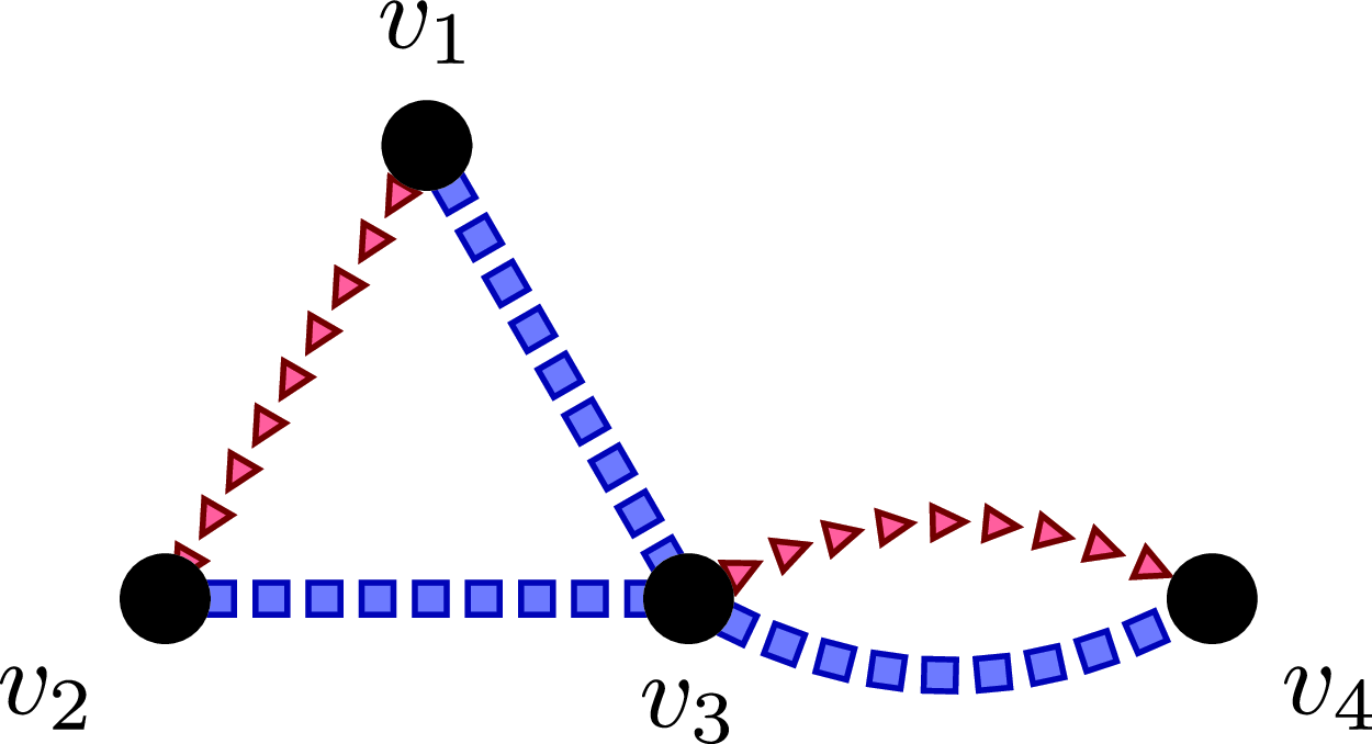
Figure 2. The colors red and blue are denoted by (red) triangles and (blue) rectangles, respectively. The color-avoiding connected components of this graph are $\{ v_1, v_2 \}$
and
$\{ v_1, v_2 \}$
and $\{ v_3, v_4 \}$
. Note that the red-avoiding
$\{ v_3, v_4 \}$
. Note that the red-avoiding $v_1$
–
$v_1$
– $v_2$
path leaves the component
$v_2$
path leaves the component $\{ v_1, v_2 \}$
.
$\{ v_1, v_2 \}$
.
Definition 2.12. (Empirical density of vertices in color-avoiding connected components of size $\ell$
.) Let
$\ell$
.) Let $k \in \mathbb{N}_+$
and
$k \in \mathbb{N}_+$
and $\underline{\lambda} \in \mathbb{R}^k_+$
. Given an ECER graph
$\underline{\lambda} \in \mathbb{R}^k_+$
. Given an ECER graph $G \sim \mathcal{G}_n ([n], \underline{\lambda})$
, let
$G \sim \mathcal{G}_n ([n], \underline{\lambda})$
, let
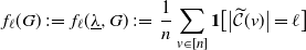 \begin{align*} f_{\ell}(G) \,:\!=\, f_{\ell}(\underline{\lambda}, G) \,:\!=\, \frac{1}{n}\sum_{v \in [n]}\textbf{1}\big[\big|\widetilde{\mathcal{C}}(v)\big| = \ell\big] \end{align*}
denote the fraction of vertices contained in color-avoiding connected components of size $\ell$
for any
$\ell$
for any $\ell \in \mathbb{N}_+$
.
$\ell \in \mathbb{N}_+$
.
The next claim directly follows from this definition.
Claim 2.2. (Size of color-avoiding connected components in ECER graphs.) Let $k, n \in \mathbb{N}_+$
,
$k, n \in \mathbb{N}_+$
, $\underline{\lambda} \in \mathbb{R}^k_+$
, and
$\underline{\lambda} \in \mathbb{R}^k_+$
, and $G \sim \mathcal{G}_n([n],\underline{\lambda})$
an ECER graph. Then
$G \sim \mathcal{G}_n([n],\underline{\lambda})$
an ECER graph. Then $\sum_{\ell \in [n]}f_{\ell}(G) = 1$
.
$\sum_{\ell \in [n]}f_{\ell}(G) = 1$
.
Theorem 2.2. (Convergence of empirical component size densities.) Let $k \in \mathbb{N}_+$
,
$k \in \mathbb{N}_+$
, $\underline{\lambda} \in \mathbb{R}_+^k$
, and let
$\underline{\lambda} \in \mathbb{R}_+^k$
, and let $G_n \sim \mathcal{G}_n([n],\underline{\lambda})$
for all
$G_n \sim \mathcal{G}_n([n],\underline{\lambda})$
for all $n \in \mathbb{N}_+$
. Then
$n \in \mathbb{N}_+$
. Then $({1}/{n})\max_{v \in [n]}\big|\widetilde{\mathcal{C}}\big(v, G_n\big)\big| \stackrel{\mathbb{P}}{\longrightarrow} f^*_\infty$
as
$({1}/{n})\max_{v \in [n]}\big|\widetilde{\mathcal{C}}\big(v, G_n\big)\big| \stackrel{\mathbb{P}}{\longrightarrow} f^*_\infty$
as $n \to \infty$
and, for any
$n \to \infty$
and, for any $\ell \in \mathbb{N}_+$
,
$\ell \in \mathbb{N}_+$
, $f_{\ell}(G_n) \stackrel{\mathbb{P}}{\longrightarrow} f^*_{\ell}$
as
$f_{\ell}(G_n) \stackrel{\mathbb{P}}{\longrightarrow} f^*_{\ell}$
as $n \to \infty$
.
$n \to \infty$
.
Theorem 2.2 is proved in an earlier version of this paper [Reference Ráth26] using Assumption 2.1, and a short alternative proof is given in [Reference Lichev and Schapira20] without using Assumption 2.1.
From Theorem 2.2 and Claim 2.1, we can conclude the following.
Corollary 2.1. (Existence and uniqueness of a giant color-avoiding connected component in ECER graphs.) Let $k, n \in \mathbb{N}_+$
,
$k, n \in \mathbb{N}_+$
, $\underline{\lambda} \in \mathbb{R}_+^k$
, and let
$\underline{\lambda} \in \mathbb{R}_+^k$
, and let $G_n \sim \mathcal{G}_n([n],\underline{\lambda})$
. If
$G_n \sim \mathcal{G}_n([n],\underline{\lambda})$
. If $f^*_{\infty} > 0$
, then
$f^*_{\infty} > 0$
, then $G_n$
has a unique largest color-avoiding connected component asymptotically almost surely as
$G_n$
has a unique largest color-avoiding connected component asymptotically almost surely as $n \to \infty$
.
$n \to \infty$
.
Note that Theorem 2.2 provides the motivation for the main results of this paper: Proposition 2.1 gives a characterization of the existence of the giant color-avoiding connected component in ECER graphs and Proposition 2.2 characterizes the case when the fraction of vertices of an ECER graph contained in singleton color-avoiding components is close to 1.
We note that [Reference Lichev and Schapira20] includes results about the size of the largest color-avoiding component for certain parameter vectors $\underline{\lambda}$
which are neither fully supercritical nor fully critical-subcritical (see [Reference Lichev and Schapira20, Theorem 1.1(ii)]) as well as fully subcritical vectors
$\underline{\lambda}$
which are neither fully supercritical nor fully critical-subcritical (see [Reference Lichev and Schapira20, Theorem 1.1(ii)]) as well as fully subcritical vectors $\underline{\lambda}$
(see [Reference Lichev and Schapira20, Theorem 1.1(iii)]).
$\underline{\lambda}$
(see [Reference Lichev and Schapira20, Theorem 1.1(iii)]).
3. Preliminaries
In this section, we introduce some notation that we use throughout the paper; moreover, we prove Propositions 2.1 and 2.2.
3.1. Notation
We say that two edge-colored graphs $G_1$
and
$G_1$
and $G_2$
are isomorphic, denoted by
$G_2$
are isomorphic, denoted by $G_1 \simeq G_2$
, if there exists a bijection between their vertex sets which is an isomorphism for the set of edges of each color.
$G_1 \simeq G_2$
, if there exists a bijection between their vertex sets which is an isomorphism for the set of edges of each color.
We say that an edge-colored graph is rooted if it has a distinguished vertex. We say that the rooted edge-colored graphs $G_1$
and
$G_1$
and $G_2$
with distinguished vertices
$G_2$
with distinguished vertices $v_1$
and
$v_1$
and $v_2$
, respectively, are isomorphic if there exists an isomorphism between them mapping
$v_2$
, respectively, are isomorphic if there exists an isomorphism between them mapping $v_1$
to
$v_1$
to $v_2$
.
$v_2$
.
Let $G=(V,E)$
be a graph without an edge-coloring. For a vertex
$G=(V,E)$
be a graph without an edge-coloring. For a vertex $v \in V$
, let
$v \in V$
, let $\mathcal{C}(v) \,:\!=\, \mathcal{C}(v,G)$
denote the set of vertices of the connected component of v in G.
$\mathcal{C}(v) \,:\!=\, \mathcal{C}(v,G)$
denote the set of vertices of the connected component of v in G.
For two vertices $v,w \in V(G)$
, let
$v,w \in V(G)$
, let $\textrm{dist}(v,w) \,:\!=\, \textrm{dist}_G(v,w)$
denote the distance of v and w (i.e. the number of edges on a shortest v–w path) in G.
$\textrm{dist}(v,w) \,:\!=\, \textrm{dist}_G(v,w)$
denote the distance of v and w (i.e. the number of edges on a shortest v–w path) in G.
Definition 3.1. (Color strings of length h without repetition.) Let $k \in \mathbb{N}_+$
and let
$k \in \mathbb{N}_+$
and let $h \in \{ 0, 1, \ldots, k \}$
. Let
$h \in \{ 0, 1, \ldots, k \}$
. Let $S_h$
denote the set of strings
$S_h$
denote the set of strings $\underline{s} = (i_1, \ldots, i_h)$
of colors without any repetition, i.e.
$\underline{s} = (i_1, \ldots, i_h)$
of colors without any repetition, i.e. $i_1, \ldots, i_h \in [k]$
and
$i_1, \ldots, i_h \in [k]$
and $|\{ i_1, \ldots, i_h \}| = h$
; the set
$|\{ i_1, \ldots, i_h \}| = h$
; the set $S_0$
has one element, namely the empty string
$S_0$
has one element, namely the empty string $\emptyset$
. We define
$\emptyset$
. We define $\textrm{set}(\underline{s}) \,:\!=\, \{ i_1, \ldots, i_h \}$
for a string
$\textrm{set}(\underline{s}) \,:\!=\, \{ i_1, \ldots, i_h \}$
for a string $\underline{s} = (i_1, \ldots, i_h) \in S_h$
.
$\underline{s} = (i_1, \ldots, i_h) \in S_h$
.
Note that $|S_h| = k \cdot (k-1) \cdots (k-h+1)$
for any
$|S_h| = k \cdot (k-1) \cdots (k-h+1)$
for any $h \in [k]$
.
$h \in [k]$
.
Definition 3.2. (Color string operations.) Let $k \in \mathbb{N}_+$
. For any color string
$k \in \mathbb{N}_+$
. For any color string $\underline{s} = (i_1, \ldots, i_h) \in S_h$
, where
$\underline{s} = (i_1, \ldots, i_h) \in S_h$
, where $h \in [k]$
, let
$h \in [k]$
, let $\underline{s}^- \,:\!=\, (i_1, \ldots, i_{h-1}) \in S_{h-1}$
denote the color string that can be obtained from
$\underline{s}^- \,:\!=\, (i_1, \ldots, i_{h-1}) \in S_{h-1}$
denote the color string that can be obtained from $\underline{s}$
by deleting its last coordinate. For any
$\underline{s}$
by deleting its last coordinate. For any $\underline{s} = (i_1, \ldots, i_h) \in S_h$
, where
$\underline{s} = (i_1, \ldots, i_h) \in S_h$
, where $h \in \{ 0, 1, \ldots,$ $k-1 \}$
, and for any
$k-1 \}$
, and for any $i \in [k] \setminus \textrm{set}(\underline{s})$
, let
$i \in [k] \setminus \textrm{set}(\underline{s})$
, let $\underline{s}i \,:\!=\, (i_1, \ldots, i_h, i) \in S_{h+1}$
denote the concatenation of
$\underline{s}i \,:\!=\, (i_1, \ldots, i_h, i) \in S_{h+1}$
denote the concatenation of $\underline{s}$
and i.
$\underline{s}$
and i.
Definition 3.3. (Set of vertices reachable by a fixed chronology of colors.) For an edge-colored rooted tree $G \,:\!=\, G(r)$
colored with
$G \,:\!=\, G(r)$
colored with $k \in \mathbb{N}_+$
colors, and a color string
$k \in \mathbb{N}_+$
colors, and a color string $\underline{s} = (i_1, \ldots, i_h) \in S_h$
, where
$\underline{s} = (i_1, \ldots, i_h) \in S_h$
, where $h \in [k]$
, we define the following sets of vertices. Let
$h \in [k]$
, we define the following sets of vertices. Let $\widetilde{R}_{\underline{s}}(r) \,:\!=\, \widetilde{R}_{\underline{s}}(r,G)$
denote the set of vertices that can be reached from r with a path whose edges are of color
$\widetilde{R}_{\underline{s}}(r) \,:\!=\, \widetilde{R}_{\underline{s}}(r,G)$
denote the set of vertices that can be reached from r with a path whose edges are of color $i_1, \ldots, i_h$
and the new colors on this path appear in this specific order. Let
$i_1, \ldots, i_h$
and the new colors on this path appear in this specific order. Let $\widetilde{N}_{\underline{s}}(r) \,:\!=\, \widetilde{N}_{\underline{s}}(r,G)$
denote the set of vertices that can be reached from r with a path whose edges, except the last one, are of color
$\widetilde{N}_{\underline{s}}(r) \,:\!=\, \widetilde{N}_{\underline{s}}(r,G)$
denote the set of vertices that can be reached from r with a path whose edges, except the last one, are of color $i_1, \ldots, i_{h-1}$
, the last edge is of color
$i_1, \ldots, i_{h-1}$
, the last edge is of color $i_h$
, and the new colors on this path appear in this specific order. In addition, let
$i_h$
, and the new colors on this path appear in this specific order. In addition, let
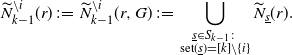 \begin{align*} \widetilde{N}_{k-1}^{\setminus i}(r) \,:\!=\, \widetilde{N}_{k-1}^{\setminus i}(r,G) \,:\!=\, \bigcup_{\substack{\underline{s}\in S_{k-1}\colon\\\textrm{set}(\underline{s})=[k]\setminus\{i\}}}\widetilde{N}_{\underline{s}}(r). \end{align*}
For an example, see Figure 3.
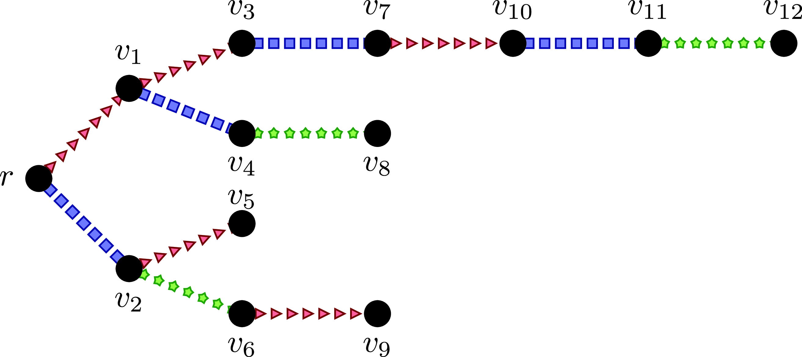
Figure 3. The colors red, blue, and green are denoted by (red) triangles, (blue) rectangles, and (green) stars, respectively. In this graph, $\widetilde{R}_{(\textrm{red})}(r) = \{ v_1, v_3 \}$
,
$\widetilde{R}_{(\textrm{red})}(r) = \{ v_1, v_3 \}$
, $\widetilde{R}_{(\textrm{blue})}(r) = \{ v_2 \}$
,
$\widetilde{R}_{(\textrm{blue})}(r) = \{ v_2 \}$
, $\widetilde{R}_{(\textrm{green})}(r) = \emptyset$
,
$\widetilde{R}_{(\textrm{green})}(r) = \emptyset$
, $\widetilde{R}_{(\textrm{red}, \textrm{blue})}(r) = \{ v_4, v_7, v_{10}, v_{11} \}$
, and
$\widetilde{R}_{(\textrm{red}, \textrm{blue})}(r) = \{ v_4, v_7, v_{10}, v_{11} \}$
, and $\widetilde{R}_{(\textrm{blue}, \textrm{red})}(r) = \{ v_5 \}$
;
$\widetilde{R}_{(\textrm{blue}, \textrm{red})}(r) = \{ v_5 \}$
; $\widetilde{R}_{(\textrm{red}, \textrm{blue}, \textrm{green})}(r) = \{ v_8, v_{12} \}$
and
$\widetilde{R}_{(\textrm{red}, \textrm{blue}, \textrm{green})}(r) = \{ v_8, v_{12} \}$
and $\widetilde{R}_{(\textrm{blue}, \textrm{green}, \textrm{red})}(r) = \{ v_9 \}$
;
$\widetilde{R}_{(\textrm{blue}, \textrm{green}, \textrm{red})}(r) = \{ v_9 \}$
; $\widetilde{N}_{(\textrm{red})}(r) = \{ v_1 \}$
,
$\widetilde{N}_{(\textrm{red})}(r) = \{ v_1 \}$
, $\widetilde{N}_{(\textrm{red}, \textrm{blue})}(r) = \{ v_4, v_7 \}$
, and
$\widetilde{N}_{(\textrm{red}, \textrm{blue})}(r) = \{ v_4, v_7 \}$
, and $\widetilde{N}_{(\textrm{red}, \textrm{blue}, \textrm{green})}(r) = \{ v_8, v_{12} \}$
.
$\widetilde{N}_{(\textrm{red}, \textrm{blue}, \textrm{green})}(r) = \{ v_8, v_{12} \}$
.
Definition 3.4. (Exploring up to distance d.) Let $G = (V,E)$
be a graph,
$G = (V,E)$
be a graph, $v \in V$
a vertex, and
$v \in V$
a vertex, and $d \in \mathbb{N}$
. We define
$d \in \mathbb{N}$
. We define $R_d(v) \,:\!=\, R_d(v,G) \,:\!=\, \{u \in V \colon \textrm{dist}(u,v) = d\}$
, i.e. the set of vertices of G at distance d from the root, and let
$R_d(v) \,:\!=\, R_d(v,G) \,:\!=\, \{u \in V \colon \textrm{dist}(u,v) = d\}$
, i.e. the set of vertices of G at distance d from the root, and let $R^{\le}_d(v) \,:\!=\, R^{\le}_d(v,G) \,:\!=\, \{u \in V \colon \textrm{dist}(u,v) \le d\}$
, i.e. the set of vertices of G at distance at most d from the root. For an ECBP tree
$R^{\le}_d(v) \,:\!=\, R^{\le}_d(v,G) \,:\!=\, \{u \in V \colon \textrm{dist}(u,v) \le d\}$
, i.e. the set of vertices of G at distance at most d from the root. For an ECBP tree $G_{\infty} \,:\!=\, G_{\infty}(r) \sim \mathcal{G}_{\infty}(\underline{\lambda})$
, where
$G_{\infty} \,:\!=\, G_{\infty}(r) \sim \mathcal{G}_{\infty}(\underline{\lambda})$
, where $\lambda \in \mathbb{R}_+^k$
for some
$\lambda \in \mathbb{R}_+^k$
for some $k \in \mathbb{N}_+$
, and for a color
$k \in \mathbb{N}_+$
, and for a color $i \in [k]$
or for a subset of colors
$i \in [k]$
or for a subset of colors $I \subseteq [k]$
, we use the notation
$I \subseteq [k]$
, we use the notation $R_{\infty,d}^I \,:\!=\, R_d \big(r, G_{\infty}^I \big)$
,
$R_{\infty,d}^I \,:\!=\, R_d \big(r, G_{\infty}^I \big)$
, $R_{\infty,d}^{\setminus i} \,:\!=\, R_{\infty,d}^{[k] \setminus \{ i \}}$
.
$R_{\infty,d}^{\setminus i} \,:\!=\, R_{\infty,d}^{[k] \setminus \{ i \}}$
.
The next claim directly follows from the definition of ECBP trees (cf. Definition 2.4).
Lemma 3.1. (Distribution of uncolored color-subtrees of ECBP trees.) Let $k \in \mathbb{N}_+$
,
$k \in \mathbb{N}_+$
, $\underline{\lambda} \in \mathbb{R}_+^k$
, and let
$\underline{\lambda} \in \mathbb{R}_+^k$
, and let $G_{\infty}(r) \sim \mathcal{G}_{\infty}(\underline{\lambda})$
. Then
$G_{\infty}(r) \sim \mathcal{G}_{\infty}(\underline{\lambda})$
. Then $\big(\big|R_{\infty,d}^I\big|\big)_{d\in\mathbb{N}}$
is a branching process with offspring distribution
$\big(\big|R_{\infty,d}^I\big|\big)_{d\in\mathbb{N}}$
is a branching process with offspring distribution $\textrm{Poi}(\lambda_I)$
for any
$\textrm{Poi}(\lambda_I)$
for any $I \subseteq [k]$
. In particular,
$I \subseteq [k]$
. In particular, $\big( \big| R_{\infty,d}^{\setminus i} \big| \big)_{d \in \mathbb{N}}$
is a branching process with offspring distribution
$\big( \big| R_{\infty,d}^{\setminus i} \big| \big)_{d \in \mathbb{N}}$
is a branching process with offspring distribution $\textrm{Poi}(\lambda^{\setminus i})$
for any
$\textrm{Poi}(\lambda^{\setminus i})$
for any $i \in [k]$
.
$i \in [k]$
.
Definition 3.5. (Probability of being i-avoiding connected to infinity.) Let $k \in \mathbb{N}_+$
,
$k \in \mathbb{N}_+$
, $i \in [k]$
, and let
$i \in [k]$
, and let $\underline{\lambda} \in \mathbb{R}^k_+$
. We denote by
$\underline{\lambda} \in \mathbb{R}^k_+$
. We denote by $\theta^{\setminus i}$
the survival probability of the branching process with offspring distribution
$\theta^{\setminus i}$
the survival probability of the branching process with offspring distribution $\textrm{Poi}(\lambda^{\setminus i})$
.
$\textrm{Poi}(\lambda^{\setminus i})$
.
Note that if $G_{\infty} \,:\!=\, G_{\infty}(r) \sim \mathcal{G}_{\infty}(\underline{\lambda})$
then, by Lemma 3.1,
$G_{\infty} \,:\!=\, G_{\infty}(r) \sim \mathcal{G}_{\infty}(\underline{\lambda})$
then, by Lemma 3.1, $\theta^{\setminus i} = \mathbb{P}\Big(r \stackrel{G_{\infty}^{\setminus i}}{\longleftrightarrow} \infty\Big)$
.
$\theta^{\setminus i} = \mathbb{P}\Big(r \stackrel{G_{\infty}^{\setminus i}}{\longleftrightarrow} \infty\Big)$
.
Definition 3.6. (Supercritical indices.) Let $k \in \mathbb{N}_+$
. Given
$k \in \mathbb{N}_+$
. Given $\underline{\lambda} \in \mathbb{R}_+^k$
, we say that
$\underline{\lambda} \in \mathbb{R}_+^k$
, we say that $i \in [k]$
is a supercritical index if
$i \in [k]$
is a supercritical index if $\lambda^{\setminus i} > 1$
, and we define the set
$\lambda^{\setminus i} > 1$
, and we define the set $I_{\underline{\lambda}}$
of supercritical indices of
$I_{\underline{\lambda}}$
of supercritical indices of $\underline{\lambda}$
by
$\underline{\lambda}$
by $I_{\underline{\lambda}} \,:\!=\, \{ i \in [k] \colon \lambda^{\setminus i} > 1\}$
.
$I_{\underline{\lambda}} \,:\!=\, \{ i \in [k] \colon \lambda^{\setminus i} > 1\}$
.
Note that $\underline{\lambda}$
is fully supercritical (cf. Definition 2.8) if and only if
$\underline{\lambda}$
is fully supercritical (cf. Definition 2.8) if and only if $I_{\underline{\lambda}} = [k]$
, and
$I_{\underline{\lambda}} = [k]$
, and $\underline{\lambda}$
is fully critical-subcritical if and only if
$\underline{\lambda}$
is fully critical-subcritical if and only if $I_{\underline{\lambda}} = \emptyset$
. Also note that
$I_{\underline{\lambda}} = \emptyset$
. Also note that $\theta^{\setminus i} = 0$
holds if and only if
$\theta^{\setminus i} = 0$
holds if and only if $i \in [k] \setminus I_{\underline{\lambda}}$
.
$i \in [k] \setminus I_{\underline{\lambda}}$
.
Definition 3.7. (Type vectors and their probabilities in ECBP trees.) Let $k \in \mathbb{N}_+$
,
$k \in \mathbb{N}_+$
, $\underline{\lambda} \in \mathbb{R}_+^k$
, and let
$\underline{\lambda} \in \mathbb{R}_+^k$
, and let $G_{\infty} \,:\!=\, G_{\infty}(r) \sim \mathcal{G}_{\infty}(\underline{\lambda})$
. The (color-avoiding) type vector of a vertex v in the ECBP tree
$G_{\infty} \,:\!=\, G_{\infty}(r) \sim \mathcal{G}_{\infty}(\underline{\lambda})$
. The (color-avoiding) type vector of a vertex v in the ECBP tree $G_{\infty}$
is
$G_{\infty}$
is $\underline{t}^*(v) \,:\!=\, \underline{t}^*(v, G_{\infty}) \,:\!=\, \Big(\textbf{1}\Big[v \stackrel{G_{\infty}^{\setminus i}}{\longleftrightarrow} \infty\Big]\Big)_{i\in I_{\underline{\lambda}}}$
. Given any
$\underline{t}^*(v) \,:\!=\, \underline{t}^*(v, G_{\infty}) \,:\!=\, \Big(\textbf{1}\Big[v \stackrel{G_{\infty}^{\setminus i}}{\longleftrightarrow} \infty\Big]\Big)_{i\in I_{\underline{\lambda}}}$
. Given any $\underline{\gamma} \in \{ 0,1\}^{I_{\underline{\lambda}}}$
, we write
$\underline{\gamma} \in \{ 0,1\}^{I_{\underline{\lambda}}}$
, we write $p^*(\underline{\gamma}) \,:\!=\, p^*(\underline{\gamma},\underline{\lambda}) \,:\!=\, \mathbb{P}\big(\underline{t}^*(r)=\underline{\gamma}\big)$
.
$p^*(\underline{\gamma}) \,:\!=\, p^*(\underline{\gamma},\underline{\lambda}) \,:\!=\, \mathbb{P}\big(\underline{t}^*(r)=\underline{\gamma}\big)$
.
In words: for any $i \in I_{\underline{\lambda}}$
, the ith coordinate of the type vector of a vertex v in an ECBP tree is 1 if v is i-avoiding connected to infinity through its descendants, otherwise it is 0. The reason we only use the indices in
$i \in I_{\underline{\lambda}}$
, the ith coordinate of the type vector of a vertex v in an ECBP tree is 1 if v is i-avoiding connected to infinity through its descendants, otherwise it is 0. The reason we only use the indices in $I_{\underline{\lambda}}$
is that we expect the branching process
$I_{\underline{\lambda}}$
is that we expect the branching process $G_{\infty}$
to survive without the edges of color i if and only if
$G_{\infty}$
to survive without the edges of color i if and only if $i \in I_{\underline{\lambda}}$
.
$i \in I_{\underline{\lambda}}$
.
3.2. Characterization of existence of giant and nontriviality of asymptotic component structure
Here we prove Propositions 2.1 and 2.2, but first we prove a lemma.
Let $\underline{1} \in \mathbb{R}^k$
denote the vector whose every coordinate is equal to 1.
$\underline{1} \in \mathbb{R}^k$
denote the vector whose every coordinate is equal to 1.
Lemma 3.2. (The root has infinitely many friends if and only if its type vector is $\underline{1}$
.) Let
$\underline{1}$
.) Let $k \in \mathbb{N}_+$
,
$k \in \mathbb{N}_+$
, $\underline{\lambda}, \underline{1} \in \mathbb{R}_+^k$
, and let
$\underline{\lambda}, \underline{1} \in \mathbb{R}_+^k$
, and let $G_{\infty} \,:\!=\, G_{\infty}(r) \sim \mathcal{G}_{\infty}(\underline{\lambda})$
. Then the events
$G_{\infty} \,:\!=\, G_{\infty}(r) \sim \mathcal{G}_{\infty}(\underline{\lambda})$
. Then the events $\big\{\big|\widetilde{\mathcal{C}}^*(r)\big| = \infty\big\}$
and
$\big\{\big|\widetilde{\mathcal{C}}^*(r)\big| = \infty\big\}$
and $\{\underline{t}^*(r) = \underline{1}\}$ $\mathbb{P}$
-almost surely coincide. In particular,
$\mathbb{P}$
-almost surely coincide. In particular, $f^*_{\infty} = p^*(\underline{1})$
.
$f^*_{\infty} = p^*(\underline{1})$
.
Proof. If $\underline{\lambda}$
is not fully supercritical (cf. Definition 2.8), then there exists a color
$\underline{\lambda}$
is not fully supercritical (cf. Definition 2.8), then there exists a color $i \in [k]$
for which
$i \in [k]$
for which $\lambda^{\setminus i} \le 1$
; let
$\lambda^{\setminus i} \le 1$
; let $i \in [k]$
be such a color. Clearly,
$i \in [k]$
be such a color. Clearly, $i \notin I_{\underline{\lambda}}$
, thus
$i \notin I_{\underline{\lambda}}$
, thus $\underline{t}^*(r) \ne \underline{1}$
since the lengths of these vectors are not equal. Now we need to show that
$\underline{t}^*(r) \ne \underline{1}$
since the lengths of these vectors are not equal. Now we need to show that $\big\{\big|\widetilde{\mathcal{C}}^*(r)\big| = \infty\big\}$
almost surely does not occur. By Lemma 3.1, the branching process
$\big\{\big|\widetilde{\mathcal{C}}^*(r)\big| = \infty\big\}$
almost surely does not occur. By Lemma 3.1, the branching process $\big(\big|R_{\infty,d}^{\setminus i}\big|\big)$
almost surely dies out, which means that r is not i-avoiding connected to infinity (cf. Definition 2.5), thus the set of i-avoiding friends of r is
$\big(\big|R_{\infty,d}^{\setminus i}\big|\big)$
almost surely dies out, which means that r is not i-avoiding connected to infinity (cf. Definition 2.5), thus the set of i-avoiding friends of r is $\mathcal{C} \big( r, G_{\infty}^{\setminus i} \big)$
, which is almost surely finite. Since each friend of r is also an i-avoiding friend of it,
$\mathcal{C} \big( r, G_{\infty}^{\setminus i} \big)$
, which is almost surely finite. Since each friend of r is also an i-avoiding friend of it, $\widetilde{\mathcal{C}}^* (r, G_{\infty}) \subseteq \mathcal{C} \big( r, G_{\infty}^{\setminus i} \big)$
holds, which implies that r has almost surely finitely many friends.
$\widetilde{\mathcal{C}}^* (r, G_{\infty}) \subseteq \mathcal{C} \big( r, G_{\infty}^{\setminus i} \big)$
holds, which implies that r has almost surely finitely many friends.
If $\underline{\lambda}$
is fully supercritical, then assume first that the event
$\underline{\lambda}$
is fully supercritical, then assume first that the event $\big\{\big|\widetilde{\mathcal{C}}^*(r)\big| = \infty\big\}$
occurs. We need to show that r is i-avoiding connected to infinity for all
$\big\{\big|\widetilde{\mathcal{C}}^*(r)\big| = \infty\big\}$
occurs. We need to show that r is i-avoiding connected to infinity for all $i \in [k]$
. Let
$i \in [k]$
. Let $i \in [k]$
be an arbitrary color. Since
$i \in [k]$
be an arbitrary color. Since $|\widetilde{\mathcal{C}}^*(r)| = \infty$
, clearly
$|\widetilde{\mathcal{C}}^*(r)| = \infty$
, clearly $\Big\{v \stackrel{G_{\infty}^{\setminus i} }{\longleftrightarrow} r\Big\} \cup \Big(\Big\{v \stackrel{G_{\infty}^{\setminus i}}{\longleftrightarrow} \infty\Big\} \cap \Big\{r \stackrel{G_{\infty}^{\setminus i}}{\longleftrightarrow} \infty\Big\}\Big)$
holds for infinitely many vertices v. Now this event is the union of two events, and the second one contains the desired event
$\Big\{v \stackrel{G_{\infty}^{\setminus i} }{\longleftrightarrow} r\Big\} \cup \Big(\Big\{v \stackrel{G_{\infty}^{\setminus i}}{\longleftrightarrow} \infty\Big\} \cap \Big\{r \stackrel{G_{\infty}^{\setminus i}}{\longleftrightarrow} \infty\Big\}\Big)$
holds for infinitely many vertices v. Now this event is the union of two events, and the second one contains the desired event $\Big\{r \stackrel{G_\infty^{\setminus i}}{\longleftrightarrow} \infty\Big\}$
, therefore if the second event occurs for any vertex v, then we are done. So assume that the first event holds for infinitely many vertices v. Noting that the degree of every vertex of
$\Big\{r \stackrel{G_\infty^{\setminus i}}{\longleftrightarrow} \infty\Big\}$
, therefore if the second event occurs for any vertex v, then we are done. So assume that the first event holds for infinitely many vertices v. Noting that the degree of every vertex of $G_\infty^{\setminus i}$
is
$G_\infty^{\setminus i}$
is $\mathbb{P}$
-almost surely finite, we obtain, by König’s lemma [Reference König14], that there exists a path from the root r to infinity in
$\mathbb{P}$
-almost surely finite, we obtain, by König’s lemma [Reference König14], that there exists a path from the root r to infinity in $G_\infty^{\setminus i}$
, and we are done.
$G_\infty^{\setminus i}$
, and we are done.
Now let us assume that $\underline{t}^*(r) = \underline{1}$
, and we need to show that this implies
$\underline{t}^*(r) = \underline{1}$
, and we need to show that this implies $\big\{\big|\widetilde{\mathcal{C}}^*(r, G_\infty)\big| = \infty\big\}$
. Let
$\big\{\big|\widetilde{\mathcal{C}}^*(r, G_\infty)\big| = \infty\big\}$
. Let $V_{\infty}(\underline{1}) \,:\!=\, \{v \in V(G_\infty) \colon \underline{t}^*(v, G_\infty) = \underline{1}\}$
. By the definitions of friendship and type vectors (cf. Definitions 3.7 and 3.7, respectively), we only need to show that
$V_{\infty}(\underline{1}) \,:\!=\, \{v \in V(G_\infty) \colon \underline{t}^*(v, G_\infty) = \underline{1}\}$
. By the definitions of friendship and type vectors (cf. Definitions 3.7 and 3.7, respectively), we only need to show that
 \begin{equation} \mathbb{P}\big(|V_{\infty}(\underline{1})| = +\infty \mid \underline{t}^*(r) = \underline{1}\big) = 1. \end{equation}
Let $i \in [k]$
be an arbitrary color. By Lemma 3.1,
$i \in [k]$
be an arbitrary color. By Lemma 3.1, $\big(\big|R_{\infty,d}^{\setminus i}\big|\big)_{d \in \mathbb{N}}$
is a supercritical branching process and the Kesten–Stigum theorem (see, e.g., [Reference Lyons, Pemantle and Peres22, Theorem A]) implies that, conditional on
$\big(\big|R_{\infty,d}^{\setminus i}\big|\big)_{d \in \mathbb{N}}$
is a supercritical branching process and the Kesten–Stigum theorem (see, e.g., [Reference Lyons, Pemantle and Peres22, Theorem A]) implies that, conditional on $(\underline{t}^*(r))_i = 1$
, we have
$(\underline{t}^*(r))_i = 1$
, we have $\big|R_{\infty,d}^{\setminus i}\big| \stackrel{\mathbb{P}}{\longrightarrow} \infty$
as
$\big|R_{\infty,d}^{\setminus i}\big| \stackrel{\mathbb{P}}{\longrightarrow} \infty$
as $d \to \infty$
. For any
$d \to \infty$
. For any $d \in \mathbb{N}$
, conditional on
$d \in \mathbb{N}$
, conditional on $G_{\infty}\big[R^{\le}_d\big(r, G_{\infty}^{\setminus i}\big)\big]$
, the vertices of
$G_{\infty}\big[R^{\le}_d\big(r, G_{\infty}^{\setminus i}\big)\big]$
, the vertices of $R_{\infty,d}^{\setminus i}$
have type vectors
$R_{\infty,d}^{\setminus i}$
have type vectors $\underline{1}$
independently of each other with probability
$\underline{1}$
independently of each other with probability $p^*(\underline{1})$
, and thus the distribution of
$p^*(\underline{1})$
, and thus the distribution of $\Big|R_{\infty,d}^{\setminus i} \cap V_{\infty}(\underline{1})\Big|$
is
$\Big|R_{\infty,d}^{\setminus i} \cap V_{\infty}(\underline{1})\Big|$
is $\textrm{Bin}\Big(\big|R_{\infty,d}^{\setminus i}\big|, p^*(\underline{1})\Big)$
. By the Harris–FKG inequality [Reference Fortuin, Kasteleyn and Ginibre8, Reference Harris12] and by the full supercriticality of
$\textrm{Bin}\Big(\big|R_{\infty,d}^{\setminus i}\big|, p^*(\underline{1})\Big)$
. By the Harris–FKG inequality [Reference Fortuin, Kasteleyn and Ginibre8, Reference Harris12] and by the full supercriticality of $\underline{\lambda}$
, we obtain
$\underline{\lambda}$
, we obtain
 \begin{align*} p^*(\underline{1}) \ge \prod_{i \in [k]} \mathbb{P}((\underline{t}^*(r))_i = 1) = \prod_{i \in [k]} \theta^{\setminus i} > 0. \end{align*}
Therefore, conditional on the event $\{ \underline{t}^*(r) = \underline{1} \}$
, we have
$\{ \underline{t}^*(r) = \underline{1} \}$
, we have $\Big|R_{\infty,d}^{\setminus i} \cap V_{\infty}(\underline{1})\Big| \stackrel{\mathbb{P}}{\longrightarrow} \infty$
as
$\Big|R_{\infty,d}^{\setminus i} \cap V_{\infty}(\underline{1})\Big| \stackrel{\mathbb{P}}{\longrightarrow} \infty$
as $d \to \infty$
. Hence, (3.1) holds.
$d \to \infty$
. Hence, (3.1) holds.
Proof of Proposition
2.1. As we saw in the proof of Lemma 3.2, if $\underline{\lambda}$
is not fully supercritical, then r has almost surely finitely many friends, i.e.
$\underline{\lambda}$
is not fully supercritical, then r has almost surely finitely many friends, i.e. $f^*_{\infty} = 0$
, and if
$f^*_{\infty} = 0$
, and if $\underline{\lambda}$
is fully supercritical, then
$\underline{\lambda}$
is fully supercritical, then $f^*_{\infty} = p^*(\underline{1}) > 0$
.
$f^*_{\infty} = p^*(\underline{1}) > 0$
.
Proof of Proposition
2.2. Let $G_{\infty} \,:\!=\, G_{\infty}(r) \sim \mathcal{G}_{\infty}(\underline{\lambda})$
.
$G_{\infty} \,:\!=\, G_{\infty}(r) \sim \mathcal{G}_{\infty}(\underline{\lambda})$
.
We begin with the proof of (i). Let $\underline{\lambda} \in \mathbb{R}_+^k$
be fully critical-subcritical. We need to show that r has almost surely no friends other than itself (cf. Definition 2.5). Since
$\underline{\lambda} \in \mathbb{R}_+^k$
be fully critical-subcritical. We need to show that r has almost surely no friends other than itself (cf. Definition 2.5). Since $\underline{\lambda}$
is fully critical-subcritical,
$\underline{\lambda}$
is fully critical-subcritical, $\lambda^{\setminus i} \le 1$
holds for all
$\lambda^{\setminus i} \le 1$
holds for all $i \in [k]$
and thus, by Lemma 3.1, the root r is almost surely not i-avoiding connected to infinity. Let
$i \in [k]$
and thus, by Lemma 3.1, the root r is almost surely not i-avoiding connected to infinity. Let $v \in V(G_{\infty})$
,
$v \in V(G_{\infty})$
, $v \ne r$
, be an arbitrary vertex, and let
$v \ne r$
, be an arbitrary vertex, and let $i \in [k]$
be a color appearing on the unique path connecting r and v in
$i \in [k]$
be a color appearing on the unique path connecting r and v in $G_{\infty}$
. Then
$G_{\infty}$
. Then ![]() , and thus r and v are almost surely not i-avoiding friends, so they are not friends either. Therefore,
, and thus r and v are almost surely not i-avoiding friends, so they are not friends either. Therefore, $\mathbb{P}(\widetilde{\mathcal{C}}^*(r) = \{r\}) = 1$
and thus, by Claim 2.1, we are done.
$\mathbb{P}(\widetilde{\mathcal{C}}^*(r) = \{r\}) = 1$
and thus, by Claim 2.1, we are done.
Next, we prove (ii). Let $\underline{\lambda} \in \mathbb{R}_+^k$
be not fully critical-subcritical. By the definition of
$\underline{\lambda} \in \mathbb{R}_+^k$
be not fully critical-subcritical. By the definition of $I_{\underline{\lambda}}$
, we have
$I_{\underline{\lambda}}$
, we have $I_{\underline{\lambda}} \ne \emptyset$
; let
$I_{\underline{\lambda}} \ne \emptyset$
; let $i_1 \in I_{\underline{\lambda}}$
and
$i_1 \in I_{\underline{\lambda}}$
and $i_2\in[k]\setminus\{i_1\}$
, and let
$i_2\in[k]\setminus\{i_1\}$
, and let $\ell \in \mathbb{N}_+$
. Let F be the following rooted, edge-colored tree: the root of F is r, which has exactly
$\ell \in \mathbb{N}_+$
. Let F be the following rooted, edge-colored tree: the root of F is r, which has exactly $\ell$
neighbors
$\ell$
neighbors $v_1, \ldots, v_{\ell}$
, each of which with one further neighbor
$v_1, \ldots, v_{\ell}$
, each of which with one further neighbor $w_1, \ldots, w_{\ell}$
, respectively, and the color of the edges
$w_1, \ldots, w_{\ell}$
, respectively, and the color of the edges $rv_1, \ldots, r v_{\ell-1}$
is
$rv_1, \ldots, r v_{\ell-1}$
is $i_1$
, and the color of the edges
$i_1$
, and the color of the edges $r v_{\ell}$
and
$r v_{\ell}$
and $v_1 w_1, \ldots, v_{\ell} w_{\ell}$
is
$v_1 w_1, \ldots, v_{\ell} w_{\ell}$
is $i_2$
. It is not difficult to see that if the event
$i_2$
. It is not difficult to see that if the event
 \begin{align*} \{G_{\infty,2}(r) \simeq F\} \cap \bigg\{\textrm{for all } j \in [\ell] \colon w_j \stackrel{G_\infty^{\setminus i_1}}{\longleftrightarrow} \infty \bigg\} \end{align*}
occurs, then $\widetilde{\mathcal{C}}^*(r, G_{\infty}) = \{ r, v_1, \ldots, v_{\ell-1} \}$
(where we identified the vertices of
$\widetilde{\mathcal{C}}^*(r, G_{\infty}) = \{ r, v_1, \ldots, v_{\ell-1} \}$
(where we identified the vertices of $G_{\infty,2}(r)$
and F). All we are left to show is that the above event occurs with positive probability. Clearly, we have
$G_{\infty,2}(r)$
and F). All we are left to show is that the above event occurs with positive probability. Clearly, we have
 \begin{equation*} \mathbb{P}\Big(\{G_{\infty,2}(r) \simeq F\} \cap \Big\{\textrm{for all } j \in [\ell] \colon w_j \stackrel{G_\infty^{\setminus i_1}}{\longleftrightarrow} \infty\Big\}\Big) = (\theta^{\setminus i_1})^{\ell} \cdot \mathbb{P}(G_{\infty,2}(r) \simeq F). \end{equation*}
Since $i_1 \in I_{\underline{\lambda}}$
, we have
$i_1 \in I_{\underline{\lambda}}$
, we have $\theta^{\setminus i_1} > 0$
, and it is not difficult to see that
$\theta^{\setminus i_1} > 0$
, and it is not difficult to see that $\mathbb{P}(G_{\infty,2}(r) \simeq F) > 0$
, therefore we are done.
$\mathbb{P}(G_{\infty,2}(r) \simeq F) > 0$
, therefore we are done.
4. Explicit formula for
$f^*_\infty$
and asymptotic behavior of
$f^*_\infty(\varepsilon)$


The goal of this section is to give explicit formulas for $f^*_\infty$
and to prove the asymptotic formula stated in Theorem 2.1. We provide two different methods for the calculation of
$f^*_\infty$
and to prove the asymptotic formula stated in Theorem 2.1. We provide two different methods for the calculation of $f^*_\infty$
in Sections 4.1 and 4.2. On the one hand, the method presented in Section 4.1 is simpler and works without Assumption 2.1. On the other hand, the method of Section 4.2 only works under Assumption 2.1, but it can also be used to prove Theorem 2.1.
$f^*_\infty$
in Sections 4.1 and 4.2. On the one hand, the method presented in Section 4.1 is simpler and works without Assumption 2.1. On the other hand, the method of Section 4.2 only works under Assumption 2.1, but it can also be used to prove Theorem 2.1.
Our formulas for $f^*_\infty$
use the Lambert W function, which satisfies
$f^*_\infty$
use the Lambert W function, which satisfies
 \begin{equation} W(z) \textrm{e}^{W(z)} = z\end{equation}
for any $z \in \mathbb{C}$
. When restricted to real numbers, (4.1) is solvable if and only if
$z \in \mathbb{C}$
. When restricted to real numbers, (4.1) is solvable if and only if $z \in [{-}1/\textrm{e}, +\infty)$
. Moreover, it has exactly one solution if
$z \in [{-}1/\textrm{e}, +\infty)$
. Moreover, it has exactly one solution if $z \in [0, +\infty)$
and has exactly two solutions if
$z \in [0, +\infty)$
and has exactly two solutions if $z \in [{-}1/\textrm{e}, 0)$
. The solutions satisfying
$z \in [{-}1/\textrm{e}, 0)$
. The solutions satisfying $W(z) \ge -1$
form a branch (usually denoted by
$W(z) \ge -1$
form a branch (usually denoted by $W_0$
) called the principal branch of the Lambert W function. The Taylor series of the principal branch is
$W_0$
) called the principal branch of the Lambert W function. The Taylor series of the principal branch is
 \begin{align*} W(x) = \sum_{n \in \mathbb{N}_+} \frac{({-}n)^{n-1}}{n!} x^n , \end{align*}
whose radius of convergence is $1/\textrm{e}$
. Throughout this section, we denote by W(x) the principal branch of the Lambert W function and we always specify which further properties of W we use.
$1/\textrm{e}$
. Throughout this section, we denote by W(x) the principal branch of the Lambert W function and we always specify which further properties of W we use.
We also use the Borel distribution with parameter $\mu \in [0,1]$
, the probability mass function of which is
$\mu \in [0,1]$
, the probability mass function of which is
 \begin{align*} P_{\mu}(n) = \frac{\textrm{e}^{- \mu n} (\mu n)^{n-1}}{n!}, \qquad n=1,2,\ldots \end{align*}
If the offspring distribution of a Galton–Watson branching process is $\textrm{Poi}(\lambda)$
with some
$\textrm{Poi}(\lambda)$
with some $\lambda \le 1$
, then the total number of vertices in the branching process tree has a Borel distribution with parameter
$\lambda \le 1$
, then the total number of vertices in the branching process tree has a Borel distribution with parameter $\lambda$
; see, e.g., [Reference Aldous3, Section 2.2]. The generating function of the Borel distribution with parameter
$\lambda$
; see, e.g., [Reference Aldous3, Section 2.2]. The generating function of the Borel distribution with parameter $\mu$
can be expressed in terms of the Lambert W function:
$\mu$
can be expressed in terms of the Lambert W function:
 \begin{equation} \sum_{n=1}^{\infty} P_{\mu}(n) z^n=\frac{-W({-}\textrm{e}^{-\mu} \mu z )}{\mu}, \qquad z \in [0,1) .\end{equation}
4.1. Using a system of equations
Here we give an explicit formula for $f^*_{\infty}$
in terms of the Lambert W function (cf. (4.1)). Let us emphasize that in this subsection we do not assume that Assumption 2.1 holds for
$f^*_{\infty}$
in terms of the Lambert W function (cf. (4.1)). Let us emphasize that in this subsection we do not assume that Assumption 2.1 holds for $\underline{\lambda}$
.
$\underline{\lambda}$
.
Let $G_{\infty} \,:\!=\, G_{\infty}(r) \sim \mathcal{G}_{\infty}(\underline{\lambda})$
. By Lemma 3.2,
$G_{\infty} \,:\!=\, G_{\infty}(r) \sim \mathcal{G}_{\infty}(\underline{\lambda})$
. By Lemma 3.2,
 \begin{equation} f^*_{\infty} = p^*(\underline{1}) = \mathbb{P}\bigg(\textrm{for all }i\in[k]\colon r\stackrel{G_{\infty}^{\setminus i}}{\longleftrightarrow}\infty\bigg).\end{equation}
Definition 4.1. (Probability of avoiding a color from a fixed set of colors.) Let $k \in \mathbb{N}_+$
,
$k \in \mathbb{N}_+$
, $\underline{\lambda} \in \mathbb{R}_+^k$
, and
$\underline{\lambda} \in \mathbb{R}_+^k$
, and $G_{\infty} \,:\!=\, G_{\infty}(r) \sim \mathcal{G}_{\infty}(\underline{\lambda})$
. We define
$G_{\infty} \,:\!=\, G_{\infty}(r) \sim \mathcal{G}_{\infty}(\underline{\lambda})$
. We define $p_{\emptyset} \,:\!=\, 0$
and
$p_{\emptyset} \,:\!=\, 0$
and
 \begin{align*} p_I \,:\!=\, \mathbb{P}\Bigg(\bigcup_{i \in I} \bigg\{r \stackrel{G_{\infty}^{\setminus i}}{\longleftrightarrow} \infty\bigg\}\Bigg) \end{align*}
for any nonempty $I \subseteq [k]$
.
$I \subseteq [k]$
.
Definition 4.2. (Extended color-avoiding type vectors and their probabilities in ECBP trees.) Let $k \in \mathbb{N}_+$
,
$k \in \mathbb{N}_+$
, $\underline{\lambda} \in \mathbb{R}_+^k$
, and let
$\underline{\lambda} \in \mathbb{R}_+^k$
, and let $G_{\infty} \,:\!=\, G_{\infty}(r) \sim \mathcal{G}_{\infty}(\underline{\lambda})$
. The extended (color-avoiding) type vector of a vertex v in the ECBP tree
$G_{\infty} \,:\!=\, G_{\infty}(r) \sim \mathcal{G}_{\infty}(\underline{\lambda})$
. The extended (color-avoiding) type vector of a vertex v in the ECBP tree $G_{\infty}$
is
$G_{\infty}$
is
 \begin{align*} \underline{\widehat{t}}{}^*(v) \,:\!=\, \underline{\widehat{t}}{}^*(v, G_{\infty}) \,:\!=\, \Big(\textbf{1}\Big[v \stackrel{G_{\infty}^{\setminus i}}{\longleftrightarrow} \infty\Big]\Big)_{i \in [k]}. \end{align*}
Given any $\underline{\gamma} \in \{ 0,1\}^{k}$
, we write
$\underline{\gamma} \in \{ 0,1\}^{k}$
, we write $\widehat{p}^{\, *}(\underline{\gamma}) \,:\!=\, \widehat{p}^{\, *}(\underline{\gamma},\underline{\lambda}) \,:\!=\, \mathbb{P}\big(\underline{\widehat{t}}{}^*(r)=\underline{\gamma}\big)$
.
$\widehat{p}^{\, *}(\underline{\gamma}) \,:\!=\, \widehat{p}^{\, *}(\underline{\gamma},\underline{\lambda}) \,:\!=\, \mathbb{P}\big(\underline{\widehat{t}}{}^*(r)=\underline{\gamma}\big)$
.
By the definition of $\widehat{p}^{\, *}(\underline{\gamma})$
, clearly
$\widehat{p}^{\, *}(\underline{\gamma})$
, clearly
holds for any nonempty $I \subseteq [k]$
.
$I \subseteq [k]$
.
To determine $f^*_{\infty}$
, first note that by Proposition 2.1 we can assume that
$f^*_{\infty}$
, first note that by Proposition 2.1 we can assume that $\underline{\lambda} \in \mathbb{R}_+^k$
is fully supercritical (otherwise
$\underline{\lambda} \in \mathbb{R}_+^k$
is fully supercritical (otherwise $f^*_{\infty} = 0$
). Then
$f^*_{\infty} = 0$
). Then $I_{\underline{\lambda}} = [k]$
, thus
$I_{\underline{\lambda}} = [k]$
, thus $p^*(\underline{\gamma}) = \widehat{p}^{\, *}(\underline{\gamma})$
holds for any
$p^*(\underline{\gamma}) = \widehat{p}^{\, *}(\underline{\gamma})$
holds for any $\underline{\gamma} \in \left\{ 0,1 \right\}^{[k]}$
. By (4.3) and (4.4), and by the inclusion–exclusion formula, we obtain
$\underline{\gamma} \in \left\{ 0,1 \right\}^{[k]}$
. By (4.3) and (4.4), and by the inclusion–exclusion formula, we obtain
 \begin{equation} f^*_{\infty} = p^*(\underline{1}) = \sum_{I \subseteq [k]} ({-}1)^{|I|} (1 - p_I),\end{equation}
so it is enough to give an explicit formula for the probabilities $p_I$
for all
$p_I$
for all $I \subseteq [k]$
.
$I \subseteq [k]$
.
Lemma 4.1. (Implicit equation for $p_I$
.) Let
$p_I$
.) Let $k \in \mathbb{N}_+$
,
$k \in \mathbb{N}_+$
, $\underline{\lambda} \in \mathbb{R}_+^k$
and
$\underline{\lambda} \in \mathbb{R}_+^k$
and $G_{\infty}(r) \sim \mathcal{G}_{\infty}(\underline{\lambda})$
. Then, for any nonempty
$G_{\infty}(r) \sim \mathcal{G}_{\infty}(\underline{\lambda})$
. Then, for any nonempty $I \subseteq [k]$
,
$I \subseteq [k]$
,
 \begin{align*} p_I = 1 - \exp\Bigg({-}\sum_{j \in I}\lambda_j p_{I \setminus \{j\}}- p_{I}\sum _{j \in [k]\setminus I}\lambda_j\Bigg). \end{align*}
Proof. By the definition of $p_I$
, the independence of the branches, and the definition of
$p_I$
, the independence of the branches, and the definition of $\widetilde{N}_{\underline{s}}(r)$
(cf. Definition 3.3), we obtain
$\widetilde{N}_{\underline{s}}(r)$
(cf. Definition 3.3), we obtain
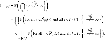
where (i) denotes the color string consisting of the color i only. Since the number of i-colored children (i.e. the number of children that are connected to r by an edge of color i) has distribution $\textrm{Poi}(\lambda_i)$
, its generating function is
$\textrm{Poi}(\lambda_i)$
, its generating function is $\exp({-}\lambda_i(1-z))$
for any
$\exp({-}\lambda_i(1-z))$
for any $i \in [k]$
. Thus we obtain
$i \in [k]$
. Thus we obtain
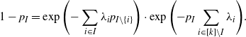 \begin{equation*} 1 - p_I = \exp\Bigg({-}\sum_{i \in I}\lambda_i p_{I \setminus \{i\}}\Bigg) \cdot \exp\Bigg({-}p_I\sum_{i \in [k] \setminus I}\lambda_i\Bigg). \end{equation*}
Let $k \in \mathbb{N}_+$
,
$k \in \mathbb{N}_+$
, $\underline{\lambda} \in \mathbb{R}_+^k$
, and consider the following system of equations:
$\underline{\lambda} \in \mathbb{R}_+^k$
, and consider the following system of equations:
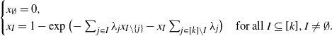 \begin{equation} \begin{cases} x_{\emptyset}=0, \\ x_I = 1 - \exp\big({-}\sum_{j \in I}\lambda_j x_{I \setminus \{j\}} - x_{I}\sum_{j \in [k] \setminus I}\lambda_j\big) & \textrm{for all}\ I \subseteq [k], I \neq \emptyset. \end{cases}\end{equation}
By Lemma 4.1, $(x_I)_{I \subseteq [k]} = (p_I)_{I \subseteq [k]}$
is a solution of this system, but note that this is not a unique solution, for instance
$(x_I)_{I \subseteq [k]} = (p_I)_{I \subseteq [k]}$
is a solution of this system, but note that this is not a unique solution, for instance $(x_I)_{I \subseteq [k]} = \underline{0}$
is also a solution.
$(x_I)_{I \subseteq [k]} = \underline{0}$
is also a solution.
Observe that if $\underline{x}^* = (x^*_I)_{I \subseteq [k]}$
is a solution to the system of equations (4.6), then
$\underline{x}^* = (x^*_I)_{I \subseteq [k]}$
is a solution to the system of equations (4.6), then $x^*_I < 1$
holds for any
$x^*_I < 1$
holds for any $I \subseteq [k]$
.
$I \subseteq [k]$
.
Definition 4.3. (Relevant solution.) We say that a solution $\underline{x}^*=(x^*_I)_{I \subseteq [k]}$
of the system of equations (4.6) is relevant if
$\underline{x}^*=(x^*_I)_{I \subseteq [k]}$
of the system of equations (4.6) is relevant if $0 < x^*_I < 1$
holds for any nonempty
$0 < x^*_I < 1$
holds for any nonempty $I \subseteq [k]$
. Otherwise
$I \subseteq [k]$
. Otherwise $\underline{x}^*$
is said to be irrelevant.
$\underline{x}^*$
is said to be irrelevant.
The next lemma gives a necessary and sufficient condition for $(p_I)_{I \subseteq [k]}$
to be a relevant solution.
$(p_I)_{I \subseteq [k]}$
to be a relevant solution.
Lemma 4.2. (The relevance of the probabilistic solution.) Let $k \in \mathbb{N}_+$
and
$k \in \mathbb{N}_+$
and $\underline{\lambda} \in \mathbb{R}_+^k$
. The probability vector
$\underline{\lambda} \in \mathbb{R}_+^k$
. The probability vector $(p_I)_{I \subseteq [k]}$
is a relevant solution of the system of equations (4.6) if and only if
$(p_I)_{I \subseteq [k]}$
is a relevant solution of the system of equations (4.6) if and only if $\underline{\lambda}$
is fully supercritical.
$\underline{\lambda}$
is fully supercritical.
Proof. Let $G_{\infty} \,:\!=\, G_{\infty}(r) \sim \mathcal{G}_{\infty}(\underline{\lambda})$
. First, assume that
$G_{\infty} \,:\!=\, G_{\infty}(r) \sim \mathcal{G}_{\infty}(\underline{\lambda})$
. First, assume that $\underline{\lambda}$
is fully supercritical. Then, for any nonempty
$\underline{\lambda}$
is fully supercritical. Then, for any nonempty $I \subseteq [k]$
,
$I \subseteq [k]$
,
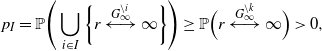 \begin{align*} p_I = \mathbb{P}\Bigg(\bigcup_{i \in I}\bigg\{r \stackrel{G_{\infty}^{\setminus i}}{\longleftrightarrow} \infty\bigg\}\Bigg) \ge \mathbb{P}\Big(r \stackrel{G_{\infty}^{\setminus k}}{\longleftrightarrow} \infty\Big) > 0, \end{align*}
and hence $(p_I)_{I \subseteq [k]}$
is indeed a relevant solution.
$(p_I)_{I \subseteq [k]}$
is indeed a relevant solution.
Now assume that $\underline{\lambda}$
is not fully supercritical, i.e. there exists a color
$\underline{\lambda}$
is not fully supercritical, i.e. there exists a color $i \in [k]$
such that
$i \in [k]$
such that $\lambda^{\setminus i} \le 1$
. Then
$\lambda^{\setminus i} \le 1$
. Then $p_{\{i\}} = \mathbb{P}\Big(r \stackrel{G_{\infty}^{\setminus i}}{\longleftrightarrow} \infty\Big) = 0$
, and thus
$p_{\{i\}} = \mathbb{P}\Big(r \stackrel{G_{\infty}^{\setminus i}}{\longleftrightarrow} \infty\Big) = 0$
, and thus $(p_I)_{I \subseteq [k]}$
is not a relevant solution.
$(p_I)_{I \subseteq [k]}$
is not a relevant solution.
Lemma 4.3. (Uniqueness of relevant solution.) Let $k \in \mathbb{N}_+$
and
$k \in \mathbb{N}_+$
and $\underline{\lambda} \in \mathbb{R}_+^k$
. If
$\underline{\lambda} \in \mathbb{R}_+^k$
. If $\underline{\lambda}$
is fully supercritical, then
$\underline{\lambda}$
is fully supercritical, then $(p_I)_{I \subseteq [k]}$
is a unique relevant solution of (4.6).
$(p_I)_{I \subseteq [k]}$
is a unique relevant solution of (4.6).
Proof. By the definition of a relevant solution, it is enough to show that
 \begin{equation} x_I = 1 - \exp\Bigg({-}\sum_{j \in I}\lambda_j p_{I \setminus \{j\}} - x_{I}\sum_{j \in [k] \setminus I}\lambda_j\Bigg) \end{equation}
has a unique solution in (0, 1), namely $p_I$
, for any nonempty
$p_I$
, for any nonempty $I \subseteq [k]$
. We prove this by induction on
$I \subseteq [k]$
. We prove this by induction on $|I|$
.
$|I|$
.
First, assume that $|I| = 1$
, i.e.
$|I| = 1$
, i.e. $I = \{i\}$
for some
$I = \{i\}$
for some $i \in [k]$
. Then we need to show that
$i \in [k]$
. Then we need to show that
 \begin{equation} x_{\{i\}} = 1 - \exp\Bigg({-}x_{\{i\}}\sum_{j \in [k] \setminus \{i\}}\lambda_j\Bigg). \end{equation}
Now, the left-hand side of (4.8) is linear in the variable $x_{\{ i \}}$
, while its right-hand side is exponential in
$x_{\{ i \}}$
, while its right-hand side is exponential in $x_{\{ i \}}$
, and it is well known that such equations have at most two solutions. As we saw earlier,
$x_{\{ i \}}$
, and it is well known that such equations have at most two solutions. As we saw earlier, $x_{\{ i \}} = 0$
and
$x_{\{ i \}} = 0$
and $x_{\{ i \}} = p_{\{ i \}}$
are both solutions, and by Lemma 4.2,
$x_{\{ i \}} = p_{\{ i \}}$
are both solutions, and by Lemma 4.2, $p_{\{ i \}} > 0$
. Thus, (4.8) indeed has a unique solution in (0, 1).
$p_{\{ i \}} > 0$
. Thus, (4.8) indeed has a unique solution in (0, 1).
Now let $I \subseteq [k]$
with
$I \subseteq [k]$
with $|I| \ge 2$
and assume that (4.7) holds for any
$|I| \ge 2$
and assume that (4.7) holds for any $I^{\prime} \subseteq [k]$
with
$I^{\prime} \subseteq [k]$
with $|I^{\prime}| < |I|$
. Consider first the case
$|I^{\prime}| < |I|$
. Consider first the case $I \ne [k]$
. Again, the left-hand side of (4.7) is linear, while its right-hand side is exponential in
$I \ne [k]$
. Again, the left-hand side of (4.7) is linear, while its right-hand side is exponential in $x_I$
, so there are at most two solutions. Clearly,
$x_I$
, so there are at most two solutions. Clearly, $p_{I}$
is a solution, and by Lemma 4.2, it is in (0, 1). In addition, in
$p_{I}$
is a solution, and by Lemma 4.2, it is in (0, 1). In addition, in $x_{I} = 0$
the left-hand side of (4.7) is clearly 0, while its right-hand side is
$x_{I} = 0$
the left-hand side of (4.7) is clearly 0, while its right-hand side is
 \begin{align*}1 - \exp\Bigg({-}\sum_{i \in I}\lambda_i p_{I \setminus \{i\}}\Bigg) > 1 - \textrm{e}^0 = 0,\end{align*}
so by the continuity of the linear and exponential functions, the other solution of (4.7) is negative.
Now consider the case $I = [k]$
. Then (4.7) becomes
$I = [k]$
. Then (4.7) becomes
 \begin{equation*} x_{[k]} = 1 - \exp\Bigg({-}\sum_{i \in [k]}\lambda_i p_{[k] \setminus \{i\}}\Bigg), \end{equation*}
which clearly has a unique solution. By Lemma 4.1, this solution is $p_I$
and it is in (0, 1).
$p_I$
and it is in (0, 1).
As is clear from the proof of Lemma 4.3, we should solve the equations of the system (4.6) in a nondecreasing order according to the size of their indices I. Using the Lambert W function (cf. (4.1)), we obtain the following.
Corollary 4.1. Let $k \in \mathbb{N}_+$
and
$k \in \mathbb{N}_+$
and $\underline{\lambda} \in \mathbb{R}_+^k$
. If
$\underline{\lambda} \in \mathbb{R}_+^k$
. If $\underline{\lambda}$
is fully supercritical, then
$\underline{\lambda}$
is fully supercritical, then
 \begin{equation*} p_{I} = 1 + \frac{W\big({-}\big(\sum_{i \in [k] \setminus I}\lambda_i\big) \exp\big({-}\sum_{i \in I}\lambda_i p_{I \setminus \{i\}} - \sum_{i \in [k] \setminus I}\lambda_i\big)\big)} {\sum_{i \in [k] \setminus I} \lambda_i} \end{equation*}
for any nonempty $I \subsetneq [k]$
, and
$I \subsetneq [k]$
, and $p_{[k]} = 1 - \exp\big({-}\sum_{i \in [k]}\lambda_i p_{[k] \setminus \{i\}}\big)$
.
$p_{[k]} = 1 - \exp\big({-}\sum_{i \in [k]}\lambda_i p_{[k] \setminus \{i\}}\big)$
.
Substituting these into (4.5), we get the required formula for $f^*_{\infty}$
. We note that using the values
$f^*_{\infty}$
. We note that using the values $p_I$
(and the help of computer software capable of symbolic computations), we can also prove the convergence statement of Theorem 2.1 in the case when
$p_I$
(and the help of computer software capable of symbolic computations), we can also prove the convergence statement of Theorem 2.1 in the case when $k \in \{ 2, 3, 4 \}$
and obtain the values
$k \in \{ 2, 3, 4 \}$
and obtain the values $C(2) = 4$
,
$C(2) = 4$
, $C(3) = 32$
, and
$C(3) = 32$
, and $C(4)=624$
, as stated in Theorem 2.1. Note that in Section 4.2 we introduce an alternative method with which the convergence statement of Theorem 2.1 can be proved for any integer
$C(4)=624$
, as stated in Theorem 2.1. Note that in Section 4.2 we introduce an alternative method with which the convergence statement of Theorem 2.1 can be proved for any integer $k\geq 2$
, and at the end of Section 4.2 we obtain the same values for C(k) when
$k\geq 2$
, and at the end of Section 4.2 we obtain the same values for C(k) when $k \in \{ 2, 3, 4 \}$
using this alternative approach.
$k \in \{ 2, 3, 4 \}$
using this alternative approach.
4.2. Using generating functions
The aim of this section is to give an explicit formula for $f^*_\infty$
and to prove Theorem 2.1. By Proposition 2.1, we can assume that the color intensity parameter vector
$f^*_\infty$
and to prove Theorem 2.1. By Proposition 2.1, we can assume that the color intensity parameter vector $\underline{\lambda} \in \mathbb{R}_+^k$
(where
$\underline{\lambda} \in \mathbb{R}_+^k$
(where $k \in \mathbb{N}_+$
) is fully supercritical. We also assume here that Assumption 2.1 holds for
$k \in \mathbb{N}_+$
) is fully supercritical. We also assume here that Assumption 2.1 holds for $\underline{\lambda}$
. Recall that this assumption heuristically means that we really need to use all of the other
$\underline{\lambda}$
. Recall that this assumption heuristically means that we really need to use all of the other $k-1$
colors to create an infinitely long i-avoiding path for each
$k-1$
colors to create an infinitely long i-avoiding path for each $i \in [k]$
.
$i \in [k]$
.
In order to find an explicit formula for $f^*_\infty$
, we first calculate the joint generating function of the random variables
$f^*_\infty$
, we first calculate the joint generating function of the random variables $\big|\widetilde{R}_{\underline{s}}(r)\big|$
,
$\big|\widetilde{R}_{\underline{s}}(r)\big|$
, $\underline{s} \in S_h$
, for any
$\underline{s} \in S_h$
, for any $h \in \{ 0, 1, \ldots, k-2\}$
. Note that, by Lemma 3.1,
$h \in \{ 0, 1, \ldots, k-2\}$
. Note that, by Lemma 3.1, $\Big( R_{\infty,d}^{\textrm{set}(\underline{s})} \Big)_{d \in \mathbb{N}}$
is a branching process with offspring distribution
$\Big( R_{\infty,d}^{\textrm{set}(\underline{s})} \Big)_{d \in \mathbb{N}}$
is a branching process with offspring distribution $\textrm{Poi}\big(\lambda_{\textrm{set}(\underline{s})}\big)$
.
$\textrm{Poi}\big(\lambda_{\textrm{set}(\underline{s})}\big)$
.
Definition 4.4 (Generating function of Borel distribution.) Let $k \in \mathbb{N}_+$
,
$k \in \mathbb{N}_+$
, $\underline{\lambda} \in \mathbb{R}_+^k$
,
$\underline{\lambda} \in \mathbb{R}_+^k$
, $G_{\infty} \,:\!=\, G_{\infty}(r) \sim \mathcal{G}_{\infty}(\underline{\lambda})$
,
$G_{\infty} \,:\!=\, G_{\infty}(r) \sim \mathcal{G}_{\infty}(\underline{\lambda})$
, $h \in \{ 0, 1, \ldots, k-1 \}$
, and let
$h \in \{ 0, 1, \ldots, k-1 \}$
, and let $\underline{s} \in S_h$
. We define
$\underline{s} \in S_h$
. We define $F_{\underline{s}} \colon [0,1) \to [0,1)$
such that
$F_{\underline{s}} \colon [0,1) \to [0,1)$
such that $z \mapsto \mathbb{E}\Big( z^{\big|\mathcal{C}\big(r, G_{\infty}^{\textrm{set}(\underline{s})}\big)\big|}\Big)$
, i.e. the generating function of the total number of individuals in the branching process
$z \mapsto \mathbb{E}\Big( z^{\big|\mathcal{C}\big(r, G_{\infty}^{\textrm{set}(\underline{s})}\big)\big|}\Big)$
, i.e. the generating function of the total number of individuals in the branching process $\Big( R_{\infty,d}^{\textrm{set}(\underline{s})} \Big)_{d \in \mathbb{N}}$
. We write
$\Big( R_{\infty,d}^{\textrm{set}(\underline{s})} \Big)_{d \in \mathbb{N}}$
. We write $F_{\underline{s}}(1_-) \,:\!=\, \lim_{z \to 1_-} F_{\underline{s}}(z)$
, i.e. the probability of the event that the branching process
$F_{\underline{s}}(1_-) \,:\!=\, \lim_{z \to 1_-} F_{\underline{s}}(z)$
, i.e. the probability of the event that the branching process $\Big( R_{\infty,d}^{\textrm{set}(\underline{s})} \Big)_{d \in \mathbb{N}}$
dies out.
$\Big( R_{\infty,d}^{\textrm{set}(\underline{s})} \Big)_{d \in \mathbb{N}}$
dies out.
Note that $F_{\underline{s}}$
can be expressed using the Lambert W function as
$F_{\underline{s}}$
can be expressed using the Lambert W function as
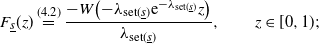 \begin{equation} F_{\underline{s}}(z) \stackrel{({4.2})}{=} \frac{-W\big({-}\lambda_{\textrm{set}(\underline{s})}\textrm{e}^{-\lambda_{\textrm{set}(\underline{s})}}z\big)} {\lambda_{\textrm{set}(\underline{s})}}, \qquad z \in [0,1);\end{equation}
that if $\textrm{set}(\underline{s}) = \textrm{set}(\underline{s}^{\prime})$
holds for some color strings
$\textrm{set}(\underline{s}) = \textrm{set}(\underline{s}^{\prime})$
holds for some color strings $\underline{s}, \underline{s}^{\prime} \in S_h$
with
$\underline{s}, \underline{s}^{\prime} \in S_h$
with $h \in \{ 0, 1, \ldots, k-2 \}$
then
$h \in \{ 0, 1, \ldots, k-2 \}$
then $F_{\underline{s}} \equiv F^{\prime}_{\underline{s}}$
; and that if
$F_{\underline{s}} \equiv F^{\prime}_{\underline{s}}$
; and that if $\underline{\lambda}$
is fully supercritical and Assumption 2.1 holds, then
$\underline{\lambda}$
is fully supercritical and Assumption 2.1 holds, then $F_{\underline{s}}(1_-) = 1$
for any
$F_{\underline{s}}(1_-) = 1$
for any $\underline{s} \in S_h$
with
$\underline{s} \in S_h$
with $h \in \{ 0, 1, \ldots, k-2 \}$
, and
$h \in \{ 0, 1, \ldots, k-2 \}$
, and $F_{\underline{s}}(1_-) < 1$
for any
$F_{\underline{s}}(1_-) < 1$
for any $\underline{s} \in S_{k-1}$
.
$\underline{s} \in S_{k-1}$
.
Definition 4.5. (Joint generating function of the number of vertices reachable by different color chronologies in an ECBP tree.) Let $k \in \mathbb{N}_+$
,
$k \in \mathbb{N}_+$
, $\underline{\lambda} \in \mathbb{R}_+^k$
,
$\underline{\lambda} \in \mathbb{R}_+^k$
, $G_{\infty}(r) \sim \mathcal{G}_{\infty}(\underline{\lambda})$
, and
$G_{\infty}(r) \sim \mathcal{G}_{\infty}(\underline{\lambda})$
, and $h \in \{ 0, 1, \ldots,$ $k-2 \}$
. We define
$k-2 \}$
. We define $\Phi_h\colon [0,1)^{S_h} \to [0,1)$
such that
$\Phi_h\colon [0,1)^{S_h} \to [0,1)$
such that
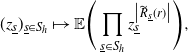 \begin{align*} (z_{\underline{s}})_{\underline{s} \in S_h} \mapsto \mathbb{E}\Bigg(\prod_{\underline{s} \in S_h}z_{\underline{s}}^{\big|\widetilde{R}_{\underline{s}}(r)\big|}\Bigg), \end{align*}
and write $\Phi_h\big((1_-)_{\underline{s} \in S_h}\big) \,:\!=\, \lim_{\{\textrm{for all}\ \underline{s} \in S_h\colon z_{\underline{s}} \to 1_-\}}\Phi_h\big((z_{\underline{s}})_{\underline{s}\in S_h}\big)$
.
$\Phi_h\big((1_-)_{\underline{s} \in S_h}\big) \,:\!=\, \lim_{\{\textrm{for all}\ \underline{s} \in S_h\colon z_{\underline{s}} \to 1_-\}}\Phi_h\big((z_{\underline{s}})_{\underline{s}\in S_h}\big)$
.
It follows from the definition of $S_0$
(cf. Definition 3.1) that
$S_0$
(cf. Definition 3.1) that $\Phi_0(z) = z$
. Note that if Assumption 2.1 holds, then
$\Phi_0(z) = z$
. Note that if Assumption 2.1 holds, then $\mathbb{P}\big(\big|\widetilde{R}_{\underline{s}}(r)\big| < +\infty\big) = 1$
for any
$\mathbb{P}\big(\big|\widetilde{R}_{\underline{s}}(r)\big| < +\infty\big) = 1$
for any $\underline{s} \in S_h$
with
$\underline{s} \in S_h$
with $h \in \{ 0, 1, \ldots, k-2 \}$
. Therefore,
$h \in \{ 0, 1, \ldots, k-2 \}$
. Therefore, $\Phi_h\big((1_-)_{\underline{s} \in S_h}\big) = 1$
for any
$\Phi_h\big((1_-)_{\underline{s} \in S_h}\big) = 1$
for any $h \in \{ 0, 1, \ldots, k-2 \}$
.
$h \in \{ 0, 1, \ldots, k-2 \}$
.
Now we give a recursive formula for $\Phi_{h+1}$
in terms of
$\Phi_{h+1}$
in terms of $\Phi_h$
for any
$\Phi_h$
for any $h \in \{ 0, 1, \ldots, k-3 \}$
. Note that this formula can be viewed as ‘explicit’ since it can be written as a composition of elementary functions and the Lambert W function (cf. (4.9)).
$h \in \{ 0, 1, \ldots, k-3 \}$
. Note that this formula can be viewed as ‘explicit’ since it can be written as a composition of elementary functions and the Lambert W function (cf. (4.9)).
Lemma 4.4. (Recursion for the joint generating function of the number of vertices reachable by different color chronologies.) Let $k \in \mathbb{N}_+$
,
$k \in \mathbb{N}_+$
, $\underline{\lambda} \in \mathbb{R}_+^k$
, and
$\underline{\lambda} \in \mathbb{R}_+^k$
, and $G_{\infty}(r) \sim \mathcal{G}_{\infty}(\underline{\lambda})$
. Then, for any
$G_{\infty}(r) \sim \mathcal{G}_{\infty}(\underline{\lambda})$
. Then, for any $h \in \{ 0, 1, \ldots, k-3 \}$
,
$h \in \{ 0, 1, \ldots, k-3 \}$
,
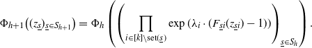 \begin{align*} \Phi_{h+1}\big((z_{\underline{s}})_{\underline{s} \in S_{h+1}}\big) = \Phi_h\left(\left(\prod_{i \in [k] \setminus \textrm{set}(\underline{s})} \exp(\lambda_i \cdot (F_{\underline{s}i}(z_{\underline{s}i})-1))\right)_{\underline{s} \in S_h}\right). \end{align*}
In words, we have to plug $\prod_{i \in [k] \setminus \textrm{set}(\underline{s})}\exp\big(\lambda_i\cdot\big(F_{\underline{s}i}(z_{\underline{s}i})-1\big)\big)$
in place of the variable
$\prod_{i \in [k] \setminus \textrm{set}(\underline{s})}\exp\big(\lambda_i\cdot\big(F_{\underline{s}i}(z_{\underline{s}i})-1\big)\big)$
in place of the variable $z_{\underline{s}}$
for every
$z_{\underline{s}}$
for every $\underline{s} \in S_h$
in the function
$\underline{s} \in S_h$
in the function $\Phi_h \big( (z_{\underline{s}})_{\underline{s} \in S_h} \big)$
.
$\Phi_h \big( (z_{\underline{s}})_{\underline{s} \in S_h} \big)$
.
Proof of Lemma
4.4. First, note that each color string of length $h+1$
can be uniquely written as the concatenation of a color string of length h and a color not appearing in this color string. Therefore, by the tower rule,
$h+1$
can be uniquely written as the concatenation of a color string of length h and a color not appearing in this color string. Therefore, by the tower rule,
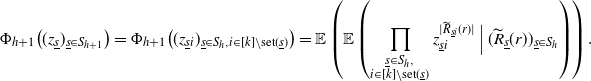 \begin{equation*} \Phi_{h+1}\big((z_{\underline{s}})_{\underline{s} \in S_{h+1}}\big) = \Phi_{h+1}\big((z_{\underline{s}i})_{\underline{s} \in S_h, i \in [k] \setminus \textrm{set}(\underline{s})}\big) = \mathbb{E}\left(\mathbb{E}\left( \prod_{\substack{\underline{s}\in S_h,\\i\in[k]\setminus\textrm{set}(\underline{s})}}z_{\underline{s}i}^{|\widetilde{R}_{\underline{s}i}(r)|} \,\Big|\, (\widetilde{R}_{\underline{s}}(r))_{\underline{s} \in S_h}\right)\right). \end{equation*}
By the independence of the different branches of an ECBP tree,
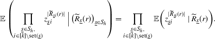 \begin{align*} \mathbb{E}\left(\prod_{\substack{\underline{s} \in S_h, \\ i \in [k] \setminus \textrm{set}(\underline{s})}} z_{\underline{s}i}^{|\widetilde{R}_{\underline{s}i}(r)|} \,\Big|\, \big(\widetilde{R}_{\underline{s}}(r)\big)_{\underline{s}\in S_h}\right) = \prod_{\substack{\underline{s} \in S_h, \\ i \in [k] \setminus \textrm{set}(\underline{s})}} \mathbb{E}\bigg(z_{\underline{s}i}^{|\widetilde{R}_{\underline{s}i}(r)|} \mid \widetilde{R}_{\underline{s}}(r)\bigg). \end{align*}
Let $\underline{s} \in S_h$
and
$\underline{s} \in S_h$
and $i \in [k] \setminus \textrm{set}(\underline{s})$
. Using that for any
$i \in [k] \setminus \textrm{set}(\underline{s})$
. Using that for any $v \in \widetilde{R}_{\underline{s}}(r)$
, the function
$v \in \widetilde{R}_{\underline{s}}(r)$
, the function $z \mapsto \exp(\lambda_i \cdot (F_{\underline{s}i}(z) - 1))$
is the generating function of the cardinality of the set of descendants of v belonging to
$z \mapsto \exp(\lambda_i \cdot (F_{\underline{s}i}(z) - 1))$
is the generating function of the cardinality of the set of descendants of v belonging to $\widetilde{R}_{\underline{s}i}(r)$
, we obtain
$\widetilde{R}_{\underline{s}i}(r)$
, we obtain
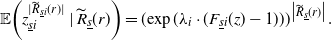 \begin{align*} \mathbb{E}\bigg(z_{\underline{s}i}^{|\widetilde{R}_{\underline{s}i}(r)|} \mid \widetilde{R}_{\underline{s}}(r)\bigg) = (\!\exp(\lambda_i \cdot (F_{\underline{s}i}(z) - 1)))^{\big|\widetilde{R}_{\underline{s}}(r)\big|}. \end{align*}
Therefore, and by the definition of the function $\Phi_h$
, we obtain
$\Phi_h$
, we obtain
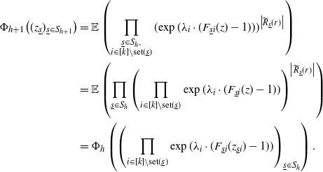 \begin{align*} \Phi_{h+1}\big((z_{\underline{s}})_{\underline{s} \in S_{h+1}}\big) & = \mathbb{E}\left(\prod_{\substack{\underline{s} \in S_h, \\ i \in [k] \setminus \textrm{set}(\underline{s})}} (\!\exp(\lambda_i \cdot (F_{\underline{s}i}(z) - 1)))^{\big|\widetilde{R}_{\underline{s}}(r)\big|}\right) \\ & = \mathbb{E}\left(\prod_{\underline{s} \in S_h}\left(\prod_{i \in [k] \setminus \textrm{set}(\underline{s})} \exp(\lambda_i \cdot (F_{\underline{s}i}(z) - 1))\right)^{\big|\widetilde{R}_{\underline{s}}(r)\big|}\right) \\ & = \Phi_h\left(\left(\prod_{i \in [k] \setminus \textrm{set}(\underline{s})} \exp(\lambda_i \cdot (F_{\underline{s}i}(z_{\underline{s}i}) - 1))\right)_{\underline{s} \in S_h}\right). \end{align*}
Definition 4.6. (Color strings of length $k-1$
avoiding color i.) Let
$k-1$
avoiding color i.) Let $k \in \mathbb{N}_+$
. For any
$k \in \mathbb{N}_+$
. For any $i \in [k]$
, let
$i \in [k]$
, let $S_{k-1}^{\setminus i} \,:\!=\, \{ \underline{s} \in S_{k-1} \colon \textrm{set}(\underline{s}) = [k] \setminus \{i\}\}$
.
$S_{k-1}^{\setminus i} \,:\!=\, \{ \underline{s} \in S_{k-1} \colon \textrm{set}(\underline{s}) = [k] \setminus \{i\}\}$
.
Proposition 4.1. (Explicit formula for $f^*_\infty$
.) Let
$f^*_\infty$
.) Let $k \in \mathbb{N}_+$
, let
$k \in \mathbb{N}_+$
, let $\underline{\lambda} \in \mathbb{R}^k_+$
for which Assumption 2.1 holds, and let
$\underline{\lambda} \in \mathbb{R}^k_+$
for which Assumption 2.1 holds, and let $G_{\infty} \,:\!=\, G_{\infty}(r) \sim \mathcal{G}_{\infty}(\underline{\lambda})$
. Then
$G_{\infty} \,:\!=\, G_{\infty}(r) \sim \mathcal{G}_{\infty}(\underline{\lambda})$
. Then
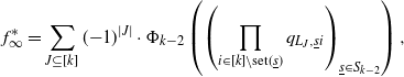 \begin{align*} f^*_\infty = \sum_{J \subseteq [k]}({-}1)^{|J|} \cdot \Phi_{k-2}\left(\left( \prod_{i \in [k] \setminus \textrm{set}(\underline{s})}q_{L_J,\underline{s}i}\right)_{\underline{s} \in S_{k-2}}\right), \end{align*}
where we define $L_J \,:\!=\, \bigcup_{j \in J} S_{k-1}^{\setminus j}$
,
$L_J \,:\!=\, \bigcup_{j \in J} S_{k-1}^{\setminus j}$
, $J \subseteq [k]$
, and we define, for any
$J \subseteq [k]$
, and we define, for any $L \subseteq S_{k-1}$
,
$L \subseteq S_{k-1}$
, $\underline{s} \in S_{k-2}$
, and
$\underline{s} \in S_{k-2}$
, and $i \in [k] \setminus \textrm{set}(\underline{s})$
,
$i \in [k] \setminus \textrm{set}(\underline{s})$
,
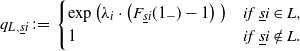 \begin{align*} q_{L,\underline{s}i} \,:\!=\, \begin{cases} \exp\big(\lambda_i \cdot \left(F_{\underline{s}i}(1_-) - 1\right)\big) & if\ \underline{s}i \in L, \\ 1 & if\ \underline{s}i \notin L. \end{cases} \end{align*}
Proof. If $v \in V(G_\infty)$
and
$v \in V(G_\infty)$
and $i \in [k]$
, let us denote by
$i \in [k]$
, let us denote by $\widetilde{N}^*_{(i)}(v)$
the set of children of v that are connected to v by an edge of color i. Let
$\widetilde{N}^*_{(i)}(v)$
the set of children of v that are connected to v by an edge of color i. Let $\mathcal{F}$
denote the sigma-algebra
$\mathcal{F}$
denote the sigma-algebra
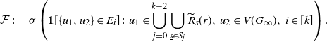 \begin{align*} \mathcal{F} \,:\!=\, \sigma\left(\textbf{1}[\{u_1, u_2\} \in E_i] \colon u_1 \in \bigcup_{j=0}^{k-2}\bigcup_{\underline{s} \in S_j}\widetilde{R}_{\underline{s}}(r),\; u_2 \in V(G_\infty), \; i \in [k]\right). \end{align*}
In words: $\mathcal{F}$
contains the information that we collect if we explore the set of vertices of
$\mathcal{F}$
contains the information that we collect if we explore the set of vertices of $G_\infty$
that can be reached by a path from the root that uses at most
$G_\infty$
that can be reached by a path from the root that uses at most $k-2$
colors, and all edges emanating from this set. Assumption 2.1 implies that this set is almost surely finite.
$k-2$
colors, and all edges emanating from this set. Assumption 2.1 implies that this set is almost surely finite.
By Lemma 3.1 and using that each offspring of any vertex in a branching process tree spans a branching process tree with the same offspring distribution, and by the definition of $\Phi_{k-2}$
, for any
$\Phi_{k-2}$
, for any $L \subseteq S_{k-1}$
, we obtain
$L \subseteq S_{k-1}$
, we obtain
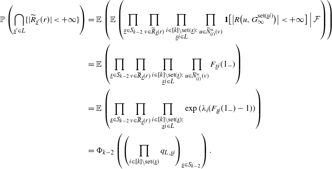 \begin{align} \mathbb{P}\left(\bigcap_{\underline{s}^{\prime} \in L}\{|\widetilde{R}_{\underline{s}^{\prime}}(r)| < +\infty\}\right) & = \mathbb{E}\left(\mathbb{E}\left(\prod_{\underline{s} \in S_{k-2}}\prod_{v \in \widetilde{R}_{\underline{s}}(r)} \prod_{\substack{i \in [k] \setminus \textrm{set}(\underline{s}): \\ \underline{s}i \in L}}\prod_{u \in \widetilde{N}^*_{(i)}(v)} \textbf{1}\big[\big|R\big(u,G_{\infty}^{\textrm{set}(\underline{s}i)}\big)\big| < +\infty\big] \,\Big|\, \mathcal{F}\right)\right) \nonumber \\ & = \mathbb{E}\left(\prod_{\underline{s} \in S_{k-2}}\prod_{v \in \widetilde{R}_{\underline{s}}(r)} \prod_{\substack{i \in [k] \setminus \textrm{set}(\underline{s}): \\ \underline{s}i \in L}}\prod_{u \in \widetilde{N}^*_{(i)}(v)} F_{\underline{s}i}(1_-)\right) \nonumber \\ & = \mathbb{E}\left(\prod_{\underline{s} \in S_{k-2}}\prod_{v \in \widetilde{R}_{\underline{s}}(r)} \prod_{\substack{i \in [k] \setminus \textrm{set}(\underline{s}): \\ \underline{s}i \in L}} \exp(\lambda_i(F_{\underline{s}i}(1_-) - 1))\right) \nonumber \\ & = \Phi_{k-2}\left(\left(\prod_{i \in [k] \setminus \textrm{set}(\underline{s})} q_{L,\underline{s}i}\right)_{\underline{s} \in S_{k-2}}\right). \end{align}
By the definition of $\widetilde{R}_{\underline{s}}(r)$
(cf. Definition 3.3) we have
$\widetilde{R}_{\underline{s}}(r)$
(cf. Definition 3.3) we have
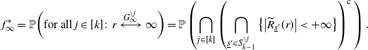 \begin{align*} f^*_\infty = \mathbb{P}\bigg(\textrm{for all}\ j \in [k] \colon r \stackrel{G_{\infty}^{\setminus j} }{\longleftrightarrow} \infty\bigg) = \mathbb{P}\left(\bigcap_{j \in [k]}\left(\bigcap_{\underline{s}^{\prime} \in S_{k-1}^{\setminus j}} \big\{\big|\widetilde{R}_{\underline{s}^{\prime}}(r)\big| < +\infty\big\}\right)^\textrm{c}\,\right). \end{align*}
Then, by the inclusion–exclusion formula, the definition of $L_J$
, and (4.10), the previous equation implies
$L_J$
, and (4.10), the previous equation implies
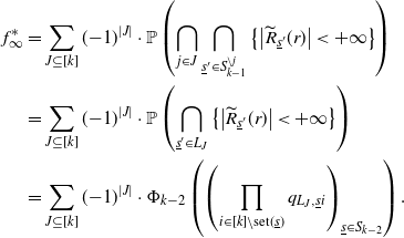 \begin{align*} f^*_\infty & = \sum_{J \subseteq [k]}({-}1)^{|J|} \cdot \mathbb{P}\left(\bigcap_{j \in J}\bigcap_{\underline{s}^{\prime} \in S_{k-1}^{\setminus j}} \big\{\big|\widetilde{R}_{\underline{s}^{\prime}}(r)\big| < +\infty\big\}\right) \\ & = \sum_{J \subseteq [k]}({-}1)^{|J|} \cdot \mathbb{P}\left(\bigcap_{\underline{s}^{\prime} \in L_J} \big\{\big|\widetilde{R}_{\underline{s}^{\prime}}(r)\big| < +\infty\big\}\right) \\ & = \sum_{J \subseteq [k]}({-}1)^{|J|} \cdot \Phi_{k-2}\left(\left(\prod_{i \in [k] \setminus \textrm{set}(\underline{s})} q_{L_J,\underline{s}i}\right)_{\underline{s} \in S_{k-2}}\right). \end{align*}
Proof of Theorem
2.1. Let $\varepsilon \ge 0$
and let
$\varepsilon \ge 0$
and let $G_{\infty}^{\varepsilon} \,:\!=\, G_{\infty}^{\varepsilon}(r) \sim \mathcal{G}_{\infty}(\underline{\lambda}(\varepsilon))$
, where
$G_{\infty}^{\varepsilon} \,:\!=\, G_{\infty}^{\varepsilon}(r) \sim \mathcal{G}_{\infty}(\underline{\lambda}(\varepsilon))$
, where
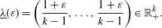 \begin{align*} \underline{\lambda}(\varepsilon) = \bigg(\frac{1+\varepsilon}{k-1},\ldots,\frac{1+\varepsilon}{k-1}\bigg) \in \mathbb{R}_+^k. \end{align*}
Since $\underline{\lambda}(\varepsilon)$
is homogeneous,
$\underline{\lambda}(\varepsilon)$
is homogeneous, $\theta^{\setminus k}(\varepsilon) \,:\!=\, \mathbb{P}\Big(r \stackrel{(G_{\infty}^{\varepsilon})^{\setminus k}}\leftrightarrow \infty\Big) = \mathbb{P}\Big(r \stackrel{{(G_{\infty}^{\varepsilon})^{\setminus i}}}\leftrightarrow \infty\Big)$
holds for any
$\theta^{\setminus k}(\varepsilon) \,:\!=\, \mathbb{P}\Big(r \stackrel{(G_{\infty}^{\varepsilon})^{\setminus k}}\leftrightarrow \infty\Big) = \mathbb{P}\Big(r \stackrel{{(G_{\infty}^{\varepsilon})^{\setminus i}}}\leftrightarrow \infty\Big)$
holds for any $i \in [k]$
.
$i \in [k]$
.
Note that if $\varepsilon < {1}/({k-2})$
then Assumption 2.1 holds, which implies that
$\varepsilon < {1}/({k-2})$
then Assumption 2.1 holds, which implies that $\bigcup_{j=0}^{k-2} \bigcup_{\underline{s} \in S_j}\!\widetilde{R}_{\underline{s}}(r)$
is almost surely finite (cf. Definition 3.3), and thus every i-avoiding path from r to infinity must pass through
$\bigcup_{j=0}^{k-2} \bigcup_{\underline{s} \in S_j}\!\widetilde{R}_{\underline{s}}(r)$
is almost surely finite (cf. Definition 3.3), and thus every i-avoiding path from r to infinity must pass through $\widetilde{N}_{k-1}^{\setminus i} (r)$
(cf. Definition 3.3); we therefore have
$\widetilde{N}_{k-1}^{\setminus i} (r)$
(cf. Definition 3.3); we therefore have
 \begin{align*} f^*_{\infty}(\varepsilon) = \mathbb{P}\bigg(\textrm{for all}\ i \in [k]\ \textrm{there exists}\ v \in \widetilde{N}_{k-1}^{\setminus i}\big(r, G_{\infty}^{\varepsilon}\big) \colon v\stackrel{{(G_{\infty}^{\varepsilon})^{\setminus i}}}\leftrightarrow \infty\bigg). \end{align*}
So, by (4.3) and the disjointness of the sets $\widetilde{N}_{k-1}^{\setminus i}\big(r, G_{\infty}^{\varepsilon}\big)$
for all
$\widetilde{N}_{k-1}^{\setminus i}\big(r, G_{\infty}^{\varepsilon}\big)$
for all $i \in [k]$
, the previous equation implies that
$i \in [k]$
, the previous equation implies that
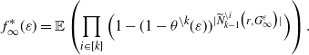 \begin{equation} f^*_{\infty}(\varepsilon) = \mathbb{E}\left(\prod_{i \in [k]}\Big(1 - (1 - \theta^{\setminus k}(\varepsilon))^{|\widetilde{N}_{k-1}^{\setminus i}\big(r, G_{\infty}^{\varepsilon}\big)|}\Big)\right). \end{equation}
Clearly, $\lambda^{\setminus k}(\varepsilon) \,:\!=\, \sum_{i \in [k-1]}\lambda_i(\varepsilon) = 1 + \varepsilon$
holds, and thus by [Reference Van der Hofstad31, Corollary 3.19] we have
$\lambda^{\setminus k}(\varepsilon) \,:\!=\, \sum_{i \in [k-1]}\lambda_i(\varepsilon) = 1 + \varepsilon$
holds, and thus by [Reference Van der Hofstad31, Corollary 3.19] we have $\lim_{\varepsilon \to 0_+}{\theta^{\setminus k}(\varepsilon)}/{\varepsilon} = 2$
. Hence,
$\lim_{\varepsilon \to 0_+}{\theta^{\setminus k}(\varepsilon)}/{\varepsilon} = 2$
. Hence,
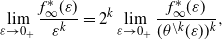 \begin{equation} \lim_{\varepsilon \to 0_+}\frac{f^*_{\infty}(\varepsilon)}{\varepsilon^k} = 2^k\lim_{\varepsilon \to 0_+}\frac{f^*_{\infty}(\varepsilon)}{(\theta^{\setminus k}(\varepsilon))^k}, \end{equation}
and now we show that
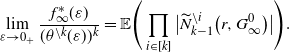 \begin{equation} \lim_{\varepsilon \to 0_+}\frac{f^*_{\infty}(\varepsilon)}{(\theta^{\setminus k}(\varepsilon))^k} = \mathbb{E}\Bigg(\prod_{i \in [k]}\big|\widetilde{N}_{k-1}^{\setminus i}\big(r, G_{\infty}^0\big)\big|\Bigg). \end{equation}
By Assumption 2.1, there exists $\varepsilon_0 \ge 0$
such that
$\varepsilon_0 \ge 0$
such that
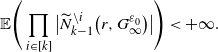 \begin{equation} \mathbb{E}\Bigg(\prod_{i \in [k]}\big|\widetilde{N}_{k-1}^{\setminus i}\big(r, G_{\infty}^{\varepsilon_0}\big)\big|\Bigg) < +\infty. \end{equation}
Then, by the monotone coupling of the random variables $\big|\widetilde{N}_{k-1}^{\setminus i}\big(r, G_{\infty}^{\varepsilon}\big)\big|$
for all
$\big|\widetilde{N}_{k-1}^{\setminus i}\big(r, G_{\infty}^{\varepsilon}\big)\big|$
for all $\varepsilon \in [0, \varepsilon_0]$
, and by Bernoulli’s inequality, we obtain
$\varepsilon \in [0, \varepsilon_0]$
, and by Bernoulli’s inequality, we obtain
 \begin{equation} \prod_{i \in [k]}\bigg(1 - (1 - \theta^{\setminus k}(\varepsilon))^{\big|\widetilde{N}_{k-1}^{\setminus i}\big(r, G_{\infty}^{\varepsilon}\big)\big|}\bigg) \le \prod_{i \in [k]}\big|\widetilde{N}_{k-1}^{\setminus i}\big(r, G_{\infty}^{\varepsilon}\big)\big| \le \prod_{i \in [k]}\big|\widetilde{N}_{k-1}^{\setminus i}\big(r, G_{\infty}^{\varepsilon_0}\big)\big|. \end{equation}
By (4.14) and (4.15), we may apply the dominated convergence theorem (using the random variable that appears on the right-hand side of (4.15) as the dominating random variable) to conclude that the first equality below holds. Then we can calculate (using L’Hospital’s rule in the last equality):
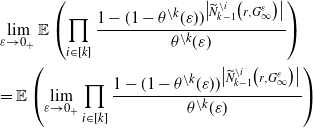 \begin{align*} & \lim_{\varepsilon \to 0_+}\mathbb{E}\left(\prod_{i \in [k]} \frac{1 - (1 - \theta^{\setminus k}(\varepsilon))^{\big|\widetilde{N}_{k-1}^{\setminus i}\big(r, G_{\infty}^{\varepsilon}\big)\big|}} {\theta^{\setminus k}(\varepsilon)}\right) \\ & = \mathbb{E}\left(\lim_{\varepsilon \to 0_+}\prod_{i \in [k]} \frac{1 - (1 - \theta^{\setminus k}(\varepsilon))^{\big|\widetilde{N}_{k-1}^{\setminus i}\big(r, G_{\infty}^{\varepsilon}\big)\big|}} {\theta^{\setminus k}(\varepsilon)}\right)\end{align*}
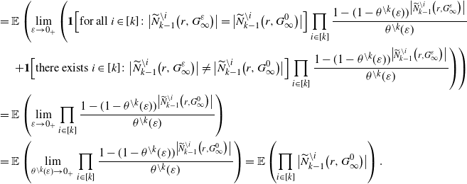 \begin{align*} & = \mathbb{E}\left(\lim_{\varepsilon \to 0_+}\left( \textbf{1}\Big[\textrm{for all}\ i \in [k] \colon \big|\widetilde{N}_{k-1}^{\setminus i}\big(r, G_{\infty}^{\varepsilon}\big)\big| = \big|\widetilde{N}_{k-1}^{\setminus i}\big(r, G_{\infty}^0\big)\big|\Big]\prod_{i \in [k]} \frac{1 - (1 - \theta^{\setminus k}(\varepsilon))^{\big|\widetilde{N}_{k-1}^{\setminus i}\big(r, G_{\infty}^{\varepsilon}\big)\big|}} {\theta^{\setminus k}(\varepsilon)} \right.\right.\\ & \left.\left. \quad + \textbf{1}\Big[\textrm{there exists}\ i \in [k] \colon \big|\widetilde{N}_{k-1}^{\setminus i}\big(r, G_{\infty}^{\varepsilon}\big)\big| \ne \big|\widetilde{N}_{k-1}^{\setminus i}\big(r, G_{\infty}^0\big)\big|\Big]\prod_{i \in [k]} \frac{1 - (1 - \theta^{\setminus k}(\varepsilon))^{\big|\widetilde{N}_{k-1}^{\setminus i}\big(r, G_{\infty}^{\varepsilon}\big)\big|}} {\theta^{\setminus k}(\varepsilon)}\right)\right)\\ & = \mathbb{E}\left(\lim_{\varepsilon \to 0_+}\prod_{i \in [k]} \frac{1 - (1 - \theta^{\setminus k}(\varepsilon))^{\big|\widetilde{N}_{k-1}^{\setminus i}\big(r, G_{\infty}^0\big)\big|}} {\theta^{\setminus k}(\varepsilon)}\right) \\ & = \mathbb{E}\left(\lim_{\theta^{\setminus k}(\varepsilon) \to 0_+}\prod_{i \in [k]} \frac{1 - (1 - \theta^{\setminus k}(\varepsilon))^{\big|\widetilde{N}_{k-1}^{\setminus i}\big(r, G_{\infty}^0\big)\big|}} {\theta^{\setminus k}(\varepsilon)}\right) = \mathbb{E}\left(\prod_{i \in [k]}\big|\widetilde{N}_{k-1}^{\setminus i}\big(r, G_{\infty}^0\big)\big|\right). \end{align*}
Thus, by (4.11), we obtain that (4.13) holds. Therefore, by (4.12), we obtain
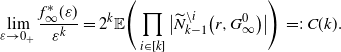 \begin{align*} \lim_{\varepsilon \to 0_+}\frac{f^*_{\infty}(\varepsilon)}{\varepsilon^k} = 2^k\mathbb{E}\Bigg(\prod_{i \in [k]}\big|\widetilde{N}_{k-1}^{\setminus i}\big(r, G_{\infty}^0\big)\big|\Bigg) \,=\!:\, C(k). \end{align*}
Now we want to express this constant C(k) using the generating function $\Phi_{k-2}$
, where we take the underlying parameter
$\Phi_{k-2}$
, where we take the underlying parameter $\underline{\lambda}$
to be
$\underline{\lambda}$
to be
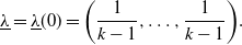 \begin{align*} \underline{\lambda} = \underline{\lambda}(0) = \bigg( \frac{1}{k-1}, \ldots, \frac{1}{k-1} \bigg). \end{align*}
Since the sets $\widetilde{N}_{\underline{s}}\big(r, G_{\infty}^0\big)$
for all
$\widetilde{N}_{\underline{s}}\big(r, G_{\infty}^0\big)$
for all $\underline{s} \in S_{k-1}$
are disjoint, it follows that
$\underline{s} \in S_{k-1}$
are disjoint, it follows that
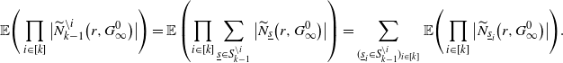 \begin{equation*} \mathbb{E}\Bigg(\prod_{i \in [k]}\big|\widetilde{N}_{k-1}^{\setminus i}\big(r, G_{\infty}^0\big)\big|\Bigg) = \mathbb{E}\left(\prod_{i \in [k]}\sum_{\underline{s} \in S_{k-1}^{\setminus i}} \big|\widetilde{N}_{\underline{s}}\big(r, G_{\infty}^0\big)\big|\right) = \sum_{(\underline{s}_i \in S_{k-1}^{\setminus i})_{i \in [k]}} \mathbb{E}\Bigg(\prod_{i \in [k]}\big|\widetilde{N}_{\underline{s}_i}\big(r, G_{\infty}^0\big)\big|\Bigg). \end{equation*}
Let $\underline{s}_i \in S_{k-1}^{\setminus i}$
for all
$\underline{s}_i \in S_{k-1}^{\setminus i}$
for all $i \in [k]$
. Since the random variables
$i \in [k]$
. Since the random variables $\big|\widetilde{N}_{\underline{s}_i}\big(r, G_{\infty}^0\big)\big|$
for all
$\big|\widetilde{N}_{\underline{s}_i}\big(r, G_{\infty}^0\big)\big|$
for all $i \in [k]$
are conditionally independent given
$i \in [k]$
are conditionally independent given $\big(\big|\widetilde{R}_{\underline{s}}\big(r, G_{\infty}^0\big)\big|\big)_{\underline{s} \in S_{k-2}}$
, and their conditional distribution is Poisson with parameter
$\big(\big|\widetilde{R}_{\underline{s}}\big(r, G_{\infty}^0\big)\big|\big)_{\underline{s} \in S_{k-2}}$
, and their conditional distribution is Poisson with parameter $\big|\widetilde{R}_{\underline{s}}\big(r, G_{\infty}^0\big)\big|/(k-1)$
, we obtain
$\big|\widetilde{R}_{\underline{s}}\big(r, G_{\infty}^0\big)\big|/(k-1)$
, we obtain
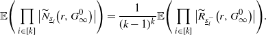 \begin{align*} \mathbb{E}\Bigg(\prod_{i \in [k]}\big|\widetilde{N}_{\underline{s}_i}\big(r, G_{\infty}^0\big)\big|\Bigg) = \frac{1}{(k-1)^k}\mathbb{E}\Bigg(\prod_{i \in [k]}\big|\widetilde{R}_{\underline{s}_i^-}\big(r, G_{\infty}^0\big)\big|\Bigg). \end{align*}
Let us define the multivariate moment-generating function
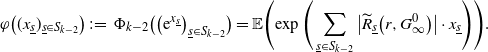 \begin{align*} \varphi\big((x_{\underline{s}})_{\underline{s} \in S_{k-2}}\big) \,:\!=\, \Phi_{k-2}\big(\big(\textrm{e}^{x_{\underline{s}}}\big)_{\underline{s} \in S_{k-2}}\big) = \mathbb{E}\Bigg(\!\exp\Bigg(\sum_{\underline{s} \in S_{k-2}}\big|\widetilde{R}_{\underline{s}}\big(r, G_{\infty}^0\big)\big| \cdot x_{\underline{s}}\Bigg)\Bigg). \end{align*}
Since the function $\varphi$
is the multivariate moment-generating function of the random vector
$\varphi$
is the multivariate moment-generating function of the random vector $\big(\big|\widetilde{R}_{\underline{s}}\big(r, G_{\infty}^0\big)\big|\big)_{\underline{s} \in S_{k-2}}$
, we obtain
$\big(\big|\widetilde{R}_{\underline{s}}\big(r, G_{\infty}^0\big)\big|\big)_{\underline{s} \in S_{k-2}}$
, we obtain
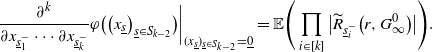 \begin{align*} \frac{\partial^k}{\partial x_{{\underline{s}_1^-}} \cdots \partial x_{{\underline{s}_k^-}}} \varphi\big(\big(x_{\underline{s}} \big)_{\underline{s} \in S_{k-2}}\big)\bigg|_{(x_{\underline{s}})_{\underline{s} \in S_{k-2}} = \underline{0}} = \mathbb{E}\Bigg(\prod_{i \in [k]}\big|\widetilde{R}_{\underline{s}_i^-}\big(r, G_{\infty}^0\big)\big|\Bigg). \end{align*}
Hence,
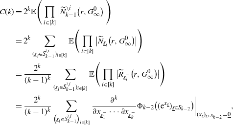 \begin{align*} C(k) & = 2^k\mathbb{E}\Bigg(\prod_{i \in [k]}\big|\widetilde{N}_{k-1}^{\setminus i}\big(r, G_{\infty}^0\big)\big|\Bigg) \\ & = 2^k\sum_{(\underline{s}_i \in S_{k-1}^{\setminus i})_{i \in [k]}} \mathbb{E}\Bigg(\prod_{i \in [k]}\big|\widetilde{N}_{\underline{s}_i}\big(r, G_{\infty}^0\big)\big|\Bigg) \\ & = \frac{2^k}{(k-1)^k}\sum_{(\underline{s}_i \in S_{k-1}^{\setminus i})_{i \in [k]}} \mathbb{E}\Bigg(\prod_{i \in [k]}\big|\widetilde{R}_{\underline{s}_i^-}\big(r, G_{\infty}^0\big)\big|\Bigg) \\ & = \frac{2^k}{(k-1)^k}\sum_{\big(\underline{s}_i \in S_{k-1}^{\setminus i}\big)_{i \in [k]}} \frac{\partial^k}{\partial x_{{\underline{s}_1^-}} \cdots \partial x_{{\underline{s}_k^-}}} \Phi_{k-2}\big((\textrm{e}^{x_{\underline{s}}})_{\underline{s} \in S_{k-2}}\big) \bigg|_{(x_{\underline{s}})_{\underline{s} \in S_{k-2}} = \underline{0}} , \end{align*}
which can be expressed explicitly using an iterated composition of the Lambert W function and elementary functions since the same is true for $\Phi_{k-2}$
by Lemma 4.4.
$\Phi_{k-2}$
by Lemma 4.4.
In particular, when $k=2$
, then
$k=2$
, then $\Phi_0(\textrm{e}^x) = \textrm{e}^x$
, and thus
$\Phi_0(\textrm{e}^x) = \textrm{e}^x$
, and thus $C(2)=4$
. When
$C(2)=4$
. When $k=3$
, by Lemma 4.4,
$k=3$
, by Lemma 4.4,
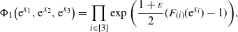 \begin{align*} \Phi_1\big(\textrm{e}^{x_1}, \textrm{e}^{x_2}, \textrm{e}^{x_3}\big) = \prod_{i \in [3]}\exp\bigg(\frac{1+\varepsilon}{2}(F_{(i)}(\textrm{e}^{x_i}) - 1)\bigg), \end{align*}
where, by (4.9), $F_{(i)}(z) = {-W\big({-}\frac{1}{2}\cdot\textrm{e}^{-{1}/{2}}\cdot z\big)}/{\frac{1}{2}}$
for any
$F_{(i)}(z) = {-W\big({-}\frac{1}{2}\cdot\textrm{e}^{-{1}/{2}}\cdot z\big)}/{\frac{1}{2}}$
for any $i \in [3]$
. Using the identities
$i \in [3]$
. Using the identities
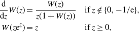 \begin{alignat*}{2} \frac{\textrm{d}}{\textrm{d}z} W(z) & = \frac{W(z)}{z(1 + W(z))} \quad & & \textrm{if } z \notin \{0, -1/\textrm{e}\}, \\ W(z\textrm{e}^z) & = z & & \textrm{if } z \ge 0, \end{alignat*}
we obtain $C(3)=32$
. Similarly, but with significantly more work, we obtain the value
$C(3)=32$
. Similarly, but with significantly more work, we obtain the value $C(4)=624$
. Recall that we obtained the same values for C(k) when
$C(4)=624$
. Recall that we obtained the same values for C(k) when $k \in \{ 2, 3, 4 \}$
using a different approach at the end of Section 4.1.
$k \in \{ 2, 3, 4 \}$
using a different approach at the end of Section 4.1.
5. The case of two colors
By Theorem 2.2, we know that the empirical color-avoiding connected component size densities converge. In this section, we give explicit formulas for their limit when there are only two colors.
First, we introduce some notation. Let $X \sim \textrm{Borel}(\mu)$
be a random variable. Given X, let us consider the random variable
$X \sim \textrm{Borel}(\mu)$
be a random variable. Given X, let us consider the random variable $Y \sim \textrm{Bin}(X-1, \theta)$
for some
$Y \sim \textrm{Bin}(X-1, \theta)$
for some $\theta \in [0,1]$
. Let
$\theta \in [0,1]$
. Let $q_{\mu, \theta} (\ell) \,:\!=\, \mathbb{P}(Y + 1 = \ell)$
,
$q_{\mu, \theta} (\ell) \,:\!=\, \mathbb{P}(Y + 1 = \ell)$
, $\ell=1,2,\dots$
It is not difficult to see that
$\ell=1,2,\dots$
It is not difficult to see that
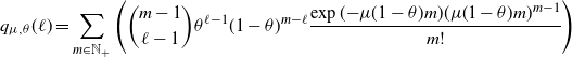 \begin{align*} q_{\mu, \theta}(\ell) = \sum_{m \in \mathbb{N}_+}\Bigg(\binom{m-1}{\ell - 1} \theta^{\ell - 1}(1 - \theta)^{m - \ell} \frac{\exp({-}\mu(1 - \theta)m)(\mu(1 - \theta)m)^{m-1}}{m!}\Bigg)\end{align*}
for any $\ell \in \mathbb{N}_+$
.
$\ell \in \mathbb{N}_+$
.
Proposition 5.1. Let $\lambda_{\textrm{red}}, \lambda_{\textrm{blue}} \in \mathbb{R}_+$
,
$\lambda_{\textrm{red}}, \lambda_{\textrm{blue}} \in \mathbb{R}_+$
, $\ell \in \mathbb{N}_+$
, and
$\ell \in \mathbb{N}_+$
, and $G_{\infty} \,:\!=\, G_{\infty}(r) \sim \mathcal{G}_{\infty}((\lambda_{\textrm{red}},\lambda_{\textrm{blue}}))$
be a two-colored ECBP tree. Let
$G_{\infty} \,:\!=\, G_{\infty}(r) \sim \mathcal{G}_{\infty}((\lambda_{\textrm{red}},\lambda_{\textrm{blue}}))$
be a two-colored ECBP tree. Let $\theta_{\textrm{blue}} \,:\!=\, \lambda^{\setminus \textrm{red}}$
and
$\theta_{\textrm{blue}} \,:\!=\, \lambda^{\setminus \textrm{red}}$
and $\theta_{\textrm{red}} \,:\!=\, \lambda^{\setminus \textrm{blue}}$
. Then
$\theta_{\textrm{red}} \,:\!=\, \lambda^{\setminus \textrm{blue}}$
. Then
 \begin{equation} f^*_{\ell} = \textbf{1}[\ell = 1]\widehat{p}^{\, *}((0, 0)) + q_{\lambda_{\textrm{red}}(1 - \theta_{\textrm{red}}),\,\theta_{\textrm{blue}}}(\ell)\widehat{p}^{\, *}((1, 0)) + q_{\lambda_{\textrm{blue}}(1 - \theta_{\textrm{blue}}),\,\theta_{\textrm{red}}}(\ell)\widehat{p}^{\, *}((1, 0)), \end{equation}
where
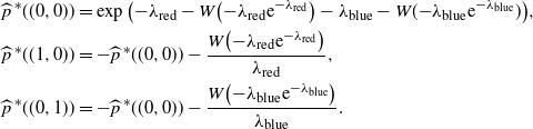 \begin{align*} \widehat{p}^{\, *}((0, 0)) & = \exp\big({-}\lambda_{\textrm{red}} - W\big({-}\lambda_{\textrm{red}}\textrm{e}^{-\lambda_{\textrm{red}}}\big) - \lambda_{\textrm{blue}} - W({-}\lambda_{\textrm{blue}}\textrm{e}^{-\lambda_{\textrm{blue}}})\big), \\ \widehat{p}^{\, *}((1, 0)) & = -\widehat{p}^{\, *}((0, 0)) - \frac{W\big({-}\lambda_{\textrm{red}}\textrm{e}^{-\lambda_{\textrm{red}}}\big)}{\lambda_{\textrm{red}}}, \\ \widehat{p}^{\, *}((0, 1)) & = -\widehat{p}^{\, *}((0, 0)) - \frac{W\big({-}\lambda_{\textrm{blue}}\textrm{e}^{-\lambda_{\textrm{blue}}}\big)}{\lambda_{\textrm{blue}}}. \end{align*}
Proof. By the definition of $f^*_{\ell}$
and by the total law of probability, we obtain
$f^*_{\ell}$
and by the total law of probability, we obtain
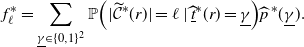 \begin{align*} f^*_{\ell} = \sum_{\underline{\gamma} \in \{0,1\}^2}\mathbb{P}\Big(|\widetilde{\mathcal{C}}^*(r)| = \ell \mid \underline{\widehat{t}}{}^*(r) = \underline{\gamma}\Big)\widehat{p}^{\, *}(\underline{\gamma}). \end{align*}
We examine the summands separately. Note that any red-avoiding path contains only blue edges, and similarly, any blue-avoiding path contains only red edges.
If $\underline{\gamma} = (1,1)$
then, by Lemma 3.2, we obtain
$\underline{\gamma} = (1,1)$
then, by Lemma 3.2, we obtain
 \begin{align*} \mathbb{P}\big(|\widetilde{\mathcal{C}}^*(r)| = \ell \mid \underline{\widehat{t}}{}^*(r) = (1,1)\big) \le \mathbb{P}\big(|\widetilde{\mathcal{C}}^*(r)| < \infty \mid \underline{t}^*(r) = (1,1)\big) = 0. \end{align*}
If $\underline{\gamma} = (0, 0)$
, then clearly
$\underline{\gamma} = (0, 0)$
, then clearly $\mathbb{P}\big(|\widetilde{\mathcal{C}}^*(r)| = \ell \mid \underline{\widehat{t}}{}^*(r) = (0, 0)\big) = \textbf{1}[\ell = 1]$
. If
$\mathbb{P}\big(|\widetilde{\mathcal{C}}^*(r)| = \ell \mid \underline{\widehat{t}}{}^*(r) = (0, 0)\big) = \textbf{1}[\ell = 1]$
. If $\underline{\gamma} = (1, 0)$
then, conditional on
$\underline{\gamma} = (1, 0)$
then, conditional on $\underline{\widehat{t}}{}^*(r) = (1, 0)$
, the branching process
$\underline{\widehat{t}}{}^*(r) = (1, 0)$
, the branching process $\big(\big|R_{\infty, d}^{\textrm{red}}\big|\big)_{d \in \mathbb{N}}$
is subcritical and has offspring distribution
$\big(\big|R_{\infty, d}^{\textrm{red}}\big|\big)_{d \in \mathbb{N}}$
is subcritical and has offspring distribution $\textrm{Poi}(\lambda_{\textrm{red}}(1-\theta_{\textrm{red}}))$
by [Reference Van der Hofstad31, Theorem 3.15]. Thus, the number of vertices of
$\textrm{Poi}(\lambda_{\textrm{red}}(1-\theta_{\textrm{red}}))$
by [Reference Van der Hofstad31, Theorem 3.15]. Thus, the number of vertices of $\big(\big|R_{\infty, d}^{\textrm{red}}\big|\big)_{d \in \mathbb{N}}$
has distribution
$\big(\big|R_{\infty, d}^{\textrm{red}}\big|\big)_{d \in \mathbb{N}}$
has distribution $\textrm{Borel}(\lambda_{\textrm{red}}(1-\theta_{\textrm{red}}))$
. In addition, each vertex of
$\textrm{Borel}(\lambda_{\textrm{red}}(1-\theta_{\textrm{red}}))$
. In addition, each vertex of $\big(R_{\infty, d}^{\textrm{red}}\big)_{d \in \mathbb{N}}$
is of type either (0, 0) or (1, 0) independently of each other with respective probabilities
$\big(R_{\infty, d}^{\textrm{red}}\big)_{d \in \mathbb{N}}$
is of type either (0, 0) or (1, 0) independently of each other with respective probabilities
 \begin{equation*} \frac{\widehat{p}^{\, *}((0, 0))}{\widehat{p}^{\, *}((0, 0)) + \widehat{p}^{\, *}((1, 0))} = \frac{(1 - \theta_{\textrm{blue}})(1 - \theta_{\textrm{red}})}{(1 - \theta_{\textrm{red}})} = 1 - \theta_{\textrm{blue}}, \qquad\!\!\! \frac{\widehat{p}^{\, *}((1, 0))}{\widehat{p}^{\, *}((0, 0)) + \widehat{p}^{\, *}((1, 0))} = \theta_{\textrm{blue}} . \end{equation*}
Thus, by the total law of probability,
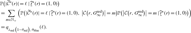 \begin{align*} & \mathbb{P}\big(|\widetilde{\mathcal{C}}^*(r)| = \ell \mid \underline{\widehat{t}}{}^*(r) = (1, 0)\big) \\ & = \sum_{m \in \mathbb{N}_+}\Big(\mathbb{P}\big(|\widetilde{\mathcal{C}}^*(r)| = \ell \mid \underline{\widehat{t}}{}^*(r) = (1, 0),\,\big|\mathcal{C}\big(r,G_{\infty}^{\textrm{red}}\big)\big| = m\big) \mathbb{P}\big(\big|\mathcal{C}\big(r,G_{\infty}^{\textrm{red}}\big)\big| = m \mid \underline{\widehat{t}}{}^*(r) = (1, 0)\big)\Big) \\ & = q_{\lambda_{\textrm{red}} \big(1 - \theta_{\textrm{red}}\big), \, \theta_{\textrm{blue}}} (\ell). \end{align*}
If $\underline{\gamma} = (0, 1)$
then, similarly,
$\underline{\gamma} = (0, 1)$
then, similarly, $\mathbb{P}\big(|\widetilde{\mathcal{C}}^*(r)| = \ell \mid \underline{\widehat{t}}{}^*(r) = (0, 1)\big) = q_{\lambda_{\textrm{blue}}(1 - \theta_{\textrm{blue}}), \, \theta_{\textrm{red}}}$
. Therefore, (5.1) holds. By (4.4), we obtain
$\mathbb{P}\big(|\widetilde{\mathcal{C}}^*(r)| = \ell \mid \underline{\widehat{t}}{}^*(r) = (0, 1)\big) = q_{\lambda_{\textrm{blue}}(1 - \theta_{\textrm{blue}}), \, \theta_{\textrm{red}}}$
. Therefore, (5.1) holds. By (4.4), we obtain
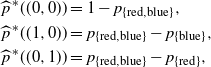 \begin{align*} \widehat{p}^{\, *}((0, 0)) & = 1 - p_{\{\textrm{red}, \textrm{blue}\}}, \\ \widehat{p}^{\, *}((1, 0)) & = p_{\{\textrm{red}, \textrm{blue}\}} - p_{\{\textrm{blue}\}}, \\ \widehat{p}^{\, *}((0, 1)) & = p_{\{\textrm{red}, \textrm{blue}\}} - p_{\{\textrm{red}\}}, \end{align*}
and, by Corollary 4.1, the stated result follows.
6. Open questions
We conclude our paper with a list of open questions and conjectures that we propose for future research.
In Section 4 we gave explicit, recursive formulas for the asymptotic density $f^*_{\infty}$
of the giant color-avoiding connected component, and in Section 5 we gave a formula for the asymptotic density
$f^*_{\infty}$
of the giant color-avoiding connected component, and in Section 5 we gave a formula for the asymptotic density $f^*_{\ell}$
of the set of vertices that belong to a color-avoiding connected component of size
$f^*_{\ell}$
of the set of vertices that belong to a color-avoiding connected component of size $\ell$
for any
$\ell$
for any $\ell \in \mathbb{N}_+$
in the case of
$\ell \in \mathbb{N}_+$
in the case of $k=2$
colors.
$k=2$
colors.
Question 6.1.
Is there an explicit formula for $f^*_{\ell}$
for any
$f^*_{\ell}$
for any $\ell \in \mathbb{N}_+$
and for
$\ell \in \mathbb{N}_+$
and for $k \ge 3$
colors?
$k \ge 3$
colors?
It is well known (see [Reference Aldous2] and the references therein) that the cardinality of the union of the largest components in an (uncolored) critical Erdős–Rényi graph $G_n$
with n vertices is of order
$G_n$
with n vertices is of order $n^{2/3}$
. It follows from Theorem 2.2 and Proposition 2.1 that if
$n^{2/3}$
. It follows from Theorem 2.2 and Proposition 2.1 that if $\lambda^{\setminus i} = 1$
for some
$\lambda^{\setminus i} = 1$
for some $i \in [k]$
, then
$i \in [k]$
, then $({1}/{n})\max_{v \in V(G_n)}|\widetilde{\mathcal{C}}(v,G_n)| \stackrel{\mathbb{P}}{\longrightarrow} 0$
as
$({1}/{n})\max_{v \in V(G_n)}|\widetilde{\mathcal{C}}(v,G_n)| \stackrel{\mathbb{P}}{\longrightarrow} 0$
as $n \to \infty$
.
$n \to \infty$
.
Question 6.2.
Let $k \in \mathbb{N}_+$
,
$k \in \mathbb{N}_+$
, $\underline{\lambda} \in \mathbb{R}_+^k$
, and let
$\underline{\lambda} \in \mathbb{R}_+^k$
, and let $G_n \sim \mathcal{G}_n([n],\underline{\lambda})$
for all
$G_n \sim \mathcal{G}_n([n],\underline{\lambda})$
for all $n \in \mathbb{N}_+$
. What is the order of magnitude of
$n \in \mathbb{N}_+$
. What is the order of magnitude of $\max_{v \in [n]}|\widetilde{\mathcal{C}}(v, G_n)|$
if
$\max_{v \in [n]}|\widetilde{\mathcal{C}}(v, G_n)|$
if $\lambda^{\setminus i} = 1$
for some
$\lambda^{\setminus i} = 1$
for some $i \in [k]$
, and in particular, if
$i \in [k]$
, and in particular, if $\lambda^{\setminus i} = 1$
for all
$\lambda^{\setminus i} = 1$
for all $i \in [k]$
?
$i \in [k]$
?
Note that [Reference Lichev and Schapira20] contains some results in the vein of our Question 6.2; see their Theorem 1.1 and Proposition 1.3.
We know from Theorem 2.1 that C(k) is an integer if $k \in \{ 2, 3, 4 \}$
.
$k \in \{ 2, 3, 4 \}$
.
Question 6.3. Is C(k) an integer for all $k \in \mathbb{N}_+$
?
$k \in \mathbb{N}_+$
?
Our results pertain to one of the most fundamental edge-colored random graph models, i.e. the edge-colored Erdős–Rényi graph. A natural, more heterogeneous, model of edge-colored random graphs is the following generalization of the well-known configuration model [Reference Van der Hofstad32, Section 1.3]. Let $k \in \mathbb{N}_+$
and let
$k \in \mathbb{N}_+$
and let $p\colon \mathbb{N}_+^k \to [0,1]$
satisfying
$p\colon \mathbb{N}_+^k \to [0,1]$
satisfying $\sum_{\underline{d} \in \mathbb{N}_+^k} p(\underline{d}) = 1$
. We consider a sequence of edge-colored graphs
$\sum_{\underline{d} \in \mathbb{N}_+^k} p(\underline{d}) = 1$
. We consider a sequence of edge-colored graphs $G_n$
where the edge-colored degree sequence satisfies
$G_n$
where the edge-colored degree sequence satisfies
and the half-edges of the same color are matched according to the rules of the configuration model.
Question 6.4. Does Theorem 2.2 have an analogue in the above-described edge-colored configuration model? Is there an explicit formula for the asymptotic density of the largest color-avoiding connected component?
Color-avoiding percolation was first introduced for vertex-colored graphs [Reference Krause, Danziger and Zlatić15, Reference Krause, Danziger and Zlatić16]. The definition of color-avoiding connectivity in vertex-colored graphs is ambiguous. The two most interesting versions are as follows. In the first version, two vertices are color-avoiding connected in a vertex-colored graph if there exists a path between them whose internal vertices are not of color i for any color i. Whereas in the second version, two vertices are color-avoiding connected if there exists a path between them using any colors and either at least one of the vertices is of color i or there exists a path between them whose vertices are not of color i for any color i. In [Reference Molontay and Varga24], we showed that these two definitions can yield problems with highly different computational complexity.
Question 6.5. Does Theorem 2.2 have an analogue in a vertex-colored Erdős–Rényi random graph, i.e. in an Erdős–Rényi random graph whose vertices are randomly colored? Is there an explicit formula for the asymptotic density of the largest color-avoiding connected component?
Funding information
The research of Roland Molontay, Balázs Ráth, and Kitti Varga was partially supported by grant NKFI-FK-123962 of NKFI (National Research, Development and Innovation Office). The research of Panna Tímea Fekete and Balázs Ráth was partially supported by the ERC Synergy under Grant No. 810115 – DYNASNET. Panna Tímea Fekete’s Project No. 1016492. has been implemented with the support provided by the Ministry of Culture and Innovation of Hungary from the National Research, Development and Innovation Fund, financed under the KDP-2020 funding scheme, and her research was partially supported by the National Research, Development and Innovation Office under Grant No. 2018-2.1.1.-UK_GYAK-2018-00008. The research of Roland Molontay was partially supported by NKFIH 142169 research grant.
Competing interests
There were no competing interests to declare which arose during the preparation or publication process of this article.


