


1. Introduction
In economies where large populations live on <$1 per day, how much can households smooth consumption over the lifecycle? While a lot of attention has been drawn to the testing of the informal arrangements that preserve consumption in response to income shocks (i.e., unanticipated income changes) in poor countries [Townsend (Reference Townsend1994); Attanasio and Ríos-Rull (Reference Attanasio and Ríos-Rull2000); Kinnan (Reference Kinnan2014)], less is known about the ability to smooth consumption against anticipated changes in income such as the arrival of old age. This is particularly important for poor countries where the lack of a pension system goes hand in hand with the presence of savings constraints [Dupas and Robinson (Reference Dupas and Robinson2013a, Reference Dupas and Robinson2013b); Brune et al. (Reference Brune, Giné, Goldberg and Yang2015)] and with a low ability to accumulate wealth over the lifecycle [De Magalhães and Santaeulàlia-Llopis (Reference De Magalhães and Santaeulàlia-Llopis2018)]. This can limit the ability to sustain consumption in old age. To assess this question, we draw on the new waves of the Integrated Surveys on Agriculture (ISA) under the Living Standards Measurement Study (LSMS) in Sub-Saharan Africa (SSA).Footnote 1 We focus on some of the world poorest countries in SSA, mainly Malawi, where lifecycle consumption smoothing can be a strong challenge.Footnote 2 Three main empirical findings emerge from our analysis.
Our first finding is that the household's ability to smooth consumption over the lifecycle is large in SSA, particularly in rural areas. For the purpose of this paper, we define consumption smoothing over the lifecycle as holding marginal utilities relatively constant across stages of life [Browning and Crossley (Reference Browning and Crossley2001)]. Household expenditure displays a hump shape over the lifecycle in both urban and rural areas, but the hump is much less pronounced in rural areas. This implies a larger ability to smooth lifecycle consumption in rural areas than in urban areas. The difference between urban and rural expenditure profiles also holds once we control for household structure. Precisely, the size of the adult-equivalent expenditure hump for urban areas is roughly double that for rural areas. Further, disaggregating lifecycle expenditure we find that food expenditure is twice smoother over the lifecycle than nonfood expenditure which, given the larger share of food in household expenditure in rural areas, partly explains the flatter profile of household expenditure in rural areas than in urban areas.
The presence of a hump in lifecycle expenditure in SSA is consistent with previous evidence from rich and middle-income countries [Deaton and Paxson (Reference Deaton and Paxson1994); Attanasio et al. (Reference Attanasio, Banks, Meghir and Weber1999); Storesletten et al. (Reference Storesletten, Telmer and Yaron2004); Fernández-Villaverde and Krueger (Reference Fernández-Villaverde and Krueger2007)]. Interestingly, the size of the hump in household expenditure in the urban areas of SSA is comparable to the United States. This implies that lifecycle consumption is smoother in the rural areas of SSA, where the vast majority of the population lives than in the United States.Footnote 3
Our second finding is that the smoothing of food expenditure is driven by substituting into self-farmed staple food (e.g., maize in Malawi) and away from purchased food in old age.Footnote 4 Food gifts play a minor role in lifecycle smoothing as they are flat throughout. These findings lessen the role of traditional lifecycle savings and sharing networks as explanations of how consumption smoothing is achieved in old age in the poor countries that we study. First, the decline in purchased food in old age together with a low ability to accumulate wealth and dissave implies that a large amount of lifecycle consumption smoothing that we document cannot be solely achieved through traditional savings as the standard lifecycle model predicts.Footnote 5 Second, despite the important role of informal arrangements in managing consumption insurance against unanticipated changes in income in poor countries [Townsend (Reference Townsend1994); Kinnan (Reference Kinnan2014)], food gifts remain relatively constant across stages of life and hence do not contribute to consumption over the lifecycle.Footnote 6
An important aspect of lifecycle smoothing is potential differences between food expenditure and consumption (measured in caloric intake) [Aguiar and Hurst (Reference Aguiar and Hurst2005)]. This is particularly relevant in poor countries where food is the largest item of the consumption basket. In addition, price levels might differ across space even within rural and urban areas [Deaton and Dupriez (Reference Deaton and Dupriez2011); Gaddis (Reference Gaddis2015)].Footnote 7 To abstract from prices and investigate differences between expenditure and consumption we study the lifecycle behavior of total caloric intake. We find that the lifecycle profile of caloric intake is considerably smoother than the lifecycle profile of food expenditure. Household caloric intake practically shows no hump over the lifecycle in SSA despite there being a hump in food expenditure. This result is closely related to the findings in Aguiar and Hurst (Reference Aguiar and Hurst2005) for the United States and Hicks (Reference Hicks2015) for Mexico. These authors show that food consumption remains stable with age as retired households substitute away from eating out and spend more time shopping and preparing food at home. In contrast to these authors, the smoothing strategy in SSA consists of substituting away from purchased food and into self-farmed food.
Our third finding is that this smoothing strategy has two costly consequences. The first cost is that school-age children in households headed by the elderly work more hours and are less likely to attend school. Children in a household with an elderly head are 31% less likely to attend school when compared to children in households with young heads. While the household head and spouse decrease the number of hours worked in old age, the hours spent in self-farming by their cohabiting adult children increases by 15% and that of school-age children by 20% over the lifecycle. This link between the age of the household and labor supply speaks to the result of LaFave and Thomas (Reference LaFave and Thomas2016). They provide empirical results rejecting the validity of the farm household model that assumes complete markets. Were markets complete, the household decision on how much labor to use should be independent of the household composition (age of the head and household size). They show that this is not the case with Indonesian data. We find that this is not the case in Malawi either. Our results suggest that in an economy where traditional savings mechanisms are not available, households use their own children (during their school years and as adults) to increase labor supply into self-farming as the household head ages—even though these members may be better employed elsewhere (e.g., school-age children should be attending school).
The second cost is a decrease in the nutritional quality of the household food intake as the head reaches old age. Maize consumption in Malawi, for example, rises over the lifecycle and provides calories and iron, but not much more. There is a household-level decrease in the intake of micronutrients such as vitamin A, B12, C, and D, and macronutrients such as sugar and fat.Footnote 8 On the top of working more hours with less schooling, a less nutritious diet can diminish the ability of school-age children to acquire human capital [Schultz (Reference Schultz1999); Behrman (Reference Behrman2009); Maluccio et al. (Reference Maluccio, Hoddinott, Behrman, Martorell, Quisumbing and Stein2009)] and cognitive skills [Feyrer et al. (Reference Feyrer, Politi and Weil2013)].Footnote 9 Thus, the young children bear a double burden from the main consumption smoothing strategy in SSA. Further, the struggle to smooth caloric intake in old age by turning into self-farming directly speaks to the literature on the “Food Problem” [Schultz (Reference Schultz1953); Timmer (Reference Timmer2002)] which can have long-term implications for aggregate development [Gollin et al. (Reference Gollin, Parente and Rogerson2007)]. In particular, in order to meet subsistence needs, adult children cohabiting with elderly heads focus on self-farming instead of looking for alternative occupations in more productive sectors [Gollin et al. (Reference Gollin, Lagakos and Waugh2014)].
Our paper relates closely to Oliveira (Reference Oliveira2016), who uses the incidence of identical twins to infer the causal effect of family size on old age support in China. An elderly household with larger families are more likely to have a co-habiting child and receive more transfers. In Malawi, we find that 56% of elderly households (head aged 55 or more) have at least one cohabiting adult child and 66% has at least one school-age child. This is consistent with results for China where 32% of elderly households cohabit with an adult child. We go beyond Oliveira (Reference Oliveira2016)'s results in showing the cost of old-age support strategy: less schooling for school-age children and lower nutritional quality of household food intake. Our findings also give empirical support to the trade-off between fertility and savings as a way to cope with old age [Boldrin and Jones (Reference Boldrin and Jones2002); Banerjee et al. (Reference Banerjee, Meng, Porzio and Qian2014)].Footnote 10 Our contribution is to discuss a precise mechanism through which children help the elderly cope with consumption in old age in SSA economies such as Malawi: cohabitation and an increase in hours devoted to self-farming as opposed to alternative mechanisms such as lifecycle savings and food gifts.Footnote 11
The rest of the paper proceeds as follows. Section 2 describes our data and discusses the construction of household consumption and expenditure. In Section 3, we specify our empirical strategy based on a simple lifecycle model with two consumption goods. Our main empirical results are discussed in Section 4. We conclude in Section 5.
2. Data and measurement issues
We work with the ISA recently collected under the umbrella of the LSMS of the World Bank. The ISAs are seen as a clear improvement on previous LSMS rounds [Carletto et al. (Reference Carletto, Beegle, Himelein, Kilic, Murray, Oseni, Scott and Steele2010)] and they are unique in the level of detail on nondurable and durable consumption [Beegle et al. (Reference Beegle, De Weerdt, Friedman and Gibson2012)].Footnote 12 We focus the discussion on Malawi because it has the most detailed ISA questionnaire and the largest sample size with two cross-sectional waves; 11,280 in 2004/05 and 12,271 in 2010/11, and an additional panel wave between 2010 and 2013 of 3,247 households.Footnote 13 Parallel results for Uganda and Nigeria are available in the online Appendix. The surveys in Uganda and Nigeria have a smaller sample, respectively 3,200 and 5,000 households per wave. There are three waves for Uganda (2005/06, 2009/10, 2010/11, 2011/2012) and two for Nigeria (2010/11 and 2012/13). Using 2010 as a comparison year, 84% of the Malawi sample is rural; respectively, 71% and 85% in Nigeria and Uganda.
The ISAs are particularly detailed in capturing food consumption. Food consumed is recorded by origin including purchases, self-farmed production and received gifts. To construct food expenditure we attach consumption prices to the quantities of self-farmed food and food gifts.Footnote 14 This way, our measure of food expenditure includes not only food purchases but also self-farmed food and food gifts. This is essential for the SSA countries that we study because the value of self-farmed food represents close to 50% of the total value of household food expenditure, and the total value of food expenditure is roughly 60% of total expenditure [De Magalhães and Santaeulàlia-Llopis (Reference Deaton2018)].
Seasonality is an important aspect of consumption in SSA that deserve further discussion. This is particularly relevant for food consumption, which is reported with a 7-day recall (other consumption items are usually reported with longer recalls). Given the short recall period, food consumption may exhibit monthly patterns [Paxson (Reference Paxson1993)]. Since the Malawi surveys in 2004/05 and 2010/11 are rolled out across the year from March to March, we can control for seasonality with monthly dummies.Footnote 15 Once the value of food consumption has been deseasonalized, we create a measure of total food expenditure: the sum of food purchases and the monetary value of self-farmed food and received food gifts.Footnote 16
Direct measures of food consumption, i.e., the intake of calories and other micro and/or macronutrients, help circumvent problems of measurement relating to prices. In this direction, the ISAs allow us to isolate the effects of prices and distinguish between consumption and expenditure because the quantity of food consumed is also carefully recorded. These quantities are reported in units that must be converted to kilograms.Footnote 17 The survey for Malawi allows for 135 separate food items to be reported and includes any items consumed outside the home. With such level of detail, the food basket of Malawian household can be accurately recovered.Footnote 18 We use the Food Composition Tables from the United States Department of Agriculture (USDA) National Nutrient Database to compute the nutritional intake of each and all of the food items consumed. In our analysis, we include calories and other macro-nutrients (fat and sugar), minerals (iron and zinc), and vitamins (A, B12, C, and D); see our discussion in Section 4.2.Footnote 19
Nondurable expenditure other than food (62% of average household consumption in Malawi) are classified under alcohol and tobacco (negligible), clothing (3%), health (i.e., prevention, treatment, hospitalization, and traditional healers—2%), education (2%), utilities (15%), housing (i.e, mostly self-reported rental value of dwelling or rent—2%), transportation (1%), and other nondurables (13%).Footnote 20 This level of detail is similar in the Nigeria and Uganda surveys.
3. Theory and empirical strategy
We present a lifecycle model à la Attanasio et al. (Reference Attanasio, Banks, Meghir and Weber1999) to guide our empirical analysis in Section 3.1. Importantly, we distinguish between food and nonfood consumption. We discuss household structure in Section 3.2 and our empirical strategy in Section 3.3.
3.1. A lifecycle model with two consumption goods: food and nonfood
A household lives for a finite number of periods until age J. Each household maximizes lifetime utility by choosing age profiles of household food consumption, c a,j, and household nonfood consumption, c m,j, as follows:
 $$\mathop {\max} \limits_{\{ c_{a,j},c_{m,j},a_j\} _{\,j = 0}^J} \mathop \sum \limits_{\,j = 0}^J \beta ^j[ {u\lpar {c_{a,j}} \rpar \exp {\rm \;} (\theta_a^{\rm{\prime}} z_j) + \kappa v\lpar {c_{m,j}} \rpar \exp {\rm \;} (\theta_m^{\rm{\prime}} z_j)} ],$$
subject to a budget constraint p ac a,j + c m,j + a j+1 = y j + (1 + r)a j given a 0 and an income stream  $\{ y_j\} _0^J $. We denote with p a the relative price of food in terms of nonfood consumption good and a j is a risk-free asset with a constant return r. We assume additive separability of the utility function across consumption goods as is standard in the structural transformation literature [Gollin et al. (Reference Gollin, Parente and Rogerson2002, Reference Gollin, Parente and Rogerson2007)]. In our preferences we have a time discount factor β and a set of household characteristics that may affect each consumption good differently; κ denotes the weight of non-food consumption relative to food consumption. We denote the household characteristics as vector z j, namely household structure. Since household structure may have different effects across consumption goods, through the vectors θ a and θ m, each household member may potentially have a different share per consumption good [Aguiar and Hurst (Reference Aguiar and Hurst2014)]. For example, children might require a higher share of food consumption than of other consumption goods.
Our model implies that households smooth both food and nonfood consumption in the sense of holding marginal utility constant over the lifecycle. This simply means that consumption follows the Euler equations (one per consumption good).Footnote 21 Moreover, assuming a constant relative risk aversion (CRRA) utility function separately for food and for nonfood consumption with coefficients η a ≥ 0 and η m ≥ 0, respectively, we can rewrite the Euler equations after taking logs as
 $$\ln \,{\rm \;} c_{i,j + 1}-\ln {\rm \;} \,c_{i,j} = {\rm cons}. + \displaystyle{1 \over {\eta _i}}\;\theta _i^{\rm {\prime}} \lpar {z_{\,j + 1}-z_j} \rpar $$
for i = {a, m} and the constant is (1/η i)ln β(1 + r). If β(1 + r) is larger (smaller) than one consumption linearly increases (decreases) over the life cycle. Then, note that only changes in household structure z j can generate nonlinear paths (i.e, humps) in consumption over the lifecycle. We empirically test equation (3) separately for rural and urban areas. Before that, we explore the behavior of household structure over the lifecycle.
3.2. Household structure over the lifecycle
We document the behavior of household structure by household heads' age groups separately for rural and urban areas for Malawi.Footnote 22 The age of the head is a good indicator for the age of the household. Only 3.7% of households have an adult that is at least 5 years older than the head.Footnote 23 The average age of household heads is larger in rural areas, 43 than in urban areas, 39. Overall, household size shows a clear lifecycle hump in both rural and urban areas (Table 1).
Table 1. Household Structure (Malawi ISA 2010/11)
Notes: The data refer to the Malawi ISA 2010/11. We obtain similar insights for the alternative Malawi ISA surveys in 2004/05 and 2013. Children are defined as sons, daughters, nephews, nieces, grandchildren, or adopted/fostered children of the household head. Adult children refer to the household's head sons and daughters aged 19 or above. The relationship between each member of the household and the household head is collected in the household roster that includes relatives and non-relatives (e.g. servants and lodgers) living in the household at least 9 months in the last year.
Household heads in both rural and urban areas are predominantly married with 70% of heads having a cohabiting spouse in rural areas and 71% in urban areas.Footnote 24 In rural areas, 70% of heads aged 15–24 have a cohabiting spouse, a figure that increases to roughly 80% for heads aged 25–44 and slowly decreases thereafter to reach 50% for heads aged more than 65 (panel A2, Table 1). Urban areas follow a similar pattern (panel B2, Table 1).Footnote 25
The number of school-age children in rural households peaks among heads aged 35–44. These households have an average of 3.7 school-age children (rows 2 and 3, Panel A2, Table 1). This number decreases gradually to 1.5 for heads aged above 65. A less prominent hump is present in urban areas. A child is defined as a son, daughter, nephew, niece, grandchild, or an adopted/fostered child of the household head.Footnote 26
The number of adult children cohabiting with the head mostly increases over the lifecycle.Footnote 27 In rural areas, the number of cohabiting adults peaks at 0.8 for heads aged 55–64, and then drops to 0.5 for heads above 65. In urban areas, the peak occurs at 1.5 for heads aged 55–64 and remains high at 1.2 for heads above 65. As we will see below, a substitution away from purchased food towards home-produced foods is a key mechanism to smooth consumption in old age. The number of adult and school-age children living with elderly parents (and helping with home production) may be an important channel through which households maintain their level of household consumption when the head reaches old age.
3.3 Empirical strategy
We now empirically assess the ability of rural and urban households to smooth lifecycle consumption defined as keeping marginal utilities relatively constant across stages of life as per equation (3). It is common practice to directly assess smoothing behavior over the lifecycle by studying the age profiles of expenditure in panels of cross-sectional data [Aguiar and Hurst (Reference Aguiar and Hurst2014)].
3.3.1 Household-level specification
We estimate the mean lifecycle profiles of household-level expenditure with the following regression:
 $$\ln {\rm \;} \,C_{it}^k = \beta _0^k + f\lpar {a_{it};{\rm \Theta}} \rpar + 1_t\beta _t^k t + 1_b\beta _b^k b + \epsilon _{it}^k, $$
where  $C_{it}^k $ is the household expenditure of household i during period t on expenditure category k (e.g., food and nonfood); a it is the age of the household head (for ages 26–65) and f(a; Θ) is a function relating age and expenditure; t are time dummies for each household survey (e.g., Malawi ISA 2004/05, 2010/11, and 2013); b are cohort dummies;Footnote 28 and $\beta _0^k $ is the expenditure level of category k at age 25.
Our first and benchmark specification does not impose any restriction on the functional form between age and consumption, and we represent f(a it, Θ) with a full set of age dummies, i.e.,  $1_a\beta _a^k a_{it}$. Note that under this specification age, time, and cohort effects are not linearly independent from each other (i.e., b = t − a) and only two of the three dummy controls can be operative [Deaton (Reference Deaton1997); Heathcote et al. (Reference Heathcote, Storesletten and Violante2005)]. That is, the identification of β a requires additional assumptions. Our benchmark specification is defined by age and time controls only, i.e., we drop the cohort effects from equation (4). This choice is guided by the historical events in these economies that suggest that time effects unambiguously play a key role. For example, Malawi faced a famine the year before the 2004/05 survey and by 2010/11 the economy had not only recovered fully but a program of widespread fertilizer subsidy had been implemented. To assess whether cohorts effects shape our estimated age profiles we also consider a second specification in which we assume a cubic polynomial form for f(a it, Θ). This avoids the multicollinearity issue discussed above and allows us to keep both time dummies and cohort dummies.Footnote 29 Our results are robust to this alternative specification. In the main text, we present results from the our benchmark (and arguably more parsimonious) specification. We refer the reader to the online Appendix for the estimates of our alternative specification.
3.3.2 Adult-equivalent specification
Given equation (3) (i.e., the Euler equation) we now additionally control for household structure and estimate lifecycle profiles of adult-equivalent expenditure as follows:
 $$\ln \,C_{it}^k = \beta _0^k + f\lpar {a_{it};{\rm \Theta}} \rpar + 1_t\beta _t^k t + 1_b\beta _b^k b + \theta _{it}^k X_{it} + \epsilon _{it}^k, $$
where X it is an additional vector of household structure characteristics that includes dummy variables for marital status, household size, and the number of male and female children in age categories 1–2, 3–5, 6–13, and 14–18. This implies that we take the equivalence scales (and household structure) as exogenous, as in Aguiar and Hurst (Reference Aguiar and Hurst2014). The only difference is that we allow for the gender of the child and a thinner set of age categories of children defined as individuals under 18.Footnote 30 Again, as it was the case with the household-level specification, with the adult-equivalent specification we also focus in the main text on the results from our benchmark specification with age and time controls only, i.e., without cohort dummies. In the online Appendix, we show the results for the alternative specification that imposes a cubic polynomial on f(a it;Θ) and controls for both time and cohort dummies.Footnote 31
4. Empirical results
First, we focus on lifecycle expenditure. We emphasize the differential behavior of rural and urban areas, food and nonfood expenditure, and the role of self-farming (Section 4.1). Second, we investigate the lifecycle behavior of consumption in terms of caloric intake and maize consumption (in kilograms) (Section 4.2). Third, we examine the consequences of lifecycle smoothing for child investments and nutrient intake (Section 4.3). Unless otherwise noted, our results focus on Malawi with more details on other SSA countries in the online Appendix.
4.1. Lifecycle expenditure
We show the age profile of household-level nondurable expenditure (in logs) in Figure 1 using our more parsimonious specification described in Section 3.3 that control for time only. To facilitate exposition, the age profiles estimated with equations (4) and (5) are plotted after they have been normalized so that the value of the age dummy at age 25 is 0 (in logs). We plot these normalized age effects as well as a cubic polynomial that approximates the age effects.Footnote 32 Before dissecting the lifecycle behavior of household expenditure in poor countries, we contextualize it with respect to the United States [panel (a), Figure 1]. Nationwide, household expenditure in Malawi increase by 0.25 log points between the age of 25 and its peak in the early 40s, while household expenditure in the United States increases by roughly twice as much, 0.42 log points, between the ages of 25 and its peak, somewhat later than Malawi, in the late 40s. That is, there is a clear lifecycle hump in nondurable expenditure in both countries but it is twice as prominent in the United States as in Malawi.
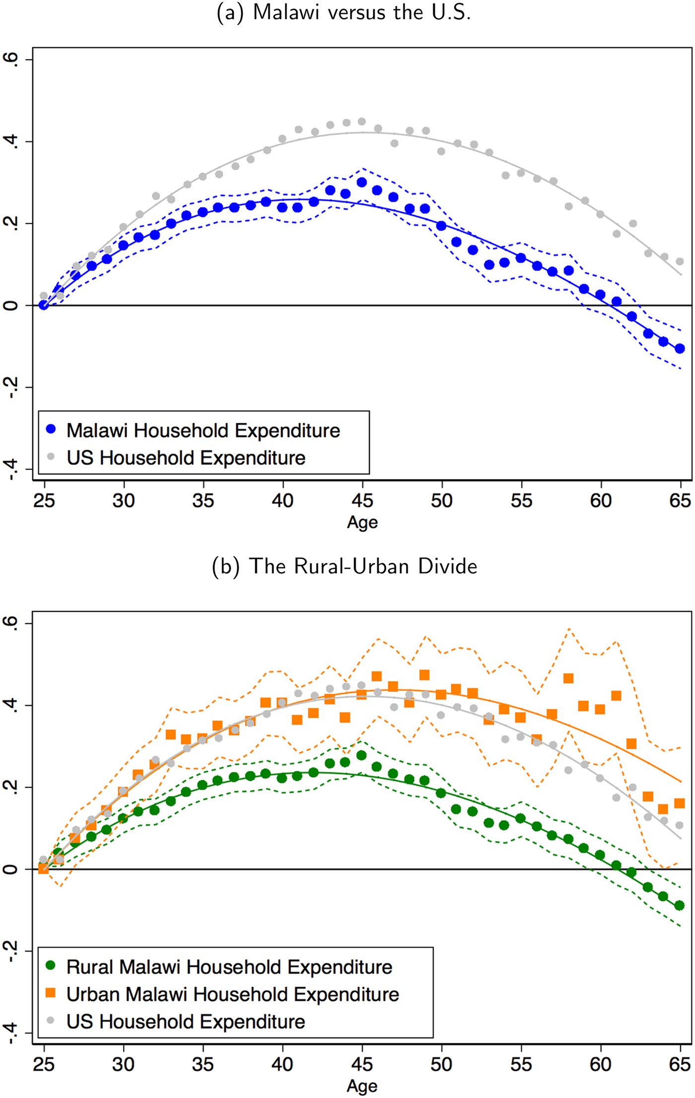
Figure 1. Lifecycle household expenditure: Malawi, the United States and the rural-urban divide.
4.1.1 The rural-urban divide
A potential explanation behind the nationwide differentials across countries is the rural-urban composition of the population. In Malawi, roughly 85% of the population lives in rural areas, while this figure is <1% in the United States. We explore the lifecycle behavior of household expenditure separately for rural and urban Malawi [panel (b), Figure 1]. In rural areas, the peak in nondurable expenditure is reached at 0.23 log points in the early 40s. The nondurable expenditure in urban areas peaks at 0.46 log points in the late 40s. Beyond the peak, nondurable expenditure reaches back the initial level at age 60 in rural areas with log deviation of −0.11 at age 65, while it remains always above the initial level in urban areas with a log deviation of 0.20 at age 65. This implies that the total range of household expenditure from its peak to its minimum is 0.34 log points in rural areas and 0.46 log points in urban areas, suggesting more lifecycle consumption smoothing in rural areas than in urban areas. The rural-urban divide largely accounts for the nationwide behavior of nondurable expenditure over the lifecycle: nationwide expenditure follows the behavior of rural areas. Interestingly, lifecycle expenditure in urban Malawi closely follows its U.S. counterpart [panel (b), Figure 1].
To examine the lifecycle effect of household structure, we compare the estimated age profiles from our household-level specification [equation (4)] against the same estimates from our adult-equivalent specification that controls for household structure characteristics [equation (5)]. We show the age profiles when we control for household structure separately for rural and urban areas in Figure 2. Adult-equivalent expenditure shows a hump that peaks lower and at an earlier age over the lifecycle than its household-level counterpart. In rural areas, adult-equivalent expenditure increases by 0.06 log points from age 25 to its peak age. That is, household structure accounts for more than 2/3 of the lifecycle hump in expenditure in rural areas. In urban areas, adult-equivalent expenditure increases by 0.30 log points from age 25 to its peak age. This implies that household structure accounts for roughly 1/3 of the lifecycle hump in expenditure in urban areas.Footnote 33 Note that adult-equivalent expenditure has a higher peak and a steeper decline during old age in urban areas than in rural areas. The total range of adult-equivalent nondurable expenditure from its peak to its minimum at age 65 is 0.23 log points in rural areas and 0.39 log points in urban areas. This implies that, after controlling for household structure, we find twice more consumption smoothing in rural areas than in urban areas.
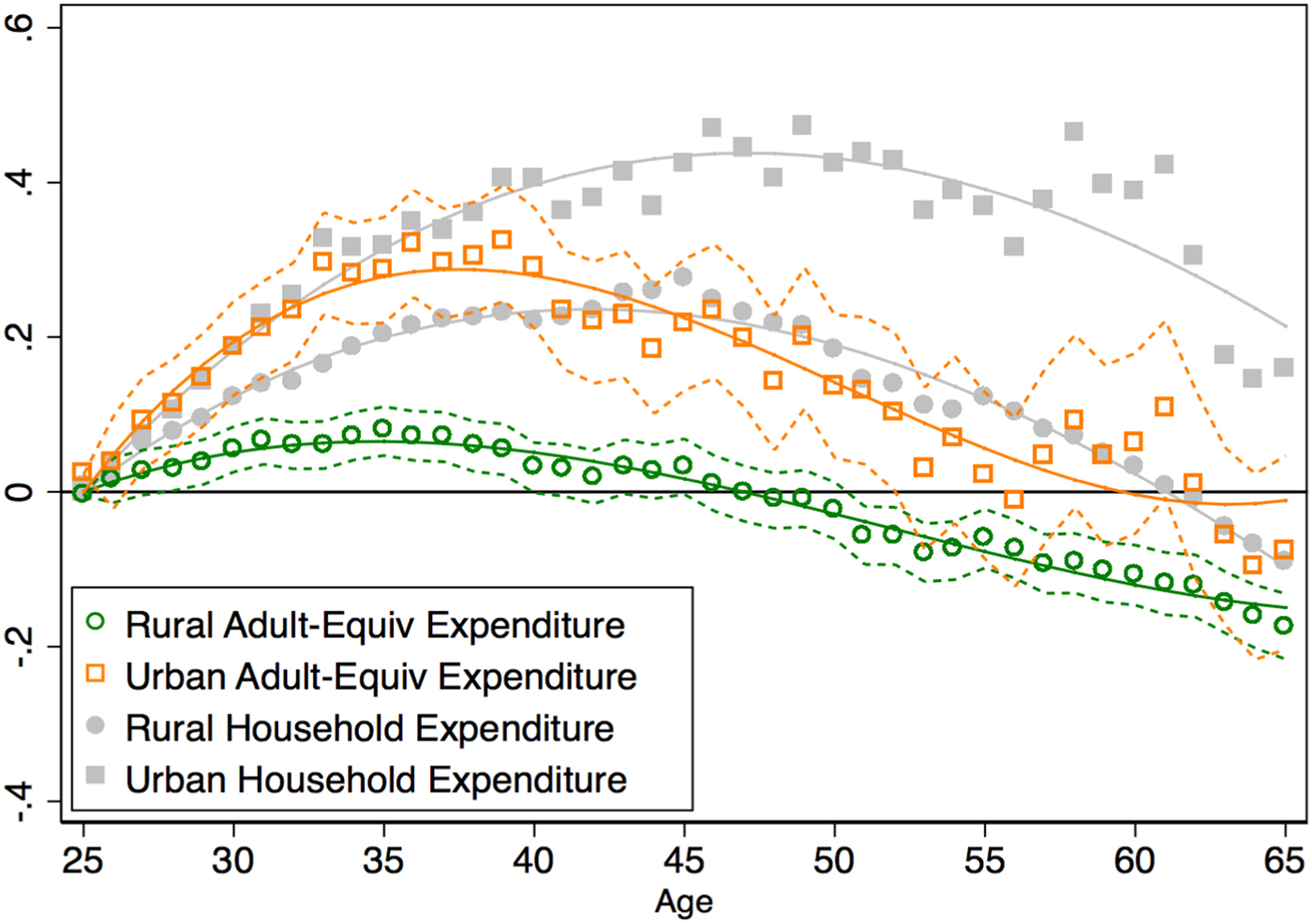
Figure 2. The role of household structure.
4.1.2 Food and nonfood expenditure
To examine the source of the hump in adult-equivalent nondurable expenditure, we decompose the lifecycle profiles into food and nonfood. Food expenditure [panel (a), Figure 3] is smoother than nonfood expenditure [panel (b), Figure 3]. In rural areas, food expenditure and nonfood expenditure peak in the early 30s at a similar level to age 25, a deviation of 0.06 log points, but the decline after the peak is starker for nonfood expenditure. Nonfood expenditure declines to −0.31 log points at age 65, while food expenditure declines by −0.13 log points. In urban areas, nonfood expenditure peaks at a larger level than food expenditure, respectively, by a deviation of 0.33 and 0.23 log points in the late 30s. As it was the case in rural areas, the decline in old age for nonfood expenditure is roughly three times larger than for food expenditure in urban areas. The total range of food expenditure is 0.19 log points in rural areas and 0.29 log points in urban areas, while the range in nonfood expenditure is 0.36 log points in rural areas and 0.49 log points in urban areas. This clearly implies better consumption smoothing over the lifecycle in rural areas than in urban areas, and in food expenditure than in nonfood expenditure. Food expenditure largely drives the behavior of nondurable expenditure, which is consistent with food expenditure representing respectively roughly 70% and 60% of nondurable expenditure in rural and urban Malawi.Footnote 34 These shares are stable through the lifecycle [panel (c), Figure 3].
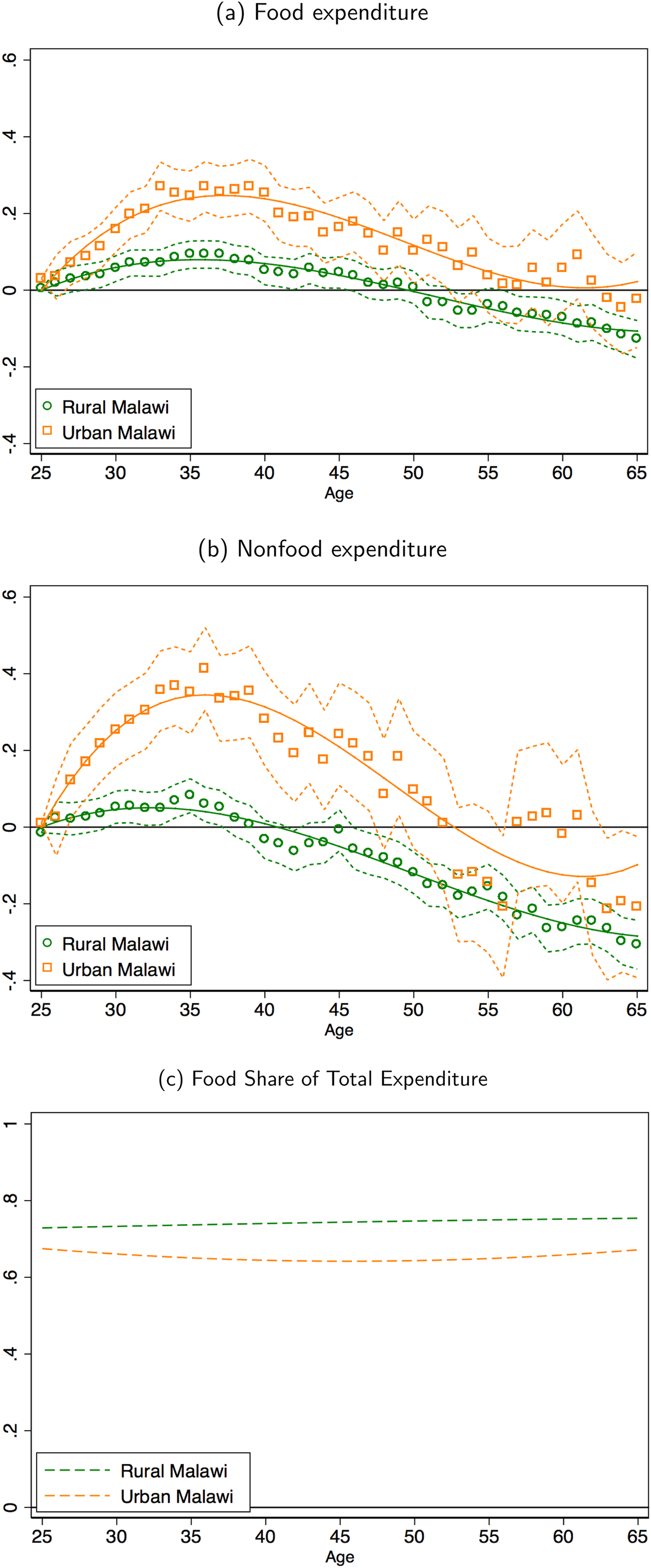
Figure 3. Lifecycle food and nonfood expenditure.
4.1.3 The role of self-farmed food
Given the role of food in explaining the smoothing of total expenditure, we now investigate food expenditure in more detail. In particular, we break down expenditure in different categories. We deconstruct adult-equivalent lifecycle behavior of food into purchases, the monetary value of self-farmed food, and received food gifts.Footnote 35
First, the only category that goes up over the lifecycle is self-farmed food [left axis, panel (a), Figure 4]. In rural areas, the monetary value of self-farmed food is 0.22 log points higher at age 65 compared to age 25. The increase in urban areas is more pronounced in old age and the monetary value of self-farmed food is 0.52 log points higher by age 65. The share of self-farmed food also increases during the lifecycle: from 38% to 48% in rural areas and from 4% to 17% in urban areas [right axis, panel (a), Figure 4].Footnote 36
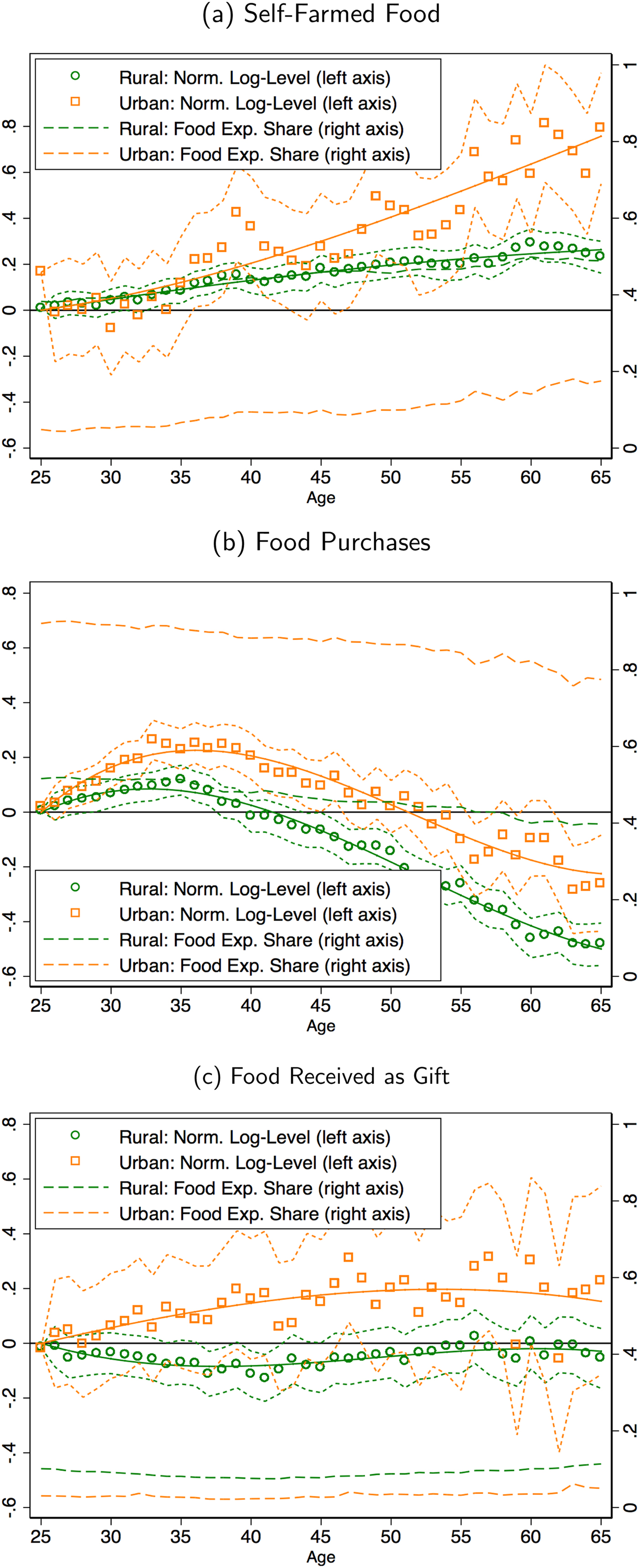
Figure 4. Deconstructing lifecycle food expenditure.
Second, food purchases show a hump that decreases substantially after peaking around ages 30–40 [left axis, panel (b), Figure 4]. The hump in food purchases is larger than that of total nondurable expenditure. The decrease is particularly strong in rural areas where the level of purchased food is below that of age 25 by age 40, and by age 65 the level is lower by −0.51 log points. In urban areas, the level of purchased food by age 65 is below that of age 25 by −0.31 log points. The share of purchased food also decreases during the lifecycle: from 52% to 40% in rural areas and from 92% to 78% in urban areas [right axis, panel (b), Figure 4].
Third, the level of food expenditure from gifted consumption in rural areas is relatively flat throughout the lifecycle [panel (c)]. In urban areas, we observe a hump shape peaking age 45 and attaining the same level at 65 as that of age 25. In neither urban nor rural areas does the share of received food gifts increase in old age. The share remains relatively stable at 10% in rural areas and 4% in urban areas.
Our decomposition of food expenditure suggests that the main mechanism to smooth food expenditure in old age is the substitution away from purchased food and into self-farmed food.Footnote 37 Our results cast doubt on two alternative traditional explanations for consumption smoothing over the lifecycle. First, the decrease in purchased food in old age together with the low ability to accumulate wealth and dissave suggests that traditional savings play a lesser role in explaining consumption smoothing mechanism for old age. To see this, we plot asset accumulation over the life cycle in terms of households net worth as well as land and livestock for rural and urban areas in Figure 5. These graphs show that wealth accumulation is low and, perhaps, more importantly, the behavior of wealth over the lifecycle suggests no sign of dissaving previously accumulated assets in old age.Footnote 38 That is, against what the standard lifecycle model predicts, net worth remains relatively constant after age 50, including land and livestock. This pattern of lifecycle accumulation of land and livestock (both farming inputs) further suggests a strategic move towards self-farming in old age which goes hand in hand with the increase in self-farming food consumption that we document. Second, the stability of food gifts over the lifecycle suggests that informal risksharing arrangements which are important against unanticipated income shocks [Townsend (Reference Townsend1994); Kinnan (Reference Kinnan2014)] do not contribute to consumption smoothing in old age.
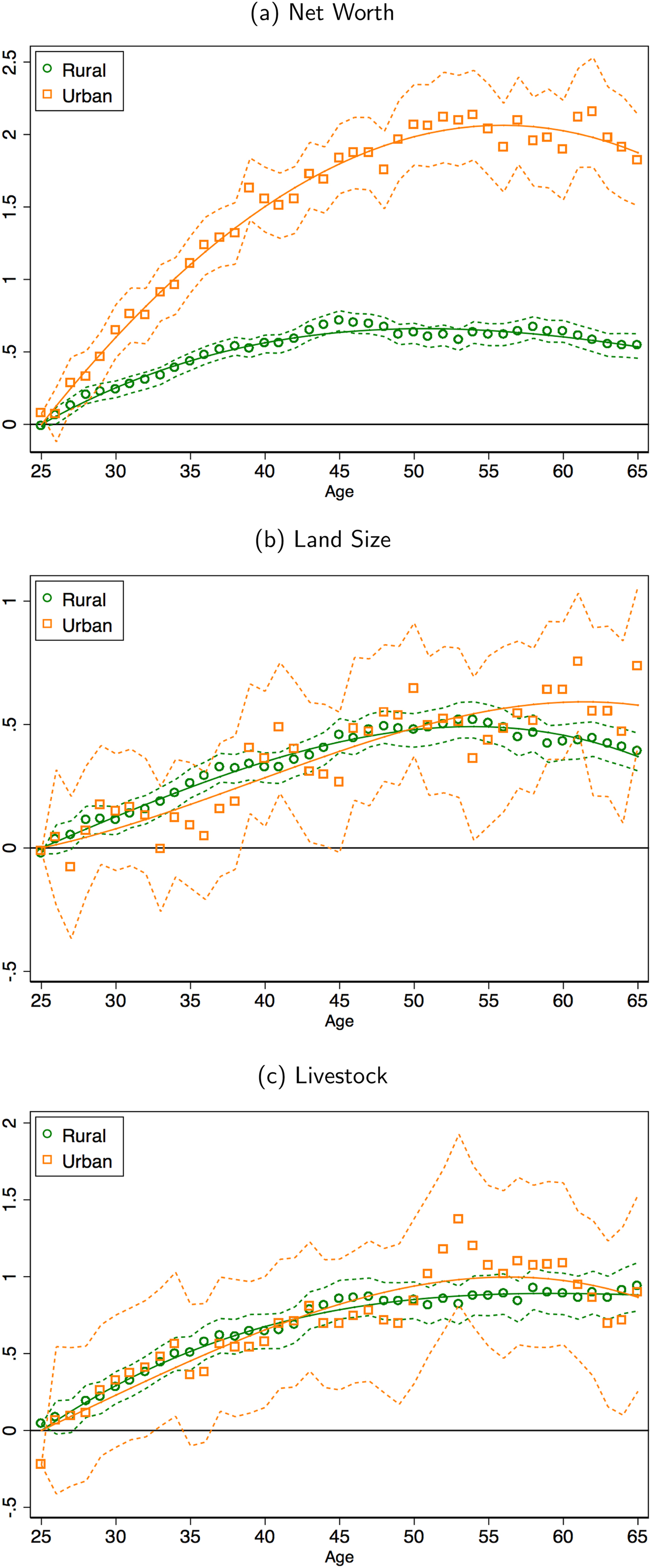
Figure 5. Lifecycle wealth.
Although suggestive, our results imply that alternative mechanisms to savings and gifts must be in place to smooth consumption across stages of life. In particular, the decline in purchases together with the stability of gifts implies that the increase in self-farming over the lifecycle that we document must be behind the observed smoothing in old age. In Section 4.3, we dig deeper into the mechanisms that sustain self-farming in old age and explore whether this consumption smoothing strategy entails costs.
4.2. Lifecycle consumption
An important aspect of lifecycle smoothing is potential differences between food expenditure and consumption measured in caloric intake [Aguiar and Hurst (Reference Aguiar and Hurst2005)]. This is particularly relevant in poor countries because food is the largest item of the consumption basket. Indeed, the “humps” estimated may simply reflect the natural changes in preferences and needs that occur during the life cycle. For example, individuals may prefer more expensive calories when they are middle-aged than when they are elderly.Footnote 39 To partly address these issues, we need to abstract from prices. In this section, we study the lifecycle behavior of total caloric intake and the quantity consumed (in kilograms) of the main staple food (e.g., maize in Malawi).
Adult equivalent food consumption, measured in terms of caloric intake, is more stable over the lifecycle than expenditure. In rural areas, caloric intake peaks in the early 30s with a deviation of 0.03 log points with respect to age 25, i.e., half the peak of food expenditure [panel (a), Figure 6]. The decline after the peak is also less pronounced for caloric intake reaching a deviation of −0.04 log points at age 65 that is half that of food expenditure. In urban areas, caloric intake peaks in the late 30s with a deviation of 0.09 log points with respect to age 25, i.e., less than half the peak of food expenditure [panel (b), Figure 6]. The decline of caloric intake after the peak is about the same as that of food expenditure, reaching a deviation of −0.06 log points at age 65. This implies that the total range of caloric intake over the lifecycle is 0.07 log points in rural areas and 0.15 log points in urban areas. Recall that for food expenditure these figures are respectively, 0.19 for rural areas and 0.29 for urban areas. That is, households smooth caloric intake twice more than food expenditure in both rural and urban areas. Note that the rural-urban divide persists with consumption. Consumption is twice as smooth in rural as in urban areas.
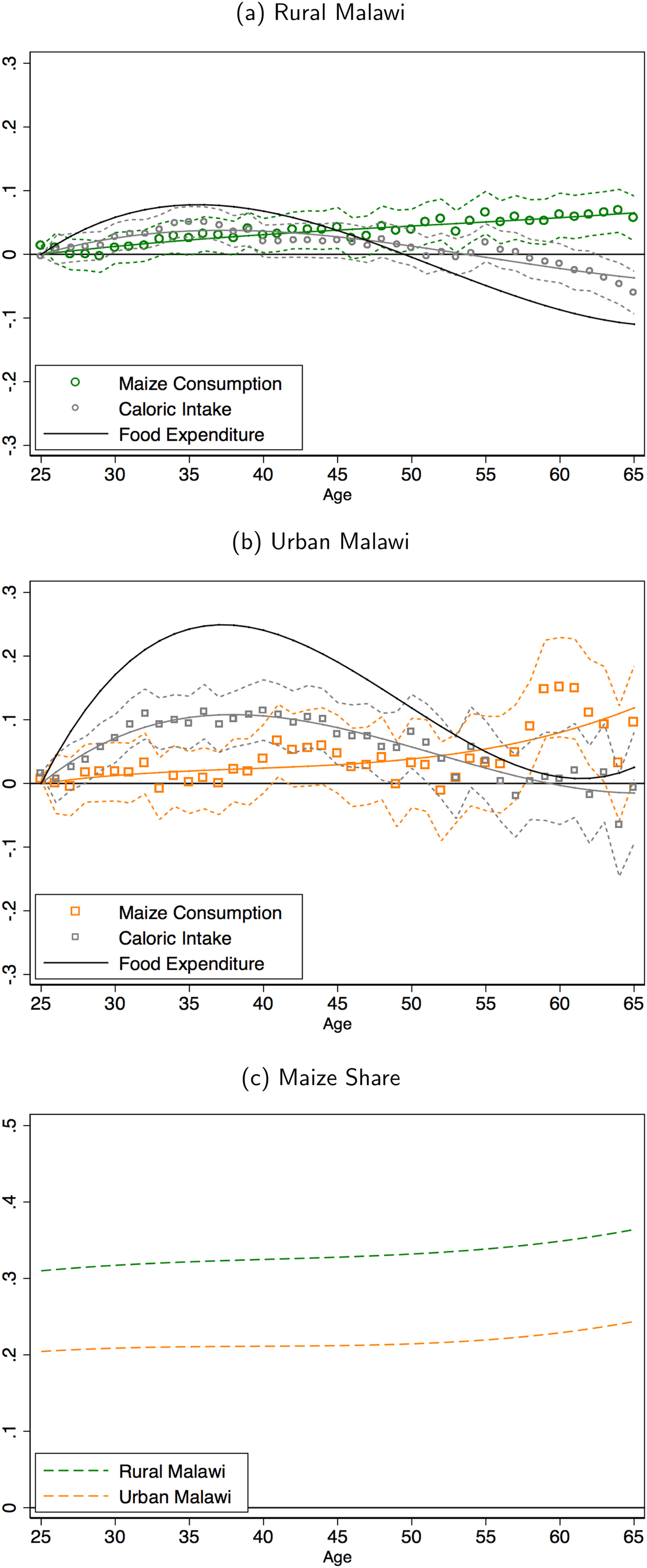
Figure 6. Lifecycle consumption vs. expenditure.
Maize is by far the most important staple food in Malawi and represents 61% of the total household caloric intake (65% in rural areas and 46% in urban areas). Such a specialization in both production and consumption in Malawi provides us with a natural and direct way to compare consumption and expenditure. We find that household maize consumption (measured in kilograms) steadily grows throughout the lifecycle, both in rural and urban areas [respectively, panel (a) and (b), Figure 6]. Indeed, Malawian households increase lifecycle maize consumption substituting away from other forms of food [panel (c), Figure 6]. This implies that the consumption of maize largely drives the smoothing of caloric intake over the lifecycle. In Section 4.3.2 we discuss what happens to the quality of food consumption.Footnote 40
To sum up, households are capable of smoothing adult-equivalent consumption through the lifecycle to a much larger extent than what measures of adult-equivalent food expenditure suggest. This result echoes the results for the United States in Aguiar and Hurst (Reference Aguiar and Hurst2005) and for Mexico in Hicks (Reference Hicks2015) that find a stable caloric intake in old age, despite a decline of food expenditure in old age. In the case of Malawi, the consumption of self-farmed maize largely drives the smoothing of caloric intake over the lifecycle but at the expense of everything else. This potentially implies negative consequences for the quality of the food consumed in households headed by the elderly.
4.3. The costs of smoothing
In the previous section, we have shown a substantial ability to smooth lifecycle consumption and expenditure in Malawi. This smoothing is characterized by an increase in self-farmed food consumption, mainly, maize. We now examine two costly consequences of this smoothing strategy.
4.3.1. More farm work and less schooling
To study how the rise of self-farmed food is sustained over the lifecycle, we explore the behavior of household hours employed in self-farming, i.e., farm work conducted on the plots cultivated by the household. We focus the discussion on rural areas, where 85% of the population lives and 77% of the rural heads engage in self-farming. Household heads work an average of 26 h per week and spend 61% of their working hours self-farming.Footnote 41 Spouses and cohabiting adult children work, respectively, 22 and 17 h per week self-farming which implies that they spend an even higher percentage of their own working time in the household farm, respectively, 93% and 89%.Footnote 42 School-age children do (on average) farmwork for 8 h a week which represents 97% of their total hours worked.Footnote 43
Consistent with self-farmed food consumption, we find that household's hours worked on self-farming in rural areas grow roughly by 0.22 log points from ages 25 to 65 [panel (a), Figure 7]. Interestingly, a decomposition of household hours worked on self-farming shows that household heads (and their spouses) increase these hours by almost only 0.1 log points from age 25 to 50, and decrease them thereafter. That is, the work of heads (and spouses) falls short in explaining the increase in household farm work. The increase in farm work is sustained by the hours that cohabiting children—both adult and school-age children—employ in self-farming. Adult children increase their hours in self-farming by 0.12 log points and school-age children by 0.20 log points [panel (c), Figure 7]. In other words, households seem to increasingly divert labor resources into self-farming over the lifecycle, a feature that is sustained by increasing the hours worked by children. Note that this increase in self-farming activities as a mechanism to provide consumption smoothing over the lifecycle is in itself a decision to smooth income—by shifting the households' income sources—over the lifecycle.Footnote 44
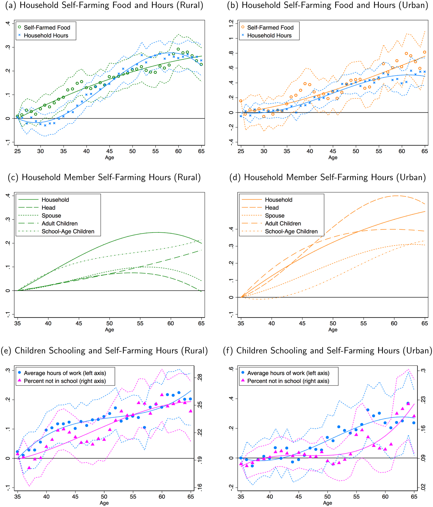
Figure 7. Self-farming hours and schooling.
This smoothing strategy has direct and costly consequences for children. We find that school-age children work more hours in households headed by the elderly and are less likely to attend school [panel (e), Figure 7].Footnote 45 To be precise, in households headed by a 65-year-old, school-age children spend (on average) 30% more hours self-farming than school-age children living in households with a 35-year-old head.Footnote 46 Further, more farm work conducted by school-age children is associated with less schooling. We find that the percentage of school-age children in a rural household not attending school increases from 19% in households with a head aged 35 to 24% for households with a head aged 65, i.e., an increase of 41%.
In Figures C.1 and C.2 in the on-line appendix, we break down the results in the above paragraph between primary (6–13) and secondary (14–18) school-age children. The number of primary school-age children not in school increases slightly over the lifecycle in rural areas, but the increase is not statistically significant. Hours worked in self-farming by primary school-age children increases over the lifecycle and this increase is statistically significant. Regarding secondary school-age children in rural areas, both the increase in hours worked in self farming and the increase in non-attendance are statistically significant. Moreover, we show in Figure C.1 and C.2 that these results are robust to excluding households with single-parents and with adopted/foster parents and focusing on households in which all children have both parents. This robustness exercise shows that our results are not due to a composition effect where older households are more likely to foster children and treat them differently [Ainsworth (Reference Ainsworth1996); Zimmerman (Reference Zimmerman2003); Case et al. (Reference Case, Paxson and Ableidinger2004); Evans and Miguel (Reference Evans and Miguel2007); Akresh (Reference Akresh2009)].Footnote 47
These results suggest a substantial loss of human capital for future generations associated with consumption smoothing achieved through self-farming. School-age children raised in households with elderly heads are less likely to attend school and have to spend more time working on the farm. There is no indication that selection among school-age children is driving these results as the result is robust to households in which all children have both parents present. These children follow their parents in their choice to cohabit with the elderly head (i.e., the grandparent). It is likely there is some selection among the adult children who cohabit with their elderly parents. Note, however, that even with selection among siblings, cohabiting adults would have been more efficiently employed elsewhere in the economy than in the subsistence sector [Gollin et al. (Reference Gollin, Lagakos and Waugh2014)].Footnote 48
4.3.2. A nutritional loss
A consumption smoothing strategy by which elderly households divert resources into self-farmed foods, mainly, maize, is likely to have negative consequences on the quality of food intake. We find that this is the case in adult equivalent nutrient intake. Consistent with a diet where maize is the staple food, households are able to smooth iron and zinc in both rural and urban areas, respectively, in panel (a) and (b) of Figure 8. In contrast, a look into vitamins shows a very different story. In rural areas, the consumption of vitamin A, B12, C, and D show a similar but even larger hump and range over the lifecycle than food expenditure. In particular, there is a substantial nutrient loss in terms of all vitamins consumption at age 65 with log deviations of −0.10 for vitamin C, −0.13 for vitamin A, −0.18 for vitamin D, and −0.19 for vitamin B12 compared with age 25 consumption [panel (c), Figure 8].Footnote 49 This loss in vitamins consumption is between two and five times that of caloric intake that is barely −0.04 log points at age 65. For the 15% of the population that lives in urban areas, the nutritional loss in old age is particularly stark for vitamin B12 and vitamin D with log deviations of, respectively, −0.37 and −0.20 compared with age 25 consumption [panel (d), Figure 8]. Interestingly, vitamin A and C grow and smooth better over the lifecycle in urban areas. Finally, macronutrients such as fat and sugar intake also drop in both rural and urban areas below the levels at age 25 [panel (e) and (f), Figure 8]. Overall, there is a clear reduction in the quality of household food intake in households with an elderly head. This is consistent with a substitution of most food items toward the consumption of the staple food, maize. Maize provides calories and iron, but not much more.Footnote 50
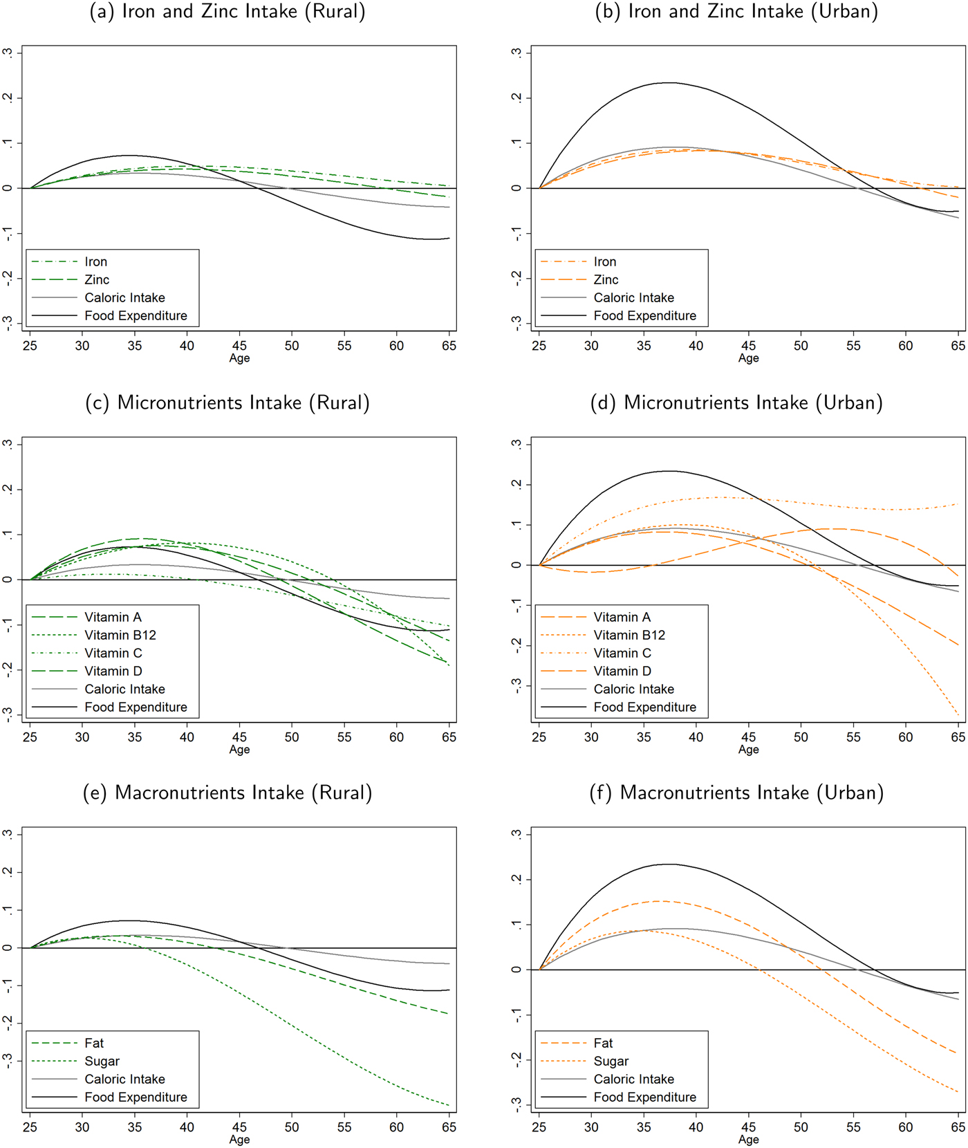
Figure 8. Quality of lifecycle consumption.
Our findings contrast with previous results for richer countries such as the United States where food quality remains stable in old age [Aguiar and Hurst (Reference Aguiar and Hurst2005)], suggesting that these results can depend on the aggregate stage of economic development. Smoothing in old age that is achieved through (dis)savings or social security systems that provide pension income (which are features of more developed economies) are likely to affect diet variety much less than smoothing strategies that rely on increasing self-farming staple food in old age.
5. Conclusion
The incentives to smooth consumption over the lifecycle are powerful. Our investigation shows that households in some of the world poorest countries are able to smooth consumption fairly well throughout the lifecycle. We find that this successful smoothing strategy is characterized by the substitution away from purchased food and into self-farmed staple food (e.g., maize in Malawi) in old age. This strategy operates through a new mechanism by which household heads cohabit with their children in order to smooth consumption by shifting labor supply (hours of family members, in particular, of their children) to self-farming. Our results provide an alternative mechanism to the standard lifecycle theory in which consumption smoothing is achieved through traditional saving methods, which can be inaccessible to the SSA populations that we study, or through food transfers across generations.
The lifecycle shift toward self-farmed food has two important costly consequences. First, school-age children are diverted away from school and toward the cultivation of self-farmed food, thus lowering education attainment and human capital accumulation. Second, the nutritional quality of the household's food consumption is substantially reduced. For example, in Malawi, a diet in which the importance of maize consumption increases over the lifecycle provides iron and zinc for individuals living with elderly heads, but not much more. Moreover, these two costs are intertwined as poor nutrition in children can lead to lower schooling [Behrman (Reference Behrman2009)].
Ultimately, our results suggest that consumption smoothing based on self-farming can provide a breeding ground for aggregate stagnation with low schooling and poor nutrition. The choice of this consumption smoothing strategy despite its costs suggests that the incentives for smoothing potentially overpower the incentives to generate economic growth in the poor countries that we study.Footnote 51 An argument that we think deserves further exploration. In this direction, the provision of alternative mechanisms to smooth consumption in old age (e.g., a higher ability to save or direct transfers to the elderly) is likely to help kick-start economic growth. Some evidence that such a policy could work can be seen in Bethencourt and Ríos-Rull (Reference Bethencourt and Ríos-Rull2009). They show—for the United States—that as the relative income of elderly widows grows relative to the income of their adult children, cohabitation is less likely. This suggests that interventions of providing pension income to the elderly in Malawi may reduce co-habitation and the costs associated with it, particularly, less schooling. We leave all these interesting questions for future research.
Supplementary material
The supplementary material for this article can be found at https://doi.org/10.1017/dem.2019.7.


