


It has been widely acknowledged that the pre-industrial distribution of landownership exerted a continuing influence on the political and economic institutions of industrializing societies across the world. Suffrage institutions historically excluded large parts of society from political influence and arguably affected long-run development through biased tax systems and public goods provision (Engerman and Sokoloff 2005). Concentration of political power in the hands of a small landed elite alongside a vast majority of the population without effective rights has been associated with the adoption of policies that mainly benefit this elite (Acemoglu, Johnson, and Robinson Reference Acemoglu, Johnson and Robinson2001, Reference Acemoglu, Johnson and Robinson2002).
The conventional wisdom regarding Prussia’s development during the second half of the nineteenth century is that the landowning elite, the Junkers, retained sufficient control over the political process to obtain political rents. According to Gerschenkron (Reference Gerschenkron1966, p. 25), due to the unequal and indirect Prussian franchise, Junkers dominated both chambers of the Prussian parliament and could thus veto legislation in the Federal Council of the German Empire. Despite several attempts to introduce an equal voting system, which were blocked by members of parliament (MPs) representing voting districts where the landed elite was concentrated, Prussia maintained a voting system that was unequal, non-secret, and indirect until the eve of WWI (Ziblatt Reference Ziblatt2008). Since 1850, members of the lower house of the Prussian parliament were elected under the so-called three-class franchise system, which translated tax payments into voting weights. Voters were grouped into three classes (Abteilungen) by total direct taxes paid. Each of the three classes represented one-third of the total direct tax revenue and received the same number of votes. Classes were filled with voters ranked according to their tax payments, starting from the highest, adding taxpayers until one-third of the total tax base was reached, thereby allocating less than 5 percent of voters into the first class, on average.
By tying voting power to economic power, the system arguably produced policies tailored to fit the landed nobility.Footnote 1 German economic historians widely agree that the franchise system was designed to “generate Conservative votes,”Footnote 2 and thereby produced (socio-) economic policies favored by agrarian elites (see, e.g., Nipperdey Reference Nipperdey1992, p. 86; Clark Reference Clark2006, pp. 560–61). Kühne (Reference Kühne1994a, p. 25) stresses that the system was “the bulwark of reactionary Prussianism par excellence.”Footnote 3 Indeed, the Prussian parliament was firmly regressive in so far as Social Democrats were not able to win any mandates until 1908. Despite this univocal assessment, the question of whether the unequal distribution of voting rights in Prussia produced conservative policies is ultimately an empirical one and has not been answered thus far.
This paper fills this gap and investigates how the three-class franchise contributed to the adoption of liberal or conservative (socio-)economic policies by the Prussian parliament. We find that MPs from constituencies with higher vote inequality, that is, where a small number of affluent voters holds a large share of the political power, vote significantly more for liberal policies. Crucially, our result of a link between vote inequality and more liberal voting holds controlling for landownership inequality, which in itself generates more conservative voting, in line with earlier claims that landed elites protected their own interests (Gerschenkron Reference Gerschenkron1966).
Post-1848 German liberalism catered to a relatively small group of bourgeois voters that advocated low taxes and free-market capitalism (Gall Reference Gall1975; Kurlander Reference Kurlander and Jefferies2015). In fact, Gross (Reference Gross2004, p. 22) summarizes the vision of German liberals as seeking progressive development toward modern rationalism, bourgeois individualism, high industrialization, free-market capitalism, and the unified nation-state. With national unity (excluding Austria) and the German constitution in 1871, central goals of liberalism had been achieved, including progressive legislation such as the penal code, the commercial code, the reform of the monetary system, and the Prussian county ordinance. The subsequent relative decline of the popularity of liberalism coincided with a period of economic stagnation (Langewiesche Reference Langewiesche and Martel1992). In the 1880s and 1890s, liberals aimed to address the looming social challenges of rapid industrialization and the demise of the working class by adopting social liberalism, a form of liberalism that opposed governmental social policy and supported “self-help” instead of “state-help” (Kurlander Reference Kurlander and Jefferies2015). Advancing public education and improving the urban infrastructure became central instruments in their strive for a liberal society (Langewiesche 1990; Palmowski Reference Palmowski1999).
In the Prussian parliament, liberal and conservative views differed on many issues. We illustrate some of the divides of the time by inspecting five salient debates in which liberals opposed tuition fees in public primary schools, supported decentralization of administrative power, opposed nationalization of railroads, supported tax exemptions for income from capital investments, and supported the construction of a canal that arguably increased competition in East Elbian grain markets.
We capture the (socio-)economic orientation of policies by measuring the political orientation of MPs using the universe of 329 roll call votes (RCVs) from the Prussian House of Representatives in the period of 1867–1903. We apply Poole’s (Reference Poole2000) optimal classification (OC) method, described in detail later, to measure two salient dimensions of MPs’ political orientation: their liberal or conservative economic orientation and their secular or religious orientation. The start year is chosen because in January 1867 Prussia reached its maximum extension after incorporating Schleswig-Holstein. The choice of the end year is due to the fact that, from the election period 20 (1904–1908), there was a change in the procedure to elect MPs, and in 1906 a range of constituencies were split. Our period of analysis is characterized by the rapid industrialization of the economy and by the secularization of society in Prussia and the German Empire more broadly.Footnote 4
The results are robust to the inclusion of a sizable set of constituency-level control variables capturing regional development and thereby the political preferences of the median citizen. Complementing the analysis with biographical information of MPs, we also inspect whether voting was biased toward MPs’ personal agendas. The inclusion of both sets of variables does not change our main qualitative findings.
Furthermore, we control for party affiliation. Of course, since parties are collectives of like-minded people, party affiliation captures a lot of the variation in political orientation of MPs. But since parties did not exercise complete control over MP voting behavior, there is sufficient within-party variation in political orientation that our main results hold conditional on party affiliation.
Despite the fact that our broad set of control variables explains a substantial amount of variation in the political orientation of MPs, we discuss remaining endogeneity concerns related to omitted variable bias. As we explain in more detail later, the allocation of voters to classes reflects local thresholds between terciles of the tax base that are arbitrary from a national perspective. In locations with a large number of high-income earners, voters with high incomes are more likely to be allocated to lower classes than elsewhere. Using this insight, in a robustness check, we further aim to mitigate endogeneity concerns by using the share of voters in the first class as an instrumental variable (IV) for vote inequality. Resulting IV estimates confirm the link between vote inequality and liberal orientation.
In placebo tests, we inspect whether the “secular-religious” dimension of political orientation responds to vote inequality. Conflicts between Protestants and Catholics that culminated in the secularist policies of the Kulturkampf (“culture struggle”) era in the 1870s transcended class structures and should not be reflected in the distribution of voting power. Indeed, we find that vote inequality does not predict for which type of cultural policies MPs vote.
What explains our results? The three-class franchise was designed when industrialization was in its infancy. The rise of large-scale industry in late nineteenth-century Prussia increased earnings and tax contributions of industrialists. This development resulted in a stronger income dispersion and therefore in higher vote inequality in industrial regions (Kuznets Reference Kuznets1955; Bartels Reference Bartels2019) than in agricultural regions where the income of landowners remained largely unchanged. As a consequence, the highly unequal distribution of individuals across voting classes in industrial regions created a small and homogeneous first class, which was able to coordinate on electoral delegates during primary elections (Urwahlen) and to influence the selection of their favorite MP, who would support liberal policies, as our results show. Our result of an effect of vote inequality on liberal orientation of MPs holds for Prussia in general. In line with our expectations, we find that this effect is particularly pronounced in regions with a high share of large firms whose owners would benefit the most from liberal economic policies.
Our findings are in line with a recent literature debating the role of elites in the process of modernization and democratization. This literature presents results that are broadly consistent with the idea that elites prefer “liberal” policies if those are in their own interest.Footnote 5 For example, Ashraf et al. (Reference Ashraf, Francesco, Oded, Boris and Hornung2017) argue that capital-owning elites in industrializing Prussia granted more freedom to the masses to incentivize their labor effort. In Tsarist Russia, liberal nobles cooperated with the peasantry to expand public goods provision (Nafziger Reference Nafziger2011). In nineteenth-century Sweden, a suffrage reform shifted voting power from landed elites to industrialists, resulting in higher investments in railways and structural change (Hinnerich, Lindgren, and Pettersson-Lidbom Reference Hinnerich, Lindgren and Pettersson-Lidbom2017). In Revolutionary France, the enlightened elite supported more “liberal” education policies (Squicciarini and Voigtländer 2016).
We also contribute to a large literature that uses RCVs to study the orientation of historical parliaments (see, e.g., Schonhardt-Bailey Reference Schonhardt-Bailey1998; Rosenthal and Voeten Reference Rosenthal and Voeten2004; Heckelman and Dougherty 2013). We are not aware of work that systematically analyzes RCVs from the Prussian House of Representatives. However, inspecting a period that strongly overlaps with ours, Häge (Reference Häge2019) provides a descriptive analysis of the policy space across different Reichstag legislatures during the Bismarck era in the German Empire.Footnote 6 While their orientation shows similarities, the two parliaments differ in their franchise system. Thus, discrepancies in dimensionality and party affiliation could be the outcome of a fundamentally different political process. In addition, our paper focuses on explaining rather than describing the orientation of parliament.
Earlier work that tried to explain voting behavior in the Prussian House of Representatives has so far focused on selected RCVs debating important issues. Ziblatt (Reference Ziblatt2008) analyzed one RCV seeking to abolish the three-class franchise in 1912 and finds higher landownership inequality but not income inequality to be associated with voting in favor of preserving the three-class system.Footnote 7 Mares and Queralt (Reference Mares and Queralt2014) analyze one RCV on the introduction of a Prussian income tax system in 1891, showing that higher landownership inequality is associated with voting for the adoption of an income tax that disproportionately burdened the industrialists.Footnote 8
Thus, on the data front, we go beyond previous work by using the universe of RCVs in the Prussian House of Representatives during 1867–1903. We consider this data work a major contribution for several reasons: First, future research will be able to analyze any or all of the RCVs not analyzed in earlier single-RCV studies. Second, future research will be able to use previously unavailable measures of political orientation for Prussia derived with the OC method based on the universe of RCVs.
HISTORICAL CONTEXT
In 1848/1849, Prussia introduced a bicameral parliament, with an appointed House of Lords (Herrenhaus) and an elected House of Representatives (Abgeordnetenhaus). The constitution, imposed by the King, stipulated that the lower chamber was elected by male citizens aged 24 or older who had paid taxes in the preceding year. Additionally, the exclusion of women and of those not paying taxes is a form of unequal voting, which was very common until the early twentieth century. However, in Prussia, voters were allocated to three classes reflecting terciles of the total direct tax base. Votes were effectively weighted in proportion to payments of direct taxes (class-tax, classified income tax, real estate and property tax, and business tax): the upper tercile of tax payments had as many votes as the middle tercile and the lower tercile. On average, first-class voters had about 17.5 times the number of votes of third-class voters, even stronger inequality at the local ward (Urwahlbezirk) level. In the extreme, a single taxpayer who paid one-third or more of direct taxes in a ward would have as many votes as all of the taxpayers in the lower tercile combined.Footnote 9
The thresholds for allocating voters into the three classes according to their tax payments were determined at the municipality level.Footnote 10 Municipalities with more than 1,750 inhabitants were subdivided into wards but maintained the municipality-level tax thresholds.
The mayor was responsible for the division into wards, frequently leading to gerrymandering (Kühne Reference Kühne1994a; Richter Reference Richter2017). In cases where social stratification led to sorting into city quarters, the first and second class remained unpopulated in poorer wards, whereas the first class was populated by many voters in richer wards, reducing individual voting power in wealthy city quarters.Footnote 11
Elections proceeded in two stages: in stage one, the primary elections (Urwahlen), voters elected electoral delegates (Wahlmänner). In stage two, the electoral delegates elected the members of the House of Representatives. Stage one was voting by a show of hands, in other words, non-secret, and took place at the level of wards.Footnote 12 Each class in a ward elected the same number of delegates, ranging between 3 and 6 per ward, one per 250 inhabitants (according to the last census). At the second stage, electoral delegates from all wards in an electoral constituency met to elect between one and three MPs, depending on its population size. The three-class franchise was frequently disputed but persisted in parallel with the equal voting system of the Imperial Diet, the Reichstag, until 1913.
The Political Landscape
The Prussian party landscape stabilized during the early periods of our analysis. Political fractions and parties formed during the 1860s, and gained relevance after German Unification in 1871, when the German Reichstag was established.Footnote 13
Drawing on biographical information from Kühne (Reference Kühne1994b), we report the party affiliation of MPs in Table 1.Footnote 14 The table depicts an aggregate number of 3,658 MP-by-period observations of party affiliation between 1867 and 1903. A range of smaller factions were represented in parliament. Following the detailed discussion in Treue (Reference Treue1975), we classify members of smaller factions into larger party groups as indicated in Columns (2) and (3). This leaves us with six main parties that were active during our period of analysis (and the residual category “Other” (1.35 percent of observations)).
Table 1 PARTY AFFILIATION FREQUENCY
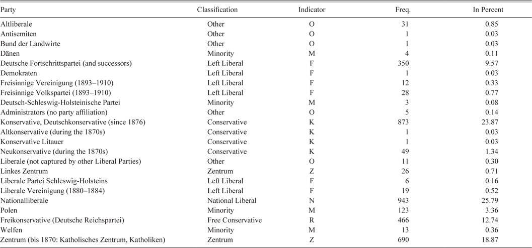
Notes: This table reports the party affiliation of all 3,658 MP-by-period observations whose votes were scalable. Column Party depicts the original party assignment according to Kühne (Reference Kühne1994b). Cases in which party affiliation was uncertain were coded according to the most likely party affiliation. Column Classification consolidates smaller parties with similar platforms. Column Indicator lists a party code used in graphical presentation of the policy space. Columns Freq. and In Percent show the frequency and share of party affiliation.
Source: See Kühne (Reference Kühne1994b) and Online Appendix A.
Parties offered a wide spectrum of political views, which we discuss in more detail in Online Appendix A.1.Footnote 15 However, due to the inequalities embedded in the franchise system, parties addressing social issues and redistribution such as the Socialist Workers’ Party (later Sozialdemokratische Partei Deutschlands (SPD)) did not manage to obtain any seats in parliament until 1908.Footnote 16
For the purpose of our analysis that focuses on positions of MPs, it is important to note that party discipline was far from perfect. In fact, as we will show, MPs often deviated from the party line, a key feature permitting analysis of MPs’ political orientation.
Roll Call Voting
The Prussian constitution of 1850 stipulates in article 64 that the King and each of the chambers have the right to introduce bills. In the House of Representatives, legislative proposals can be introduced by the president of the chamber or by groups of at least ten MPs. To vote, the majority of members of the chamber must be present. Proposals are voted on by absolute majority. To adopt a law, all three sides (King and both chambers) must agree, so they are fully equal in the legislative process.
Voting in the House of Representatives took several forms. When the majority on an issue was clear-cut, a count based on standing or sitting MPs established the result. RCVs were triggered in one of two ways: (1) on request of at least 50 MPs (Plate 1903, p. 187; §61 GO) and (2) with a majority of less than 15 votes, a roll call could be requested without further support/signatures (Plate 1903, p. 187; §58 GO). From 13 February 1875, some roll call votes were replaced by a division of the assembly (Hammelsprung).Footnote 17 This reform likely explains why the number of roll call votes declined after 1875 (see Table A.1 in the Online Appendix). The absolute majority decided all votes. Abstentions were typically not included in the calculation of the majority.Footnote 18
Since RCVs were only called on close and/or contentious issues, they are likely to be quite selective (Carrubba et al. 2006). This has advantages and disadvantages: RCVs are associated with highly important issues, which is a clear upside for our analysis. On the other hand, party discipline tends to be enforced more strongly in RCVs, at least in modern parliaments (Yordanova and Mühlböck Reference Yordanova and Mühlböck2015). If that was true also in historic parliaments, and if we could observe all votes in the Prussian Parliament, the actual variation in political orientation across MPs would likely be larger than what we observe using only RCVs. However, our analysis shows that there is substantial variation in political orientation within parties, in other words, de facto party discipline is far from perfect. This has important implications for our analysis because we capture meaningful variation in political orientation above and beyond what is predicted by party membership.
CONCEPTUAL FRAMEWORK
The three-class franchise was created at a time when industrialization was still in its infancy and income inequality was relatively low. Large landowners paid a sufficient amount of taxes to populate the first two classes, despite the fact that they enjoyed a range of tax exemptions and paid little taxes on land—their main source of income. Due to the rapid rise of large-scale industry in the second half of the century, industrialists started to obtain high returns to capital investment and incurred an increasing share of the total tax base (Bartels Reference Bartels2019). In industrializing regions, this development lifted the new industrial elites into the first two classes, where they crowded out parts of the traditional elites. Thus, the rise of industry created an unforeseen regional concentration of high incomes and thereby a higher level of vote inequality in industrializing regions while vote inequality in agricultural regions was less affected. This description is in line with the developments first observed by Kuznets (Reference Kuznets1955) who also relied on Prussian income data (also, see Grant Reference Grant2002; Bartels Reference Bartels2019).
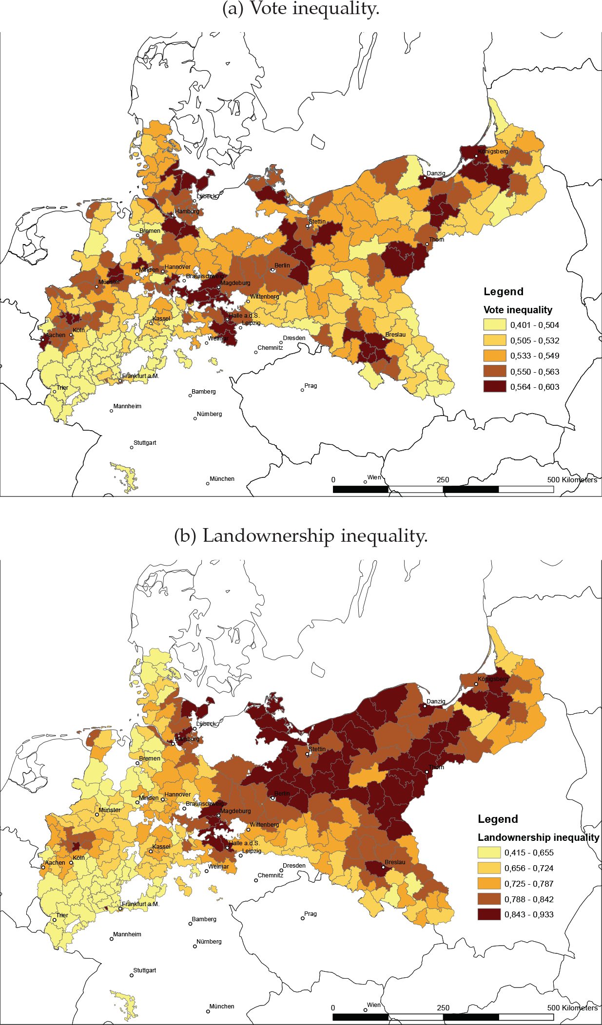
Figures 1(a) and 1(b) depict the spatial variation of vote inequality and landownership inequality across Prussia. Regions with high levels of vote inequality, as measured by a Gini coefficient across franchise classes, can be found throughout Prussia, especially in more urban and industrial locations.Footnote 19 The spatial distribution of landownership inequality, as measured by a Gini coefficient across farm size classes, shows that landownership inequality concentrates in the more rural eastern provinces. A comparison of the two maps visually confirms our previously noted interpretation that the mechanics of the franchise system may have provided political rents to an industrial elite and were not exclusively captured by the agrarian elite.

Figure 1 SPATIAL VARIATION IN INEQUALITIES IN PRUSSIA
Notes: The figure shows the spatial distribution of vote inequality and landownership inequality. Vote inequality is a Gini coefficient calculated using the county-level number of voters in each class in the three-class franchise system of 1893 assuming that the tax burden of each class amounts to exactly one-third. Landownership inequality is a Gini coefficient calculated using the county-level number of farms with arable land by size-class (up to 1 hectare, 1 to 2 ha, 2 to 10 ha, 10 to 50 ha, 50 to 100 ha, and more than 100 ha) in 1882.
Source: See Online Appendix C for data sources.
DIVERGING INTERESTS
We assume that the new concentration of industrialists at the top of the income distribution led to the creation of a small first (and likely second) class of voters whose interests were best served by policies that allowed them to explore economic opportunities arising from decentralization, improved transport infrastructure, or tax exemptions for capital gains.Footnote 20 Such policies were firmly supported by MPs in parties self-identifying as “liberal” in their name, which propagated liberal economic policies, stressed the need for (domestic) competition, and supported the separation of church and state.
On the other hand, we assume that large landowners predominantly favor policies that protect their (socio-)economic status. In rural regions with little competition over entry into the upper classes, political preferences in the first and second class therefore should remain conservative. Higher levels of landownership concentration may reflect higher demand for social control due to a higher risk of expropriation for the elite (Weber Reference Weber1917; de Tocqueville Reference de Tocqueville1856). Since landowners rely on an immobile factor of production, they prefer conservative policies that sustain inequality (Acemoglu and Robinson Reference Acemoglu and Robinson2000; Boix Reference Boix2003).
So far, we have highlighted the polar cases of industrialists and landowners, as if their interests were ideal points in a spectrum.Footnote 21 However, industrialization in agricultural regions may have similarly increased heterogeneity in political preferences. Any heterogeneity of interests within the first class of voters should lead to the election of less conservative MPs, even in initially purely agricultural areas.
FROM GROUP INTERESTS TO MP ORIENTATION
In the two-stage election system, where each class voted for electoral delegates who in turn elected MPs, the electoral college commands particular power. Kühne (Reference Kühne1994a, pp. 51–52) suggests that electoral delegates served as intermediaries between the electorate and MPs. Because the socio-economic background of delegates and first-class voters overlapped, the elite often succeed in electing their desired MP. Furthermore, a more concentrated economic elite will find it easier to coordinate on and influence electoral delegates, and in extension local MPs because smaller groups of homogeneous voters will find it easier to coordinate on outcomes.Footnote 22 Coordination costs are likely to be the lowest in the industrial urban areas because of higher population density, better transport infrastructure, and low information costs (Kühne Reference Kühne1994a, pp. 51–52). We therefore expect a stronger link between vote inequality and liberal voting in areas with industrial elites.
But there is another reason why the interests of industrial elites may have translated into a majority for liberal MPs in their constituencies: a strategic complementary between the interests of first- and third-class voters. It is often argued that during the second phase of industrialization, roughly corresponding to our period of analysis, industrial elites may have formed a strategic coalition with the third class to support policies that are mutually beneficial for capitalists and workers (also, see Galor and Moav Reference Galor and Moav2006; Doepke and Zilibotti Reference Doepke and Zilibotti2008; Llavador and Oxoby Reference Llavador and Oxoby2005), for example, free public schooling and freedom of occupational choice that benefited both industrialists and workers.
In summary, we expect higher vote inequality to be associated with the election of MPs with more liberal viewpoints, especially in districts with large-scale industry.
Results from Selected RCVs
Before we analyze the relationship between aggregate measures of political orientation and vote inequality, we present examples of specific roll calls in which vote inequality explains the voting behavior of MPs.Footnote 23 For this regression analysis, we select five RCVs that meet the following criteria: substantial relevance for the Prussian economy, substantial divide between liberal and conservative positions, sufficiently narrow margin so that the result may be altered by reasonable changes in inequality, and broad coverage of topics and election periods.
Table 2 presents results from regressions of an indicator variable (yea/nay) on a Gini index of vote inequality for each of the five RCVs.Footnote 24 Results reflect a linear probability model where vote inequality affects the probability to vote “yea.” In each RCV, we determine whether a “yea” vote reflects liberal or conservative position by the fact that the majority of MPs from conservative or liberal parties voted for the position (see top of Table 2 for positions). Throughout, we control for a Gini index of landownership inequality, the most important aspect of the political economy according to the literature.Footnote 25 A more detailed summary of the parliamentary debates surrounding each RCV can be found in Online Appendix B.
Table 2 RESULTS FOR SELECTED ROLL CALL VOTES

* = Significant at the 10% level.
** = Significant at the 5% level.
*** = Significant at the 1% level.
Notes: This table reports results from linear probability models estimated for five individual RCVs. The roll calls are nr. 44 in election period 10 (Column (1)), nr. 65 in election period 10 (Column (2)), nr. 1 in election period 14 (Column (3)), nr. 10 in election period 17 (Column (4)), and nr. 6 in election period 19 (Column (5)). The binary dependent variable assumes the value one for yea and the value zero for nay votes. Vote inequality (sd) and landownership inequality (sd) are standardized with zero mean and a standard deviation of one. We denote the conservative (C) and liberal (L) position at the top of the table. A position is coded as conservative if the majority of MPs from the conservative parties voted for it, and vice versa. Standard errors, clustered at the constituency level, in parentheses.
Source: See Online Appendix C for data sources.
Across the five roll calls, we find that MPs from districts with a higher vote inequality have a higher probability of voting for the liberal position. Column (1) shows results from a RCV on the King’s bill to re-introduce school tuition fees. Since 1850, the Prussian constitution stipulated that public primary schooling was tuition free so that municipalities were required to finance schooling from taxation or other local sources. In 1869, the King proposed to revoke free tuition and was defeated by a liberal majority.
Column (2) shows results from a RCV within the debate about the major administrative reform of 1872 (Kreisordnung) that effectively ended police authority of the landed nobility. The amendment to the bill, introduced by a liberal MP, proposed that the newly introduced role of a public official (Amtshauptmann) should be filled following a selection by the local administration instead of an appointment by the King. This amendment about the decentralization of power passed with a liberal majority.
Column (3) shows results from a RCV on section 1 of the Trade Ministry’s bill that allowed the state to buy private railroad companies. The bill passed with a conservative majority and led to the nationalization of railroads in 1880. In Table B.1 in the Online Appendix, we show that vote inequality is significantly associated with voting against the bill once a larger set of control variables is included.
Column (4) shows the results from a RCV in the context of the debate about the famous income tax reform of 1891 (Hill Reference Hill1892). MPs voted on an amendment to section 16 of the bill regarding the taxation of income from investment in joint stock companies (e.g., dividends). This conservative amendment requesting a 3.5 percent deduction passed whereas a competing liberal amendment requesting a 4 percent deduction was defeated by a conservative majority.
Column (5) shows results from a RCV on a proposal to construct the Dortmund-Rhine segment of a canal connecting the rivers Rhine and Elbe, introduced by the Kaiser in 1899. Conservatives opposed the canal construction and defeated the bill because it would be detrimental to agrarian interest and would foster the import of cheap grain from the United States.
The findings allow us to discuss a thought experiment, in which we can understand how policies would have changed if vote inequality had been different (ceteris paribus). The results imply that when increasing vote inequality by one standard deviation (0.039 Gini points), the probability of voting for the liberal position increases by up to 20 percent. In two out of five RCVs such a change in inequality would have tipped the balance towards adopting the more liberal policy, in two cases the liberal majority would have been even larger, and in one case the result would remain unchanged.
MODEL AND DATA
To estimate the relationship between the political orientation of MPs and the vote inequality in their electoral constituency, we generate a dataset in which the unit of observation is an MP, or more precisely, MP-by-constituency. The reason for the subtle distinction is that a small number of MPs (104 cases) represent different constituencies over their career.Footnote 26 Our results are robust to using MPs who represent the same district throughout their career. We employ the following standard OLS framework:
 $${PolI{d_{ic}} = \alpha + \beta VoteIne{q_c} + \gamma X_c^{'} + \zeta Z_i^{'} + {\varepsilon _{ic}},}$$
where Pol Id ic constitutes a measure of political orientation of an MP i in constituency c. We use the OC algorithm (described in the next section) to construct continuously valued scores describing the voting behavior of MPs across all RCVs in which they participate. In fact, the OC algorithm will give us two OC scores, one capturing a liberal-conservative dimension, and one capturing a secular-religious dimension.Footnote 27 Vote Ineq c is our measure of vote inequality, calculated from the distribution of voters across the three classes. ${X_c^{'}}$
is a vector of constituency-level characteristics and
${X_c^{'}}$
is a vector of constituency-level characteristics and ${Z_i^{'}}$
is a vector of individual-level MP characteristics.
${Z_i^{'}}$
is a vector of individual-level MP characteristics.
Vote Inequality
Vote inequality is a Gini coefficient calculated from the distribution of voters across the three classes. Using the fact that each class contributed exactly one-third to the tax base, we calculate the Gini coefficient based on the number of voters in each class. Notice that vote inequality assigns the same power to each voter in the same class so that we do not require information about the complete, individual-level tax contributions in a constituency.Footnote 28
An individual qualified for the first class by crossing a threshold that was determined by last year’s tax payments of all voters in a municipality. The threshold is therefore determined by local conditions and not by a national classification. This consideration helps to alleviate concerns regarding endogeneity in vote inequality. The classification of voters is strongly affected by the individual with the highest income in a municipality, leading to extreme heterogeneity in the threshold determining inclusion in the first class.
Two examples may clarify the arbitrary nature of classification as discussed by contemporaries (Königlich Preußisches Statistisches Bureau 1861–1904, vol. 2, p. 109). In the election of 1861, in a ward in the county Schleiden (province Rheinland) each of the three voters with the highest tax contributions paid 270 thalers.Footnote 29 Two of them were allocated to the first class whereas the third was allocated to the second class,Footnote 30 where he had to share his vote with ten other taxpayers who jointly paid only 260 thalers in taxes. In a ward in the county Belgard (province Pomerania), the first class was populated by two voters paying 364 and 237 thalers in taxes, respectively, the second class was populated by another two voters paying 213 and 189 thalers in taxes, while the third class was populated by 160 voters with one paying 102 thalers and the remaining 159 voters combined paying 396 thalers in total. These examples show that the local economic elite did not, by definition, end up being eligible for voting in the first class. Put differently, small differences in income at the top could move individuals across classes, with substantial consequences for individual voting weights and power.
Across Prussia, on average, the threshold to become a first-class voter was a payment of 56 thalers in taxes. However, regional variation was extreme: the minimum threshold was 7 and the maximum threshold was 12,496 thalers. If an individual taxpayer contributed more than half of the total local tax base, the second class even remained unpopulated. Given that the local distribution of incomes was decisive, variation in residential location of high-income earners led to huge heterogeneity, especially in urban areas. Before a reform in 1891, municipalities first determined tax payment thresholds based on the city-wide population of voters, before subsequently breaking the electorate into wards. In wards with many high-income voters, the first class was crowded, leading to a relative devaluation of a vote. In poor wards, the first and sometimes even the second class remained empty if none of the voters crossed the city-wide threshold.
The previous examples imply that there is strong heterogeneity in the distribution of voters across classes and that the allocation of voters to classes is beyond the power of the individual. In our standard regression framework, we aim to exclude remaining systematic heterogeneity by conditioning on a substantial set of control variables. In a robustness check, we use an IV approach that exploits heterogeneity in the size of the first class, exploiting the fact—described previously—that the richest individual’s income was decisive for its size.
The earliest available measure of vote inequality for all constituencies of post-1866 Prussia is from 1893 and reported in Königlich Preußisches Statistisches Bureau (1864–1905, vol. 17).Footnote 31 Our analysis will test robustness of the results using the distribution of voters across classes from the election of 1861. These data are less prone to potential reverse causality but are unavailable for the new provinces annexed by Prussia after 1866, that means we lose more than 350 MPs.
Constituency Characteristics
Constituency-level control variables are aggregated from county-level data provided by Galloway (Reference Galloway2007) and iPEHD (Becker et al. Reference Becker, Francesco, Erik and Woessmann2014). Electoral constituencies comprised at least one, but typically several (administrative) counties (Kreise). Put differently, the approximately 500 Prussian counties are nested in 256 electoral constituencies, allowing us to map aggregated county-level census data to MPs representing these constituencies.Footnote 32 Table C.1 in Online Appendix C presents summary statistics.
Following the literature (Lehmann Reference Lehmann2010b; Mares and Queralt Reference Mares and Queralt2014; Ziblatt Reference Ziblatt2008), we include a set of standard explanatory variables for MP voting behavior in the Prussian House of Representatives in our vector of constituency characteristics.
The most important control variable is landownership inequality capturing Gerschenkron’s idea of a link between the interests of large landowners and conservative voting.Footnote 33
Other control variables include the industrial employment share, the urbanization rate, the share of Protestants, the linguistic fractionalization, the share of the population that lives in their municipality of birth, as well as the literacy rate to capture heterogeneity in the available stock of human capital.Footnote 34 These indicators measure differences in development, cultural heterogeneity, and structural differences across regions.
The period under analysis is a critical juncture in the transition from agriculture to industry. At the beginning of the period, slightly less than half of the population was based in agriculture. At the end, agricultural employment made up merely one-third of the labor force. However, these structural changes may be an outcome of the political process and therefore prone to concerns of reverse causality. Thus, in our regressions we include variables that are measured closest to the starting point of our analysis in 1867.Footnote 35 If an MP represents the average individual in his constituency, we expect local conditions to explain a large part of the variation of MPs’ voting behavior. However, if MPs represent the local elite but also act in their own interest, individual characteristics may explain a lot of the variation. We can probe this by also controlling for MP characteristics.
MP Characteristics
MP characteristics drawn from Kühne (Reference Kühne1994b) vary at the individual level and can be broadly divided into biographic and political characteristics. Table C.2 in Online Appendix C presents summary statistics.
BIOGRAPHIC CHARACTERISTICS OF MPS
Biographic characteristics include the occupation of an MP as reported in the parliamentary minutes. We coded occupations to match the following six categories: public administration, clergy, industry, agriculture, education, and services.Footnote 36 Roughly one-third (789) of the MPs in the data set report agriculture, in other words, landownership, as their main occupation. Landowners have a higher probability of being affiliated with conservative parties.Footnote 37 On the other hand, industrialists predominantly select into liberal parties.Footnote 38
The religious denomination of MPs roughly reflects the distribution within the population. In 1880, the population of the average Prussian constituency was composed of 67.2 percent Protestants, 31.4 percent Catholics, and 1.1 percent Jews. Protestants are slightly over-represented in parliament, while Catholics and Jews are slightly under-represented.Footnote 39 Two-thirds of the Catholic MPs are affiliated with the Centre party and the Polish minority party. We expect them to lean towards policies that support a strong position of the church. Additional attributes that are available from MP biographies include nobility status, academic titles, residence in the electoral constituency, and retirement status.Footnote 40
POLITICAL CHARACTERISTICS OF MPS
Further variables capture the parliamentary engagement of an MP and the context in which he was elected. RCV participation measures the share of the total RCVs in a period in which the MP participated.Footnote 41 The electoral margin captures the strength of the mandate and whether the MP seat was strongly contested.Footnote 42 The electoral turnout captures the level of representation (see, e.g., Jackman Reference Jackman1987).Footnote 43 The count of the number of MPs to be elected in the constituency captures electoral competition.Footnote 44
In a robustness test, we include measures of party affiliation as control variables. These are not a regressors like any others: by virtue of parties’ ability to draw like-minded representatives to stand for them, we expect party affiliation to absorb a substantial part of the variation in OC scores.
MEASURING POLITICAL ORIENTATION USING OPTIMAL CLASSIFICATION
To understand whether the franchise biased parliamentary voting patterns, we inspect MPs’ overall voting behavior instead of voting in single roll calls or changes in voting behavior over time.Footnote 45 This requires us to classify all votes into categories that reflect a political orientation. Manually classifying votes from 329 roll calls into liberal and conservative (or into secular and religious) leanings is a task that would be prone to many arbitrary decisions.
Simply reading minutes of parliamentary debates preceding RCVs, we could gain a nuanced impression of speakers’ positions but still incorrectly classify MP positions because debates do not reveal underlying rationales of voting choices. Furthermore, classification requires the strong assumption that all MPs perceive the political dimension underlying a vote in the same way. Even a selected subset of RCVs may lead to erroneous classification. Suppose we selected a set of RCVs that evolve around secular-religious motives during the Kulturkampf, including a vote on a bill that exempts priests from punishment for reading mass and administering the sacraments. It will be hard for us to classify whether an MP’s vote is motivated by his allegiance to the Pope, his support of Bismarck, or his liberal orientation that rejects state intervention. Votes may indeed reflect multiple motives and dimensions that are obscured. Manually determining how to code “yea” or “nay” votes in any RCV requires us to make assumptions about the position of all MPs in this matter.
To avoid the pitfalls of “manual” classification, political science has developed scaling methods that are widely used in the analysis of parliamentary voting. In our main approach, we follow this literature and analyze RCVs using the non-parametric OC method introduced by Poole (Reference Poole2000).Footnote 46 Similar to a principal component analysis, the OC method extracts one or more latent variables from the votes that are fed into the algorithm. This approach is superior to a researcher’s classification because decisions will not be biased by prior knowledge (and interpretation) of the content of the RCVs or the party affiliation of MPs. The algorithm does not rely on an ex ante classification but allows an ex post interpretation of the latent dimensions it uncovers.
OC is a non-parametric scaling procedure that classifies a matrix of yea and nay votes.Footnote 47 After generating an “agreement matrix” between MPs, the algorithm extracts coordinates that locate MPs within a policy space using a pre-specified number of dimension. For simplicity, suppose that voting in parliament is exclusively driven by one dimension—liberal or conservative motives. The OC method interprets votes of MPs as revealed preferences from a choice between a proposed policy and the status quo. The underlying assumptions are that legislators have Euclidean preferences defined over the policy space and that they vote sincerely for the alternative closest to their “ideal point.”Footnote 48 Since neither the exact position of the proposed policy nor the status quo is known, we only observe two positions reflecting “yea” or “nay” votes. These two positions can be intersected by a cutting line separating groups of legislators with different positions. To illustrate this procedure, in Online Appendix Section D, we show the policy space and the cutting lines for the five selected RCVs discussed earlier. Using a larger number of RCVs allows us to estimate MP positions more precisely due to varying distances between ideal points, proposal, and the status quo. The OC algorithm will produce a rank ordering of MPs and vectors of relative distances that constitute the latent dimensions.
OC Results for the Prussian Parliament
Our main analysis pools all 329 RCVs across ten election periods providing us with substantial variation in political orientation within parties. Each MP representing the same constituency during one or several election periods constitutes one observation, similar to the “fixed career model” described in Asmussen and Jo (Reference Asmussen and Jo2016). The various issues voted on over this long period are such that party discipline cannot be always imposed, giving us substantial within-party variation in political orientation. Pooling across periods also reduces the impact of outliers, and the resulting ideal points are more likely to represent an unbiased measure of constituency-level policy preferences.
However, some MPs switched their party affiliation over time.Footnote 49 While we assign party affiliation based on the party for which an MP casts the highest number of votes, this ignores the possibility that party switches might reflect genuine movement in some MPs’ political orientation. However, in Becker and Hornung (Reference Becker and Hornung2019), we show that findings are qualitatively similar when inspecting election periods separately, thus allowing for party switching and relaxing restrictions on legislators’ ability to move within the policy space.
We identified roll calls by working through the universe of parliamentary minutes. For all RCVs, minutes list the name of MPs and record “yea” and “nay” votes as well as abstentions and absence.Footnote 50 We coded these votes and matched MPs by name and period of activity to the Kühne (Reference Kühne1994b) dataset that provides us with biographical information and constituency identifiers. The quality of the match was manually checked using all available historical sources.
Table 3 presents descriptive information generated when scaling the RCV data with the OC method. The analysis is limited to legislators who voted in at least 15 RCVs and excludes extremely lopsided votes where the losing side consisted of less than 2.5 percent of MPs.Footnote 51 These criteria apply to 328 of the 329 RCVs and to 1,903 of 2,291 MPs, amounting to a total of 107,282 individual votes (58,540 yea and 48,742 nay). Abstentions and absence during an RCV are coded as missing values. Similar to Häge (Reference Häge2019) who analyzes the Reichstag during the Bismarck era, we find abstentions to be rare (487 votes) but absenteeism to be substantial.
Table 3 PREDICTION OF VOTING BEHAVIOR ACROSS PARLIAMENTS FROM 1867–1903

Notes: This table reports descriptive statistics of MP’s voting behavior. Column (1) lists the number of scaled RCVs. Column (2) lists the number of MPs that actively cast at least one vote during the whole period. Column (3) lists the number of scaled MPs with a minimum requirement of 15 votes. Columns (4) and (5) list the percentage of correctly classified yea and nay votes and the Average Proportion Reductions in Error (APRE) predicted by the OC process for the one-dimensional case. Columns (6) and (7) list the same for the two-dimensional case. Columns (8)–(10) list the eigenvalues for the first three dimensions.
Source: See Online Appendix C for data sources.
Table 3 also provides information on the correct classification of votes (Columns (5) and (7)), the Average Proportional Reduction in Error (APRE) (Columns (6) and (8)),Footnote 52 and eigenvalues (Columns (9) to (11)) comparing a one-dimensional and a two-dimensional case. We correctly classify 89.4 percent of votes when assuming one dimension and can increase the accuracy of classification to 96 percent when adding a second dimension. Comparing APREs, we find that two-dimensional scaling substantially improves the error reduction by approximately 17 percentage points. Comparing eigenvalues, we find that the third is considerably smaller suggesting that parliamentary debates may be sufficiently described by two dimensions.Footnote 53, Footnote 54 We label the two dimensions of Pol Id ic the liberal-conservative and secular-religious dimensions.
The Policy Space for the Prussian Parliament
The output of the OC algorithm, the two dimensions of an MP’s political orientation, Pol Id ic, are presented in Figure 2(a). Assuming a two-dimensional policy space, the OC procedure generates two coordinates that reveal the position of each MP within a unit circle, in other words, coordinates assume values between –1 and +1. Colors and letters indicate party membership as presented in Table 1. We find that MPs belonging to the same party are spatially clustered, reflecting the fact that parties are groups of like-minded representatives. Using information about the political landscape in Prussia outlined earlier, we interpret the two dimensions as a liberal-conservative and a secular-religious dimension, reflecting the main cleavages between parties in parliament. Even though parliament did not capture the full spectrum of political views (remember the absence of Social Democrats), it included parties advocating ideas of liberalism as outlined in the introduction and parties advocating conservative views with preferences for a strong monarchy and adherence to the feudal class structure. At the same time, parliament included parties advocating conflicting views about secularization and preservation of the church’s power.

Figure 2 THE PRUSSIAN POLICY SPACE DURING ELECTION PERIODS 10–19
Notes: Positions of MPs in the Prussian House of Representatives. Each shape represents the political orientation of an MP based on his voting behavior during all roll calls in the period 1867–1903. Figure (b) is rotated to fix the centroid of the Conservative Party (K) to the horizontal axis. Figure (c) is rotated to fix the centroid of the Centre Party (Z) to the vertical axis.
Source: See Online Appendix C for data sources.
Since the OC algorithm is agnostic about the spatial orientation of its output, we anchor the policy space using leaders of the Conservative and Centre parties.Footnote 55 To guarantee that the two dimensions and the corresponding MP-level positions exactly reflect liberal-conservative and secular-religious cleavages, we rotate the policy space to align the centroid of the Conservative Party with the horizontal axis and the centroid of the Centre Party with the vertical axis (see Figures 2(b) and 2(c)).Footnote 56 Both rotations look very much alike.
On the conservative-liberal axis (see Figure 2(b)), Left Liberals (yellow F) and National Liberals (green N) are almost exclusively located in the western regions of this axis. Free Conservatives (grey R) and Conservatives (blue K) are positioned in the eastern part of the policy space. Members of the Centre Party (red Z) and of minority groups (brown M) are divided between liberal and conservative positions but many lean toward moderate conservative positions. On the secular-religious axis, while Centre Party MPs exclusively locate on the religious side of the secular-religious axis, MPs from the National Liberals and Free Conservatives can be found in the secular southern region. However, since the Conservative Party was divided over secularization and “orthodox” Protestant MPs sympathized with the position of the Centre Party, we find considerable variation across liberal and conservative parties.Footnote 57
We confirm the graphical observations of a clear ranking of parties along the liberal-conservative spectrum in OLS regressions presented in Column (1) of Table 4. Here, we regress MP’s positions in the liberal-conservative dimension on their party affiliation, using the Conservative Party as omitted category. The results thus depict the relative position of all other parties. As expected, the coefficient on Left Liberals reveals the largest distance to MPs from the Conservative Party, followed by the National Liberals. Similarly, in Column (2), coefficients on Free Conservatives and National Liberals reveal the largest distance to the (omitted) Centre Party along the secular-religious dimension. As expected, the mostly Catholic and pro-religious members of minority parties hold positions that are closely aligned with the Centre Party in this dimension. Note that the R2 in these regressions is 0.62 and 0.47, respectively, in other words, while party affiliation matters for MPs’ position, there is still substantial within-party variation left.
Table 4 PARTY AFFILIATION AND POLITICAL ORIENTATION

* = Significant at the 10% level.
** = Significant at the 5% level.
*** = Significant at the 1% level.
Notes: This table reports results of OLS regressions of political orientation on vote inequality in a sample of MPs with at least 15 votes in the period 1867–1903. Column (1) - Positive values of the dependent variable are interpreted to reflect higher levels of conservative orientation; negative values reflect liberal orientation. Column (2) - Positive values of the dependent variable are interpreted to reflect higher levels of adherence to the church; negative values reflect secular orientation. Standard errors, clustered at the constituency level, in parentheses.
Source: See Online Appendix C for data sources.
RESULTS AND INTERPRETATION
In this section, we will use Pol Id ic, the two dimensions of an MP’s political orientation derived from the OC method (displayed in Figure 2), as dependent variables in the regression framework described by Equation (1). In all specifications we cluster standard errors at the level of constituencies.
Main Results in the Liberal-Conservative Dimension
Table 5 presents results from OLS regressions using the liberal-conservative dimension as dependent variable. Column (1) shows the most parsimonious model explaining liberal-conservative political orientation with two measures of inequality—vote inequality and landownership inequality. Vote inequality is negatively associated with political orientation. MPs from constituencies with a more unequal distribution of voters across classes vote significantly more for liberal policies. This central finding qualifies the predominant assumption in the literature that the franchise system produced conservative policies. While it is true that the three-class franchise kept Social Democrats at bay until 1908, higher vote inequality is associated with more liberal policies. In line with the widely held belief, however, we find MPs from constituencies with a more unequal distribution of landownership to have a more conservative orientation.
Table 5 VOTE INEQUALITY AND LIBERAL-CONSERVATIVE ORIENTATION

* = Significant at the 10% level.
** = Significant at the 5% level.
*** = Significant at the 1% level.
Notes: This table reports results of OLS regressions of liberal-conservative orientation on vote inequality in a sample of MPs with at least 15 votes in the period 1867–1903. Positive values of the dependent variable are interpreted to reflect higher levels of conservative orientation; negative values reflect liberal orientation. Standard errors, clustered at the constituency level, in parentheses.
Source: See Online Appendix C for data sources.
Subsequent columns add control variables that potentially affect the political orientation of MPs. By including them, we try to rule out that the effect of vote inequality is driven by economic development. Furthermore, we include several measures of cultural heterogeneity that are expected to correspond to secular-religious voting much more than liberal-conservative voting.Footnote 58
Columns (2) and (3) add the industrial employment share and the urbanization share to capture structural differences in the economic development of regions. More industrialized and urbanized constituencies are expected to be more progressive and thus prefer more liberal politics. Indeed, both variables are negatively associated with political orientation. At the same time, more industrialized/urbanized areas are more unequal. It is therefore not surprising that controlling for these variables, the magnitude of the inequality coefficient is reduced (but remains highly significant).
Columns (4)–(6) sequentially add the share of Protestants, the linguistic fractionalization, and the share of non-migrants to the model. Religious denomination and language heterogeneity pick up differences between the political orientation of Catholic regions in the West, the central Protestant regions, and the Slavic regions in the East. Since Protestant regions are more developed than Catholic regions, conditional on industrialization and urbanization, this variable may predict a more liberal orientation. Linguistic fractionalization is highest in the Slavic regions of Prussia that may oppose the national-conservative policies of Bismarck. A higher share of the population living in their municipality of birth is expected to reflect lower levels of openness and a more conservative orientation. However, these factors do not seem to play an important role in affecting liberal-conservative voting once a variable accounting for the literacy rate is included in Column (7). The literacy rate is a significant predictor of conservative voting. This finding may be explained by the fact that conservative parties appealed to a more literate Protestant electorate. The literacy seems to capture conservative Protestants better than the overall share of Protestants, which becomes significantly negative upon joint inclusion.Footnote 59
Across all specifications, we find vote inequality to be systematically associated with more liberal voting. In terms of magnitude, the coefficient on vote inequality in Column (7) means that a one standard deviation increase in the Gini index is associated with a 0.177 standard deviation decrease in conservative orientation.Footnote 60 In other words, moving an MP from a constituency at the 10th percentile (~0.47) of the vote inequality distribution to the 90th percentile (~0.58), he will shift his orientation by 19.7 percent toward the liberal maximum.
Placebo Test in the Secular-Religious Dimension
Table 6 presents results from a placebo test in which we use the secular-religious dimension as a dependent variable. We expect this dimension to be uncorrelated with vote inequality because the process of secularization in Germany transcended class structures and should not be reflected in the distribution of voting power. Indeed, we find that the correlation between vote inequality and secular-religious orientation is entirely spurious. While vote inequality seems to predict more secular voting behavior in Columns (1)–(3), the coefficient is close to zero, once the share of Protestants in the constituency is considered. Not surprisingly, the share of Protestants is in itself a strong predictor of secular voting behavior.
Table 6 VOTE INEQUALITY AND SECULAR-RELIGIOUS ORIENTATION

* = Significant at the 10% level.
** = Significant at the 5% level.
*** = Significant at the 1% level.
Notes: This table reports results of OLS regressions of secular-religious orientation on vote inequality in a sample of MPs with at least 15 votes in the period 1867–1903. Positive values of the dependent variable are interpreted to reflect higher levels of adherence to the church; negative values reflect secular orientation. Standard errors, clustered at the constituency level, in parentheses.
Source: See Online Appendix C for data sources.
This finding reflects the strong cleavage between Centre party MPs elected in the Catholic regions and MPs from Protestant regions that strongly favored a separation of church and state.
Furthermore, higher linguistic fractionalization is associated with more secular voting. In this dimension, linguistically more heterogenous regions encompass a larger share of minorities that may indeed favor policies that restrict a church that caters only to one religious denomination. In sum, this placebo test finds that the secular-religious orientation, which arguably transcended economic heterogeneity, is unrelated to vote inequality.
Robustness Tests
This subsection tests the robustness of our findings to potential alternative explanations and confounding factors. Robustness tests are presented in Table 7, where Panel A displays results for the liberal-conservative orientation and Panel B displays results for the secular-religious (placebo) orientation. For the sake of clarity in presentation, this table does not show coefficients of the control variables. We mention some of them and will particularly focus on Panel A.
Table 7 ROBUSTNESS CHECKS

* = Significant at the 10% level.
** = Significant at the 5% level.
*** = Significant at the 1% level.
Notes: This table reports results of OLS regressions in a sample of MPs with at least 15 votes in the period 1867–1903. Panel A - Positive values of the dependent variable are interpreted to reflect higher levels of conservative orientation; negative values reflect liberal orientation. Panel B - Positive values of the dependent variable are interpreted to reflect higher levels of adherence to the church; negative values reflect secular orientation. Column (1) Baseline Spec. repeats results from Column (7) in Tables 5 and 6. Column (2) Income Tax adds a control for the average per-capita tax payments in a constituency in 1878. The lower number of observations is due to missing values for city counties. Column (3) Social Uprisings adds a control for the number of violent protests in a constituency during the 1816–1867 time period. Column (4) MP Controls adds the full set of MP controls as shown in Table C.2 in the Online Appendix. The lower number of observations is due to missing values for electoral margin and turnout. Column (5) District Dummies adds a full set of 35 administrative district (Regierungsbezirk) fixed effects. Column (6) Party Controls add a set of party affiliation controls, defined as the share of active election periods an MP was affiliated with each of the parties. Column (7) 1861 Sample is estimated in a sample of regions that were part of Prussia prior to 1866. Column (8) 1861 Vote Inequality test robustness to substituting the vote inequality measured in 1893 with a 1861 measure that is only available in the smaller sample. Standard errors, clustered at the constituency level, in parentheses.
Source: See Online Appendix C for data sources.
Column (1) repeats the baseline specification (Column (7) from Table 5) before adding a control for per capita payments of direct taxes to the model in Column (2). By doing so, we address the concern that vote inequality is a mere proxy for the average income in an electoral constituency.Footnote 61 Results on vote inequality remain qualitatively unchanged but coefficients are slightly larger.
Column (3) adds a control for social uprisings that took place in a constituency between 1815 and 1867. This measure captures a threat of socially motivated unrest that loomed strongly during this period. The threat of social democracy may have pushed MPs from electoral constituencies with higher vote inequality toward more liberal voting. While we indeed find that MPs from constituencies with more protests vote slightly more liberally, our main result remains unchanged.Footnote 62
Results may be driven by observable characteristics of the individual MPs. If the peculiarities of the franchise system selected a certain type of MP into office, this would constitute a mechanism through which vote inequality might affect political orientation. However, if MP characteristics reflect characteristics (and preferences) of the local elite, these may determine both inequality and political orientation and present a threat to identification. In Column (4), the coefficients on vote inequality and landownership inequality are substantially reduced but the results remain qualitatively unchanged. As expected, conservative orientation is predicted by MPs holding occupations in public administration and agriculture, by noble status, and by Catholic denomination. These variables also explain a large share of the variation as measured by the R-squared.
Results displayed in Column (5) show that adding 35 administrative-district (Regierungsbezirk) fixed effects leaves the relationship of interest barely affected while the coefficient on landownership inequality is substantially reduced. Thus, broad regional disparities between the agricultural east and the industrial west do not explain the relationship between vote inequality and political orientation.
In Table 4, we have shown that party affiliation is a strong predictor of voting behavior. Our subsequent empirical framework has exploited variation across parties ignoring affiliation. Indeed, we think that party affiliation reflects much of the differences in political orientation that we are actually interested in. Controlling for party affiliation thus only allows us to exploit within-party variation in political orientation, which by definition, is much more limited. Nevertheless, Column (6) shows that, even conditional on party affiliation, MPs vote significantly more for liberal policies when elected in a constituency with a higher vote inequality.
As indicated before, our main measure of vote inequality refers to 1893, the first time it is available for post-1866 Prussia. We test robustness of the results using a Gini index of vote inequality from 1861 for the subset of constituencies reflecting the contemporary Prussian borders. Column (7) re-estimates the model with individual-level controls in the smaller sample of 1861 constituencies. Column (8) shows that results are barely different from the findings in Column (7) when using the 1861 measure of vote inequality.
Columns (1)–(8) in Panel B repeat the previously noted regressions for the secular-religious placebo dimension. Adding more control variables, administrative-district fixed effects, party affiliation, or replacing vote inequality with its 1861 measure does not change the relationship between vote inequality and secular-religious orientation.
Additional robustness tests are presented in Becker and Hornung (Reference Becker and Hornung2019), where we confirm that findings are qualitatively similar when inspecting the ten election periods separately. The relationship between conservative orientation and vote inequality remains negative over time. This rules out the possibility that the results are driven by the relative dominance of liberal policies prior to Bismarck’s conservative turn in 1878.
Mitigating Potential Endogeneity Concerns
Despite the extensive number of control variables, our estimates may be biased if unobserved variables correlate with both the distribution of voters across classes and the political orientation of the MP. We address this concern in an IV approach that exploits variation in the share of voters in the first class. As discussed in the section on vote inequality, the local threshold that allocates voters to the three classes is somewhat arbitrary. Assignment to the first class is not within an individual’s power but is largely determined by the share of tax payments coming from the individual with the highest income. The exact number of voters in the first class is therefore plausibly exogenous to systematic heterogeneity in local conditions. Note, however, that we do not want to suggest that this is similar to randomly assigning votes to individuals but rather similar to arbitrarily changing voting power within the economic elite.
The exclusion restriction requires that the share of voters in the first class affects the political orientation of MPs only indirectly, through vote inequality. We argue that this assumption holds because it seems plausible that the share of individuals endowed with higher voting power because of local income thresholds can only affect MP voting patterns via the inherent features of the three-class franchise.Footnote 63 Consider a hypothetical example of two constituencies with an identical number of taxpayers. In both constituencies A and B, the top two taxpayers pay 200 and 100 thalers of tax, respectively. Due to the distribution of tax payments of all other taxpayers outside the top 2, in constituency A, the top taxpayer (paying 200 thalers) is the only member of the first class, whereas in constituency B, the top two taxpayers are both members of the first class. In other words, the share of taxpayers in the first class is twice as high in constituency B than in constituency A. The exclusion restriction amounts to saying that the one and only first-class voter in constituency A affects political outcomes in his constituency only by virtue of the fact that the resulting vote inequality inherent in the three-class franchise gives him more power, but not because his position in the income distribution per se has an effect on RCV outcomes. Since the distribution of top incomes is identical in constituencies A and B, this strikes us as a reasonable assumption.
Table 8 presents results comparing OLS results to a 2SLS approach using the share of voters in the first class as an instrument for vote inequality in 1861.Footnote 64 We find the coefficient on vote inequality to be marginally smaller when comparing our baseline findings on the liberal-conservative orientation in Column (1) to the findings in Column (3). The qualitative findings, however, remain unchanged, even when controlling for individual MP characteristics and party affiliation. The results for the secular-religious orientation are close to zero in the 2SLS regression, confirming the earlier findings of a lack of a relationship with vote inequality.
Table 8 MITIGATING ENDOGENEITY CONCERNS

* = Significant at the 10% level.
** = Significant at the 5% level.
*** = Significant at the 1% level.
Notes: This table reports results of OLS and 2SLS regressions. Columns (1) and (3)–(5): Positive values of the dependent variable are interpreted to reflect higher levels of conservative orientation; negative values reflect liberal orientation. Column (6) and (8)–(10): Positive values of the dependent variable are interpreted to reflect higher levels of adherence to the church; negative values reflect secular orientation. Columns (1) and (6) repeat baseline results in the 1861 sample. Columns (2)–(3) and (7)–(8) report the first and second stages of a 2SLS approach using the share of voters in the first class as an instrument for vote inequality. Columns (4) and (9) add the full set of MP controls. Columns (5) and (10) add a set of party affiliation controls, defined as the share of active election periods an MP was affiliated with each of the parties. Standard errors, clustered at the constituency level, in parentheses.
Source: See Online Appendix C for data sources.
Discussing the Mechanism
In this section, we explore our hypothesis that industrialization created a level of income inequality that allowed large-scale industrialists to elect MPs who provided liberal policies that were conducive to industrialists (see the conceptual framework section). In line with this reasoning, we expect the effect of vote inequality on liberal voting to be amplified in areas with a higher share of large firms. For this exercise, we digitized data on the number of large and small firms in a Prussian county, from the 1875 Census of Industrial Firms. In the census, large firms are defined as firms with at least five employees.
To probe the hypothesis, we define a dummy 𝟙 (% Large firms ≥q 75) for the upper quartile of the distribution of the share of large firms.Footnote 65 Table 9 shows the result from this exercise. In Column (1), we add the main effect of being in the upper quartile in terms of share of large firms as a regressor. The variable by itself does not affect voting behavior. In Column (2), we estimate an interaction term between vote inequality and the large firms dummy. We find that large firms are only associated with liberal voting if vote inequality is high. Note that our set of controls includes the industrial employment share, thus holding the general level of industrialization fixed.
Table 9 VOTE INEQUALITY AND INDUSTRIAL ELITES

* = Significant at the 10% level.
** = Significant at the 5% level.
*** = Significant at the 1% level.
Notes: This table reports results of OLS regressions in a sample of MPs with at least 15 votes in the period 1867–1903. Columns (1) and (2): Positive values of the dependent variable are interpreted to reflect higher levels of conservative orientation; negative values reflect liberal orientation. Column (3) and (4): Positive values of the dependent variable are interpreted to reflect higher levels of adherence to the church; negative values reflect secular orientation. 𝟙 (% Large firms ≥q 75) is equal to one if the constituency-level share of firms with more than five employees is in the highest quartile. Standard errors, clustered at the constituency level, in parentheses.
Source: See Online Appendix C for data sources.
We interpret these findings as evidence that industrialists were better able to coordinate on liberal policies when the electoral elite was small and benefited from a liberal economy. While we do not observe the characteristics of the electoral elite in our data, we think it is conceivable that in some regions industrialization created a level of income inequality that allowed large-scale industrialists to use the political power provided by the franchise system to commission a self-serving liberal agenda.
Columns (3) and (4) show that the concentration of large-scale industry does not matter for voting along the secular-religious placebo dimension.
CONCLUSION
The Prussian Parliament, with its three-class franchise has been widely described as conservative. In fact, Social Democrats did not enter until 1908, whereas they were represented in the Reichstag from the year it was founded, in 1871. However, the historical narrative often seems to conclude that the three-class franchise made for conservative policies because of the power it gave to landed elites. Our paper challenges this view. We exploit the voting behavior of MPs in 329 RCVs to predict political orientation using the OC method (Poole, Reference Poole2000). We find that—within the Prussian Parliament—higher local vote inequality is associated with a more liberal orientation of MPs.
Vote inequality as a result of the three-class franchise gave more votes to those paying more taxes. Our hypothesis is that, in late nineteenth century Prussia, this property of the franchise system gave a lot of voting power to new industrial elites. Using census data on the number of small and large firms, we show that the magnitude of our results is stronger in constituencies with a high concentration of large industrial firms. This corroborates our interpretation that large-scale industrialists were able to take advantage of the franchise system and elected delegates who voted for liberal policies. This finding also lends support to the view that historically, economic elites were not a monolithic conservative group, but that some may have favored liberalization and modernization for self-serving reasons.
Furthermore, this paper is the first to present a comprehensive picture of the Prussian policy space over ten election periods (1867–1903), covering a crucial period in the structural transformation of the German Empire from an agricultural to an industrial economy. We hope that our new constituency-level measures of liberal-conservative and secular-religious orientation of MPs will be useful for other researchers interested in understanding this fascinating period of the history of one of Europe’s leading economies.


 Open access