


The 1918 Influenza Pandemic was among the worst catastrophes in human history. The virus infected an estimated 500 million people worldwide, one-third of the population. It killed at least 50 million people, more than all twentieth century wars (Crosby Reference Crosby1989). In the United States, more than 30 percent of the population was infected, and approximately 675,000 died (Crosby Reference Crosby1989). The 1918 Influenza Pandemic continues to be studied both as an extraordinary historical episode and because of its implications for current policy. As Jeffery Taubenberger and David Morens (Reference Taubenberger and Morens2006, p. 15) put it: “[u]nderstanding the 1918 pandemic and its implications for future pandemics requires careful experimentation and in-depth historical analysis.”
In the United States, the pandemic spread nationwide during September and October of 1918. There were large regional differences in pandemic mortality, but little consensus has emerged over the underlying causes of these mortality differences. Analysis of mortality rates in Chicago and Hartford shows that mortality rates were related to markers of poverty such as the percent foreign born, illiteracy, and homeownership (Tuckel et al. Reference Tuckel, Sassler, Maisel and Leykam2006; Grantz et al. Reference Grantz, Rane, Salje and Glass2016). Other scholars argue that pandemic timing and proximity to WWI military bases influenced severity (Sydenstricker Reference Sydenstricker1918; Barry Reference Barry2004; Byerly Reference Byerly2010). Martin Bootsma and Neil Ferguson (Reference Bootsma and Ferguson2007) and Howard Markel et al. (Reference Markel, Lipman, Navarro and Sloan2007) present evidence that public health measures such as school closings, cancelling of public meetings, and quarantines mitigated the effects. Still other researchers argue that pandemic-related mortality was unrelated to socioeconomic conditions or geography (Huntington Reference Huntington1923; Crosby Reference Crosby1989; Brainerd and Siegler Reference Brainerd and Siegler2003).
The possible relationship between air pollution and pandemic mortality has been largely overlooked, despite evidence from human and animal studies that air pollution can increase susceptibility to viral infection and heighten the risk of severe complications, post-infection (Jakab Reference Jakab1993; Jaspers et al. Reference Jaspers, Ciencewicki, Zhang and Brighton2005). This link could have been especially pronounced during the 1918 outbreak, given the devastating impact of the H1N1 virus on lung function (Ireland Reference Ireland1928) and the high levels of air pollution in U.S. cities (Online Appendix Tables A.1 and A.2).
This article studies the impact of air pollution on mortality associated with the 1918 pandemic. The analysis draws on a panel of infant and all-age mortality for the period 1915 to 1925 in 180 U.S. cities, representing 60 percent of the urban population and 30 percent of the total population. Mortality is linked to a novel measure of city air pollution: coal-fired capacity for electricity generation. Information on electricity plants with at least five megawatts of capacity is available in 1915 including location, capacity, and type of generation (coal or hydroelectric).
Coal-fired electricity generation was a major source of urban air pollution in the early twentieth century. Given historical limitations in electricity transmission, coal-fired plants were typically located near urban areas, producing large volumes of unregulated emissions. A detailed study of Chicago found that in 1912 nearly one-half of the visible smoke was due to coal-fired electricity generation (Goss Reference Goss1915). Unlike air pollution from residential coal use, which occurred primarily during the winter months (Barreca, Clay, and Tarr Reference Barreca, Clay and Tarr2016), coal-fired plants produced emissions throughout the fall outbreak of 1918. Coal-fired capacity varied widely across cities, in part, because of differences in the availability of fuel. The empirical analysis is based on a difference-in-differences approach that compares changes in mortality in 1918 in high and medium coal-fired capacity cities to mortality changes in cities with low coal-fired capacity with similar baseline socioeconomic conditions and pre-pandemic mortality rates.
We find that air pollution exacerbated the impact of the 1918 Influenza Pandemic. Cities that used more coal for electricity generation experienced large relative increases in 1918 infant and all-age mortality: infant mortality increased by 11 percent in high coal-capacity cities and 8 percent in medium coal cities relative to low coal-capacity cities; meanwhile, the relative increases for all-age mortality were 10 and 5 percent in high and medium coal-capacity cities. The estimates imply that pollution in high and medium coal cities was responsible for 30,000 to 42,000 additional deaths during the pandemic, or 19 to 26 percent of total pandemic mortality.
We evaluate alternative determinants of pandemic severity. Guided by the historical literature, we focus on factors related to city poverty, the timing of pandemic onset, and local public interventions. Pandemic mortality was somewhat more elevated in cities with high concentrations of immigrants and poor water quality, consistent with previous research on the relationship between poverty, baseline health, and pandemic severity. The timing of onset was also related to pandemic mortality. Cities hit by earlier outbreaks had particularly high mortality rates, consistent with the virus having weakened over time. We also find suggestive evidence that local interventions mitigated pandemic severity. The relationship between pollution and pandemic mortality is unaffected by the inclusion of controls for these alternative factors.
The 1918 Influenza Pandemic continues to be widely studied because of its relevance to preventing future outbreaks. A large medical literature has sought to understand the particular characteristics of the H1N1 strain responsible for the pandemic (see Taubenberger and Morens Reference Taubenberger and Morens2006, for a discussion). Beginning with Douglas Almond (Reference Almond2006), economists have also used the pandemic to examine the long-term outcomes of survivors, although there has been some debate about the size of the effects (see Brown and Thomas Reference Brown and Thomas2016; Beach et al. Reference Beach, Ferrie and Saavedra2018). This article contributes to this literature by providing evidence on another determinant of pandemic severity, air pollution. Drawing on a new panel dataset on mortality that covers a large sample of U.S. cities, we are also able to evaluate the importance of a number of determinants of pandemic severity that have been previously identified by the historical literature. Given that the risks posed by a severe influenza pandemic are substantial and unlikely to be met by the existing medical infrastructure, the findings may be relevant to the public health response to future outbreaks.
This article also contributes to the literature on air pollution and mortality by providing evidence on the interaction between air pollution and infectious disease. A number of studies have shown a causal link between air pollution and mortality (e.g., Chay and Greenstone Reference Chay and Greenstone2003a, Reference Chay and Greenstone2003b; Currie and Neidell Reference Currie and Neidell2005). These studies typically rely on short-term variation in air pollution to identify the health impact. There has been less research on the interaction. A number of epidemiological studies indicate associations between exposure to air pollutants and increased risk for respiratory virus infections (Ciencewicki and Jaspers Reference Ciencewicki and Jaspers2007), although it is unclear whether those correlations have a causal interpretation. Our results demonstrate how exposure to air pollution can exacerbate the mortality effects of severe, if less frequent, health shocks.
Historical Background
The 1918–1919 Influenza Pandemic
The influenza pandemic of 1918–1919 was brief, but severe. Estimates of worldwide fatalities range from 50–100 million (Crosby Reference Crosby1989; Johnson and Mueller Reference Johnson and Mueller2002). In the United States, fatalities were between 675,000 and 850,000. In some victims, the virus triggered a “cytokine storm,” an overreaction of the body’s immune system that typically led to a rapid deterioration in health. The majority of deaths, however, were caused by a secondary infection, such as bacterial pneumonia, which typically developed in the days and weeks after initial infection (Barry Reference Barry2004). Figure 1 reports national influenza and pneumonia death rates by month for the 1918–1919 period and the average over the previous five years. Pandemic-related mortality was particularly elevated from October 1918 to January 1919. This four-month period accounted for more than 90 percent of pandemic-related deaths.
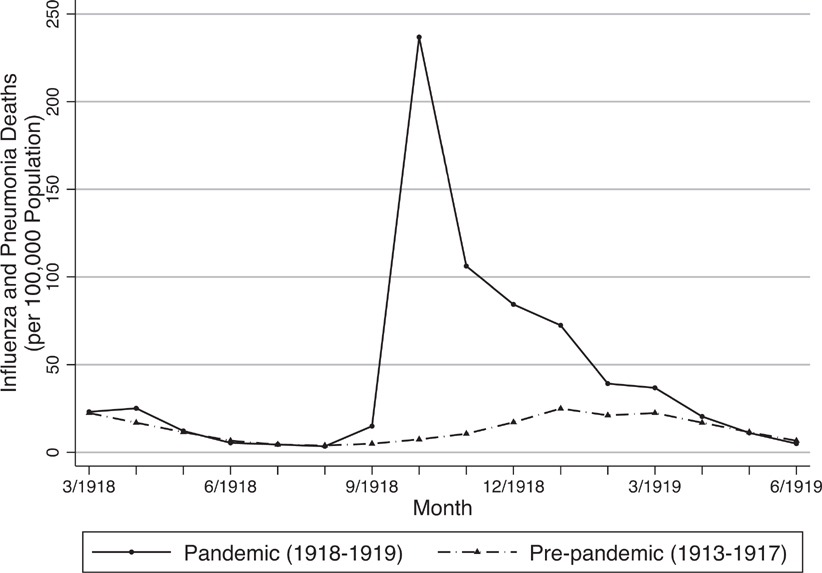
Figure 1 Influenza and Pneumonia Death Rates, March 1918–June 1919
The pandemic was caused by the H1N1 virus. Unlike the seasonal flu, which is typically caused by slight variations in pre-existing strains, the vast majority of individuals lacked immunity to the virus.Footnote 1 Approximately 30 percent of the U.S. population contracted the H1N1 virus in 1918–1919, and fatality rates among those who contracted the virus exceeded 2.5 percent, which is far higher than the typical mortality of 0.1 percent (Collins Reference Collins1930). The Spanish Flu was also characterized by an unusual “W” age distribution of mortality (see Online Appendix Figure A.1). The high mortality rates among young adults have been linked to an overreaction of the immune system (Barry Reference Barry2004). Infant mortality was caused by both postnatal exposure to the virus and higher rates of premature birth (Reid Reference Reid2005).
The pandemic first appeared in the United States as part of a mild influenza outbreak during the spring of 1918. Historians have sought to identify the site of origin of the 1918 Influenza Pandemic. Some accounts suggest that the first human infection occurred in Haskell County, Kansas between late January and early February 1918, and then spread to Europe by U.S. troops (Barry Reference Barry2004). It is believed that a mutation in the strain during the summer led to a sharp increase in virulence.
The most serious wave of the pandemic originated in Camp Devens near Boston in the first week of September 1918, and then spread rapidly throughout the country. By mid-September, the pandemic had surfaced in most East Coast cities and then moved westward, diffusing nationwide by early October (Sydenstricker Reference Sydenstricker1918).
Determinants of Pandemic Mortality
There were wide cross-city differences in pandemic severity. Pandemic mortality was more than 2.5 times higher in cities at the 90th percentile relative to cities at the 10th percentile.Footnote 2 Differences in pandemic mortality were large even among cities within the same state. For example, mortality rates in Gary, Indiana, were more than twice as high as those in Indianapolis. Although researchers have commented on the differences, there is little consensus on the underlying causes (Huntington Reference Huntington1923; Crosby Reference Crosby1989; Kolata Reference Kolata1999; Brainerd and Siegler Reference Brainerd and Siegler2003).
The medical and public health response to the pandemic appears to have been largely ineffective. Antibiotics had not yet been developed, and so could not be used to treat the bacterial pneumonia that often developed, and medicine, more generally, had little to offer beyond palliative care. Municipalities were often slow to adopt preventative measures, which included bans of public gatherings, regulations against spitting in public, and campaigns to the wearing of masks. Most researchers consider these public interventions to have had little effect on pandemic mortality (Brainerd and Siegler Reference Brainerd and Siegler2003; Crosby Reference Crosby1989).Footnote 3
Historians have argued that the timing of local onset, driven in part by the movement of military personnel, influenced pandemic mortality (Barry Reference Barry2004; Byerly Reference Byerly2010; Sydenstricker Reference Sydenstricker1918; Crosby Reference Crosby1989). Some accounts suggest that the virus weakened substantially in mid-October of 1918, and that cities that experienced later outbreak were exposed to a less virulent strain. Poverty has also been linked to pandemic mortality, both because of higher transmission in poor neighborhoods and lower levels of baseline health capital, although notably no relationship has been found between crowding, measured by population density, and pandemic mortality (Clay, Lewis, and Severnini Reference Clay, Lewis and Severnini2018; Grantz et al. Reference Grantz, Rane, Salje and Glass2016; Tuckel et al. Reference Tuckel, Sassler, Maisel and Leykam2006).
Pandemic Severity, Air Pollution, and Coal-Fired Electricity Generation
Air pollution has received almost no attention from the historical literature on the pandemic, despite emerging evidence that air pollution exacerbates pandemics. In randomized control trials, mice exposed to higher levels of particulate matter (PM) experienced increased mortality when infected with a common strain of the influenza virus (Hahon et al. Reference Hahon, Booth, Green and Lewis1985; Harrod et al. Reference Harrod, Jaramillo, Rosenberger and Wang2003; Lee et al. Reference Lee, Saravia, You and Shrestha2014). Microbiology studies of respiratory cells also identify a link between pollution exposure and respiratory infection. Respiratory cells are the primary site for influenza virus infection and replication, and PM exposure increases the viral-load post-infection (Jaspers et al. Reference Jaspers, Ciencewicki, Zhang and Brighton2005). Air pollution has also been shown to increase the severity of bacterial infections in the lungs (Jakab Reference Jakab1993).
The effects of air pollution may have been particularly acute during the 1918 pandemic given the pathology of the H1N1 virus. Pandemic mortality was often caused by a secondary infection, such as bacterial pneumonia. Contemporary researchers noted the impact of the pandemic virus on lungs. As reported in the Journal of the American Medical Association, doctors noted that “lung lesions, complex and variable, struck one as being quite different in character to anything one had met with at all commonly in thousands of autopsies one had performed during the last 20 years” (Ireland Reference Ireland1928, p. 150).
Although systematic cross-city information on air quality was not available until the mid-1950s, intermittent monitor readings during the early twentieth century suggest that air pollution was severe and widely varied across cities. Average levels of total suspended particulates (TSP) air pollution across 15 large U.S. cities were seven times higher than the annual threshold and twice the maximum daily threshold initially set under the Clean Air Act Amendments of 1970 (Online Appendix Table A.2). In 1912, the Bureau of Mines reported that 23 of 28 cities with populations with more than 200,000 were trying to combat smoke (Online Appendix Table A.1). Dozens of smaller cities also passed ordinances.
Electricity generation was a significant contributor to urban air pollution. In 1912, electricity generating plants accounted for 44 percent of visible smoke in Chicago, while residential coal consumption contributed just 4 percent (Goss Reference Goss1915).Footnote 4 Moreover, coal-fired power plants operated continuously throughout the fall of 1918, whereas residential coal consumption was concentrated in the winter months (Barreca, Clay, and Tarr Reference Barreca, Clay and Tarr2016).
There were large differences in the sources of electricity generation based on local availability of inputs. For example, both Grand Rapids and Lansing, Michigan had similar installed electricity capacity in 1915, although Grand Rapids, which had more abundant sources of hydro potential, generated more than twice as much power from hydroelectricity. At the state level, there is a positive relationship between total coal consumption and coal-fired generating capacity, and a negative relationship between total coal consumption and hydro capacity (Online Appendix Figure A.2), reflecting the fact that coal-fired power was concentrated in the midwestern states with abundant coal resources.
Data Construction and City Characteristics by Coal-Fired Capacity
To study the impact of air pollution on pandemic severity, we combine information on city coal-fired capacity with a panel dataset on mortality.Footnote 5 Infant and all-age deaths were collected from the Mortality Statistics for a panel of 180 registration cities for the period 1915–1925.Footnote 6 We begin with an initial sample of 283 cities with a population of at least 20,000 in 1921. From this sample, we drop 88 cities with missing information on covariates, and exclude an additional 15 cities located in states that did not use coal for electricity generation, leaving a final sample of 180 cities. Cities are linked to pre-pandemic county-level demographic and economic characteristics drawn from the census of population and census of manufacturing (Haines and ICPSR Reference Haines2010).
We combine the data on infant and all-age deaths with information on city population and births in 1921 to calculate the infant mortality rates per 1,000 live births in 1921, and the all-age mortality rates per 10,000 city residents in 1921. Infant mortality is widely used in studies of air pollution, since infants are especially vulnerable to environmental exposure and current air pollution concentrations are a better reflection of lifetime exposure (Currie et al. Reference Currie, Graff-Zivin, Mullen and Neidell2014). Contemporary evidence suggests that both infant and all-age deaths were accurately recorded, although there was substantial underregistration of births, particularly among minority populations (Grove Reference Grove1943). Because underreporting of births may bias estimates in panel regression analyses (Eriksson, Niemesh, and Thomasson Reference Eriksson, Niemesh and Thomasson2017), we explore the sensitivity of the main results to several alternative measures of the infant mortality rate.
To construct a proxy for city-level pollution, we digitized information from a 1915 federal report on the location and capacity of coal-fired and hydroelectric power stations with installed capacity of at least five megawatts (U.S. Department of Agriculture 1916). These data account for 67 percent of installed coal-fired capacity and 83 percent of installed hydroelectric capacity in 1915.Footnote 7 We calculate total coal-fired capacity within a 30-mile radius of each city-centroid, and classify cities into terciles (low, medium, high) of coal-fired capacity. This radius was chosen to capture the fact that the majority of power plant emissions are dispersed locally (Seinfeld and Pandis Reference Seinfeld and Pandis2012).Footnote 8 To assess whether local coal-fired capacity was related to urban air pollution, we estimate city-level regressions that compare the relationship between coal-fired capacity in 1915 and TSP concentrations in the mid-twentieth century, controlling for city population, the urban share, and total manufacturing employment.Footnote 9 Despite a lag of almost 50 years, there is a clear positive relationship between coal-fired capacity and measured air pollution, and a negative relationship between hydro capacity and TSP concentrations (Online Appendix Figure A.3).
Coal-fired generating capacity widely varied across cities. Cities with more coal capacity tended to have larger manufacturing sectors, perhaps reflecting higher electricity demand. They also tended to use more coal for residential purposes, reflecting greater local availability (see Online Appendix Table A.3). Despite these differences, almost half of the cross-city variation in coal capacity cannot be explained by standard socioeconomic measures. This idiosyncratic variation in coal capacity across cities will form the basis of our empirical strategy.
Table 1 (column 1) reports mean characteristics for the sample of 180 cities. The infant mortality rate was 86 per 1,000 live births, and decreased over the sample period (Figure 2a). The all-age mortality rate was 138 per 10,000 residents, and remained roughly stable in non-pandemic years (Figure 2b). During the pandemic year, infant mortality exceeded its trend by 19 percent and all-age mortality exceeded its trend by 35 percent.
Table 1 Summary Statistics

* = Significant at the 10 percent level.
** = Significant at the 5 percent level.
*** = Significant at the 1 percent level.
Notes: Column 1 reports unweighted average values for the 180 sample cities. Columns 2 and 3 report the difference in each relevant characteristic for medium and high coal cities relative to low coal cities. These estimated differences are obtained from a single regression of the indicated characteristics on a dummy for medium and high coal (low coal is the omitted category) conditional on city longitude and latitude. Columns 4 and 5 report the estimated difference in each characteristic conditional on longitude and latitude and a city-specific propensity score. The propensity score is obtained from an order probit regression model of tercile of coal capacity on baseline city socioeconomic conditions (log population, fraction white, fraction foreign born, fraction urban, log manufacturing employment, log manufacturing payroll per worker, and tercile of residential coal consumption). Robust standard errors are reported in parentheses.
Sources: Authors’ calculations based on the Mortality Statistics, Haines and ICPSR (Reference Haines2010), and the U.S. Department of Agriculture (1916) (see text for details).

Figure 2 Infant and All-Age Mortality, 1915–1925
Table 1 reports estimated differences in city characteristics for medium coal capacity and high coal capacity relative to low coal capacity cities. We report unadjusted differences in outcomes (cols. 2 and 3) and propensity score adjusted differences (cols. 4 and 5).Footnote 10 Over the full period, there is no statistically significant difference in unadjusted or adjusted infant mortality rates by coal capacity. There is a slightly negative relationship between all-age mortality and coal capacity, indicating that healthier workers were somewhat more likely to reside in highly polluted cities, potentially drawn to better labor market opportunities. These differences are eliminated after adjusting for baseline socioeconomic conditions in columns 4 and 5.Footnote 11 High and low coal cities are estimated to have had similar trends in mortality both prior to the pandemic and over the entire sample period. Despite these similarities in non-pandemic years, high coal cities experienced a differential rise in mortality in 1918. Cities in the top tercile had excess infant mortality rates that were 10.8 percentage points higher than cities in the bottom tercile, and the gap in excess all-age mortality rates was 6.3 percentage points. We also estimate large differences in coal-fired capacity across the three terciles that are not explained by baseline socioeconomic conditions (Panel B).
There were other differences in socioeconomic characteristics across the three terciles of coal-fired capacity. High coal cities were more populous, had larger manufacturing sectors, had a higher concentration of foreign-born residents, and burned more coal for residential use (Panels C and D). Adjusting for the propensity score largely eliminates these differences. To the extent that high and low coal cities were different in either pre-trends or levels, our empirical controls for both city and year fixed effects, and allows for differential non-pandemic trends in mortality and differential changes in mortality in 1918 according to each observable pre-pandemic characteristic and baseline dependent variables.
Empirical Framework
To study the effects of air pollution on pandemic mortality, we adopt a difference-in-differences approach that combines the sharp timing of the pandemic with large cross-city differences in coal-fired capacity. The empirical analysis is based on a comparison of average changes in mortality during the pandemic across cities with higher levels of coal-fired capacity relative to changes in mortality in cities with lower levels of coal-fired capacity that had similar pre-pandemic observable characteristics and similar pre-pandemic mortality rates.Footnote 12 Formally, outcome Yct in city c and year t is regressed on city and year fixed effects (μc and λt ), indicators for high coal capacity (Hc ) and medium coal capacity (Mc ) that are each interacted with year fixed effects, separate controls for pre-pandemic mortality in 1915 and 1916 (Yc,pre) that are each interacted with year fixed effects, pre-pandemic county characteristics (Xc ) that are each interacted with a linear time trend and an indicator for 1918, and an error term (εct ): ${Y_{ct}} = {\beta _{1t}}{H_c} \cdot {\lambda _t} + {\beta _{2t}}{M_c} \cdot {\lambda _t} + {\gamma _t}{Y_{c,pre}} \cdot {\lambda _t} + \theta {X_c} \cdot t + {\theta _{18}}{X_c} \cdot I(18) + {\mu _c} + {\lambda _t} + {\varepsilon _{ct}}.$
The coefficients for coal capacity (β 1t and β 2t ) are allowed to vary in each year. We set 1917 as the reference year. As a result, each coefficient β 1t (β 2t ) captures the differential change in mortality from 1917 to year t in high (medium) coal cities relative to the change in mortality in low coal cities over the same period.
Equation (1) includes controls for baseline mortality in 1915 and 1916 (separately) interacted with year fixed effects. These controls allow for differences in pandemic severity according to baseline population health. The vector Xc includes the baseline demographic and economic control reported in Table 1, panel C, along with city longitude and latitude. Each variable is interacted with a linear time trend and a dummy variable for 1918.Footnote 13 These controls allow for both differential trends in mortality and differential changes in mortality during the pandemic year according to city socioeconomic conditions and geography.
The identification assumption is that the increase in mortality in 1918 would have been similar across the three groups of cities in the absence of coal capacity differences. In practice, this assumption must hold after allowing for differential changes in mortality related to baseline city characteristics and pre-pandemic mortality rates. In the next section we demonstrate the validity of the empirical methodology and assess threats to identification.
Two other estimation details are worth noting. First, the regressions are unweighted. Standard errors are clustered at the city level to adjust for heteroskedasticity and within-city correlation over time.
Results
Infant and All-Age Mortality
To illustrate the empirical approach, Figure 3 graphs estimated βs with different sets of controls (see equation (1)).Footnote 14 This “event-study” design compares changes in mortality in each year from 1915 to 1925 relative to the 1917 baseline year. The figure allows us to assess the identification assumption that absent the pandemic, mortality in high and low coal cities would have trended similarly in 1918. The left-hand figures report the coefficient estimates from regression models that include city fixed effects, year fixed effects, and geographic controls that capture the spread of the virus.Footnote 15 The right-hand figures report the coefficient estimates from the fully specified regression model reported in equation (1), with additional controls for 1915 and 1916 mortality interacted with year along with the full set of demographic and economic covariates. Panel A reports the results for infant mortality, and panel B for all-age mortality.

Figure 3 Estimated Differences in Mortality by Coal-Fired Capacity, 1915–1925
In 1918, infant mortality and all-age mortality in high-capacity and medium-capacity cities increased relative to low-capacity cities. The rise in 1918 mortality was particularly large in high-capacity cities. The relative increases in mortality were temporary, and in the years following the pandemic, mortality changes were similar across the three groups of cities. In contrast, there is no statistically significant relationship between coal capacity and changes in mortality in non-pandemic years, supporting our identifying assumption that mortality would have trended similarly in 1918 in the absence of the pandemic.
Table 2, columns 1–3, reports results for infant mortality from estimating equation (1). In column 1, we include city and year fixed effects along with controls for baseline mortality and geography. In column 2, we add controls for baseline city demographic characteristics, and, in column 3, we include the full set of economic controls as described in equation (1). There is a strong relationship between coal capacity and pandemic-related infant mortality that is stable across the different specifications. In 1918, infant mortality increased by 11.0 percent more in high-capacity cities and 7.8 percent more in medium-capacity cities than in low-capacity cities (column 3).
Table 2 The Effect of the Pandemic on Mortality, by Coal-Fired Capacity

* = Significant at the 10 percent level.
** = Significant at the 5 percent level.
*** = Significant at the 1 percent level.
Notes: Each column reports the coefficient estimates from a different regression from versions of equation (1) in the text. The coefficient estimates represent the interaction effects for medium vs. low coal (β 2,1918) and high vs. low coal (β 1,1918). Geographic controls include city longitude and latitude. Demographic controls include city population, and county-level controls for fraction urban, fraction foreign born, and fraction nonwhite. Economic controls include manufacturing employment, manufacturing payroll per worker, and tercile of residential coal use. Controls are interacted with a linear time and an indicator for 1918. Standard errors are clustered at the city-level.
Sources: See Table 1.
There were similarly large relative increases in pandemic all-age mortality in high coal cities. Table 2, columns 4–6, reports the coefficient estimates for the 1918 interaction effect for high and medium coal cities. In 1918, all-age mortality increased by an additional 9.6 percent in high-capacity cities and 5.4 percent in medium-capacity cities as compared to changes in low-capacity cities (column 6).
The differential increases in mortality in high- and medium-capacity cities during the pandemic year are consistent with the epidemiological and experimental evidence on the role of air pollution in increasing influenza morbidity and mortality. The observed relationships could reflect the effects of air pollution exposure in the months prior to the pandemic, exposure during the pandemic, or some combination of the two.
Because the regression models control flexibly for trends based on pre-pandemic mortality rates, the coefficient estimates capture the impact of coal capacity on pandemic mortality across cities with similar baseline health. In the fully specified model, we also include baseline demographic and economic covariates, each interacted with a time trend and a 1918 dummy to allow for differences in pandemic mortality according to each pre-pandemic factor. The fact that these covariates have very little impact on the main coefficient estimates strongly suggests that there was an independent relationship between coal capacity and pandemic mortality that was not driven by differences in population characteristics or industrial composition.
To quantify the impact of air pollution on pandemic severity we calculate the number of deaths attributable to coal, based on the coefficient estimates from Table 2 and compare these to the total number of excess deaths in 1918 in the sample population. Table 3 reports the results. The top panel reports the estimates of the total number of excess deaths in 1918 for cities in each of the three terciles of coal capacity (see Online Appendix B). In total, we calculate that there were 158,000 excess deaths in 1918 in the sample.Footnote 16 Given that our sample comprises roughly 30 percent of the U.S. population, these calculations fall within the range of previous estimates of total U.S. pandemic mortality (Crosby Reference Crosby1989).
Table 3 Pandemic-Related Deaths Averted by Reducing Coal-Fired Capacity

Notes: Excess deaths in 1918 are calculated as the difference between observed mortality in 1918 and predicted mortality in 1918 based on a linear city-specific trend for the period 1915 to 1925. Estimates for approach 1 are calculated by multiplying the total population by the change in mortality probability implied by the estimated coefficients from Table 2, column 6. Estimates for approach 2 are calculated by subtracting the coefficient estimates from Table 2, column 6 from observed excess mortality in 1918 and multiplying by total population. See Online Appendix B for details of calculations.
Sources: See Table 1.
We evaluate the number of pandemic-related deaths in a counterfactual scenario in which coal capacity in high and medium is reduced to the low-capacity level. The calculations are derived based on the coefficient estimates in column 6 of Table 2. We rely on two different approaches to calculate the number of deaths averted. In the first approach, we multiply the total exposed population by the change in mortality probability implied by the regression coefficients. In the second approach, we compare the observed excess 1918 mortality rate to the counterfactual excess mortality rate implied by the regression estimates (see Online Appendix B for calculations). Both approaches yield large counterfactual reductions in mortality. We calculate that 30,000 to 42,000 total deaths (5,600 to 6,500 infant deaths) would have been averted, a 19 to 26 percent reduction in pandemic mortality. The majority of the deaths averted would have occurred in high-capacity cities. These cities tended to be more populous, so the health impacts of coal were particularly severe.
The economic costs of air pollution during the pandemic were substantial. Applying a $1.1 million (2015 dollars) value of a statistical life in 1920 (Costa and Kahn Reference Costa and Kahn2004), we calculate that excess mortality in high and medium coal cities led to a loss of $45.9 billion, equivalent to almost 6 percent of total U.S. GDP in 1918. These losses do not account for the morbidity effects and the losses in worker output in 1918.
Poverty, Timing of Onset, Local Interventions, and Pandemic Mortality
Having established a link between coal capacity and pandemic mortality, we now explore other potential determinants of pandemic severity. Table 4 explores the importance of factors related to city poverty and the geographic spread of the pandemic throughout the country.
Table 4 Other Determinants of Pandemic Severity

* = Significant at the 10 percent level.
** = Significant at the 5 percent level.
*** = Significant at the 1 percent level.
Notes: Each column reports the coefficient estimates from a different regression. All models include the full set of controls reported in Table 2, column 3, excluding 1915 and 1916 mortality × year in columns 1, 2, 5, 6, 7, 10, and excluding geographic controls in columns 3, 4, 5, 8, 9, 10. The coefficient estimates represent the interaction effects for medium vs. low coal (β 2,1918), high vs. low coal (β 1,1918), and other determinants of pandemic mortality. Baseline typhoid mortality is calculated as the average typhoid mortality rate between 1900 and 1905. Late pandemic arrival is a dummy variable equal to one for cities whose initial recorded onset of the pandemic occurred after September 27, 1918. Near WWI military base is a dummy variable equal to one for cities that were below median distance from a WWI army training camp. Standard errors are clustered at the city-level.
Sources: Typhoid mortality is from Whippel (Reference Almond1908); the timing of pandemic onset is from Sydenstricker (Reference Sydenstricker1918); the location of WWI army training camps is from the U.S. War Department (1919); other sources are described in Table 1.
We assess the impact of various proxies for city poverty on pandemic-related mortality. We include measures of the percent white, percent foreign born, and the typhoid rate in 1900–1905, an indicator for poor quality of drinking water (Beach et al. Reference Beach, Ferrie, Saavedra and Troesken2016), all interacted with an indicator for 1918.Footnote 17 To separately identify the role of these poverty proxies, these regression models do not include baseline mortality controls. The coefficient estimates reflect the extent to which differences in various measures of socioeconomic conditions were related to pandemic severity.
We find some evidence that city poverty and baseline health conditions were related to pandemic mortality (Table 4, columns 1 and 2). Higher concentrations of foreign born are associated with excess all-age mortality, and the fraction white is negatively related to pandemic mortality although the coefficient estimates are not statistically significant. Poor water quality, as proxied by typhoid mortality, is also positively related to all-age pandemic mortality.
Historians have argued that the timing of pandemic onset was related to its severity (Crosby Reference Crosby1989; Sydenstricker Reference Sydenstricker1918). Researchers have claimed that the virus weakened over the course of the fall of 1918, so that locations that experienced a delayed onset were exposed to a less virulent strain. The ability of public officials to respond to the outbreak may also have been related to the timing of local onset.
We assess whether factors related to the timing of onset were related to pandemic mortality. For this analysis, we omit controls for longitude and latitude to separately identify the role of geography. First, we use information on the week of pandemic onset from Edgar Sydenstricker (Reference Sydenstricker1918). The pandemic first surfaced along the East Coast in early September, and moved westward, diffusing nationwide by mid-October. We construct a dummy variable for “late” arrival cities that experienced onset after September 27, and interact this variable with an indicator for 1918 to allow for differences in severity based on the time of onset.Footnote 18 The results (reported in column 3) show that both infant and all-age mortality were significantly lower in late arrival cities, consistent with previous claims about the evolution of the virus.
Next, we assess the role of WWI in influencing local pandemic severity. The movement of military personnel is believed to have been an important determinant of pandemic timing. Alfred Crosby (Reference Crosby1989), Gina Kolata (Reference Almond2001), John Barry (Reference Barry2004), and Carol Byerly (Reference Byerly2010) provide detailed accounts of the pandemic in the military and the role of the Navy and Army in its spread. We digitized information on the location of major army training camps in 1918 (U.S. War Department 1919, p. 1519), and construct a dummy variable for whether a city was below- or above-median distance from a base. We interact this variable with a 1918 indicator to allow for differences in pandemic severity according to exposure to WWI military bases. The results (column 4) show that infant mortality was significantly higher in cities near a base. The coefficient estimates for all-age mortality are also positive, albeit smaller in magnitude and statistically insignificant.
Overall, the results in Table 4 support the historical narrative that both urban poverty and factors related to the timing of pandemic onset were related to local severity. Importantly, across all these alternative specifications and different samples, the impact of coal capacity remains stable, suggesting that the main results were not driven by one of these alternative mechanisms.
Some researchers have argued that other local public interventions, such as quarantines and bans on public gatherings, influenced severity (Markel et al. Reference Markel, Lipman, Navarro and Sloan2007). To assess the role of the local public health effort, we use data from Markel et al. (Reference Markel, Lipman, Navarro and Sloan2007) on local interventions for a subsample of 32 cities and construct indicators for early and long-term interventions following their classification. We interact these indicators with the 1918 dummy, and re-estimate a simplified version of equation (1) for the sub-sample of cities.Footnote 19
The results are reported in Table 5. For comparison, we report the estimates from this modified specification in column 1. Restricting the sample to the 32 quarantine cities, the coefficient estimates for medium capacity are not statistically significant, although the coefficients for high coal-fired capacity remain statistically significant and similar in magnitude to the estimates in Table 2. The coefficient estimates for early and long-term intervention are negative although not statistically significant. Broadly, these findings support the conclusions of Markel et al. (Reference Markel, Lipman, Navarro and Sloan2007) and Bootsma and Ferguson (Reference Bootsma and Ferguson2007) that local public health initiatives may have played a role in mitigating the effects of the pandemic.
Table 5 Local Interventions and Pandemic Severity

* = Significant at the 10 percent level.
** = Significant at the 5 percent level.
*** = Significant at the 1 percent level.
Notes: Each column reports the coefficient estimates from a different regression. All models are estimated for a restricted set of controls that include city and year fixed effects, and longitude/latitude and city population (each variable interacted with a linear time trend and an indicator for 1918). The coefficient estimates represent the interaction effects for medium vs. low coal (β 2,1918), high vs. low coal (β 1,1918), and characteristics of local nonpharmaceutical interventions for a sample of 32 cities from Market et al. (Reference Almond2007). Early and long interventions are classified according to Market et al. (Reference Almond2007), where “early intervention” is a dummy variable for cities that implemented nonpharmaceutical interventions within one week of pandemic onset, and “long intervention” is a dummy variable for cities that maintained nonpharmaceutical interventions for at least 65 days. Standard errors are clustered at the city-level.
Sources: Data on nonpharmaceutical interventions are from Market et al. (Reference Almond2007); other sources are described in Table 1.
Robustness Checks
One potential concern with the previous results is misreporting of the mortality rate. Although infant and all-age deaths are generally thought to have been accurately recorded, underregistration of births could bias the estimates for infant mortality (Eriksson, Niemesh and Thomasson Reference Eriksson, Niemesh and Thomasson2017). Moreover, because our measure of the infant mortality rate is constructed based on births in 1921 rather than contemporaneous births, annual fluctuations in fertility could bias the main estimates. We explore the sensitivity of the results to two alternate measures of the infant mortality rate: infant deaths per 1,000 annual births and infant deaths per 10,000 city residents in 1921. Estimates based on the first measure will not be biased by annual fluctuations in fertility, although because a number of cities began collecting information on births midway through the sample period, we must omit roughly one-quarter of the sample. Meanwhile, the second measure will not be affected by reporting error due to the under-registration of births.
Table 6 reports the results based on the alternate measures of infant mortality, which are both highly correlated with the original dependent variable. For reference, column 1 reports the baseline results. Column 2 reports the results based on infant deaths per 1,000 annual births. Despite the limited sample size, the estimated effects are similar in magnitude to the original findings. Column 3 reports the results based on infant death per city population in 1921. The coefficient estimates are also very similar to the baseline estimates, providing confidence that the main findings were not influenced by mismeasurement of births.
Table 6 Robustness Tests: Alternative Measures of Infant Mortality

* = Significant at the 10 percent level.
** = Significant at the 5 percent level.
*** = Significant at the 1 percent level.
Notes: Each column reports the coefficient estimates from a different regression. All models include the full set of controls reported in Table 2, column 3. The coefficient estimates represent the interaction effects for medium vs. low coal (β 2,1918) and high vs. low coal (β 1,1918). Standard errors are clustered at the city-level.
Sources: See Table 1.
Table 7 provides a number of robustness checks. For reference, column 1 reports the baseline specification. Columns (2) to (4) explore sensitivity to alternate control variables. In column 2, we add controls for linear state-specific trends to allow for differential trends in mortality across states. The results are not affected by these covariates. In column 3, we replace the control for log population with log population density. This covariate allows for differences in pandemic transmission, for example, due to crowding. Because we lack information on contemporaneous population density, this variable is constructed by dividing city population in 1921 by city area reported in the 1944 City Books (Haines and ICPSR Reference Haines2010).Footnote 20 The coefficient estimates are very similar to the main findings, consistent with epidemiological evidence showing no association between population density and pandemic mortality (Grantz et al. Reference Grantz, Rane, Salje and Glass2016). In column (4), we explore the sensitivity of the main findings to controls for the population age structure. We add controls for the fraction of the population age 18 to 44, who were particularly susceptible to the virus. The main findings are unaffected by this covariate.
Table 7 Robustness Tests

* = significance at the 10 percent level.
** = significance at the 5 percent level.
*** = significance at the 1 percent level.
Notes: Each column reports the coefficient estimates from a different regression. All models include the full set of controls reported in Table 2, column 3.
Standard errors are clustered at the city-level.
Columns (5) to (8) examine the sensitivity of the results to alternate specifications and samples. In column 5, we re-estimate the model based on the mortality rate in levels rather than logs. The estimated effects are statistically significant and economically important. For infant mortality, the coefficient estimates imply increases in pandemic mortality of 15 (=13.0/85.5) percent and 9 (=7.6/85.5) percent in high coal and medium coal cities relative to low coal cities. For all-age mortality, the implied relative increases are 8 (=11.0/138.2) percent and 15 (=21.1/138.2) percent in high and medium coal cities. In column 6, we report the results, dropping cities for which more than one year of mortality data is missing. In column 7, we drop cities in the South. The coefficients on coal-fired capacity remain similar to the baseline values in sign, significance, and magnitude. In column 8, we re-estimate the regressions for cities with at least 50,000 residents in 1921 to examine the sensitivity of the results to outlier mortality rates in smaller cities. The results are not sensitive to this sample restriction.Footnote 21
To conclude the empirical analysis, we provide two additional tests of the research design. First, we explore heterogeneity in the coal-pandemic relationship according to average city wind speed. Intuitively, the local impact of coal consumption should be mitigated by higher wind speeds, which disperse pollutants over a wider region (e.g., Wang and Ogawa Reference Wang and Ogawa2015). We assemble information on average annual speed at an elevation of 80 meters from the U.S. Department of Energy (2017), to identify cities above-median and below-median wind, and allow the effects of coal capacity to vary according to this variable.Footnote 22 The results show uniformly larger mortality effects in low wind cities (column 9), consistent with higher winds having mitigating the local health impacts of air pollution during the pandemic.
Second, we estimate a set of placebo regressions based on hydroelectric capacity, which generated electricity but was emissions free. In these regressions we interact indicators for medium and high hydroelectric capacity with 1918. The results show no significant relationship between hydro capacity and excess infant or all-age mortality in 1918 (column 10).Footnote 23
Concluding Remarks
The 1918 Influenza Pandemic was an exceptional historical episode, with death rates 5 to 20 times higher than typical pandemics. A century later, the “Spanish Flu” continues to be an active area of historical analysis, with researchers seeking to understand its origin, the sources of its virulence, and its epidemiological features. Despite ongoing research, basic questions remain about the spread of the virus, and the sources of the stark regional patterns in mortality.
This article provides new evidence on the role of air pollution in exacerbating the pandemic. The effects of air pollution on pandemic mortality were sizeable. Cities with high levels of coal capacity collectively experienced tens of thousands of excess deaths in 1918. Our analysis suggests that pre-pandemic socioeconomic and health conditions also contributed to pandemic severity as did the timing of its spread throughout the country.
Despite improvements in preventative practices and the development of modern antiviral drugs and vaccines, a moderately severe modern pandemic could lead to 2 million excess deaths worldwide (Fan, Jamison, and Summers Reference Fan, Jamison and Summers2016), and a pandemic virus with similar pathogenicity to the 1918 virus would likely kill more than 100 million (Taubenberger and Morens Reference Taubenberger and Morens2006). A better understanding of the factors that influenced mortality during 1918 Influenza Pandemic may offer critical insights for the mitigation of contemporary pandemics.
Although air quality has improved dramatically over the past 100 years in the United States, urban air pollution remains a major problem in many developing countries. In fact, pollution in cities in India and China is comparable to levels in the United States in the early twentieth century (Online Appendix Table A.2). This study’s findings thus have particular relevance to the developing world, where air pollution is often severe and where there is limited medical infrastructure. Further research on more recent outbreaks may help shed light on the potential for improved medical treatments and targeted pollution abatement strategies to mitigate the risks posed by a global pandemic.


