


1. Introduction
Flow in porous media can be found in many natural and industrial applications, spanning different fields of science and engineering. Multiphase flows (Higdon Reference Higdon2013), gas transport (Ho & Webb Reference Ho and Webb2006), heat and mass transfer (Defraeye et al. Reference Defraeye, Blocken, Derome, Nicolai and Carmeliet2012), processes in batteries and energy harvesting devices (Pillai & Deenadayalan Reference Pillai and Deenadayalan2014), rivers flowing over sediment beds (Shen, Yuan & Phanikumar Reference Shen, Yuan and Phanikumar2020), petroleum reservoirs (Jansen Reference Jansen2011), aquifers (Medici et al. Reference Medici, Smeraglia, Torabi and Botter2021) and geological carbon sequestration (Abidoye, Khudaida & Das Reference Abidoye, Khudaida and Das2015), to name a few, all depend on properties of porous media flow. Porous media with relatively low permeabilities in which the flow occurs at low Reynolds numbers (Re) are prevalent in most applications. Porous media are also being explored as a means for passive control of external flows. In this regard, recent advances in manufacturing techniques are providing media with both high permeability, necessary for effective control, and high structural strength, essential for practical engineering applications (Guest & Szyniszewski Reference Guest and Szyniszewski2021). In such applications, the interstitial flow Reynolds numbers can reach values much higher than what has been explored so far, and certainly for values where the validity of the DF law may be in question.
The Darcy law relates the bulk pressure drop within a porous medium linearly to the bulk velocity and fluid viscosity and its validity is limited to low-Re flows since it captures only viscous effects. More generally, however, it requires corrections to accommodate for flows in media with a relatively high pore-scale Reynolds number, where the inertial effects can dominate over the viscous ones. Two famous extensions to the Darcy law are the Brinkman (Reference Brinkman1949) and the Forchheimer (Forchheimer Reference Forchheimer1901; Whitaker Reference Whitaker1996) corrections. The former attempts to include a viscous diffusive term in the momentum equation to capture large-scale diffusive effects (larger than the pore-scale motions), while the latter, of main interest in the present paper, aims to capture inertial effects by adding a nonlinear term to the Darcy law.
Prior work dealing with the use of porous media to control turbulent flow over surfaces include Rosti, Brandt & Pinelli (Reference Rosti, Brandt and Pinelli2018), who simulated turbulent channel flow over anisotropic porous substrates. The porous medium was represented using Darcy's law. They found a range of drag increase and reduction – influenced by the surface permeabilities in the wall parallel and normal directions. Samanta et al. (Reference Samanta, Vinuesa, Lashgari, Schlatter and Brandt2015) performed direct numerical simulation of a duct flow over a high porosity  $(\epsilon =0.95)$ medium, (the results of which were then experimentally examined by Suga, Okazaki & Kuwata Reference Suga, Okazaki and Kuwata2020), and observed a strong enhancement of secondary motions above the medium, and the appearance of spanwise rollers occurring in the simulations with the porous wall that were not observed in the smooth-wall simulations. These authors used a one-dimensional (1-D) Darcy–Forchheimer (DF) model for their porous-wall simulation. Gómez-de Segura & García-Mayoral (Reference Gómez-de Segura and García-Mayoral2019) used the two-dimensional (2-D) Darcy–Brinkman law to model anisotropic porous substrates for drag reduction applications. They found up to 25 % drag reduction, proportional to the difference between the streamwise and spanwise permeabilities, for small permeability substrates and low pore Reynolds number applications. They, however, reported drag increase for high permeability cases due to emergence of spanwise roller structures. This work was then complemented by the resolvent analysis of Chavarin et al. (Reference Chavarin, Gómez-de Segura, García-Mayoral and Luhar2021), leading almost to the same conclusions.
In general, passive control using porous materials is more effective with materials with high permeability, but this requirement often conflicts in engineering applications, with the need for high structural strength. However, in recent years, advances in materials, as well as fabrication/assembly of meta materials, is driving the emergence of porous materials that have high permeability as well as high structural strength, and this is opening new opportunities for passive flow control. For instance, Guest & Szyniszewski (Reference Guest and Szyniszewski2021, explained above) and Pelacci, Robins & Szyniszewski (Reference Pelacci, Robins and Szyniszewski2021) proposed three-dimensional (3-D) woven-lattice periodic structures with high permeability and high specific stiffness for turbulence control and drag reduction of flow over bluff bodies. The hydrodynamic drag was reduced by up to 45 % depending on the angular position of the porous insert on the cylinder substrate. Such high permeability materials allow interstitial flows with high Reynolds numbers, which are often far outside the range envisioned for the DF law.
The primary objectives of the current study are to examine the DF law for porous media flows with inclusion Reynolds numbers that range from  $O(1)$ to $O(1000)$ and to quantify the impact of phenomena such as vortex shedding and flow channelling on the flow characteristics and pressure loss through the material. Another objective is to modify the DF law to capture the effects of such nonlinear phenomena for different geometries at intermediate/high-Re regimes.
1.1. Darcy and Forchheimer laws
The dimensional DF law for stationary and spatially homogeneous flow, using the form employed by Joseph, Nield & Papanicolaou (Reference Joseph, Nield and Papanicolaou1982) and Wang, Thauvin & Mohanty (Reference Wang, Thauvin and Mohanty1999), reads
 \begin{equation} -\!\boldsymbol{\nabla}P_B={\mu}\boldsymbol{\mathsf{K}}_d^{{-}1} \boldsymbol{\cdot} \boldsymbol{U}_B + \rho \boldsymbol{\mathsf{F}}_d^{{-}1} \boldsymbol{\cdot} (U_B \boldsymbol{U}_B), \end{equation}
where  $\boldsymbol{\mathsf{K}}_d$ is the dimensional Darcy permeability tensor, $\boldsymbol{\mathsf{F}}_d$ is the dimensional Forchheimer correction tensor, $\boldsymbol {U}_B=({1}/{V_f})\int _{V_f}\boldsymbol {u} \,\text {d}V$ is the bulk velocity ( $V_f$ being the fluid-occupied domain, indicative of the medium's pore space, and $\boldsymbol {u}$ is the local velocity vector), $P_B=({1}/{V_f})\int _{V_f}p \,\text {d}V$ is the fluid bulk pressure ( $\kern 1.5pt p$ being the local pressure field), $\boldsymbol {\nabla }_i=\partial /\partial x_i$ is the gradient operator and $\rho$ and $\mu$ are the fluid density and dynamic viscosity (we consider cases without buoyancy). For unsteady situations, additional time averaging is included in the definitions of the bulk quantities. Note that $\boldsymbol{\mathsf{K}}_d$ and $\boldsymbol{\mathsf{F}}_d$ in (1.1) are defined in a manner that incorporates intrinsic averages for the velocity field. Throughout our study, the porosity of the porous media, denoted as $\epsilon$ and calculated as the ratio of fluid-occupied volume ( $V_f$) to the total domain volume ( $V_t$), is maintained as a constant value. However, it is worth noting that one could adjust the definitions of these tensors to include superficial averages (similar to the approach practiced by Whitaker Reference Whitaker1996) if necessary. By properly normalizing (1.1) with the magnitude of the bulk velocity, $U_B=(\boldsymbol {U}_B\boldsymbol {\cdot }\boldsymbol {U}_B)^{1/2}$, a length scale $a$ defined more precisely in § 2, $\rho$ and $\mu$, one obtains
 \begin{equation} -\boldsymbol{\nabla}P=\frac{1}{Re}\boldsymbol{\mathsf{K}}^{{-}1} \boldsymbol{\cdot} \boldsymbol{U}+\boldsymbol{\mathsf{F}}^{{-}1} \boldsymbol{\cdot} \boldsymbol{U}, \end{equation}
where  $\boldsymbol {U}=\boldsymbol {U}_B/U_B$, $P = P_B/(\rho U_B^2)$, $\boldsymbol{\mathsf{K}}=\boldsymbol{\mathsf{K}}_d/a^2$, $\boldsymbol{\mathsf{F}} = \boldsymbol{\mathsf{F}}_d/a$ are, respectively, the normalized velocity vector, the normalized pressure and the normalized Darcy and Forchheimer tensors. The length scale $a$ characterizes the size of inclusions in the porous medium. Also, the inclusion Reynolds number is $Re = \rho U_B a/ \mu$ and $\boldsymbol {\nabla }_i=a\partial /\partial x_i$ is the normalized gradient operator. There have been some attempts to relate $\boldsymbol{\mathsf{F}}$ to $\boldsymbol{\mathsf{K}}$ in past works (such as $\boldsymbol{\mathsf{F}}\propto \sqrt {\boldsymbol{\mathsf{K}}}$ in Ward Reference Ward1964; Knupp & Lage Reference Knupp and Lage1995), however, here, we consider a generic tensor for $\boldsymbol{\mathsf{F}}$, not necessarily dependent on $\boldsymbol{\mathsf{K}}$. We also recall that these tensors must be positive definite (in the sense that they have real positive eigen-values) as shown by Chen, Lyons & Qin (Reference Chen, Lyons and Qin2001), and that $\boldsymbol{\mathsf{K}}$ must be symmetric (Whitaker Reference Whitaker1996).
Many numerical investigations focusing on capturing the micro-structures of porous media, while uncovering intriguing flow characteristics in such media, have typically been conducted at relatively low Reynolds numbers (such as Kuwata & Suga Reference Kuwata and Suga2016; Kutscher, Geier & Krafczyk Reference Kutscher, Geier and Krafczyk2019; Kuwata, Tsuda & Suga Reference Kuwata, Tsuda and Suga2020). Computational costs of pore-resolving simulations increase rather rapidly with increasing Reynolds numbers. Hence there is strong interest in modelling the porous substrate via the DF law ((1.1) or its variants). The validity of the DF law for flows with inertial effects, porous medium anisotropy and dependence on the Reynolds number is still an ongoing subject of research even in light of the substantial prior work in this field (Edwards et al. Reference Edwards, Shapiro, Bar-Yoseph and Shapira1990; Agnaou, Lasseux & Ahmadi Reference Agnaou, Lasseux and Ahmadi2016, Reference Agnaou, Lasseux and Ahmadi2017; Rao, Kuznetsov & Jin Reference Rao, Kuznetsov and Jin2020; Wood, He & Apte Reference Wood, He and Apte2020). Given the growing interest of using high porosity (possibly high pore Reynolds numbers) anisotropic media for flow control, it is important to explore the validity of the DF law for such applications. Especially for intermediate and high pore-Re regimes, one expects the emergence of nonlinear phenomena such as vortex shedding, flow redirection effects and wake asymmetries, for which the validity of the DF law remains to be examined.
In this study, we examine the performance of the DF law for different random (typically isotropic) and arranged (typically more anisotropic) porous lattices, for a wide range of Reynolds numbers (from essentially Stokes flow to high pore-Re flows). To enable numerical simulations over a large range of parameters, we chose to restrict the cases studied to 2-D porous media geometries. We quantify the DF-law accuracy for different lattices and pore Reynolds number. Our aim is to use time-accurate pore-resolving simulation data to measure the permeability tensors and then to test whether application of the DF law with constant Forchheimer tensors in these same cases can reproduce the flow observed in the simulations. For cases in which results cannot be properly reproduced by a constant Forchheimer tensor, we illustrate some empirically motivated minimal extensions of the model, specifically taking into account flow orientation with respect to the geometric features of the porous media.
Section 2 describes the simulation set-ups and how the permeability tensors for the DF law are evaluated based on the simulated data. Results are provided in § 3, where we also compare the flow predicted by the DF law using the measured permeability tensors with the actual flow velocity. Some of the results show that the standard DF law requires modifications to account empirically for observed inertial effects. Section 4 provides experimental evidence for such effects. In § 5 a more general version of the DF law is proposed based on phenomenological observations. The model parameters are fitted to data and predictions are compared with data. Conclusions are presented in § 6.
2. Methodology
2.1. Simulation set-up
Figure 1 shows the five porous media used in this study. The computational domains cover  $32 a \times 32 a$, where $a$ is the inclusion length scale (i.e. square height for cases C1–4, and circle diameter for C5). Medium C1 consists of aligned square inclusions; medium C2, staggered square inclusions; medium C3, square inclusions with a low degree of randomness (only the inclusions’ position is chosen randomly); medium C4, square inclusions with high degree of randomness (where both position and orientation are chosen randomly); and medium C5, with randomly placed circular inclusions. All five media are designed to have a porosity of $\epsilon =V_f/V_t=0.75$ (since, in two dimensions, strictly speaking $\epsilon$ is the ratio of areas $\epsilon =A_f/A_t=0.75$). For all cases, the simulations sweep over 14 values of $Re=\{1, 5, 10, 20, 40, 60, 80, 100, 140, 180, 250, 400, 750, 1000\}$, capturing the fluid dynamics from Stokes-like behaviour at low $Re$, to highly nonlinear dynamics at high $Re$. The flow is driven by a pressure gradient with a prescribed angle $\alpha$ but whose magnitude is adjusted in each time step such that it yields a constant bulk velocity magnitude $U_B=1$ (irrespective of flow direction). The schematics describing $\alpha$ and $\beta$, the respective direction angles of $-\boldsymbol {\nabla }P$ and $\boldsymbol {U}$ with respect to the $x$-axis, are shown in figure 2.

Figure 1. Porous media geometries. The parameter  $a$ describes the inclusion length scale, i.e. square height for cases C1–4, and circle diameter for C5. For case C1, the spacings between elements are $a$ in both $x$ and $y$ directions. Case C2 is similar to case C1 but the inclusions being staggered every other column with height $a$ in the $y$ direction.

Figure 2. Schematics describing  $\alpha$ and $\beta$, the respective angles of $-\boldsymbol {\nabla }P$ and $\boldsymbol {U}$, in a 2-D configuration.
For each medium and at each  $Re$, the flow is simulated for 7 values of imposed pressure gradient angles $\alpha =\{0, 15, 30, 45, 60, 75, 90\}$ degrees. In total, $5\times 14\times 7=490$ simulations are performed, and to accommodate the computational costs of this large parameter sweep, we limit ourselves to 2-D time-accurate pore-resolving simulations using a sharp-interface Navier–Stokes immersed boundary solver (Mittal et al. Reference Mittal, Dong, Bozkurttas, Najjar, Vargas and Von Loebbecke2008). The solver uses a second-order finite difference for spatial discretization and a second-order Adams–Bashforth for time advancement, and has been widely employed and validated in previous studies (Seo & Mittal Reference Seo and Mittal2011; Aghaei-Jouybari et al. Reference Aghaei-Jouybari, Seo, Yuan, Mittal and Meneveau2022). The coordinates in the horizontal, vertical and normal (to the plane) directions are denoted by $x$,
$x$,  $y$ and $z$, respectively. The pressure is denoted by $p$ and the respective velocity components in $x$ and $y$ are denoted by $u$ and $v$. Periodic boundary conditions are applied in both the $x$ and $y$ directions for all the simulations, consistent with a spatially homogeneous medium and a domain that includes a large number of inclusions, as shown. The number of grid points in both $x$ and $y$ directions equals to $n_x=n_y=1280$, resulting in 40 grid points in each direction per inclusion length scale $a$.
$a$.
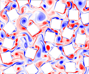
Figure 3 shows sample vorticity contours  $\omega _z$ for different media at low $Re=1$, intermediate $Re=100$ and high $Re=1000$, for two imposed pressure gradient angles ( $\alpha$) of $30$ and $60$ degrees. Note that the regions shown represent only a subset of the computational domains in each case (recall that the computational domain is $32 a$ on each side). We observed that the $Re=1$ flow is steady with no unsteady vortical motions, characteristic of Stokes flow. The onset of vortex shedding happens at intermediate Reynolds number, between 40 and 250 depending on the medium's geometry, which is manifested as meandering wakes in some of the cases at $Re=100$ in figure 3. For high $Re=1000$, strong vortex shedding occurs for all cases and the flows become spatially and temporally complex. The onset of this complexity for the intermediate and high Reynolds number flows is anticipated to impact the performance of the DF law. Therefore, the main objective of the present study is to test the DF-law performance, and to modify it in situations where its performance diminishes.

Figure 3. The normalized vorticity fields at low  $Re=1$, intermediate $Re=100$ and high $Re=1000$ for two $\alpha$ values of $30$ and $60$ degrees.
2.2. Measuring the Darcy and Forchheimer permeability tensors
In order to estimate the permeability tensors from our simulation results, we compute the mean velocity direction from the data in each case, and note the magnitude of the pressure gradient vector. We further enforce the condition of symmetry. As mentioned before, the Darcy tensor  $\boldsymbol{\mathsf{K}}$ has to be symmetric (Whitaker Reference Whitaker1996). While arguments have been made that $\boldsymbol{\mathsf{F}}$ could contain an antisymmetric part (Whitaker Reference Whitaker1996; Lasseux, Abbasian Arani & Ahmadi Reference Lasseux, Abbasian Arani and Ahmadi2011), it still has to remain positive definite (Chen et al. Reference Chen, Lyons and Qin2001). We here assume that $\boldsymbol{\mathsf{F}}$ is also symmetric to automatically ensure positive definiteness of $\boldsymbol{\mathsf{F}}$ and to minimize the number of elements to fit. This condition is enforced in the empirical determination of $\boldsymbol{\mathsf{K}}$ and $\boldsymbol{\mathsf{F}}$ as follows: we first predict the symmetric tensor $\boldsymbol{\mathsf{K}}$ in the low $Re$ Darcy regime. Equation (1.2) reduces to
 \begin{equation} \left.\begin{aligned}
\boldsymbol{U}&={-}Re
\boldsymbol{\mathsf{K}}\boldsymbol{\cdot}\boldsymbol{\nabla}P\\
\begin{bmatrix} U_1\\ U_2 \end{bmatrix}&={-}Re
\begin{bmatrix} {\mathsf{K}}_{11} & {\mathsf{K}}_{12}\\ {\mathsf{K}}_{12} & {\mathsf{K}}_{22}
\end{bmatrix} \begin{bmatrix} \partial_{1}P \\ \partial_2 P
\end{bmatrix}\\ &={-}\begin{bmatrix} Re \partial_{1} P & Re
\partial_2 P & 0 \\ 0 & Re \partial_{1} P & Re \partial_2 P
\end{bmatrix} \begin{bmatrix} {\mathsf{K}}_{11} \\ {\mathsf{K}}_{12}\\ {\mathsf{K}}_{22}
\end{bmatrix}, \end{aligned}\right\}
\end{equation}
\begin{equation} \left.\begin{aligned}
\boldsymbol{U}&={-}Re
\boldsymbol{\mathsf{K}}\boldsymbol{\cdot}\boldsymbol{\nabla}P\\
\begin{bmatrix} U_1\\ U_2 \end{bmatrix}&={-}Re
\begin{bmatrix} {\mathsf{K}}_{11} & {\mathsf{K}}_{12}\\ {\mathsf{K}}_{12} & {\mathsf{K}}_{22}
\end{bmatrix} \begin{bmatrix} \partial_{1}P \\ \partial_2 P
\end{bmatrix}\\ &={-}\begin{bmatrix} Re \partial_{1} P & Re
\partial_2 P & 0 \\ 0 & Re \partial_{1} P & Re \partial_2 P
\end{bmatrix} \begin{bmatrix} {\mathsf{K}}_{11} \\ {\mathsf{K}}_{12}\\ {\mathsf{K}}_{22}
\end{bmatrix}, \end{aligned}\right\}
\end{equation}
which holds for each data point. In the above equation,  $\partial _i P=\partial P/\partial x_i$ is the mean pressure gradient in each simulation. One can stack the right- and left-hand sides of the above equation for all data points as
 \begin{equation} \underbrace{\begin{bmatrix} \underbrace{\begin{bmatrix} U_1\\ U_2 \end{bmatrix}}_{point\ 1}\\ \underbrace{\begin{bmatrix} U_1\\ U_2 \end{bmatrix}}_{point\ 2}\\ \vdots\\ \underbrace{\begin{bmatrix} U_1\\ U_2 \end{bmatrix}}_{point\ n} \end{bmatrix}_{2n\times1}}_{\boldsymbol{V}} \boldsymbol{=}\underbrace{-\begin{bmatrix} \underbrace{\begin{bmatrix} Re \partial_{1}P & Re \partial_{2}P & 0 \\ 0 & Re \partial_{1}P & Re \partial_{2}P \end{bmatrix}}_{point\ 1}\\ \underbrace{\begin{bmatrix} Re \partial_{1}P & Re \partial_{2}P & 0 \\ 0 & Re \partial_{1}P & Re \partial_{2}P \end{bmatrix}}_{point\ 2}\\ \vdots\\ \underbrace{\begin{bmatrix} Re \partial_{1}P & Re \partial_{2}P & 0 \\ 0 & Re \partial_{1}P & Re \partial_{2}P \end{bmatrix}}_{point\ n} \end{bmatrix}_{2n\times3}}_{\boldsymbol{\mathsf{R}}} \underbrace{\begin{bmatrix} {\mathsf{K}}_{11} \\ {\mathsf{K}}_{12}\\ {\mathsf{K}}_{22} \end{bmatrix}_{3\times1}}_{\boldsymbol{K}_|}, \end{equation}
where  $n$ is the number of data points and $\boldsymbol {K}_|$ is the vertically stacked ( $3 \times 1)$ version of $\boldsymbol{\mathsf{K}}$. Equation (2.2) is an over-determined system of linear equations and the best estimate (in the least-square error sense) for $\boldsymbol {K}_|$ can be obtained via the pseudo-inverse $\boldsymbol{\mathsf{R}}$ (note the definition of $\boldsymbol{\mathsf{R}}$ includes the minus sign in (2.2)), i.e.
 \begin{equation} \boldsymbol{K}_{|{,best}}=(\boldsymbol{\mathsf{R}}^{\rm T} \boldsymbol{\mathsf{R}})^{{-}1}\boldsymbol{\mathsf{R}}^{\rm T} \boldsymbol{V}. \end{equation}
One can easily reconstruct the best estimate of tensor  $\boldsymbol{\mathsf{K}}$ from vector $\boldsymbol {K}_{|\textrm {,best}}$. The best estimate of tensor $\boldsymbol{\mathsf{F}}$ can be calculated similarly by substituting the best estimate of $\boldsymbol{\mathsf{K}}$ in (1.2) and reformulating the problem. It follows:
 \begin{equation} \left.\begin{gathered}
U\boldsymbol{U}={-}
\boldsymbol{\mathsf{F}}\boldsymbol{\cdot}
\boldsymbol{G}\\ \begin{bmatrix} UU_1\\ UU_2 \end{bmatrix}
={-} \begin{bmatrix} {\mathsf{F}}_{11} & {\mathsf{F}}_{12}\\ {\mathsf{F}}_{12} & {\mathsf{F}}_{22}
\end{bmatrix} \begin{bmatrix} G_1 \\ G_2 \end{bmatrix}\\
={-}\begin{bmatrix} G_1 & G_2 & 0 \\ 0 & G_1 & G_2
\end{bmatrix} \begin{bmatrix} {\mathsf{F}}_{11} \\ {\mathsf{F}}_{12}\\ {\mathsf{F}}_{22}
\end{bmatrix}, \end{gathered}\right\}
\end{equation}
\begin{equation} \left.\begin{gathered}
U\boldsymbol{U}={-}
\boldsymbol{\mathsf{F}}\boldsymbol{\cdot}
\boldsymbol{G}\\ \begin{bmatrix} UU_1\\ UU_2 \end{bmatrix}
={-} \begin{bmatrix} {\mathsf{F}}_{11} & {\mathsf{F}}_{12}\\ {\mathsf{F}}_{12} & {\mathsf{F}}_{22}
\end{bmatrix} \begin{bmatrix} G_1 \\ G_2 \end{bmatrix}\\
={-}\begin{bmatrix} G_1 & G_2 & 0 \\ 0 & G_1 & G_2
\end{bmatrix} \begin{bmatrix} {\mathsf{F}}_{11} \\ {\mathsf{F}}_{12}\\ {\mathsf{F}}_{22}
\end{bmatrix}, \end{gathered}\right\}
\end{equation}
where  $\boldsymbol {G} \equiv \boldsymbol {\nabla }P+({1}/{Re})\boldsymbol{\mathsf{K}}_{best}^{-1} \boldsymbol {\cdot } \boldsymbol {U}$. Note on the left-hand side $U=1$ for all simulations here. Again, stacking data of all points in (2.4) as follows:
 \begin{equation}
\underbrace{\begin{bmatrix} \underbrace{\begin{bmatrix}
UU_1\\ UU_2 \end{bmatrix}}_{point\ 1}\\
\underbrace{\begin{bmatrix} UU_1\\ UU_2
\end{bmatrix}}_{point\ 2}\\ \vdots\\
\underbrace{\begin{bmatrix} UU_1\\ UU_2
\end{bmatrix}}_{point\ n}
\end{bmatrix}_{2n\times1}}_{\boldsymbol{V}_F}
\boldsymbol{=}\underbrace{-\begin{bmatrix}
\underbrace{\begin{bmatrix} G_1 & G_2 & 0 \\ 0 & G_1 & G_2
\end{bmatrix}}_{point\ 1}\\ \underbrace{\begin{bmatrix} G_1
& G_2 & 0 \\ 0 & G_1 & G_2 \end{bmatrix}}_{point\ 2}\\
\vdots\\ \underbrace{\begin{bmatrix} G_1 & G_2 & 0 \\ 0 &
G_1 & G_2 \end{bmatrix}}_{point\ n}
\end{bmatrix}_{2n\times3}}_{\boldsymbol{\mathsf{R}}_F}
\underbrace{\begin{bmatrix} {\mathsf{F}}_{11} \\ {\mathsf{F}}_{12}\\ {\mathsf{F}}_{22}
\end{bmatrix}_{3\times1}}_{\boldsymbol{F}_|},
\end{equation}
\begin{equation}
\underbrace{\begin{bmatrix} \underbrace{\begin{bmatrix}
UU_1\\ UU_2 \end{bmatrix}}_{point\ 1}\\
\underbrace{\begin{bmatrix} UU_1\\ UU_2
\end{bmatrix}}_{point\ 2}\\ \vdots\\
\underbrace{\begin{bmatrix} UU_1\\ UU_2
\end{bmatrix}}_{point\ n}
\end{bmatrix}_{2n\times1}}_{\boldsymbol{V}_F}
\boldsymbol{=}\underbrace{-\begin{bmatrix}
\underbrace{\begin{bmatrix} G_1 & G_2 & 0 \\ 0 & G_1 & G_2
\end{bmatrix}}_{point\ 1}\\ \underbrace{\begin{bmatrix} G_1
& G_2 & 0 \\ 0 & G_1 & G_2 \end{bmatrix}}_{point\ 2}\\
\vdots\\ \underbrace{\begin{bmatrix} G_1 & G_2 & 0 \\ 0 &
G_1 & G_2 \end{bmatrix}}_{point\ n}
\end{bmatrix}_{2n\times3}}_{\boldsymbol{\mathsf{R}}_F}
\underbrace{\begin{bmatrix} {\mathsf{F}}_{11} \\ {\mathsf{F}}_{12}\\ {\mathsf{F}}_{22}
\end{bmatrix}_{3\times1}}_{\boldsymbol{F}_|},
\end{equation}
the best estimate of tensor  $\boldsymbol{\mathsf{F}}$ can then be obtained as $\boldsymbol {F}_{|\textrm {,best}}=({\boldsymbol{\mathsf{R}}_F}^\textrm {T} {\boldsymbol{\mathsf{R}}_F})^{-1}{\boldsymbol{\mathsf{R}}_F}^\textrm {T} \boldsymbol {V}_F$. The fitting to determine the tensor $\boldsymbol{\mathsf{K}}$ is done using the data at the lowest Reynolds number $Re=1$, since the nonlinear term contribution is minimal in that case. Conversely, the fitting to determine the tensor $\boldsymbol{\mathsf{F}}$ is done using the data of the highest Reynolds number $Re=1000$ for which the contribution of the linear Darcy term is expected to be negligible. We also tried fitting $\boldsymbol{\mathsf{F}}$ using data from all Reynolds number datasets (since the Darcy linear contribution is being subtracted) and, as expected, very similar results were obtained.
Note that we rely on a least-square methodology to fit the permeability tensors directly from the data obtained from simulations. This approach would appear different from those developed from the theory of homogenization (Mei & Auriault Reference Mei and Auriault1991; Chen et al. Reference Chen, Lyons and Qin2001) and volume averaging techniques (Whitaker Reference Whitaker1996). These methods involve solving additional ancillary closure problems to obtain the desired  $\boldsymbol{\mathsf{K}}$ and $\boldsymbol{\mathsf{F}}$ tensors (examples include those by Lasseux et al. Reference Lasseux, Abbasian Arani and Ahmadi2011; Wang, Ahmadi & Lasseux Reference Wang, Ahmadi and Lasseux2019; Bruneau, Lasseux & Valdés-Parada Reference Bruneau, Lasseux and Valdés-Parada2020). However, the approach used in our work enables us to use some data redundancy via least-square error minimization and to maintain a more direct connection to the flow field variables (velocity, pressure, etc.) rather than relying on the need to introduce new ancillary variables whose physical interpretation may be less clear.
3. Results
For each simulation and each applied pressure gradient angle  $\alpha$, the pressure gradient magnitude is adjusted such that it yields a constant bulk velocity magnitude $U_B=1$ (irrespective of flow direction). Hence, a first quantitative result to examine is the resulting pressure gradient magnitude as a function of applied angle and Reynolds number. Plots of $|\boldsymbol {\nabla }P|$ as a function of angle $\alpha$ and $Re$ are shown in figure 4.

Figure 4. Applied pressure gradient magnitude  $|\boldsymbol {\nabla }P|$ for different cases as a function of the direction of the applied pressure gradient, for different Reynolds numbers $Re=1$, $100$ and $1000$. The top row shows the porous medium geometry (only a small subset of the computational domain).
At  $Re=1$, viscous effects are dominant, and therefore properties of Stokes flow are expected. The flow is linear, vortex shedding does not occur and nonlinear effects are not important. It is also expected that a linear model such as Darcy's law (2.1) is accurate. For cases C1, C3, C4 and C5 (but with C2 excluded) even the 1-D Darcy law (3.6) can model the pressure drops at $Re=1$ accurately. Using this relation, it can be inferred that $| \boldsymbol {\nabla }P |=({Rek_{1D}})^{-1}$, irrespective of the imposed $\alpha$, which is also evident in figure 4. For case C2, $|\boldsymbol {\nabla } P|$ behaves consistently with the 2-D Darcy law at low $Re$ flows (albeit with an anisotropic $\boldsymbol{\mathsf{K}}$ tensor with different diagonal elements), for which one expects a higher pressure drop in the $x$-direction than in the $y$-direction.
At the intermediate or high  $Re=100$ and $Re=1000$ cases, and depending on the porous geometry, values of $|\boldsymbol {\nabla } P|$ show different trends, as can be seen in figure 4. Also, vortex shedding (evident in figure 3), flow channelling or redirection and their nonlinear effects become important at these Reynolds numbers. For the highly random geometries of C4 and C5, there is essentially no preferred flow direction (as there is no preferred geometrical direction in these media), therefore $| \boldsymbol {\nabla }P |$ is almost similar for all $\alpha$ values. For C1 and C3, $| \boldsymbol {\nabla }P |$ is maximum at $\alpha =45$ degrees and minimum at $\alpha =0$ and $\alpha =90$ degrees. For C2, $| \boldsymbol {\nabla }P |$ is maximum at $\alpha =45^{\circ }$ and minimum at $\alpha =90^{\circ }$ only. These trends can be understood by considering flow sheltering effects. For C1 and C3 at $\alpha =0$ and $\alpha =90^{\circ }$ and C2 at $\alpha =90^{\circ }$, the downstream inclusions are significantly sheltered by the upstream elements and therefore the inclusions impart less overall flow resistance (drag) at these angles. For C1, C2 and C3 at $\alpha =45^{\circ }$, however, the average distance of the downstream elements from the upstream ones increases. This weakens the flow sheltering effects and causes higher drag (and larger resistance) to the flow. Such sheltering effects explain the $| \boldsymbol {\nabla }P |$ trends mentioned above.
Next, the corresponding permeability tensors are obtained using the methodology described in § 2.2 for each geometry case:
(i) Case C1
(3.1a,b) \begin{equation} \boldsymbol{\mathsf{K}} =\begin{bmatrix} 6.70 & -0.01 \\ -0.01 & 6.70 \end{bmatrix}\times 10^{{-}2},\quad \boldsymbol{\mathsf{F}}=\begin{bmatrix} 7.39 & -5.32\\ -5.32 & 7.82 \end{bmatrix}. \end{equation}
(ii) Case C2
(3.2a,b)\begin{equation} \boldsymbol{\mathsf{K}}=\begin{bmatrix} 5.52 & -0.01 \\ -0.01 & 7.06 \end{bmatrix}\times 10^{{-}2},\quad \boldsymbol{\mathsf{F}} =\begin{bmatrix} 1.65 & -0.03\\ -0.03 & 1.01 \end{bmatrix}. \end{equation}(iii) Case C3
(3.3a,b)\begin{equation} \boldsymbol{\mathsf{K}}=\begin{bmatrix} 6.79 & -0.02 \\ -0.02 & 6.80 \end{bmatrix}\times 10^{{-}2},\quad \boldsymbol{\mathsf{F}} =\begin{bmatrix} 3.12 & -1.22\\ -1.22 & 3.36 \end{bmatrix}. \end{equation}(iv) Case C4
(3.4a,b)\begin{equation} \boldsymbol{\mathsf{K}}=\begin{bmatrix} 5.38 & 0.17 \\ 0.17 & 5.56 \end{bmatrix}\times 10^{{-}2},\quad \boldsymbol{\mathsf{F}} =\begin{bmatrix} 1.56 & -0.02\\ -0.02 & 1.51 \end{bmatrix}. \end{equation}(v) Case C5
(3.5a,b)\begin{equation} \boldsymbol{\mathsf{K}}=\begin{bmatrix} 5.43 & 0.22 \\ 0.22 & 5.85 \end{bmatrix}\times 10^{{-}2},\quad \boldsymbol{\mathsf{F}}=\begin{bmatrix} 2.58 & 0.04\\ 0.04 & 2.98 \end{bmatrix}. \end{equation}


For low  $Re$ flows, where the Darcy law ((2.1), without Forchheimer correction) holds, we expect that, in all cases, $\boldsymbol {i}$ and $\boldsymbol {j}$ are the principal axes of the porous geometries, therefore the off-diagonal components of the $\boldsymbol{\mathsf{K}}$ tensors must be small compared with the diagonal components. This is indeed borne out given that $| {\mathsf{K}}_{12}|/{\max ({\mathsf{K}}_{11}, {\mathsf{K}}_{22})}< 0.05$ for all cases. Also, for cases C1, C3, C4 and C5 (note C2 excluded) the geometries are statistically symmetric with respect to the $\boldsymbol {i}$ and $\boldsymbol {j}$ axes, therefore, one expects to have ${\mathsf{K}}_{11}\approx {\mathsf{K}}_{22}$. This is also true for these cases, with the maximum error less than 8 % (that occurs for C5 due to some associated randomness). With these two notes, the 2-D $\boldsymbol{\mathsf{K}}$ tensors can be simplified (approximated) to $k_\textrm {1D} \boldsymbol{\mathsf{I}}$, where $k_\textrm {1D}$ is the 1-D Darcy coefficient and $\boldsymbol{\mathsf{I}}$ is the 2-D identity matrix. Therefore the 1-D Darcy model can be written as
 \begin{equation} \boldsymbol{U}={-}Re \boldsymbol{\mathsf{K}}\boldsymbol{\cdot} \boldsymbol{\nabla}P \approx{-}Re k_{1D} \boldsymbol{\mathsf{I}}\boldsymbol{\cdot} \boldsymbol{\nabla}P ={-}Re k_{1D}\boldsymbol{\nabla}P. \end{equation}
Here,  $k_{1D}\approx ({\mathsf{K}}_{11}+{\mathsf{K}}_{22})/2$ is assumed for each of the porous media cases, and this lies in the range of $[5.4, 6.8]\times 10^{-2}$ for all cases. Interestingly, this is of the same order as predicted using the normalized Kozeny–Carman empirical relation of $k_{1D,emp}=({d_p}/{a})^2\epsilon ^3/{180(1-\epsilon )^2}=8.44\times 10^{-2}$, widely used in the literature (Kozeny Reference Kozeny1927; Carman Reference Carman1937; Whitaker Reference Whitaker1996, note particle diameter $d_p\equiv 6({V}/{A})=3a/2$ here for all cases).
The domain contains large numbers of inclusions so that for the random cases (C3, C4, C5) the precise location of each element does not affect the measured permeability tensors to within the fitting accuracy, i.e. our computational domain is much larger than the ‘representative elementary volume’ (the smallest possible volume that is sufficiently large for the material statistics to be deemed representative and unaffected by their position within the macroscale domain Wood et al. Reference Wood, He and Apte2020). We have verified this by evaluating  $\boldsymbol{\mathsf{K}}$ for cases C3, C4 and C5 by dividing the domain into 4 similar quadrants and determining $\boldsymbol{\mathsf{K}}$ separately for each quadrant. The values of the Frobenius norms of the respective $\boldsymbol{\mathsf{K}}$ tensors differed by less than 2 % for C3, 4 % for C4 and 5.4 % for C5, showing that the precise location of each element in a large sample does not significantly affect the resulting permeability tensors and that the differences are mostly due to shape (C4 vs C5) or orientation (C3 vs C4).
Given the true pressure gradient vector and the fitted tensors  $\boldsymbol{\mathsf{K}}$ and $\boldsymbol{\mathsf{F}}$, the DF-law prediction of velocity vector $\boldsymbol {U}$ can be obtained using (3.7) as
 \begin{equation} \boldsymbol{U}={-}\left[\frac{1}{Re}\boldsymbol{\mathsf{K}}^{{-}1}+ \boldsymbol{\mathsf{F}}^{{-}1}\right]^{{-}1} \boldsymbol{\cdot}\boldsymbol{\nabla}P. \end{equation}
Note that, since the true magnitude of velocity  $U=1$ and the angle of pressure gradient $\alpha$ are both imposed in our simulations, the DF-law performance with the fitted parameters can be assessed by comparing the angle $\beta$ of the resulting velocity $\boldsymbol {U}$ from the simulations with the angle predicted by the DF law. Also, the measured pressure gradient magnitude $| \boldsymbol {\nabla }P|$ from the simulations can be compared with the DF model when using (1.2) with the fitted tensors for the measured velocity.
Figures 5 and 6, respectively, show plots of the angle of velocity and the pressure gradient magnitude,  $\beta$ and $| \boldsymbol {\nabla }P|$, respectively, comparing the true values with the predicted ones for different applied pressure gradient directions, $\alpha$, and Reynolds numbers, $Re$. True values are shown by red crosses, and the predicted ones using the DF law with the fitted permeability tensors are shown with blue circles. At the low Reynolds number of $Re=1$, the predicted $\beta$ and $| \boldsymbol {\nabla }P|$ match very well with the true vectors for all geometries, with the maximum error of less than 3 %. At the intermediate and high Reynolds numbers of $Re=100$ and $1000$, however, the predicted values of $\beta$ and $| \boldsymbol {\nabla }P|$ match with the true vectors only for highly random geometries, cases C4 and C5, while for less random or arranged geometries C1, C2 and C3, the predicted values deviate significantly from the true ones. In some cases $| \boldsymbol {\nabla }P|$ is not predicted accurately (such as case C2 at $\alpha =60^{\circ }$ in figure 6) and in some others $\beta$ points in an entirely different direction (such as case C1 at $\alpha =90^{\circ }$ in figure 5). The DF predictions are slightly better for $Re=100$ (the onset of vortex shedding regime) compared with $Re=1000$ (fully vortex shedding regime), although at both $Re$ values, the DF law can be considered to perform poorly for C1, C2 and C3, i.e. for cases in which both inertia and medium anisotropy play a role.

Figure 5. Velocity direction  $\beta$ predicted by the DF law and comparison with data for $Re=1$, $100$ and $1000$ and for various applied pressure gradient directions $\alpha$. The true velocity angles are shown in red crosses, while the predictions using the permeability tensors measured from the overall data in the least-square error sense are shown in blue dots. For case C1 at $Re=1000$ and $\alpha =45$, from simulation $\beta \approx 45-30=15$, even though, due to symmetry with respect to the $x$ and $y$ directions, one would expect $\beta \approx 45$. In practice, for this case, the simulation displays bi-stable behaviour, and the expected $\beta$ for the other quasi-stable direction would be $\beta \approx 45+30=75$, shown by the hollow red dot. The dashed lines represent lines of $\beta =\alpha$.

Figure 6. Pressure gradient magnitude  $| \boldsymbol {\nabla }P|$ predicted by the DF law (blue) and comparison with data for $Re=1$, $100$ and $1000$ and for various angles $\alpha$. The true values are shown in red, while the predictions (in blue) use the permeability tensors measured from the overall data in the least-square error sense.
The sheltering effects have another major impact on the bulk flow that is noticeable in the profiles of true  $\beta$ (red cross symbols) in figure 5. There, $\beta \approx \alpha$ at $Re=1$, irrespective of the values of $\alpha$. At the intermediate and high $Re=100$ and 1000, however, the direction of the bulk velocity vector points in the direction of the applied pressure gradient ( $\beta \approx \alpha$) only for the highly random geometries C4 and C5 for all values of $\alpha$, and the more regular geometry C2 only as long as $\alpha \leq 45^{\circ }$. For the more regular (and thus anisotropic) geometries C1, C2 and C3, on the other hand, there exist apparently preferred (stable) directions for the flow cases with inertia. Specifically, for C1 and C3 and $Re=100$ and 1000, if the imposed $\alpha$ is less than $45^{\circ }$, the fluid tends to flow in the $x$-direction ( $\beta \approx 0$ for any $\alpha <45^{\circ }$), and if the imposed $\alpha$ is greater than $45^{\circ }$, the flow is in the $y$-direction ( $\beta \approx 90^{\circ }$ for any $\alpha >45^{\circ }$). Also, the flow direction is observed (not shown) to oscillate around 45 degrees if $\alpha =45$ is imposed for these cases (C1, C2 and C3). All these trends are consistent with the effects of sheltering: for highly random geometries C4 and C5 there is no preferred geometrical direction for the medium, imparting the same averaged flow sheltering from upstream elements on the downstream elements, in all directions. Therefore $\beta \approx \alpha$ and the medium acts as an isotropic one. For cases C1 and C3 in both the $x$ and $y$ directions and case C2 in the $y$ direction, as explained before, the downstream elements are strongly sheltered by the upstream elements, imparting less drag to the flow. Therefore, the fluid tends to flow in these directions at high $Re$, even though the normal component of $-\boldsymbol {\nabla } P$ might be considerable. For these cases and $\alpha$ values, the direction of the bulk velocity vector is not the same as the direction of the pressure gradient. We call this phenomenon ‘inertial flow deflection’, or flow channelling. To the best of our knowledge, this phenomenon has not been comprehensively explored in previous studies. The most extensive exploration we are aware of, as outlined in Lasseux et al. (Reference Lasseux, Abbasian Arani and Ahmadi2011, pp. 9–11 of that work), was confined to flow within a single porous geometry of aligned square inclusions. They considered Reynolds numbers up to $Re=30$ (thus including some inertial effects) and they also observed misalignment between the orientation of pressure drop and the direction of bulk velocity, consistent with inertial flow deflection.
Figure 7 shows  $| \beta -\alpha |$ (in degrees), the deviation of the velocity angle $\beta$ from the applied pressure gradient angle $\alpha$, at $\alpha =75$ as a function of $Re$. The measured simulation results are shown by red lines while predictions of the DF law are shown by blue lines. Also shown (green lines) are predictions of an improved DF law to be discussed in § 5. The increases in $| \beta -\alpha |$ for cases C1–3 serve as a quantification of the flow deflection phenomenon. It occurs over the range of $Re\approx 20- 140$ a similar range over which the vortex shedding and flow sheltering effects begin to occur. As shown in the figure, the original DF law (blue lines) generates significant errors, for cases C1 and C3 severely overestimating the angle difference compared with data. As will be discussed in the next section, the assumed constant $\boldsymbol{\mathsf{F}}$ tensor element values are inconsistent with the measured trends and thus the fitting produces meaningless results. It is worth mentioning that we also attempted to fit the results without enforcing that the tensor $\boldsymbol{\mathsf{F}}$ should be symmetric (recall that Whitaker (Reference Whitaker1996) states that $\boldsymbol{\mathsf{F}}$ can have an antisymmetric part). Results show that, even with an antisymmetric part, a constant flow-independent tensor $\boldsymbol{\mathsf{F}}$ does not generate accurate results. Results underscore the fact that, as soon as inertia effects become significant, $\boldsymbol{\mathsf{F}}$ must be made sensitive to additional information.

Figure 7. Plots of  $| \beta -\alpha |$ (in degrees), the magnitude of the angular deviation between the velocity angle $\beta$ and the applied pressure gradient angle $\alpha$ as a function of Reynolds number $Re$. Here, the results for $\alpha =75$ degrees are shown. Measured simulation results are shown in red, predictions of the original DF law in blue and predictions of the modified DF law in green (to be discussed in § 5). The rapid rise in $| \beta -\alpha |$ in cases C1–3 shows that the flow deflection phenomenon occurs over a range $Re \approx 20-140$, which ties with observed vortex shedding and inertia effects.
According to the results in figures 5 and 6, we conclude that the DF law as proposed, with a fixed  $\boldsymbol{\mathsf{F}}$ tensor, is accurate as long as either the Reynolds number is very low, in which case the Stokes flow prediction implies an isotropic permeability tensor (exactly for C1 in which the $x$ and $y$ axis are exactly the same, or approximately for C2 where there is a difference but it is small), or at the intermediate and high-Re flows, when the porous medium geometry is sufficiently random (e.g. cases C4–C5) such that, regardless of the Reynolds number, the medium is, to a good approximation, entirely isotropic.
To verify that the observed flow deflection is a fundamental characteristic of highly permeable high-Re flows for topologically regular porous geometries, and indeed not an artefact of our 2-D simulation, we performed two 3-D simulations for C1 at  $Re=1000$: one at $\alpha =15$ and the other at $\alpha =30$. In these simulations, the square inclusions in 2-D simulations are extruded in the spanwise direction (with the spanwise length of $L_z=3a$), yielding square bars for the 3-D simulations; these are shown in figure 8 along with a contour plot of $\omega _z$ for $\alpha =30$. Figure 9 compares $\beta$ and $|\boldsymbol {\nabla }P|$ vectors between the 2-D and 3-D cases. Same as for the 2-D simulations, $\alpha$ and $U$ are prescribed for the 3-D simulations.

Figure 8. Two 3-D simulations for C1, at  $\alpha =15$ and $\alpha =30$ with $Re=1000$, are performed by extruding the square elements in the spanwise direction (with the spanwise length of $L_z=3a$). The 3-D geometry and the respective contour plot of $\omega _z$ (for $\alpha =30$) are shown in (a), and the iso-surface of $Q=20$ (normalized by the reference units) is shown in (b).

Figure 9. Flow angle  $\beta$ (a) and pressure gradient magnitude $|\boldsymbol {\nabla }P|$ (b) as functions of applied pressure gradient angle $\alpha$ for the 3-D simulations of C1, at $\alpha =15$ and $\alpha =30$ with $Re=1000$. One notices that in both simulations $\beta \ll \alpha$, indicative of flow deflection also in the 3-D simulations.
In the figure, we note that  $|\boldsymbol {\nabla }P|$ is larger for the 2-D case compared with the corresponding 3-D case. This is expected considering that, due to the absence of the vortex tilting/stretching in the 2-D simulations, the vortices induce a larger in-plane shear stress in the wake of the inclusions, which is balanced by a larger mean suction pressure on the lee side of the inclusion (see Mittal & Balachandar Reference Mittal and Balachandar1995). The key observation in figure 9 ( $\beta$ profile) is that flow deflection similar to that for the 2-D models is evident for the 3-D simulations as well. We therefore conclude that the key observations made on the validity of the DF law from 2-D simulations are borne out in 3-D simulations as well, although the exact quantitative values of $\boldsymbol{\mathsf{K}}$ and $\boldsymbol{\mathsf{F}}$ in two dimensions may differ from those in three dimensions, due to slight mismatch between their respective $|\boldsymbol {\nabla }P|$ values.
4. Experimental verification of the inertial flow deflection
Tuft flow visualization is carried out for C1 design to investigate inertial flow deflection under uniform inflow conditions. While the direction of the pressure gradient is prescribed in the simulations, it is more straightforward to impose the bulk incident flow direction in the experiments and examine possible flow deflection by changing the direction of the porous medium's principal axes. Uniform flow is delivered at a controlled volume flow rate into the porous specimen through a 25.4 mm square test section, as shown in figure 10. The specimen is rotated counter-clockwise (CCW) in discrete steps using a stepper motor. A  ${\approx }16\,\textrm {mm}$ long micro-tuft (CA00011 Corespun polyester with $25.4\,\mathrm {\mu }$m diameter) is glued to the end of a 0.76 mm diameter hypodermic tube mounted in a low-friction bearing. The tuft is nominally located in the middle of the deflected stream identified via smoke flow visualization and aligns itself with the local outflow direction via its rotational degree of freedom.

Figure 10. Properties of the set-up. (a) Isometric view (1) 25.4 mm square entrance flow, (2) CCW rotational axis of porous cylinder, (3)  ${\approx }16\,\textrm {mm}$ long tuft aligned with the flow leaving the specimen, (4) degrees of freedom of the tuft. (b) Top view showing entrance $\alpha$ and exit $\beta$ flow angles.
The C1 specimen, manufactured using stereolithography apparatus printing, is printed in a cylindrical shape with diameter  $d=38.1\,\textrm {mm}$ and inclusion length $a=1.175\,\textrm {mm}$, as illustrated in figures 1 and 10. Experiments are conducted at $Re\approx 240$. The tuft position and angle are determined from calibrated images acquired for each specimen orientation, with a mean value and corresponding uncertainty of the local angle extracted with consideration of potential hysteresis by perturbing the tuft position and initial angular orientation and measuring its steady-state angle. Figure 11 depicts the output flow angle $\beta$ vs the relative flow entrance angle $\alpha$ at a $Re\approx 250$ for numerical and $Re\approx 240$ for the experimental data for the C1 specimen. Despite a slight variation in the Reynolds number, which is assumed to have a negligible effect, these set-ups exhibit a good level of agreement.

Figure 11. Comparison between computation and experiments of  $\beta (\alpha )$ profiles for C1.
5. Forchheimer tensor including inertial flow deflection effects
As described in the previous section, once inertial effects become important, subtle non-isotropic features of the medium come to the fore, affecting the flow and causing phenomena such as flow deflection which cannot be properly captured by a fixed, flow-independent, Forchheimer tensor. Using concepts from tensor analysis it is useful to consider the possible parameters that the Forchheimer tensor can depend upon. For the square inclusions, we identify two directions  $\boldsymbol {e}^{(1)}$ and $\boldsymbol {e}^{(2)}$, the orientation of the square edges (horizontal and vertical directions) and features of their relative alignment, also the horizontal and vertical directions. For all media considered in our study, in the frame of our simulations we have $\boldsymbol {e}^{(1)}={ \boldsymbol {i}}$ and $\boldsymbol {e}^{(2)}={\boldsymbol {j}}$, the $x$ and $y$ direction unit vectors. These are also the system's eigen-directions because, if the pressure gradient is applied in either of these directions, the flow velocity will be in the same direction, i.e. $\boldsymbol {U}=-[({1}/{Re})\boldsymbol{\mathsf{K}}^{-1}+\boldsymbol{\mathsf{F}}^{-1}]^{-1} \boldsymbol {\cdot } \boldsymbol {\nabla }P=-\lambda _{(i)} \boldsymbol {\nabla }P$, where $\lambda _{(i)}$ is the respective eigen-value, for all cases considered here. In the nonlinear regime, when $Re \|\boldsymbol{\mathsf{F}}^{-1}\| \gg \|\boldsymbol{\mathsf{K}}^{-1}\|$, in general we expect $\boldsymbol{\mathsf{F}}$ to be a tensor function of the velocity magnitude (via the Reynolds number), porosity $\epsilon$ (in general even though constant here) and the direction of the bulk velocity (unit vector $\hat {\boldsymbol {U}}$), as well as the medium's characteristic direction vectors $\boldsymbol {e}^{(1)}$ and $\boldsymbol {e}^{(2)}$. Then, the symmetric tensor $\boldsymbol{\mathsf{F}}$ has to be of the form
 \begin{align} {\mathsf{F}}_{ij}(\boldsymbol{e}^{(1)},\boldsymbol{e}^{(2)},\hat{\boldsymbol{U}},Re,\epsilon) &= f_0 \delta_{ij} + f_1 e^{(1)}_{i} e^{(1)}_{j} + f_2 e^{(2)}_{i}e^{(2)}_{j} + f_3 [e^{(1)}_{i} e^{(2)}_{j} + e^{(2)}_{i}e^{(1)}_{j}] \nonumber\\ &\quad +f_4 [\hat{U}_i e^{(1)}_{j} + e^{(1)}_{i} \hat{U}_j] + f_5 [\hat{U}_i e^{(2)}_{j} + e^{(2)}_{i} \hat{U}_j ] + f_6 \hat{U}_i \hat{U}_j, \end{align}
where  $f_k$ ( $k=0,1$,…6) are scalar functions of the relative alignments between the vectors involved, $\hat {\boldsymbol {U}}$, $\boldsymbol {e}^{(1)}$ and $\boldsymbol {e}^{(2)}$ (as well as $Re$ and any other relevant geometric parameters such as porosity $\epsilon$). Since in our case two of the vectors are orthogonal ( $\boldsymbol {e}^{(1)} \boldsymbol {\cdot } \boldsymbol {e}^{(2)}=0$) we conclude that the functions depend only on $Re$,
$Re$,  $\epsilon$ and $\hat {\boldsymbol {U}} \boldsymbol {\cdot } \boldsymbol {e}^{(1)}$ or $\hat {\boldsymbol {U}} \boldsymbol {\cdot } {\boldsymbol {e}}^{(2)}$. Additional tensors and terms associated with additional directions may be needed, e.g. for extensions to three dimensions. While including 6 terms in (5.1) may allow for more generality, we here explore the simplest approach that can reproduce the observations. Specifically, we simplify the problem by assuming that the eigen-directions of $\boldsymbol{\mathsf{F}}$ only depend on the medium geometric features and not on the direction of the flow $\hat {\boldsymbol {U}}$, although the eigen-values will be assumed to depend on the orientation of $\hat {\boldsymbol {U}}$ relative to the geometry. Under this assumption we set $f_4 = f_5 = f_6 = 0$. Also, we set $f_3=0$. Doing so, the eigen-directions of $\boldsymbol{\mathsf{F}}$ tensor will remain in the $\boldsymbol {e}^{(1)}$ and $\boldsymbol {e}^{(2)}$ directions. Moreover, for the case considered here where $\boldsymbol {e}^{(1)}$ and $\boldsymbol {e}^{(2)}$ are orthogonal, the isotropic part can be included into the diagonal elements without loss of generality (i.e $f_0$ combined into $f_1$ and $f_2$)
 \begin{equation} \boldsymbol{\mathsf{F}} = f_1(\hat{\boldsymbol{U}} \boldsymbol{\cdot} {\boldsymbol{e}}^{(1)},Re,\epsilon) \boldsymbol{e}^{(1)}\boldsymbol{e}^{(1)} + f_2(\hat{\boldsymbol{U}} \boldsymbol{\cdot}\boldsymbol{e}^{(2)},Re,\epsilon) \boldsymbol{e}^{(2)} \boldsymbol{e}^{(2)}. \end{equation}
Finally, in the frame where  $\boldsymbol {e}^{(1)}={\boldsymbol {i}}$ and $\boldsymbol {e}^{(2)}={\boldsymbol {j}}$, and furthermore neglecting Reynolds number and porosity dependencies, the proposed simplified form reads
 \begin{equation} \boldsymbol{\mathsf{F}} =\begin{bmatrix} f_1(\hat{\boldsymbol{U}} \boldsymbol{\cdot} {\boldsymbol{e}}^{(1)}) & 0\\ 0 & f_2(\hat{\boldsymbol{U}} \boldsymbol{\cdot} {\boldsymbol{e}}^{(2)}), \end{bmatrix} \end{equation}
where it is understood that  $\hat {\boldsymbol {U}} \boldsymbol {\cdot } \boldsymbol {e}^{(1)} = \cos \beta$, while $\hat {\boldsymbol {U}} \boldsymbol {\cdot } {\boldsymbol {e}}^{(2)} = \sin {\beta } = (1-\cos ^2 \beta )^{1/2}$, so both are trivially related although the functions $f_1$ and $f_2$ could be different – e.g. for configuration C2 in which the flow in the horizontal direction appears more obstructed than in the vertical direction due to the sheltering effect.
In order to firstly explore how to model the flow deflection effect, we assume functional dependencies of the form of power laws as follows:
 \begin{equation} f_1 = c_1 |\hat{\boldsymbol{U}} \boldsymbol{\cdot} \boldsymbol{e}^{(1)}|^{p_1} \quad {\rm and}\quad f_2 = c_2 |\hat{\boldsymbol{U}} \boldsymbol{\cdot} \boldsymbol{e}^{(2)}|^{p_2}, \end{equation}
with  $c_1$, $p_1$, $c_2$ and $p_2$ parameters obtained via fits for each medium. The model incorporates the absolute value of each velocity component to meet the positive-definite condition necessary for the $\boldsymbol{\mathsf{F}}$ tensor. We chose to utilize power law relationships for the scalar functions $f_k({\cdot })$, since power laws can conveniently fit nonlinear effects using a minimal set of empirical parameters. The standard flow-direction-independent case corresponds to $p_i=0$ but for $p_i>0$ flow direction dependence is introduced (for reasons that become apparent later, we restrict $p_i<1$). The equation for velocity ${\boldsymbol {U}}$ (which is the same as for the unit vector $\hat {\boldsymbol {U}}$ since the velocity has already been normalized by its magnitude in our simulations) reads
 \begin{equation} \begin{bmatrix} U_1 \\ U_2 \end{bmatrix} ={-}\begin{bmatrix} c_1| U_1|^{p_1} & 0\\ 0 & c_2 | U_2| ^{p_2} \end{bmatrix} \begin{bmatrix} \partial P/\partial x_1 \\ \partial P/\partial x_2 \end{bmatrix}, \end{equation}
where  $U_1=\hat {\boldsymbol {U}} \boldsymbol {\cdot } \boldsymbol {e}^{(1)}$ and $U_2=\hat {\boldsymbol {U}} \boldsymbol {\cdot } \boldsymbol {e}^{(2)}$ in the current frame. Solving for the velocity components, considering that $U_1$ and $U_2$ are positive in all simulations, yields
 \begin{gather} U_1 =d_1(-\partial P/\partial x_1 )^{q_1}, \end{gather}
 \begin{gather}U_2 =d_2(-\partial P/\partial x_2 )^{q_2}, \end{gather}
where  $q_i= {1}/({1-p_i})>1$ ( $i=1,2$), and $d_i=c_i^{q_i}$. By restricting $0< p_1,p_2<1$, we get $q_1>1$ and $q_2>1$, and therefore small differences between the components $\partial P/\partial x_1$ and $\partial P/\partial x_2$ can potentially lead to much larger difference between the two velocity components. For example, for case C1, where $p_1=p_2$ (and $q_1=q_2$) due to symmetry along the $x$ and $y$ directions, one can explicitly solve for $\beta$ as a function of $\alpha$ from (5.6a,b). This leads to $\textrm {tan}(\beta )=\textrm {tan}^{q_1}(\alpha )$ (please note $q_1>1$). This expression explicitly shows that $\beta <\alpha$ if $\alpha <45^{\circ }$, while $\beta >\alpha$ if $\alpha >45^{\circ }$, hence capturing the observed deflection effect. As $p_1$ approaches unity, $q_1$ can become very large, and thus the deviation of $\beta$ from $\alpha$ can become also very large (tending to either zero or 90 degrees even if $\alpha$ only deviates slightly from 45 degrees).
Next, the parameters are obtained from data by fitting at the largest Reynolds number to reproduce results dominated by inertia. We first consider cases C1 and C3. For these cases, the respective empirical coefficients in (5.5) and (5.6) are assumed to be equal in the  $x$ and $y$ directions due to symmetry, i.e. $c_1=c_2$, $p_1=p_2$ (and therefore $d_1=d_2$, $q_1=q_2$). The parameters are obtained by a nonlinear least-square error curve fitting over the 7 angles. Parameters obtained are, respectively, $c_1=16.24$, $p_1=0.61$ and $c_1=3.01$, $p_1=0.33$, for the C1 and C3 cases. Case C1 appears more anisotropic and displays stronger deflection effect compared with the more random C3 case, and correspondingly, $p_1$ is closer to 1 for C1 than for C3 (and $q_1 =1/(1-p_1) = 2.6$ for C1 and $q_1=1.5$ for C3).
To verify the performance of the fitting on the data, for the imposed  $\alpha$ and pressure gradient values (shown in figure 4), we can use the extended DF law to ‘predict’ the resulting velocity direction $\beta$ and pressure gradient magnitude $|\boldsymbol {\nabla }P|$. Results are respectively shown in figures 12 and 13, showing much improved agreements compared with the original DF law results, especially as far as $\beta$ profiles (figure 12) are concerned. Also the prediction error for $|\boldsymbol {\nabla }P|$ is lower for the extended DF law compared with the original one for case C1, and relatively similar for case C3. These comparisons demonstrate that the proposed fitting form, which assumes that the Forchheimer tensor scalar functions are influenced by the relative misalignment of velocity and porous medium geometry through a power-law relationship with exponent $p_1$, has the potential to better replicate the observed flow deflection phenomena.


Next, we consider case C2, which is different from C1 and C3 as in figure 5 one notices that the flow shows a nearly isotropic trend when  $\alpha <45^{\circ }$ but a deflective trend when $\alpha >45^{\circ }$. This is expected since, for case C2, the geometry is such that one expects far more ‘channelling’ in the $y$ than in the $x$ direction due to the specific arrangement of the porous medium's inclusions. The scalar functions $f_1$ and $f_2$ must be adapted accordingly to capture such trends, which can still be accomplished as part of the framework proposed via (5.2) as follows. We aim to combine an anisotropic (but not deflecting) Forchheimer tensor behaviour when $\beta < 45$ degrees but a strongly deflecting (channelling) behaviour when $\beta > 45^{\circ }$. If we use ‘switching functions’ $g_i(\hat {\boldsymbol {U}} \boldsymbol {\cdot } \boldsymbol {e}^{(i)})$ and $1-g_i(\hat {\boldsymbol {U}} \boldsymbol {\cdot } \boldsymbol {e}^{(i)})$ the two behaviours can be combined by using
 \begin{equation} f_1(\hat{\boldsymbol{U}} \boldsymbol{\cdot} \boldsymbol{e}^{(1)}) = b_1 g_1(\hat{\boldsymbol{U}} \boldsymbol{\cdot} {\boldsymbol{e}}^{(1)}) + c_1 [1-g_1(\hat{\boldsymbol{U}} \boldsymbol{\cdot} \boldsymbol{e}^{(1)})] |\hat{\boldsymbol{U}} \boldsymbol{\cdot} \boldsymbol{e}^{(1)}|^{p_1}, \end{equation}
and
 \begin{equation} f_2(\hat{\boldsymbol{U}} \boldsymbol{\cdot} \boldsymbol{e}^{(2)}) = b_2 [1-g_2(\hat{\boldsymbol{U}} \boldsymbol{\cdot} \boldsymbol{e}^{(2)})] + c_2 g_2(\hat{\boldsymbol{U}} \boldsymbol{\cdot} \boldsymbol{e}^{(2)}) |\hat{\boldsymbol{U}} \boldsymbol{\cdot} \boldsymbol{e}^{(2)}|^{p_2}, \end{equation}
with  $g_1 = \cos ^2(\beta )=[\hat {\boldsymbol {U}} \boldsymbol {\cdot } \boldsymbol {e}^{(1)}]^2=U_1^2$ and $g_2 = \sin ^2(\beta ) = [\hat {\boldsymbol {U}} \boldsymbol {\cdot } \boldsymbol {e}^{(2)}]^2=U_2^2$ (please note $U_1^2+U_2^2=1$). The 6 parameters $b_i$, $c_i$ and $p_i$ are to be fitted from data.
Replacing and rewriting in terms of the velocity components, one may write
 \begin{equation} \begin{bmatrix} U_1 \\ U_2 \end{bmatrix} ={-} \left(U_1^2 \begin{bmatrix} b_1 & 0\\ 0 & b_2 \end{bmatrix}+ U_2^2 \begin{bmatrix} c_1| U_1| ^{p_1} & 0\\ 0 & c_2| U_2| ^{p_2} \end{bmatrix}\right) \begin{bmatrix} \partial P/\partial x_1 \\ \partial P/\partial x_2 \end{bmatrix}. \end{equation}
The fitted parameters are obtained as  $b_1=1.33$, $c_1=1.18$, $p_1=0.20$, $b_2=0.12$, $c_2=9.06$ and $p_2=0.00$. Results of the extended DF law for case C2 are also shown in figures 12 and 13. One notices the velocity angle $\beta$ is predicted accurately at both the more isotropic ( $\beta <45^{\circ }$) and more deflective ( $\beta >45^{\circ }$) parts. Comparing the modified DF law at all intermediate Reynolds numbers in figure 7 (green lines) we can see that it improves the predictions of the angle difference $|\beta -\alpha |$ substantially. The pressure gradient magnitude $|\boldsymbol {\nabla }P|$ is also predicted relatively well, much better overall compared with the original DF law, as shown in figure 13. While representing an overall improvement, we note that for cases C1 and C3 at angles near $\alpha = 45^{\circ }$, the model significantly underpredicts the measured pressure gradient magnitude, which for $\alpha = 45^{\circ }$ was significantly above those at other angles. More work is required to capture this effect.
We conclude that a nonlinear expression in terms of relative orientation of the velocity vector with respect to the medium's characteristic directions is possible and leads to a DF model that can more accurately represent observed trends, including deflection and anisotropy effects.
6. Concluding remarks
The performance of the DF law has been analysed by examining flows within five porous media differing in inclusions shape, arrangement and randomness. Two-dimensional time-accurate pore-resolving simulations have been performed at 14 values of Reynolds number from  $Re=1$ to $Re=1000$ covering from almost Stokes flow to highly nonlinear regimes. For each medium and at each $Re$, simulations cover 7 values of the prescribed direction of the pressure gradient vector $\alpha$, ranging from $\alpha =0$ ( $x$-direction) to $\alpha =90$ ( $\kern 1.5pt y$-direction) in steps of 15 degrees. In total, 490 simulations are performed, the statistics of bulk flow properties gathered and then employed to characterize the Darcy and Forchheimer permeability tensors, $\boldsymbol{\mathsf{K}}$ and $\boldsymbol{\mathsf{F}}$ in the DF law.
Our results indicate that the DF law is relatively accurate as long as the medium is entirely isotropic, which for intermediate and high  $Re$ flows occurs only for geometries with inclusions arranged in a highly randomly manner, and where there is no preferential direction within the media. At low Reynolds numbers, even for media that have anisotropic features (e.g. for case C1 flow would appear different along the diagonals than along the inclusion edges) the response is still in the same direction as the applied pressure gradient, and this is consistent with the symmetry of the linear permeability tensor in that case.
For aligned or less random geometries at intermediate or high Reynolds numbers, the DF-law accuracy deteriorates significantly due to what can be called ‘inertial flow deflection’. In these cases, the resulting flow is not in the direction of the pressure gradient, but ‘deflects’ in directions with high degree of flow sheltering, where resistance to flow is minimized. We also performed two 3-D simulations for the aligned square case C1 at  $Re=1000$, with $\alpha =15$ and $\alpha =30$ and found that flow deflection also occurs in for these simulations. This cannot be considered to be an artefact of two-dimensionality in the flow models. We also examined the inertial flow deflection phenomenon experimentally and found a very good agreement between the numerical and experimental results.
The observed trends render the form of the Forchheimer tensor necessarily more complicated than simply a constant. We find that, for improved prediction, the nonlinear term in the DF law must incorporate at the very least information about the flow direction relative to characteristic directions of the medium. We explored a possible dependency on these alignments and proposed nonlinear functional forms (power laws) that can reproduce the observed trends, and significantly improve the prediction results. Application at intermediate Reynolds numbers for data that were not used in fitting the parameters yielded good results as well. Devising more generally applicable functional forms that also could include possible dependencies on Reynolds number is beyond the scope of the present study. Finally, we note that the porosity  $\epsilon$ was kept constant ( $=0.75$) for all media considered in this paper. However, we expect flow deflection, and thus the performance of the DF law, to also depend on porosity $\epsilon$. Inclusion of the effects of porosity on generalized versions of the DF law in which flow direction is included also remains as a task for future endeavours.
Funding
We thank the Air Force Office of Scientific Research (AFOSR) for the financial support through grant FA9550-21-1-0286. Computational resources were provided by the Advanced Research Computing at Hopkins (ARCH) core facility (rockfish.jhu.edu), supported by the National Science Foundation (NSF) grant number OAC1920103.
Declaration of interests
The authors report no conflict of interest.


