3.1. Modal stability analysis

The system being periodic in the streamwise and spanwise directions, the perturbation state vector $\boldsymbol {q}$ can be expanded in normal modes such that

(3.4)\begin{equation} \boldsymbol{q}(\boldsymbol{x},t) = \boldsymbol{\hat{q}}(y)\exp{[{\rm i}(\alpha x + \beta z - \omega t)]} + \text{c.c.} \end{equation}

with c.c. denoting the complex conjugate, $\alpha$, $\beta$ being the streamwise and spanwise wavenumbers, respectively, and $\omega$ an angular frequency. Temporal stability is investigated, implying $\alpha$ and $\beta$ are real whereas $\omega = \omega _r + {\rm i}\omega _i$ is a complex number whose imaginary part determines the asymptotic stability of the base flow $\boldsymbol {U}_0$ for a given mode $(\alpha, \beta )$. Thus, substituting (3.4) into the linearised NS equations (3.1)–(3.2) results in a generalised eigenvalue problem which can be solved by means of a spectral collocation code (Trefethen Reference Trefethen2000; Schmid & Brandt Reference Schmid and Brandt2014). The wall-normal direction is discretised with a Chebyshev grid. A grid constituted by $n=200$ points is used, ensuring a good convergence of the eigenmodes. The code is validated in the case of a smooth channel flow and compared with results from the book of Schmid & Henningson (Reference Schmid and Henningson2001).

In the present configuration, Squire's theorem does not hold. The demonstration for the present case can be seen in the article of Pralits et al. (Reference Pralits, Alinovi and Bottaro2017) but is briefly reproduced in Appendix A for the sake of completeness. Thus, the stability of the flow is investigated in the full $(\alpha, \beta, Re)$ domain, for $\lambda _{\parallel } = 0.03$ and $\theta =45^\circ$. For a parametric study over the influence of $\lambda _{\parallel }$ and $\theta$ on the linear stability analysis, the reader is referred to Pralits et al. (Reference Pralits, Alinovi and Bottaro2017). Mainly, two main unstable zones can be identified: a patch for small values of $\alpha$ and $\beta \ne 0$ and a horseshoe region at small $\alpha$ and $\beta$ closer to zero. Modes with a large negative spanwise wavenumber have significantly larger growth rates. Note that this unstable region was also observed in the work of Zhai et al. (Reference Zhai, Chen and Song2023). A strong asymmetry of the neutral isosurface is observed: perturbations are most unstable in the opposite direction of the cross-flow base flow velocity ($\beta < 0$). This has already been noted for swept wings (Mack Reference Mack1984). Slices of the neutral isosurface in the $\alpha \unicode{x2013}Re$ and $\alpha \unicode{x2013}\beta$ planes, showing the regions of strongest instability, are provided in figure 2.

Figure 2. Neutral curve in the $\alpha \unicode{x2013}\beta$ plane for $Re=12\,000$ (a) and $\alpha \unicode{x2013}Re$ plane for $\beta =-0.5$ (b). Black contours correspond to the projection of the neutral isosurface $\omega _i(\alpha,\beta, Re)=0$ in the respective planes.

For further insight, figure 3 displays representations of the eigenfunctions of the most unstable mode for both regions. The horseshoe instability region is reminiscent of the unstable region of both classic and homogeneous slip Poiseuille flows. The usual shape of a 3-D TS wave (Zang & Krist Reference Zang and Krist1989) is also retrieved. A similar result was found in the analyses of Chai & Song (Reference Chai and Song2019) and Xiong & Tao (Reference Xiong and Tao2020) in which the linear stability of a channel flow with anisotropic slip boundary conditions was investigated. The boundary conditions that was considered in their works are equivalent, in the present formalism, to setting $\theta =0^\circ$ or $\theta =90^\circ$, yielding a non-zero spanwise slip but a zero spanwise component for the base flow. Thus, the three-dimensionality of the TS wave seems to stem from the presence of spanwise slip and is not a cross-flow-related effect.

Figure 3. Eigenfunctions of the most unstable mode for the two identified regions of interest: for (a,b), $\alpha = 0.7$, $\beta =-0.6$ and $\omega = 0.0004-0.1643i$ (3-D TS wave) and for (c,d), $\alpha = 0.2$, $\beta =-6$ and $\omega = 0.0033+0.02245i$ (cross-flow vortices). (a,c) Absolute value of the disturbance velocity components. (b,d) The contour plot represents the streamwise velocity disturbance while quiver plot shows the $v$–$w$ cross-flow.

The second region exhibits modes with tilted counter-rotating vortices. These vortices are quasi-stationary ($\omega _i = 0.022$) and propagate almost perpendicularly to the streamwise direction ($\phi = \arctan (\beta _0/\alpha _0) \approx 88^\circ$). These two characteristics are reminiscent of unstable modes of swept boundary layers (Mack Reference Mack1984) or rotating disc flows (Lingwood Reference Lingwood1995). However, in the present configuration, and unlike swept flows, the spanwise velocity component of the base flow does not present an inflection point. This is quite surprising since cross-flow instability is usually depicted as a mainly inviscid mechanism (Saric, Reed & White Reference Saric, Reed and White2003), thus requiring an inflection point in the spanwise velocity $W_0$. A discussion of the possible role of the spanwise component of the base flow on this instability is reported in Appendix D.

The competition between these two families of unstable modes may depend on the configuration (slip length $\lambda _{\parallel }$ and texture orientation $\theta$) considered: moderate and large slip lengths decrease the wall-normal velocity gradients, thus hampering the development of the viscosity-induced TS waves. In turn, the angle $\theta$ affects the slip direction and the magnitude of the spanwise velocity component, inducing cross-flow related effects, leading to the destabilisation of a mode with $\alpha \approx -\beta$. Note that in the present work the angle $\theta$ has been chosen to maximise the magnitude of the spanwise velocity component and, thus, the cross-flow related effects.

3.2. Non-modal stability analysis

In subcritical conditions, non-modal mechanisms, linked to the non-normality of the NS equations, can induce a transient growth of the energy of small perturbations. Such a growth can be several orders of magnitude higher than the initial energy perturbation (Gustavsson Reference Gustavsson1991; Reddy & Henningson Reference Reddy and Henningson1993) thus playing a crucial role in the transition to turbulence. This behaviour is typically investigated by maximising the finite-time amplification of an initial velocity perturbation $\boldsymbol {u}_0$ (Butler & Farrell Reference Butler and Farrell1992). Mathematically, the quantity to be optimised can be written as

(3.5)\begin{equation} G(T) = \max_{\boldsymbol{u}_0} \frac{E(\boldsymbol{u}(T))}{E(\boldsymbol{u}_0)} \end{equation}

where $E(T)$ is the kinetic energy of a perturbation at target time $T$, defined as

(3.6)\begin{equation} E(\boldsymbol{u}(t)) = \frac{1}{2L_xL_z} \int_V |\boldsymbol{u}|^2 \,{\rm d}V, \end{equation}

where $V$ is the volume of the computational domain of streamwise and spanwise length $L_x$ and $L_z$, respectively. Following Schmid & Brandt (Reference Schmid and Brandt2014), transient growth is obtained through a singular value decomposition (SVD) of the linearised NS operator:

(3.7)\begin{equation} G(t) = || \exp(\boldsymbol{J}t) ||_E^2 = ||\boldsymbol{V}\exp{(\boldsymbol{\varLambda}t)}\boldsymbol{V}^{{-}1}||_E^2, \end{equation}

where $\boldsymbol {J}$ is the Jacobian of the linearised system and $(\boldsymbol {\varLambda }, \boldsymbol {V})$ are eigenmodes found with the previous linear stability analysis. The code is validated in the case of a smooth channel flow (Schmid & Henningson Reference Schmid and Henningson2001). With $n=200$ grid points in the wall-normal direction, optimal gain and time of the previous reference are recovered with an error of less than $0.2\,\%$.

Figure 4(a) provides the optimal energy gain $G$ in the $\alpha \unicode{x2013}\beta$ plane, which appears to be strongly affected by the presence of the wall slip. The maximum gain can be obtained for a small but non-zero $\alpha$ and for $\beta =-2$, differently from the channel flow with no-slip walls (Butler & Farrell Reference Butler and Farrell1992). Amplification curves corresponding to a maximum energy growth in the smooth channel case are retrieved and compared with those found with anisotropic slip in figure 4(b). The slip setting appears to slightly increase the maximum amplification. No effect on the time at which the optimal gain is reached, $T_{opt}$, can be observed. Note that, for $Re=3000$, the flow in the slip configuration becomes linearly unstable. Previous studies (Min & Kim Reference Min and Kim2005; Picella et al. Reference Picella, Robinet and Cherubini2019) have assessed that isotropic slip conditions have a marginal effect on transient growth. Thus, we conjecture that transient growth is mainly affected by cross-flow related effects. Note that the region of maximum energy growth overlaps with the cross-flow instability region, hinting at the coexistence of both mechanisms. Similar results were found in the non-modal analysis conducted by Breuer & Kuraishi (Reference Breuer and Kuraishi1994) and Corbett & Bottaro (Reference Corbett and Bottaro2001) on swept wings.

Figure 4. (a) Optimal energy gain contours in the $\alpha \unicode{x2013}\beta$ plane for $Re=1000$. The Reynolds number is chosen sufficiently low to ensure stability of the flow. The black dot corresponds to the maximum energy gain obtained for $\alpha =0.1$ and $\beta = -2.0$. (b) Amplification curves for $(\alpha,\beta ) = (0.1,-2)$ in the slip configuration ($\circ$) and for $(\alpha,\beta ) = (0,2)$ in a smooth channel flow ($\square$) for several Reynolds numbers $Re$.

The optimal perturbation ensuring the maximum transient growth is given in figure 5. The initial perturbation (left frame) consists of quasi-streamwise tilted counter-rotating vortices. The vortices are tilted in the opposite direction of the cross-flow component of the base flow and distorted by the slip conditions in the near-wall regions. The cross-flow components have an amplitude one order of magnitude higher than the streamwise component. At the optimal time, the perturbation takes the form of velocity streaks slightly tilted in the cross-flow direction. Non-modal growth is usually the product of two mechanisms: the Orr mechanism and the lift-up effect (Brandt Reference Brandt2014). Since the Orr mechanism is more efficient for short (${O}(10)$) time scales and high streamwise wavenumbers (Butler & Farrell Reference Butler and Farrell1992), in the present case the transient growth is most probably linked to the lift-up effect (Landahl Reference Landahl1980). However, the mechanism is modified by the presence of the spanwise velocity component of the base flow. This influence is made clear by following the work of Ellingsen & Palm (Reference Ellingsen and Palm1975) who derived a model which showed algebraic growth for the amplitude of streamwise independent perturbations in time. A generalisation of this model for 3-D base flows is not trivial, except for small angles for which the mechanisms remain similar. However, in the specific case of a constant spanwise component of the base flow, an extension of this model is possible and has been derived in Appendix B. According to this model, the streamwise perturbation amplitude can be expressed as follows:

(3.8)\begin{equation} u(t) = u_0 \cos{(\beta W_0t)} - v_0U't. \end{equation}

Figure 5. Optimal perturbation at time $t = 0$ (a) and at target time $t=T = 82$ (b). The contour plot represents the streamwise component of the perturbed velocity whereas the quiver plot depicts the $v$–$w$ cross-flow. Eigenfunctions have been normalised by the maximum of the spanwise velocity at the initial time whereas the maximum of streamwise velocity is used at the optimal time.

While the classical algebraic growth is retrieved, a new term, due to cross-flow effects, appears. This term induces, for early times, an oscillation of frequency $\beta W_0$ of the amplitude of the streamwise velocity of the perturbation.

5.1. Overview of the transition

The transition scenario initiated by a 3-D TS wave with $(\alpha _0, \beta _0) = (0.7,-0.6)$ is investigated. The time evolution of the kinetic energy evolution and friction Reynolds number are provided in figure 7, whereas figure 8 depicts the evolution of the spectral energy for several Fourier spatial modes. In the initial phase, the kinetic energy density displays an exponential increase, with a growth rate in perfect agreement with the linear stability analysis. Figure 8 shows that the Fourier mode $(1,1)$, which is the only finite-amplitude mode present in the flow at early times, follows this evolution. Figure 9 (top row) shows that at $t=200$, the perturbation is still characterised by a TS wave shape.

Figure 7. Evolution of the disturbance kinetic energy density (a) and $Re_{\tau }$ (b). The dashed line has a slope $2\omega _r$, where $\omega _r \approx 0.00044$ is the growth rate of the most unstable mode found by means of linear stability analysis.

Figure 8. (a) Time evolution of the Fourier modes $(1,1)$, $(0,16)$ and $(0,1)$. The dashed line has a slope $2\sigma \approx 0.0406$. Note the oscillations in the early evolution of mode $(0,16)$. (b) Time evolution of the Fourier modes ranging from $(0,1)$ to $(0,9)$: blue, $(0,1)$; purple, $(0,2)$; brown, $(0,3)$; light green, $(0,4)$; grey, $(0,5)$; dark green, $(0,6)$; red, $(0,7)$; orange, $(0,8)$; pink, $(0,9)$. All these modes appear to experience a significant energy growth during the second phase of the transition process.

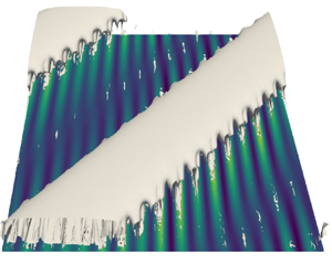
Figure 9. Snapshots of the flow at different times $T$. From left to right and top to bottom: $T=200, 400,600,800,900$. Isosurfaces of the $\lambda _2$-criterion, $\lambda _2=-10^{-5}$ for the two first rows, $-10^{-4}$ for the third and fourth rows and $0.25$ for the last row. The contours depict the streamwise velocity at the wall. The flow is from bottom to top, and left to right. For the sake of clarity, only half the channel is shown.

Meanwhile, at $t \approx 100$, the mode $(0,16)$ starts oscillating with a period $T_0 = 47$. The period of the oscillations is in good agreement with that analytically predicted from (3.8), namely $2{\rm \pi} /(\beta W_0) = 46.58$, hinting at the presence of the modified lift-up described previously. Note that these oscillations can be observed only on this high-wavenumber mode, whereas other streamwise-invariant Fourier modes such as $(0,1)$ (see figure 8) does not display an initial oscillatory phase. A possible reason for this behaviour is that both the target time at which maximum transient growth is recovered, $T_{opt}$, and the oscillation period, $T_0$, are much larger for small spanwise wavenumbers. Furthermore, for $(0,16)$, it can be found that $T_{opt} = 100$ and $T_0 = 47$ whereas $T_{opt} = 615$ and $T_0 = 639$ for the $(0,1)$ mode, which is too large a period to be observed during the linear phase of the perturbation evolution.

After $t\approx 280$, the $(0,16)$ mode exhibits exponential growth, characteristic of a secondary instability. At $t\approx 520$, the $(0,16)$ mode becomes more energetic than the primary one. At the same time, a sharp increase in the kinetic energy indicates that the first step of transition to turbulence has initiated. This translates into a change in the topology of the mode characterised by the onset of near-wall streamwise-elongated coherent structures, shown in figure 9 (second and third rows from the top). These streaky structures are characterised by a large spanwise wavenumber, $\beta =-9.6$, corresponding almost exactly to $16$ times the fundamental spanwise wavenumber $\beta _0$ (namely, $\beta =16\beta _0= -9.6$).

In this transition phase, energy is taken from the 3-D TS wave and transferred to these oblique waves (see figure 9, second and third rows from the top) ultimately leading to the disappearance of the TS wave. As can be seen in figure 10, showing the spatiotemporal evolution of the streamwise (left) and spanwise (right) components of the velocity, these streaky structures are not streamwise independent and are oriented with an angle $\phi = 9^\circ$ with respect to the streamwise direction, almost perpendicular to the initial 3-D TS wave. Note also how the first phase of the transition leads to the decrease of the spanwise velocity component, confirming the streaky nature of the structures.

Figure 10. Spatiotemporal evolution of the streamwise (a,c) and spanwise (b,d) components of the velocity at $x=0$ and $y=-0.85$. For visualisation purposes, the first (second) phase of the transition is depicted separately in the first (second) row.

At $t = 650$, the kinetic energy reaches a plateau for $E = 3\times 10^{-3}$ as the secondary instability saturates (see figure 7). Ultimately, tertiary instability triggers, at $t\approx 800$, a dramatic increase in the friction Reynolds number, indicating the breakdown into a fully turbulent state. This final transition can be linked to the $(0,1)$ mode, as suggested by its sudden growth at such time. Note that this growth is not specific to the $(0,1)$ mode and seems to be shared by all the streaky modes from $(0,1)$ to $(0,9)$ (see figure 8), demonstrating that this behaviour is somewhat general for the streamwise-independent modes and not strictly linked to the domain size. The nature of this final instability is quite complex: it is highly nonlinear as indicated by the growth of all these spatial Fourier modes. It also and appears to be, to some extent, related to streak instability. Figure 10(c,d) depicts streaky structures which, quite interestingly, have lost their orientation and are now aligned with the streamwise direction. The streak instability can be observed at time $t\approx 700$ in the two bottom rows of figure 9 and in the bottom left frame of figure 10.

Quite notably, this transition scenario is fundamentally different from the usual transition scenario in channel flows. Indeed, supercritical transition to turbulence in channel flow is well documented in the no-slip case (Zang & Krist Reference Zang and Krist1989; Schmid & Henningson Reference Schmid and Henningson2001): after an initial exponential growth phase, secondary instability of a subharmonic mode appears. The interaction between the TS wave and the secondary modes leads to a peak–valley structure (Herbert Reference Herbert1985; Asai & Nishioka Reference Asai and Nishioka1989), which, in turn, results in the formation of a staggered pattern of $\lambda$-vortices. Then, $\lambda$-vortices subsequently develop into hairpin vortices that will ultimately breakdown into turbulence. In the slip case, with a homogeneous Navier slip boundary condition, Picella et al. (Reference Picella, Robinet and Cherubini2019) have shown that a delay of the laminar–turbulent transition is possible, but the nature of the instability mechanisms remains virtually the same.

In the present case, the shear misalignment of the base flow appears to have a dramatic effect on the transition scenario. Similarly to what we have reported concerning the primary instability, it might originate a new secondary instability mechanism, which would be investigated in the next subsection. If these cross-flow-related secondary modes have higher growth rates than the subharmonic modes leading to $\lambda _2$ vortices (Herbert Reference Herbert1985), the secondary phase of transition would be dominated by cross-flow-related mechanisms.

As observed in swept flows (Serpieri Reference Serpieri2018), during this secondary phase, oblique waves appear and eventually, through nonlinearities, saturate. The saturated cross-flow vortices contain several strong shear layers, which can, under certain circumstances, further destabilise. The most common instability mechanism observed in such flows (Bippes Reference Bippes1990, Reference Bippes1999) involves the shear layer at the bottom of the vortex, created from the circulation of high-speed fluid towards lower velocities region near the wall.

In the present case, the slip boundary conditions reduce the efficiency of this mechanism by lowering the wall-normal velocity gradients near the walls. Instead, the flow keeps accelerating in the spanwise direction until it reaches a neighbouring vortex, thus creating stagnation points and strong shear layers in the spanwise direction. Transient growth in this region leads to the formation of streaks (Guegan, Huerre & Schmid Reference Guegan, Huerre and Schmid2007) aligned with the streamwise direction. Streak instability concludes the transition to turbulence.

This scenario of transition will be corroborated in the next subsection, by means of secondary stability analysis and comparison with DNS.

5.2. Floquet stability analysis

In an effort to provide a more qualitative description of the secondary phase of the transition, a secondary stability analysis, based on Floquet theory, is carried out. This method has been applied to both channel flows (Herbert Reference Herbert1983) and 2-D boundary layers (Herbert Reference Herbert1985) for which it has successfully predicted the secondary instability of a 2-D TS wave. An extension to 3-D base flows was proposed and applied most notably to swept wings (Fischer & Dallmann Reference Fischer and Dallmann1991; Janke & Balakumar Reference Janke and Balakumar2000; Liu, Zaki & Durbin Reference Liu, Zaki and Durbin2008). Secondary stability equations in a velocity-vorticity formulation can be found in Fischer & Dallmann (Reference Fischer and Dallmann1991). A primitive variables formulation for 2-D base flows only, can be found in Schmid & Henningson (Reference Schmid and Henningson2001).

In this work, due to the three-dimensionality of the problem under consideration, we use a formulation of Floquet theory and subsequent modal expansion somewhat different (but nevertheless equivalent) from those used in these articles. In the study of Herbert (Reference Herbert1983), the Squire theorem ensures a 2-D initial perturbation while, for swept flows cases, an initial 3-D perturbation should be considered. For this reason, Floquet theory for swept flows is usually applied in a rotated frame aligned with the 3-D wave direction of propagation, thus effectively reducing the base flow to two dimensions. Precisely, the base flow for secondary stability analysis is constructed as a superposition of an unstable mode and the laminar flow profile such as

(5.1)\begin{equation} \boldsymbol{U}_1(x,y,t) = \boldsymbol{U}_0(y) + A\boldsymbol{\hat{u}}^{TS}(y)\exp({{\rm i}\alpha_0x + {\rm i}\beta_0 z -{\rm i}\omega_0t}) \end{equation}

with $A$ the amplitude of the unstable 3-D TS wave obtained from linear stability analysis. Considering that the TS wave moves at the velocity $c_x$ and $c_z$ in the $x'$ and $z'$ directions, respectively, the time dependence of the base flow is removed when the moving frame $(x',z') = (x-c_xt, z-c_zt)$ is considered. Linearising the NS equations around this new base flow in the co-moving frame leads to a system of ordinary differential equations (see Appendix C) with $2{\rm \pi} /\alpha _0$-periodic and $2{\rm \pi} /\beta _0$-periodic coefficients in the $x$- and $z$-directions, respectively. Thus, the Floquet theorem is applied in both the streamwise and spanwise directions:

(5.2)\begin{equation} \boldsymbol{q_1}(x',y,z',t) = \boldsymbol{\tilde q}(x',y,z') \operatorname{e}^{\gamma x'} \operatorname{e}^{\mu z'} \operatorname{e}^{\sigma t} \end{equation}

with $\gamma = \gamma _r + {\rm i}\gamma _i$ and $\mu = \mu _r + {\rm i}\mu _i$ the Floquet parameters in the streamwise and spanwise directions. Then, $\boldsymbol {\tilde q}(x',y,z')$ is Fourier transformed in both the $x'$- and $z'$-directions and introducing the detuning factors $\epsilon = \gamma _i/\alpha _0$, $\delta = \mu _i/\beta _0$, the general form of the solution can be expressed as

(5.3)\begin{align} \boldsymbol{q_1}(x',y,z',t)& = \exp({\sigma t})\exp({\gamma _r x'}) \exp({\mu_r z'}) \sum_{m,n={-}\infty}^{+\infty} \boldsymbol{\tilde q}_{m,n}(y) \exp({\rm i}\alpha_0(m + \epsilon)x' \nonumber\\ &\quad + {\rm i}\beta_0(n + \delta)z') . \end{align}

When a numerical solution is sought, the modal expansion (5.3) needs to be truncated, usually with the lowest possible number of modes. Unfortunately, reaching the spanwise wavenumbers observed in the DNS would require a large number of modes in the $z'$-direction, which make the problem too computationally expensive. In order to relax this constraint, the modal expansion in the spanwise direction is reduced to only one mode by fixing $n$ and $\delta$ and introducing $\beta _1 = \beta _0(n + \delta )$, which represents the effective secondary spanwise wavenumber. Since $n \in \mathbb {Z}$ and $-1/2 < \delta \leq 1/2$, the quantity $n+\delta$ spans all real numbers bijectively such that every spanwise wavelength is accessible through a unique choice of $n$ and $\delta$.

Temporal stability is investigated, thus $\gamma _r=\mu _r=0$ and the real part of $\sigma$ indicates the growth rate of the secondary instability. Finally, the modal decomposition (5.3) reduces to

(5.4)\begin{equation} \boldsymbol{q_1}(x',y,z',t) = \exp({\sigma t})\exp({{\rm i}\beta_1 z'})\sum_{m={-}\infty}^{+\infty} \boldsymbol{\tilde q}_{m}(y) \exp({{\rm i}\alpha_0(m + \epsilon)x'}) . \end{equation}

Introducing (5.4) into the linearised NS equations leads to an infinite set of equations which, once truncated, can be recast in an eigenvalue problem likewise the primary stability problem.

All the results given here are obtained with the lowest possible truncation that is ${m=0,1}$ in the subharmonic ($\epsilon =1/2$) cases and $m=-1,0,1$ for the fundamental ($\epsilon = 0$) and detuned ($0 < \epsilon < 1/2$) modes. For the sake of clarity, the derivation of the secondary stability equations and the eigenvalue problem is fully detailed in Appendix C.

In both classic channel and boundary layer flows, fundamental and detuned waves play a limited role in the transition process (Herbert Reference Herbert1983, Reference Herbert1985) as subharmonic instabilities have stronger growth rates. However, this might not be true in our configuration, due to the strong asymmetry present in the base flow.

The dependence of the growth rate of the most unstable mode on the detuning factor is investigated in figure 11, for $Re=12\,000$. A strong secondary growth rate can be reached for detuned modes and large spanwise wavenumbers, in the range of those recovered for the primary cross-flow instability. The maximum secondary growth rate is $\sigma _r = 0.0230$ for $\epsilon = 0.23$ and $\beta _1=-8$ but the instability region is quite large and similar growth rates can be reached for larger $\beta _1$. Precisely, the growth rate corresponding to the spanwise wavelength observed in the DNS (namely, $\beta = -9.6$), is equal to $\sigma _r = 0.020$.

Figure 11. (a) Growth rate $\sigma _r$ of the most unstable mode as a function of the spanwise wavenumber $\beta _1$ for ${\epsilon =0}$ (fundamental), $\epsilon = 0.22$ (detuned) and $\epsilon = 1/2$ (subharmonic). (b) Contour plot of the growth rate $\sigma _r$ of the most unstable mode for $Re=12\,000$ as a function of both the detuning factor $\epsilon$ and the spanwise wavenumber $\beta _1$. Black dot corresponds to the maximum growth rate obtained for $\epsilon =0.23$ and $\alpha =-8$ whereas the black line denotes the $\sigma _r = 0.02$ isocontour (corresponding to the growth rate found from the DNS). The broken line denotes the $\sigma _r = 0.015$ isocontour and allows the identification of secondary maxima.

The spectrum obtained for $Re=12\,000$, $\beta _1 = -9.6$, $\epsilon = 0.23$ and $A = 10^{-5}$, shown in figure 12, exhibits three unstable and one marginally unstable mode. All the modes share a similar structure: the $m=0$ mode, yielding an effective streamwise wavenumber $\alpha = \epsilon \alpha _0 = 0.16$, is dominant in comparison with the $m=-1$ and $m=1$ modes. The wavenumber in the streamwise direction is too small to be retrieved in the computational domain thus explaining, to some extent, the onset of streaky structures. The eigenvalues associated to these modes are summarised in table 2. Considering the dominant $m=0$ mode, frequencies in the laboratory frame are retrieved through the following equation:

(5.5)\begin{equation} \sigma_i^{0} = \sigma_i^{TS} - \beta_1 c_z - \alpha_0 \epsilon c_x. \end{equation}

Figure 12. Secondary instability spectra for $Re=12\,000$, $\beta _1=-9.6$, $A = 10^{-5}$ and $\epsilon =0.23$. Eigenvalues are coloured according to their respective Fourier mode. The values of the frequency and growth rate of the four most unstable modes are given in table 2.

Table 2. Most unstable eigenvalues of the secondary stability analysis for $Re=12\,000$, $\beta _1 = -9.6$, $\epsilon = 0.23$ and $A = 10^{-5}$. For a single mode, two frequencies, $\sigma _i^{TS}$ and $\sigma _i^{0}$, are given: the former is the frequency of the mode in the frame moving with the TS wave whereas the latter corresponds to the frequency in the laboratory frame.

For the four most unstable modes, secondary perturbations are reconstructed based on (5.3). A slice of these modes in the $y\unicode{x2013}z$ plane is provided in figure 13, showing that they share a rather similar structure. In the spanwise direction, one can see alternated high and low streamwise-velocity patches. The streamwise velocity component is one order of magnitude higher than the cross-flow components, and is strongly localised in the region where the amplitude of the TS wave reaches a maximum. Cross-flow components form vortical structures concentrated near the walls and similar to those found for cross-flow instabilities. More precisely, mode 1 consists of oblique vortices together with oblique streaky structures for the streamwise velocity component. Modes 2 and 4 are almost identical besides a phase shift. One can also observe a stagnation point near the wall at $z=0.58$ for mode 2. Mode 3 appears peculiar as its vortices sit on top of a region of low velocity. For all these modes, the vortices push high-momentum fluid towards the wall where, due to the slip boundary conditions, it is strongly accelerated in the spanwise direction. When this high-momentum flow reaches the neighbouring vortices, it is re-ejected upwards back in the flow, creating stagnation points and strong spanwise shear layers in the process.

Figure 13. Slice at $x=L_x/2$ of the reconstructed secondary perturbations of the four most unstable modes for $Re=12\,000$, $\beta _1 = -9.6$, $\epsilon = 0.23$ and $A = 10^{-5}$. From top to bottom and left to right, modes are ordered from the most unstable to the least unstable. The contour plot represents the streamwise velocity disturbance whereas the quiver plot shows the $v$–$w$ cross-flow.

The main features of the most unstable modes recovered by Floquet analysis are compared with those observed in the DNS in table 3. For the DNS, the secondary growth rate is extracted from figure 8. A good agreement can be found between the values. A comparison of the spatial structure of the secondary perturbations obtained from the DNS and some of the modes obtained by secondary stability analysis is provided in figure 14. Snapshots of the flow are taken at $x=L_x/2$ and $t=500$. Both the base flow and the initial TS wave are subtracted from the snapshot to retrieve the secondary perturbations. The snapshot is then divided into portions of size $2{\rm \pi} /\beta _1$ to isolate vortical structures.

Table 3. Comparison between spanwise wavenumbers and growth rates obtained from the DNS and from secondary stability analysis.

Figure 14. Comparison between snapshots extracted from the DNS (a,c) and secondary stability modes (b,d): mode 1 (a,b) and mode 3 (c,d). Secondary perturbations from the DNS are extracted from snapshots taken at $t=500$, by subtracting the base flow and the primary disturbance. The contour plot represents the total streamwise velocity disturbance whereas the quiver plot shows the $v$–$w$ cross-flow.

The spatial structures compare rather well, although for mode 1 (top row), one can observe that in the DNS the counter-rotating vortices are located rather farther from the wall. Regarding mode 3, its location in the wall-normal direction can be retrieved despite the size of the vortex is slightly smaller. These discrepancies could be explained from different factors: as can be seen, secondary stability analysis yields a range of unstable spanwise wavenumbers which includes the main wavenumber observed in the DNS. The growth rates are in perfect agreement. The small discrepancy found between the frequencies could arise from the fact that the shape assumption is likely not completely valid and the mean flow is slightly distorted during the transition. In addition, only the frequency of the dominant mode $m=0$ was considered whereas, formally, each mode of the Floquet expansion has its own frequency in the laboratory frame.

6.1. Overview of the transition

The second transition scenario is initiated injecting on the base flow the cross-flow unstable mode with $(\alpha _0, \beta _0) = {(0.2,-6)}$. The time evolution of the kinetic energy evolution and friction Reynolds number is provided in figure 15, whereas figure 16 depicts the evolution of the spectral energy for several Fourier spatial modes along with spatiotemporal plots.

Figure 15. Evolution of the disturbance kinetic energy density (a) and $Re_{\tau }$ (b) for the cross-flow transition scenario. The dashed line has a slope $2\omega _r$ where $\omega _r \approx 0.003267$ is the growth rate of the most unstable perturbation found with the linear stability analysis.

Figure 16. (a) Time evolution of the Fourier modes $(1,1)$, $(2,0)$, $(7,0)$ and $(0,1)$ for the cross-flow transition scenario. The dashed line corresponds to the exponential primary growth rate. (b) Spatiotemporal evolution of the streamwise component of the velocity at $x=0$ and $y=-0.85$.

At first, exponential growth of the disturbance kinetic energy is observed in figure 15. Note that the slope of the curve corresponds to twice the growth rate $\omega _r = 0.0033$ retrieved from linear stability analysis. After $t=600$, the kinetic energy starts saturating at $E \approx 1.8\times 10^{-3}$. This saturation most likely arises from stabilising nonlinear effects and is also observed in a cross-flow-induced transition for swept flows. As shown in the first snapshot of figure 17, apart from slight deformations near the walls due to the boundary conditions, the shape of the quasi-stationary ($\omega _i = 0.0225$) cross-flow vortices does not evolve much during this phase.

Figure 17. Snapshots of the flow at $T=900,1010,1030,1060,1080,1150$ (from top to bottom and left to right). Isosurfaces of the $\lambda _2$-criterion, $\lambda _2=-10^{-5}$ (a,b), $\lambda _2=-10^{-4}$ (c,d) and $\lambda _2=-10^{-1}$ (e, f), respectively, and contours of the streamwise velocity at the wall. For the sake of clarity, only half the channel is shown.

In the meantime, it can be seen from figure 16(a) that the mode $(2,0)$ also experiences strong energy growth. Since the mode is linearly stable and is not expected to undergo strong transient growth, only nonlinear mechanisms could explain this growth. Nonlinear forcing of the mode $(2,0)$ by the initial perturbation is possible as it can be observed in an oblique waves transition scenario for a boundary layer (Schmid & Brandt Reference Schmid and Brandt2014). Usually, the $(2,0)$ mode is damped and not very receptive to forcing, meaning it is not relevant in the transition scenario. For 3-D flows, El-Hady (Reference El-Hady1989) demonstrated that resonant wave triads play an important role in the stability due to the large number of interaction between the possible instabilities.

At $t = 1000$, the top of the vortices start oscillating in the streamwise direction (see figure 17b,c). This can also be seen on the spatiotemporal plot of figure 16(b), where one can note the much higher frequency of the secondary instability. This secondary instability can be traced back to the Fourier mode $(7,0)$ in figure 16(a). Secondary growth rate can be extracted from the slope of its time evolution and is equal to $\sigma _r \approx 0.084$.

At $t \approx 1050$ (see figure 17d,e), spanwise-independent coherent structures appear as shown in figure 18. These structures appear on top of the cross-flow vortices and seem to be tilted. The bottom snapshot of figure 18 is particularly interesting: on top of the wave-like pattern of the initial disturbance, secondary vortices can be observed. These also appear in the near-wall region between two cross-flow vortices. These vortices are most likely a consequence of the slip boundary conditions: as the fluid is accelerated in the spanwise direction near the walls, strong spanwise shear layers, which are susceptible to further destabilise, are created. Energy is transferred from the cross-flow vortices to the secondary perturbation. Distortion of the base flow, in both streamwise and spanwise directions, is also highly likely.

Figure 18. Cross-flow dynamics at different time $T$. From top to bottom: $T=900,1000,1050, 1060,1080$. The cross-section is taken at the streamwise position $x_s = 15.71$ and only $y \in [-1,-0.7]$ is represented. Isocontours of the $\lambda _2$-criterion [$-1\times 10^{-4} \longleftrightarrow -1\times 10^{-2}$]. Contour plot of the $u$-component of the disturbance velocity. Quiver plot depicts the $(v$–$w)$ cross-flow of the perturbation. White contours represent the magnitude of the velocity $[-5\times 10^{-2}, -3\times 10^{-1}; -5\times 10^{-2}]$.

The remaining part of the laminar–turbulent transition is rather complex as several instability mechanisms get intertwined. In the last two snapshots of figure 17, streaks can be seen developing in the near-wall region, causing the energy growth of the $(0,1)$ Fourier mode in the left frame of figure 16. In figure 18, the vortices described previously have combined to form vortex quadrupoles which create strong recirculation in the flow. Ultimately, the breakdown to turbulence seems to be related to the displacement of high-velocity fluid in the upper part of the channel (fourth snapshot of figure 18) towards lower-velocity regions near the wall (last snapshot of figure 18). In the vicinity of these regions turbulent wedges originate (see figure 16b) which quickly propagate to the whole channel.

6.2. Secondary stability analysis of cross-flow vortices

Due to the presence of several strong shear layers in the primary cross-flow vortices, these are highly likely to destabilise. The observation of the transition scenario also strongly hints at the presence of modal secondary instability mechanisms. In the case of swept flows, numerous efforts on the secondary instability of cross-flow vortices have been performed, albeit, to the best of the authors’ knowledge, always for boundary flows with no-slip boundary conditions. While a short introduction to secondary instability of cross flow vortices is produced in the following, the reader is referred to Saric et al. (Reference Saric, Reed and White2003) for a full review.

One of the first key contribution to this issue has been the work of Malik et al. (Reference Malik, Li, Choudhari and Chang1999) which classified the secondary modes into two main families. Precisely, type-I unstable modes are linked to the velocity gradient of the streamwise component of the velocity in the spanwise direction, whereas type-II modes originate from gradients in the wall-normal direction. Type-I modes are located in the outer part of the primary vortices whereas type-II are situated on top of them. Type-II also tend to have a higher frequency than type-I modes. A third type of mode was identified in studies by Fischer & Dallmann (Reference Fischer and Dallmann1991) and Janke & Balakumar (Reference Janke and Balakumar2000) through Floquet analysis of the cross-flow vortices. This low-frequency type-III mode is linked to nonlinear interactions between stationary and travelling primary modes. These three families of modes have been also experimentally retrieved by Kawakami, Kohama & Okutsu (Reference Kawakami, Kohama and Okutsu1999) and White & Saric (Reference White and Saric2005). Later, using DNS, Wassermann & Kloker (Reference Wassermann and Kloker2002, Reference Wassermann and Kloker2003) showed that co-rotating helicoidal structures superimposed on the upwelling region of the primary vortices were characteristics of the type-I mode. These structures would be convected downwards if the unsteady forcing was switched off, thus confirming the convective nature of the secondary instability as already suggested by Kawakami et al. (Reference Kawakami, Kohama and Okutsu1999) and Koch (Reference Koch2002).

Bonfigli & Kloker (Reference Bonfigli and Kloker2007) also studied the development of the secondary instabilities of cross-flow vortices through the combined use of a spatial DNS and secondary linear stability theory (SLST) based on Floquet theory applied on a saturated primary flow (Malik, Li & Chang Reference Malik, Li and Chang1994; Janke & Balakumar Reference Janke and Balakumar2000; Koch et al. Reference Koch, Bertolotti, Stolte and Hein2000; Koch Reference Koch2002). Growth rates and structures of the type-I and type-III modes were retrieved and good agreement was shown between the two techniques. SLST predicted the instability of type-II modes but these were not observed in the DNS. In the particular case of travelling vortices, type-III modes were not reported as unstable, which was expected since this mode arises from the generation of spanwise modulation induced by the stationary primary vortices. Another key conclusion of this study is the nature of the mechanism behind the secondary instability: both type-I and type-II are found to be related to Kelvin–Helmoltz instabilities. In all cases, the primary flow on which SLST is carried out is paramount and its acquisition is not straightforward as nonlinearities lead to an important distortion of the base flow. The shape assumption no longer holds and Herbert's secondary stability theory cannot be applied directly.

The primary flow can be retrieved by using parabolised stability equations as in Malik et al. (Reference Malik, Li, Choudhari and Chang1999) and Janke & Balakumar (Reference Janke and Balakumar2000), or extracted directly from a saturated DNS (Messing & Kloker Reference Messing and Kloker2004; Bonfigli & Kloker Reference Bonfigli and Kloker2007). Recently, Groot et al. (Reference Groot, Serpieri, Pinna and Kotsonis2018) based their secondary stability analysis on an experimentally acquired primary flow. In any case, the extraction process is quite complex and several issues arise. In swept boundary layers, the orientation of the vortex axis of the cross-flow vortices evolves with the streamwise direction. Consequently, secondary linear stability depends on the position $x=x_{SLST}$ where the primary flow is extracted. This is not the case in our configuration, as a consequence of the choice of a temporal DNS.

As in Bonfigli & Kloker (Reference Bonfigli and Kloker2007) and several others, we introduce a vortex-oriented system $(x_v,y,z_v)$ aligned with the vortex axis of the primary disturbance and moving with it. In this frame, the primary flow $\boldsymbol {Q}_v^0(y,z_v)$ is streamwise independent and periodic in the spanwise direction. In the framework of Floquet theory, it is Fourier expanded in the spanwise direction and takes the following modal form:

(6.1)\begin{equation} \boldsymbol{Q}_v^0(y,z_v) = \sum_{n={-}\infty}^{+\infty} \boldsymbol{\hat{q}}^0_{v,n}(y)\exp({{\rm i}n\beta_vz_v}) \end{equation}

with $\beta _v =\sqrt {\alpha _0^2 + \beta _0^2} \approx \beta _0$ the effective wavelength in the spanwise direction $z_v$. In this framework, the continuity equation reduces to

(6.2)\begin{equation} \partial_y v^0_{v,n} + {\rm i}n\beta_vw^0_{v,n} = 0, \quad \forall n, \end{equation}

directly relating the two cross-flow components of the velocity. Thus, a choice must be made between enforcing continuity and extracting both components from the DNS. Ultimately, this might have a non-negligible effect on the secondary growth rates found from the SLST (Malik et al. Reference Malik, Li and Chang1994; Bonfigli & Kloker Reference Bonfigli and Kloker2007).

To overcome this and other issues of Floquet analysis, here we use a local 2-D stability (Tatsumi & Yoshimura Reference Tatsumi and Yoshimura1990) approach. Several reasons motivate this choice: first and foremost, 2-D local stability theory encompasses Floquet stability theory. In addition, as shown previously, Fourier decomposition in the spanwise direction of the primary flow leads to some difficulties with the continuity equation. In a 2-D framework, this decomposition is not necessary and these issues do not arise. Ultimately, 2-D stability analysis allows to take into account also instabilities spanning multiple cross-flow vortices, whereas other studies only considered a single pattern of the primary flow for their secondary stability analyses.

For carrying out the 2-D secondary stability analysis, the flow is decomposed into the primary state $\boldsymbol {Q}_v^0(y,z_v)$ and a secondary perturbation $\boldsymbol {q}_1(x_v,y,z_v,t)$. Furthermore, the secondary perturbation can be expanded in the following way:

(6.3)\begin{equation} \boldsymbol{q}_1(x_v,y,z_v,t) = \tilde{\boldsymbol{q}}(y,z_v)\exp({{\rm i}\alpha_v x_v - \sigma t}), \end{equation}

where $\alpha _v$ and $\sigma$ are complex numbers representing the streamwise wavelength and the pulsation in the vortex-oriented reference frame, respectively. Both temporal (Malik et al. Reference Malik, Li, Choudhari and Chang1999; Koch et al. Reference Koch, Bertolotti, Stolte and Hein2000; Wassermann & Kloker Reference Wassermann and Kloker2002) and spatial (Janke & Balakumar Reference Janke and Balakumar2000; Bonfigli & Kloker Reference Bonfigli and Kloker2007) approaches have been considered previously. Koch et al. (Reference Koch, Bertolotti, Stolte and Hein2000) found a set of equations relating both frameworks through a generalisation of the Gaster transformation to 3-D flows. For channel flows, a natural choice is to consider a temporal framework. As previously, NS are linearised around this new base flow. Stability equations for 2-D problems can be found, for example, in Loiseau (Reference Loiseau2014).

The primary flow in the vortex-oriented reference frame is shown in figure 19. It was extracted from the DNS at time $t=900$ and $x_{SLST}=15.71$. This flow field can be compared with the flow visualisations from the experiments of Serpieri (Reference Serpieri2018) (see figure 4.14) and with the primary flow resulting from the DNS of Bonfigli & Kloker (Reference Bonfigli and Kloker2007) (see figure 7). The water-wave shape of the streamwise velocity component, characteristic of the cross-flow vortices, is clearly visible. However, the spatial extension of the tip of the wave is smaller than that observed for swept boundary flows, likely because the initial spanwise velocity $W_0$ is weaker. The instability mechanism is similar to that described in Serpieri & Kotsonis (Reference Serpieri and Kotsonis2016): cross-flow vortices generate the circulation of low-momentum flow towards high-momentum regions higher up in the channel and conversely. In the present case, the wall-normal shear is maximum near the walls and not in the vortex core due to the slip boundary conditions. The spanwise velocity gradient reaches a maximum in the low-momentum upwelling region on the outer part of the vortex.

Figure 19. Secondary base flow for the secondary stability analysis. The snapshot is extracted from the DNS at time $t \approx 900$, position $x_{SLST} = 15.71$ and is shown in the vortex-oriented reference frame. (a) Contour plot of the velocity component $U$. Quiver plot of the cross-flow perturbation $(v$–$w)$. (b) Growth rate $\sigma _r$ of the secondary most-unstable modes of cross-flow vortices as a function of the effective streamwise wavenumber $\alpha _v$ in the vortex-oriented frame.

Two-dimensional stability analysis of the previously described primary flow is performed. The evolution of the temporal secondary amplification rates in the vortex-oriented frame as a function of the effective streamwise wavelength is shown in figure 19. The maximum growth rate is equal to $\sigma _r = 0.084$ for $\alpha _v=1.4$. Both the growth rate and the effective streamwise wavenumber are in good agreement with those observed in the DNS. A direct comparison between the characteristics of the secondary instability obtained from the SLST and those extracted from the DNS is provided in table 4.

Table 4. Comparison between secondary instability characteristics obtained from the DNS and from the most-unstable mode of the secondary stability analysis.

All the results from the SLST are obtained in the moving vortex-oriented frame. Values of streamwise wavelengths and frequencies in the laboratory frame can be retrieved by expanding (6.3):

(6.4)$$\begin{gather} \sigma_i^{0} = \sigma_{i,v} - \alpha_v c, \end{gather}$$

(6.5)$$\begin{gather}\alpha_1^{0} ={-}\frac{\alpha_v \beta_0}{k}, \end{gather}$$

(6.6)$$\begin{gather}\beta_1^{0} = \frac{\alpha_v \alpha_0}{k}, \end{gather}$$

where $k = \sqrt {\alpha _0^2 + \beta _0^2}$ and $c$ is the velocity of the cross-flow vortices.

For $Re=12\,000$ and $\alpha _v = 1.4$, two families of eigenmodes could be distinguished and are displayed in figure 20. The first, in the left part of the figure, appears strongly localised on the upwelling of the vortex, a representative feature of type-I modes. Among the several unstable modes, no type-II nor type-III structures could be found. This is not unexpected: type-III modes require interactions with unstable stationary cross-flow vortices. Type-II modes stem from the instability of wall-normal velocity gradients but these are sensibly weaker than their counterparts in swept flows. This could be explained by the combined effect of the absence of an inflection point in the spanwise velocity profile $W_0$ and of the slip boundary conditions. Regarding the second mode, it is slightly less unstable ($\sigma _r = 0.0815$ against $\sigma _r = 0.0827$ for the previous mode) and has a smaller frequency ($\sigma _i = 0.4439$ against $\sigma _i = 0.5319$) but presents a strong resemblance with the left snapshot, second row of figure 17 from the DNS (see also figure 18b,c). The corresponding contour plot in figure 20 also displays the existence of a shear layer in the spanwise direction at the top of the cross-flow vortices, right at the location where the spanwise independent structures will develop. Also of interest is the fact that these two perturbations are fundamental: they have the same spatial periodicity than the secondary base flow.

Figure 20. Most unstable secondary modes found for $Re=12\,000$, $\alpha _v=1.4$ (a,b) corresponding respectively to $\sigma = 0.0827 -0.5319 { i}$ (a) and $\sigma = 0.0815 - 0.4439 {i}$ (b) and for $\alpha _v=1$ (c). Slice in the $(y\unicode{x2013}z)$ plane. The contour plots depict the streamwise velocity perturbation whereas the quiver plots represent the cross-flow dynamics.

The most-unstable mode for $\alpha _v=1$ is shown in figure 20(c) and is similar to the first mode for $\alpha _v=1.4$. It is also a type-I mode but, in the present case, a phase shift appears between each cross-flow vortex. The periodicity of the secondary mode is now three times the periodicity of the primary cross-flow vortices, indicating the existence of detuned modes.