


1. Introduction
Rotating convective flows are of fundamental importance in many natural systems, such as in the atmospheres of planets and inside the stars. These geophysical and astrophysical systems are large in scale, complex in dynamics, and far from the reach in laboratory measurements. Nevertheless, the two most important factors in these systems, i.e. convection and rotation, have been explored over many years by a simplified model system – the rotating Rayleigh–Bénard convection (RRBC), where a rotating fluid layer is heated from below and cooled from above (Chandrasekhar Reference Chandrasekhar1981). In RRBC, convection is driven by the buoyancy force, which is caused by the applied temperature difference  $\Delta T$ across the fluid layer. Its strength is characterized by the Rayleigh number $Ra=\alpha g\Delta T H^3/(\nu \kappa )$. Rotation introduces two effects in the system, i.e. the effects of the Coriolis force and the axisymmetrically distributed centrifugal force, which can be quantified by the Rossby number $Ro=U_{\!f\!f}/(2\varOmega H)$ and the Froude number $Fr_R=\varOmega ^2R/g$, respectively. Here, $\varOmega$ is the rotation speed antiparallel to the gravity $g$ and $U_{\!f\!f}=\sqrt {\alpha g\Delta TH}$ is the free-fall velocity. The flow domain is characterized by the depth $H$ and radius $R$.
$R$.  $\alpha$, $\nu$ and $\kappa$ are the thermal expansion coefficient, the kinematic viscosity and the thermal diffusivity of the working fluid, respectively.
For Earth's parameters, the Froude number is of the order of  $10^{-3}$. Thus, the centrifugal effect is often neglected in RRBC, and the Coriolis effect has attracted much attention instead (see, e.g. the review articles by Stevens, Clercx & Lohse (Reference Stevens, Clercx and Lohse2013), Kunnen (Reference Kunnen2021) and Ecke & Shishkina (Reference Ecke and Shishkina2023)). The effects of the Coriolis force are twofold. In the bulk region of isothermal flows, the balance between the Coriolis force and the pressure gradient dominates the dynamics, i.e.
 \begin{equation} 2\boldsymbol{\varOmega} \times \boldsymbol{u}={-}\boldsymbol{\nabla}p \quad \xrightarrow{\boldsymbol{\nabla}\times({\cdot})}\quad \partial_z\boldsymbol{u}=\boldsymbol{0}. \end{equation}
This so-called Taylor–Proudman (TP) constraint (Proudman Reference Proudman1916; Taylor Reference Taylor1923) makes the flow two-dimensional. However, in RRBC with temperature gradient, the TP constraint is replaced by the thermal wind balance, i.e.
 \begin{equation} 2\boldsymbol{\varOmega} \times \boldsymbol{u}={-}\boldsymbol{\nabla}p+\alpha gT\boldsymbol{e_z} \quad \xrightarrow{\boldsymbol{\nabla}\times({\cdot})}\quad \partial_z\boldsymbol{u}=\frac{\alpha g}{2\varOmega}\boldsymbol{e_z}\times\boldsymbol{\nabla}T. \end{equation}
It can be seen that the effect of the temperature gradient is to violate the TP constraint and the resulting convective motion tends to make the flow three-dimensional-like (King et al. Reference King, Stellmach, Noir, Hansen and Aurnou2009; Grooms et al. Reference Grooms, Julien, Weiss and Knobloch2010). The competition between the effects of the Coriolis force and the temperature gradient makes the RRBC system exhibit rich and complex flow phenomena (Sprague et al. Reference Sprague, Julien, Knobloch and Werne2006; Julien et al. Reference Julien, Rubio, Grooms and Knobloch2012; Cheng et al. Reference Cheng, Madonia, Aguirre, Andrés and Kunnen2020). On the other hand, in the boundary layer, the effect of thermal wind balance is replaced by the Ekman pumping, which changes the flow dynamics there (Kunnen, Geurts & Clercx Reference Kunnen, Geurts and Clercx2010; Kunnen et al. Reference Kunnen, Stevens, Overkamp, Sun, van Heijst and Clercx2011b; Plumley et al. Reference Plumley, Julien, Marti and Stellmach2016) and enhances the vertical transport efficiency (Zhong et al. Reference Zhong, Stevens, Clercx, Verzicco, Lohse and Ahlers2009; Stevens, Clercx & Lohse Reference Stevens, Clercx and Lohse2010; Weiss et al. Reference Weiss, Stevens, Zhong, Clercx, Lohse and Ahlers2010; Weiss, Wei & Ahlers Reference Weiss, Wei and Ahlers2016).
Recently, the centrifugal effect has also received some attention. The centrifugal force tends to generate accumulations of hot fluid parcels at the cell centre and cold ones around the sidewall. After the centrifugal effect sets in, the flow states can be divided into a weak- and a strong-centrifugal regime (Hu, Xie & Xia Reference Hu, Xie and Xia2022). In the weak-centrifugal regime, the radial diffusive motions of hot and cold columns are enhanced (Noto et al. Reference Noto, Tasaka, Yanagisawa and Murai2019; Ding et al. Reference Ding, Chong, Shi, Ding, Lu, Xia and Zhong2021); whereas in the strong-centrifugal regime, the columns are squeezed by the strong centrifugal force to form a large hot coherent structure at the cell centre (Horn & Aurnou Reference Horn and Aurnou2018, Reference Horn and Aurnou2019).
In astronomy, a celestial body is often coupled with other planets or stars, such as the Earth–Moon system and the binary star systems. Therefore, besides the self-gravity  $g$, the convective flows in a planet are often affected by an external gravity (i.e. the tidal force), which is exerted by the nearby planet or star. The most striking example in the solar system is Jupiter's moon, Io. The dramatic tidal force from Jupiter causes Io's solid surface to bulge up and down by many 10s of metres (Spencer & Schneider Reference Spencer and Schneider1996). For comparison, the height of the tides in the Earth's ocean is only $O(10)$ m. This tidal force changes the dynamics of the partial-melt asthenosphere inside Io, and makes Io the most volcanically active world in the solar system (Hamilton et al. Reference Hamilton, Beggan, Still, Beuthe, Lopes, Williams, Radebaugh and Wright2013; Steinke et al. Reference Steinke, van Sliedregt, Vilella, van der Wal and Vermeersen2020). Io is tidally locked to Jupiter. Thus, on Io's surface, there is always a nearest (the subjovian point) and a farthest (the antijovian point) point to Jupiter. The theories, which treat Io as essentially a solid body (Tyler, Henning & Hamilton Reference Tyler, Henning and Hamilton2015), predict that the volcanoes are most active near the subjovian and antijovian points (Segatz et al. Reference Segatz, Spohn, Ross and Schubert1988), which is in qualitative agreement with the observations. Unexpectedly, a detailed investigation of the global distribution of volcanoes on Io revealed a $30^\circ \unicode{x2013}60^\circ$ offset of the volcano cluster centres from the tidal axis (Hamilton et al. Reference Hamilton, Beggan, Still, Beuthe, Lopes, Williams, Radebaugh and Wright2013; Steinke et al. Reference Steinke, van Sliedregt, Vilella, van der Wal and Vermeersen2020). This was partially explained by the assumption of the existence of a magma ocean inside Io, in which case the fluidity allows the Coriolis force to take effect (Tyler et al. Reference Tyler, Henning and Hamilton2015).
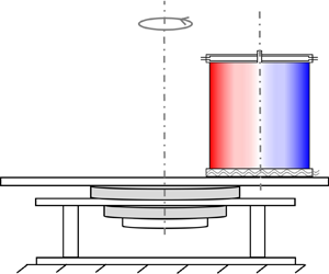
To model the tidal effects in the laboratory, we performed a novel experiment in RRBC, where the convection cell was shifted away from the rotation axis by an offset distance  $d$ (see figure 1a). With the rotating frame set at the cell centre, the centrifugal force that is felt by a fluid parcel can be decomposed into an axisymmetrical part $\varOmega ^2\boldsymbol {r}$ and a directed one $\varOmega ^2\boldsymbol {d}$. The later is characterized by a new Froude number $Fr_d=\varOmega ^2d/g$. In a recent paper (Hu et al. Reference Hu, Huang, Xie and Xia2021), it has been reported that the symmetry of the system is broken by this directed centrifugal force, resulting in a flow bifurcation. Specifically, the hot and cold fluid parcels are separated by $\varOmega ^2d$ and condensed, respectively, near the nearest and farthest points to the rotation axis. Moreover, the condensation centres also show an offset from the nearest and farthest points. These behaviours are quite similar to the key features of the volcano distributions on Io described above, the reason of which is that this directed centrifugal force plays a role similar to the tidal force in Io.

Figure 1. (a) A sketch of the off-centred experimental set-up. The convection cell is shifted away from the rotation axis with an offset distance  $d$. The top view on the left-hand side shows that the centrifugal force $\boldsymbol {F}_c$ felt by a fluid parcel can be decomposed into an axisymmetrical part $\varOmega ^2 \boldsymbol {r}$ and a directed one $\varOmega ^2 \boldsymbol {d}$. (b) A sketch shows the azimuthal positions of the sidewall thermistors and the physical meanings of the quantities that obtained from the TEE method. The azimuthal positions of the coldest ( $\phi _c$) and hottest ( $\phi _h$) points are defined relative to the farthest ( $\phi =0$) and nearest ( $\phi ={\rm \pi}$) points, respectively. The vertical plane that defined by the coldest and hottest positions does not pass through the centre of the convection cell and shows an offset distance $-l$. See § 2.2 for further explanation.
The results in Hu et al. (Reference Hu, Huang, Xie and Xia2021) mainly concern the properties with and without the offset effects, namely, after the offset effects set in, the flow bifurcates and correspondingly, the global heat transport starts to enhance at an onset Froude number  $Fr_{d,c}$ and then reaches an optimal state at $Fr_{d,max}$. Whereas the present work focuses on the local properties after the offset effects set in, showing different features before and after $Fr_{d,max}$. For example, the turbulent bulk flow, which is full of columns near onset, turns into a laminar state with ‘empty’ bulk at around $Fr_{d,max}$. This transition can be understood by an equivalent tilted RRBC system. On the other hand, the vertical temperature variations of the hot and cold coherent structures first decrease with $Fr_d$ and then start to increase at $Fr_{d,max}$, implying that these structures are mostly uniform along the vertical direction at $Fr_{d,max}$. Their temperature contrasts, following a linear behaviour near onset, show a deviation from this linear dependence when $Fr_d>Fr_{d,max}$. Moreover, the effect of $Fr_R$ has been investigated in the present study, which shows that the joint action of $Fr_R$ and $Fr_d$ results in a symmetry breaking in the centrifugal effect for the hot and cold fluid parcels; whereas only the effect of $Fr_d$ was studied in Hu et al. (Reference Hu, Huang, Xie and Xia2021).
The remainder of this paper is organized as follows. The experimental set-up and the sidewall temperature analysis method are introduced in § 2. In the results section, we first briefly review the global features of this off-centred system in § 3.1, and then introduce the local properties of the bulk flow in § 3.2. As for the coherent structures in the sidewall region, their mean properties are first shown in § 3.3 and in the following section (§ 3.4), their local properties are investigated. Finally, we summarize our findings in § 4.
2. The experimental set-up and method
2.1. The experimental set-up and parameters
The structure of the rotating table has been described in detail in Hu et al. (Reference Hu, Xie and Xia2022). Here, only the key features and the differences with the centred experiments are introduced. The convection cell and all the other related equipment were seated on a large aluminium plate, whose diameter is  $1500$ mm. As sketched in figure 1(a), the convection cell was shifted away from the rotation axis with an offset distance $d$, which is normalized by the cell's radius $R=97.1$ mm as $\gamma =d/R$. In order to change the offset distance $d$ freely, a pair of sliding rails were used, above which the convection cell was seated. Seven different sets of experiments were performed, with the normalized value of $\gamma =$ 0.00, 0.21, 0.82, 1.00, 1.65, 3.50 and 5.15. For $\gamma \leq 1.65$, the rotation speed changed from 6 r.p.m. to 60 r.p.m., resulting in the Rossby number $Ro$ and the Froude number $Fr_R$ covering the range of $0.045\leq Ro \leq 0.44$ and $0.004\leq Fr_R \leq 0.39$, respectively. For safety reasons, the rotation speed was only pushed to 52 r.p.m. (40 r.p.m.) for $\gamma =3.50$ (5.15). Thus, the new Froude number $Fr_d$ varied from $8\times 10^{-4}$ to 1.03.
This off-centred configuration not only makes the rotational inertia extremely large but also makes the whole rotational system unbalanced, which challenges the performance of our rotating table, especially for the case with large  $\gamma$ at large rotation speed. Thus, before the experiments, great care was taken to level the rotating table within $10^{-4}$ rad and to ensure system integrity. For safety reasons, the ramp-up speed of the table was set at 2 r.p.m. min $^{-1}$ for each experiment. This extremely slow speed allows us to deal with any emergent events (if they happen). A weight balance was fixed at the opposite side of the sliding rails. If the mass of the balance was not enough, some noise, which was absent in the centred experiments, could be heard during the ramp-up process. This noise essentially arises from the residual imbalance of the system. In this case, the experiment was stopped immediately and the mass of the balance was increased gradually. This procedure was repeated until the noise vanished, according to which we judged that the system was almost in balance. A Hall sensor and a camera were further used to monitor the working state of the rotating table.
The experimental set-up for heat transport measurements is similar to the one used in the standard Rayleigh–Bénard experiments. The cylindrical convection cell, which was filled with degassed and deionized water, has an aspect ratio  $\varGamma =2R/H=1$ with its height $H=194.2$ mm. The heat flux $q$ was applied to the hot bottom plate by heating nichrome wires, and then extracted by the cold top plate, whose temperature was regulated by a circulating water bath. In each plate, four thermistors were used to monitor their temperatures $T_{bot}$ and $T_{t\!o\!p}$, respectively. During the experiments, the temperature difference $\Delta T=T_{bot}-T_{t\!o\!p}$ was kept at $16.0$ K with an accuracy better than 0.1 K, resulting in a fixed Rayleigh number $Ra=4.4\times 10^9$. A small thermistor was used to measure the bulk temperature $T_{bulk}$ at the cell centre. In the sidewall, $24$ thermistors were distributed in three horizontal rows with altitudes $H/4,\ H/2$ and $3H/4$ from the bottom plate and in eight vertical columns equally spaced azimuthally. Their azimuthal positions $\phi _i=i{\rm \pi} /4\ (i=0, 1,\ldots, 7)$ are defined in figure 1(b), with $\phi _0$ corresponding to the farthest point to the rotation axis. All the thermistors used to measure temperatures were calibrated individually and separately in a temperature-controlled water bath, with a temperature accuracy better than 0.01 K. A copper basin was placed under the bottom plate to compensate the heat leakage from the bottom plate. Its temperature was regulated to $T_{bot}\pm 0.05$ K by a program. The convection cell was wrapped by several layers of Styrofoam to reduce the heat leakage from the sidewall, and then put into a home-made thermostat to minimize the influence of the fluctuating surrounding temperature. The temperature stability of the thermostat was better than 0.1 K. The Prandtl number $Pr=\nu /\kappa$ was fixed at $4.34$, corresponding to 40.0 $^\circ$C bulk temperature. The heat transport efficiency was quantified by the Nusselt number $Nu =q/(k \Delta T/H)$, with $k$ the thermal conductivity of water.
The flow fields were visualized by particle image velocimetry (PIV) measurements (Xia, Sun & Zhou Reference Xia, Sun and Zhou2003; Sun, Xia & Tong Reference Sun, Xia and Tong2005) for  $\gamma =$ 0.00, 0.82 and 3.50, and at each $\gamma$, $\varOmega =$ 6 r.p.m., 20 r.p.m., 27 r.p.m. and 40 r.p.m.. Another cylindrical cell, with radius $R=96.8$ mm and height $H=196.0$ mm, was used, outside which a rectangular jacket was fit to eliminate the optical distortion due to curvature of the sidewall. Limited by the space, two cylindrical lens were used to expand a 532 nm-laser into a lightsheet, whose thickness was around 3 mm. The measurement plane, defined by the rotation axis and the central axis of the cell, was illuminated by the lightsheet. The seeding particles were Dantec polyamid seeding particles with a diameter of 20 ${\rm \mu}{\rm m}$ and a matched density of 1.03 g cm $^{-3}$. For each measurement, around 10 000 pictures were recorded with a frame rate of 20 Hz. To visualize the flow fields, the convection cell in PIV experiments cannot be well insulated. However, the jacket could isolate the flows from the surroundings, and the copper basin served to prevent heat leakage from below. It was found that for all PIV experiments, the measured Nusselt number was ${\sim }5\,\%$ (max.) larger than that obtained in heat transport measurements. We believe that the heat leakage does not affect the observed flow phenomena significantly and thus the corresponding conclusions are not changed.
2.2. Sidewall temperature analysis
The nearly vertical single-roll large-scale circulation (LSC) in Rayleigh–Bénard convection gives rise to a sinusoidally shaped sidewall temperature profile. Thus, a sinusoidal-fitting method was usually adopted to study the dynamics of LSC (Brown, Nikolaenko & Ahlers Reference Brown, Nikolaenko and Ahlers2005; Brown & Ahlers Reference Brown and Ahlers2006; Xi & Xia Reference Xi and Xia2007). But this sinusoidal-fitting method has an obvious shortcoming, that is, it assumes the plane of the LSC must pass through the centre of the convection cell. With this constraint, the sloshing mode of LSC cannot be discovered until a new method, the temperature-extrema-extraction (TEE) method, was introduced (Xi et al. Reference Xi, Zhou, Zhou, Chan and Xia2009; Zhou et al. Reference Zhou, Xi, Zhou, Sun and Xia2009). In the off-centred RRBC, a similar sidewall temperature profile emerges owing to the condensation of the hot and cold coherent structures near the sidewall. As discussed in § 3.4, due to the asymmetry between these two coherent structures, the plane defined by the hottest and coldest positions does not pass through the cell centre. Therefore, the TEE method was adopted and extended here to study the properties of these coherent structures. The physical meanings of different quantities obtained from the TEE method are introduced below.
The TEE method was applied to the azimuthal temperature profiles measured at midheight only. At each moment  $t$, find the coldest temperature and its two neighbours among the eight temperature signals. Then, by making a quadratic fitting $\tilde {T}(\phi,t)=a(t)\phi ^2+b(t)\phi +c(t)$, the minimum temperature $\tilde {T}_c (t)=(4ac-b^2)/4a$ at the position $\tilde {\phi }_c (t)=-b/2a$ can be obtained. Hereafter, a symbol with a tilde represents an instantaneous quantity. After time average, $\phi _c=\langle \tilde {\phi }_c \rangle _t$ and $T_c=\langle \tilde {T}_c \rangle _t$, the coldest position $\phi _c$ and the temperature contrast $\delta _c=(T_c-T_{bulk})/\Delta T$ can be defined to represent the condensation centre and the coherency of the cold coherent structure, respectively. We further define a new quantity $\beta _c=\langle 1/|a|\rangle _t/2{\rm \pi}$. Mathematically, it is the length of the latus rectum of the quadratic curve. Physically, it represents the spatial spread range of the cold coherent structure along the azimuthal direction, or it implies how large the cold coherent structure is. The corresponding quantities for the hot coherent structure can be defined similarly. For convenience, the hottest position is defined relative to the nearest position, i.e. $\phi _h=\langle \tilde {\phi }_h\rangle _t-{\rm \pi}$ (figure 1b). When $\phi _h \neq \phi _c$, the line that connects the hottest and coldest positions does not pass through the cell centre, resulting in an offset distance $l$ (figure 1b). A simple calculation shows that $l$ can be determined as $l=R\langle \sin (({\tilde {\phi }_h-\tilde {\phi }_c})/{2}) \rangle _t$.
3. Results and discussions
3.1. The global features of the off-centred RRBC
The global features of the off-centred system have been studied in Hu et al. (Reference Hu, Huang, Xie and Xia2021). In this paper, this system is investigated further by local properties. For the sake of completeness, we first briefly review the global features here.
For the global heat transport in conventional RRBC (i.e.  $d=0$), a reduced Nusselt number $Nu_r=Nu/Nu(\varOmega =0)$ is defined to study the enhancement behaviour, which results from the effect of Ekman pumping. For the off-centred configuration, extra enhancement was observed. Therefore, another reduced $Nu$ number $Nu_r^\gamma =Nu/Nu(\gamma =0)$ is defined to single out the offset effects. Its behaviour has been discussed in detail in Hu et al. (Reference Hu, Huang, Xie and Xia2021) and two examples with $\gamma =0.82$ and 3.50 are replotted in figure 2(a). Before the onset Froude number $Fr_{d,c}=0.04$, $Nu_r^\gamma$ is very close to unity. But for $Fr_d>Fr_{d,c}$, an enhancement of heat transport happens, from which an optimal state can be identified at $Fr_{d,max}$ (figure 2a). In this paper, the regimes with $Fr_{d,c}< Fr_d< Fr_{d,max}$ and $Fr_{d,max}< Fr_d$ are referred to as weak- $Fr_d$ and strong- $Fr_d$ regimes, respectively, and the local properties in each regime are investigated. It is further found that $Fr_{d,max}$ depends on $\gamma$ as $Fr_{d,max}=0.22\gamma ^{0.47\pm 0.02}$, but $Fr_{d,c}$ has a constant value of $0.04$ (figure 2b). The behaviour for $Fr_{d,max}$ can be explained successfully by two competing effects on heat transport (Hu et al. Reference Hu, Huang, Xie and Xia2021), which will be discussed more completely in § 3.3. As for the onset Froude number $Fr_{d,c}=0.04$, it has been argued that this value can be applied to the centred case (Hu et al. Reference Hu, Huang, Xie and Xia2021). This is verified by a direct measurement in a recent RRBC experiment, which further shows that the onset value depends on $Ra$ as $Ra^{0.53\pm 0.04}$ (Hu et al. Reference Hu, Xie and Xia2022). Here, it is worth pointing out that the onset Froude number $Fr_{d,c}$ may have important implications for the conventional RRBC experiments. During the experiments, the installation precision of the convection cell must be kept less than $d_c=gFr_{d,c}/\varOmega ^2$. (For example, for a fast rotation speed $\varOmega =2$ Hz and $Ra=4.4\times 10^9$, $d_c$ is 2.5 mm.) Otherwise, the off-centre effects will set in to contaminate the results.

Figure 2. (a) The reduced Nusselt number  $Nu_r^\gamma$ as a function of $Fr_d$ for $\gamma =0.82$ and 3.50. The onset ( $Fr_{d,c}$) and optimal ( $Fr_{d,max}$) Froude numbers are defined, respectively, as the intersection of a logarithmic fitting (blue solid line) and the baseline $Nu_r^\gamma =1.0$ and the peak of a parabolic fitting (red solid line). To relate the heat transport enhancement to the changes of flow fields in figure 3 conveniently, the cases that PIV measurements were also performed are indicated here by solid symbols. (b) The onset and optimal Froude numbers as a function of $\gamma$. The blue solid line indicates the mean value of the onset Froude number $Fr_{d,c}=0.04$. The red solid line is a power-law fitting, $Fr_{d,max}=0.22\gamma ^{0.47\pm 0.02}$. The error bars are the fitting errors.
The global features of the flow fields are displayed in figure 3. For the reference case with  $\gamma =0.00$, because of the stronger TP effect at larger rotation speed, the suppression of vertical motion is more severe and the columns become more vertically uniform and horizontally confined. But for $\gamma >0$, say $\gamma =3.50$, different behaviour can be observed. The flow field bifurcates at large rotation speed. It can be seen that a hot and a cold coherent structures emerge near the sidewall, and their strength increases with increasing rotation speed, meanwhile the bulk region becomes more and more ‘quiet’. Similar behaviours can be observed at fixed rotation speed but with increasing $\gamma$ (e.g. figure 3g–i). This implies the importance of $Fr_d=\varOmega ^2d/g$, which incorporates both $\varOmega$ and $\gamma$. Close examination reveals that the heat transport enhancement at $Fr_d>0.04$ in figure 2(a) (solid symbols) is closely related to the bifurcated flow states in figure 3. The flow fields, comparing the flow states with (i.e. $\gamma =3.50$) and without (i.e. $\gamma =0$) offset effects, have been shown in Hu et al. (Reference Hu, Huang, Xie and Xia2021). In this paper, the flow fields with $\gamma =0.82$ are complemented to indicate the changes of the flow structures at weak- and strong- $Fr_d$ regimes (see § 3.2 below). The bifurcated flow fields in figure 3 further show that the cold structure is always stronger than the hot one. The hot structure in figure 3(h) is so weak that it is intruded by cold flows. This asymmetry between the hot and cold structures are actually caused by the effect of $Fr_R=\varOmega ^2R/g$, which will be discussed in detail in § 3.4 below.

Figure 3. Time-averaged velocity fields for  $\gamma =0.00$ (a,d,g, j), 0.82 (b,e,h,k) and 3.50 (c,f,i,l), and for each $\gamma$, $\varOmega =$ 6 r.p.m., 20 r.p.m., 27 r.p.m. and 40 r.p.m. (from (a–c) to ( j–l)). The corresponding parameters $[1/Ro, Fr_d]$ for each map are (a) [2.28, 0]; (b) [2.28, 0.003]; (c) [2.28, 0.01]; (d) [7.62,0]; (e) [7.59, 0.04]; (f) [7.57, 0.15]; (g) [10.23, 0]; (h) [10.21, 0.07]; (i) [10.17, 0.28]; ( j) [15.19, 0]; (k) [15.25, 0.14]; (l) [15.11, 0.61]. The colour bars are coded by the vertical velocity $u_z$ in unit of cm s $^{-1}$ with the maximum and minimum values indicated in the respective maps.
3.2. The properties of the bulk flow
The mean flow fields in figure 3 suggest that, as  $Fr_d$ increases, the bulk flow becomes more and more ‘quiet’. It seems that there exist two different flow states. At small $Fr_d$ near $Fr_{d,c}$, the bulk region is still full of hot and cold columns (figure 3h), but at large $Fr_d$ case, the bulk region is ‘empty’ (figure 3l). These two flow states can be seen more clearly in the instantaneous flow fields. Figure 4 displays the examples of the instantaneous flow fields for $\gamma =3.50$. Compared with the corresponding mean flow fields in figure 3, the instantaneous bulk flow is much stronger. Figure 5(a) plots the horizontal profiles of $u_z(X)$, which are calculated from the instantaneous fields shown in figure 4 at $Z=0$ cm. For small $Fr_d=0.15$ (figure 4a), the field is full of hot and cold columns. Based on the velocity time series from the PIV measurements, we found that for most of the time, the flow near the left-hand (right-hand) sidewall region is always hot (cold) but with large fluctuations, suggesting that the hot (cold) coherent structure has already emerged near the sidewall but with weak strength. As can be seen from figure 5(a), their strength is similar to the bulk columns (the grey solid line). The situation for the bulk flow at $Fr_d=0.28$ (figure 4b) is similar, but the coherent structures are much stronger. The corresponding velocity profile in figure 5(a) (the black solid line) clearly shows that these two coherent structures near the sidewall are now sufficiently strong to distinguish themselves from the bulk columns. However, it becomes different for even larger $Fr_d=0.61 (>Fr_{d,max})$ shown in figure 4(c). The bulk region becomes quite ‘empty’ while the coherent structures near the sidewall are stronger. The orange solid line in figure 5(a) also implies that the bulk flow is weaker when compared with other cases.

Figure 4. Instantaneous flow fields for  $\gamma =3.50$, (a) $\varOmega =20$ r.p.m., (b) 27 r.p.m. and (c) 40 r.p.m.. All three figures share the same colour bar. The dark green solid lines in (c) indicate the edges of the hot and cold coherent structures near the sidewall.

Figure 5. (a) Instantaneous horizontal profiles of  $u_z$ measured at midheight $Z=0$ cm. These profiles are obtained from the measured instantaneous fields such as those shown in figure 4. (b) The mean kinetic energy $E_{bulk}$ of the flow in the bulk region $X\in [-4\,{\rm cm}, 4\,{\rm cm}]$, which is normalized by the reference case $\gamma =0$.
One may argue that the weakened bulk flow observed in figure 4(c) may be caused by the stronger TP effects. In figure 5(b) the mean bulk kinetic energy  $E_{bulk}$ is plotted relative to the reference case to avoid the TP effects. The mean bulk kinetic energy is calculated as $E_{bulk}=\langle \int _{S_{bulk}} (\tilde {u}_x^2+\tilde {u}_z^2)\, \mathrm {d} x\,\mathrm {d}z\rangle _t/2$. Here, $S_{bulk}$ is the bulk region covered by $-0.41 \leq X/R\leq 0.41$. Its value reflects the strength of the mean bulk flow. It can be seen that the strength of this mean flow decreases with increasing $Fr_d$. At small $Fr_d$, the strength of the bulk flow is close to the reference case. But at the largest $Fr_d$, it drops sharply. This behaviour, together with the instantaneous flow fields in figure 4, shows that there exist two flow states. At small $Fr_d$, the bulk region is full of columns, but at large $Fr_d$, the bulk is ‘empty’. All these results imply the following physical picture.
Before the offset effects set in ( $Fr_d< Fr_{d,c}$), the flow state is similar to the centred case. The bulk region is full of hot and cold columns, which have a random-walk-like diffusive horizontal motion (Noto et al. Reference Noto, Tasaka, Yanagisawa and Murai2019; Chong et al. Reference Chong, Shi, Ding, Ding, Lu, Zhong and Xia2020). When the directed centrifugal force starts to manifest itself ( $Fr_d\gtrsim Fr_{d,c}$), the column's diffusive motion is modified by this weak directed force. Just like the centred case with very weak centrifugal force (Noto et al. Reference Noto, Tasaka, Yanagisawa and Murai2019), the horizontal motion still has diffusive behaviour at small time scale, since the bulk region is full of columns. But at large time scale, the columns show directed motion. They meander to the sidewall gradually and accumulate there. However, due to the strong directed centrifugal force at very large $Fr_d$, they migrate to the sidewall quickly and merge with others there, leaving a relatively empty bulk region.
To more systematically study the flow dynamics in the bulk region, we turn to the local temperature signals, which are measured by a small thermistor placed at the cell centre. For the reference case  $\gamma =0.00$, we find that the r.m.s. value of the bulk temperature $T_{rms}=\sqrt {\langle (\tilde {T}-\langle \tilde {T}\rangle _t)^2\rangle _t}$ follows a power-law scaling, i.e. $T_{rms}/\Delta T=0.016Ro^{-0.23\pm 0.01}$, which is consistent with the finding from a previous study at $Ra=4.5\times 10^9$ (Hu et al. Reference Hu, Xie and Xia2022). With this baseline, we can define $T_{rms}/T_{rms}(\gamma =0)$ to study the offset effects, as shown in figure 6(a). The inset in figure 6(a) is an enlarged view of the data near $T_{rms}/T_{rms}(\gamma =0)=1$. It can be seen that for all $\gamma$, $T_{rms}/T_{rms}(\gamma =0)>1$ as soon as $Fr_d \gtrsim Fr^*_{d,c}=0.02$, suggesting that the bulk flow becomes more turbulent as compared with the centred case. This is because, after the effects of the directed centrifugal force set in, the horizontal motion of the hot and cold columns in the bulk region are enhanced. Note that $Fr^*_{d,c}=0.02$ is smaller than the value obtained from the global measurement, $Fr_{d,c}=0.04$. This is because the local measurement is more sensitive to the changes of the flow dynamics than the global measurement. This has been discussed in Hu et al. (Reference Hu, Huang, Xie and Xia2021), in which a smaller value of onset Froude number 0.012 was obtained from the local sidewall temperature measurement. At larger $Fr_d$, $T_{rms}$ becomes smaller than the reference value $T_{rms}(\gamma =0)$ and decreases quickly thereafter, which can be attributed to the columns moving out of the bulk region, as suggested by the PIV result. Again, due to the sensitivity of the local measurement, the value of $Fr_d$, where $T_{rms}/T_{rms}(\gamma =0)$ starts to decrease below unity, is smaller than $Fr_{d,max}$. But as a rough estimation, we can conclude that this happens at around $Fr_{d,max}$.

Figure 6. (a) The root-mean-square (r.m.s.) of bulk temperature  $T_{rms}$ normalized by the reference case $T_{rms}(\gamma =0)$. Inset is an enlarged view to show the increased fluctuations more clearly. The short vertical solid lines indicate the values of $Fr_{d,max}$ obtained from the $Nu$ data for each $\gamma$. (b) The power spectral density (PSD) of $(T-\langle T\rangle _t)/T_{rms}$ for $\gamma =3.50$. For clarity, the cases with dash lines are shifted up by $10^{0.6}$. Panels (c,d) plot the roll-off rates $\xi _1$ and $\xi _2$ at small and large $f$, respectively. The horizontal grey solid line in (d) is the mean value 0.61 of $\xi _2$ with $Fr_d/Fr_{d,max}<0.2$. The other grey solid line is a linear fitting $\xi _2=3.1Fr_d/Fr_{d,max}-1.9$ to the data within $1< Fr_d/Fr_{d,max}<2$.
The power spectral density (PSD) suggests a similar physical picture. An example for  $\gamma =3.50$ is shown in figure 6(b), which is calculated based on the normalized temperature signal $(\tilde {T}-\langle \tilde {T}\rangle _t)/T_{rms}$ at the cell centre. These PSDs can be divided into two groups. One is for the cases with $Fr_d < Fr_{d,max}=0.39$, which nearly collapse on top of each other (they are shifted up by $10^{0.6}$ for clarity in figure 6b). The bulk flow for these cases is still turbulent, and broad scales of motion can be excited. Thus, the roll-off of the PSD is slow. However, as soon as $Fr_d > 0.39$, the PSD drops quickly at large $f$ to approach the cut-off frequency, since for these cases the flow becomes increasingly laminar. The same behaviours can be found for other $\gamma$. It can be seen from figure 6(b) that for each case, the roll-off rate at small $f$ is slower than the one at large $f$. For the cases with $Fr_d < 0.39$, the transition of the roll-off rate happens at around $0.015$ Hz. But it is around $0.035$ Hz when $Fr_d > 0.39$. Power laws, $f^{-\xi _1}$ and $f^{-\xi _2}$, are used to describe the roll-off before and after the transition frequency, respectively. The roll-off rates $\xi _1$ and $\xi _2$ are shown as a function of $Fr_d/Fr_{d,max}$ in figures 6(c) and 6(d), respectively. The result of $\xi _1$ is much more scattered than that of $\xi _2$, since there are much fewer PSD data points to be fitted at small $f$. But the transition in $\xi _1$ at around $Fr_d/Fr_{d,max}=1$ is quite clear (figure 6c). The results of $\xi _2$ for different $\gamma$ are collapsed together (figure 6d). It can be seen that there is a plateau $\xi _2=0.61$ at small $Fr_d/Fr_{d,max}$, but after some critical value, $\xi _2$ starts to increase. Note that this behaviour is quite similar to the one of the mean temperature profile in Rayleigh–Bénard convection, in which case the thermal boundary layer thickness is defined to be the intersection of a linear fitting and a constant value (Ahlers, Grossmann & Lohse Reference Ahlers, Grossmann and Lohse2009; Zhou & Xia Reference Zhou and Xia2013). Therefore, this slope method is also adopted here to find the critical value in $\xi _2$. The increment at large $Fr_d/Fr_{d,max}$ can be roughly described by a linear function $\xi _2=3.1Fr_d/Fr_{d,max}-1.9$, which intersects with the baseline $\xi _2=0.61$ at $Fr_d/Fr_{d,max}=0.82$. The value $Fr_d/Fr_{d,max}=0.82$, which is close to unity, implies that $\xi _2$ starts to increase quickly at around $Fr_{d,max}$. This is consistent with the PSD behaviours observed in figure 6(b).
It is clear from the above that in this off-centred system, two flow states exist and the transition between them happens at around  $Fr_{d,max}$, roughly consistent with the regime division by the optimal heat transport state at $Fr_{d,max}$. Therefore, we can conclude that in the weak- $Fr_d$ regime with $Fr_d< Fr_{d,max}$, the emerged hot and cold coherent structures near the sidewall are not so strong and the bulk is still full of hot and cold columns whose motion along the direction of $d$ is enhanced by $Fr_d$. But in the strong- $Fr_d$ regime with $Fr_d>Fr_{d,max}$, the coherent structures near the sidewall are much stronger and the bulk region becomes relatively ‘empty’. The emergence of these two different flow states can be understood qualitatively as follows.
The directed centrifugal force  $\varOmega ^2 \boldsymbol {d}$ can be regarded as a type of gravity, and then we can define an effective gravity as $\boldsymbol {g'}=\boldsymbol {g}+\varOmega ^2\boldsymbol {d}$ with a tilted angle $\theta$ relative to the horizontal plane (figure 1a). With this effective gravity $\boldsymbol {g'}$, the off-centred RRBC system is equivalent to a centred one, but with a misalignment between the rotation axis and the gravity $\boldsymbol {g'}$. This tilted system (von Hardenberg et al. Reference von Hardenberg, Goluskin, Provenzale and Spiegel2015; Novi et al. Reference Novi, von Hardenberg, Hughes, Provenzale and Spiegel2019; Zhang, Ding & Xia Reference Zhang, Ding and Xia2021) can be regarded as an extension of the conventional RRBC system. Depending on the value of the tilted angle $\theta$, there exist two different flow states, which we shall refer to as the ‘column state’ and the ‘sheared wind state’. For $\theta =90^\circ$, the conventional RRBC is recovered, which is full of columns and mimics the flows near the polar regions of a planet. But for $\theta =0^\circ$, a new state with sheared, intermittent large-scale winds emerges (von Hardenberg et al. Reference von Hardenberg, Goluskin, Provenzale and Spiegel2015), which models the zonal flows near the equatorial region. With increasing values of $\theta$, a transition from the ‘sheared wind state’ to the ‘column state’ occurs at $\theta =45^\circ \unicode{x2013}60^\circ$ (Novi et al. Reference Novi, von Hardenberg, Hughes, Provenzale and Spiegel2019). Note that $1/Fr_d=\tan \theta$. Thus, at small $Fr_d$ (large $\theta$), the flow state of the off-centred system in the weak- $Fr_d$ regime is just like the ‘column state’ of the tilted RRBC system. As for large $Fr_d$ (small $\theta$), the hot and cold coherent structures near the sidewall resemble the winds in the ‘sheared wind state’. It has been shown that the flow directions of the sheared winds are perpendicular to the plane defined by the gravity and rotation vectors, and form a cyclonic flow (von Hardenberg et al. Reference von Hardenberg, Goluskin, Provenzale and Spiegel2015). Thus, the hot and cold structures will deflect cyclonically, as shown by the behaviors of the cluster centres $\phi_h$ and $\phi_c$ in § 3.4. The interplay among the ‘winds’, the Coriolis force and the directed centrifugal force in the off-centred RRBC has been discussed in Hu et al. (Reference Hu, Huang, Xie and Xia2021).
3.3. The coherent structures: mean properties
In the following two sections, the properties of the hot and cold coherent structures near the sidewall are investigated. We first discuss their mean properties here. Figure 5(a) shows an example (the orange solid line) of how these coherent structures are identified from the PIV measurements. At each height, one finds the first maximum (minimum) vertical velocity  $u_z$ from the left-hand (right-hand) side (the crosses), and next search for the nearest position with a minimum $|u_z|$ (the stars), which is identified as the edge of the hot (cold) coherent structure at this height. The so-obtained edges of these coherent structures are indicated by dark green solid lines in figure 4(c). Once these coherent structures are identified, their mean velocity can be obtained as $U=\langle (\tilde {u}_x^2+\tilde {u}_z^2)^{1/2}\rangle _{S_{h+c}, t}$. Here, $\langle {\cdot }\rangle _{S_{h+c}, t}$ means average over the total area of the hot and cold coherent structures $S_{h+c}$ and the time $t$. The mean width $L$ of the coherent structures can be defined similarly. The results for $\gamma =3.50$ are shown in figures 7(a) and 7(b), respectively. It can be seen that the velocity $U$ of the coherent structures increases with $Fr_d$, but the width $L$ decreases. However, their r.m.s. values are both decreased (the insets in figure 7a,b), indicating that these coherent structures become more stable at larger $Fr_d$.

Figure 7. (a) The mean velocity  $U$, (b) mean width $L$ and (c) the kinetic energy flux $F_{h+c}$ of the coherent structures obtained from PIV measurements for $\gamma =3.50$. Here $U$ and $L$ are normalized by the free-fall velocity $U_{\!f\!f}$ and the radius of the cell $R$, respectively. The insets in (a,b) are the corresponding r.m.s. values. The blue open squares in (c) indicate how much the coherent structures contribute to the flux of the whole flow field. (d) The mean temperature contrast $\delta$ and (e) mean distribution range $\beta$ obtained from the TEE method. (f) The sidewall temperature variation $\delta T_w$ normalized by $\Delta T$. The vertical dash line is $Fr_{d,c}=0.04$, and the black open symbols in the x-axis are the $Fr_{d,max}$ for each $\gamma$. The data have been shifted vertically to show $Fr_{d,c}$ more clearly.
As it is impractical to study the long-term properties of the hot and cold coherent structures systematically using PIV measurements, we turn to the azimuthal temperature profiles measured at the sidewall. Figure 7(d,e) display the increased mean temperature contrast  $\delta =(\delta _h+|\delta _c|)/2$ and the decreased mean distribution range $\beta =(\beta _h+\beta _c)/2$, respectively, which are obtained from the TEE method (see § 2.2) and are consistent with the PIV results shown above. These results, which only discuss the temperature contrast $\delta$ of the coherent structures and their dimension along the azimuthal direction $\beta$, have been discussed briefly in Hu et al. (Reference Hu, Huang, Xie and Xia2021). Here, together with the PIV results, a more complete physical picture can be obtained. As $Fr_d$ increases, the hot and cold coherent structures are squeezed more severely by the directed centrifugal force. Thus, the dimensions along the radial (i.e. $L$) and azimuthal (i.e. $\beta$) directions are both decreased. On the other hand, this squeezing process is accompanied by a condensation of the heat content of the fluids. Thus, the temperature contrast $\delta$ of the coherent structures increases, which would result in a larger buoyancy force and then a larger velocity $U$. As shown below, the decreased size (i.e. the cross-section area $\sim L\times \beta$) and the increased coherency (i.e. $\sim \delta \times U$) are two competing effects for the heat transport.
Figure 7(c) plots the vertical flux of the kinetic energy of the coherent structures for  $\gamma =3.50$, which is defined as $F_{h+c}=\langle \int _{S_{h+c}} \tilde {E}\tilde {u}_z\, \mathrm {d} x\,\mathrm {d}z\rangle _t$. Here, $\tilde {E}=(\tilde {u}_x^2+\tilde {u}_z^2)/2$. The behaviour exhibits an optimal flux state, which reminds us of the heat transport in figure 2(a). This is because from its definition, the increased velocity $U$ of the coherent structures competes with their decreased occupation area $S_{h+c}$. This implies that the decreased size and the increased coherency of the coherent structures are two competing effects for the heat transport. This can be seen more clearly from the definition of the $Nu$ number, $Nu=\sqrt {RaPr}\langle u_z'T'\rangle _A$, where the contribution from conduction is neglected. Here, $u_z'$ is the vertical velocity normalized by $U_{\!f\!f}$, $T'=(T-T_{bulk})/\Delta T$ and $\langle {\cdot }\rangle _A$ means average over the cross-section area of the cell $A={\rm \pi} R^2$. The open blue squares in figure 7(c) imply that the vertical transport is more and more dominated by the coherent structures near the sidewall. Thus, $Nu$ can be estimated as $Nu=\sqrt {RaPr}\langle u_z'T'\rangle _A\sim \sqrt {RaPr} ({A_{h+c}}/{A}) \langle u_z'T'\rangle _{A_{h+c}}$, where $A_{h+c}$ is the cross-section area of the hot and cold coherent structures. Now, it is straightforward that the decreased size $A_{h+c}/A$ has a negative effect for heat transport, but the increased temperature contrast $T'$ has a positive one. (Note that $u_z'$ increases with $T'$ because of the larger buoyancy force.) Indeed, it has been shown that the optimal heat transport state at $Fr_{d,max}$ can be explained successfully by these two competing effects (Hu et al. Reference Hu, Huang, Xie and Xia2021).
The quantity  $\delta T_w=2\langle T_w^b-T_w^t\rangle _{\phi, t}$ in figure 7(f) characterizes the mean vertical temperature gradient near the sidewall, where $\langle T_w^b\rangle _{\phi,t}$ and $\langle T_w^t\rangle _{\phi,t}$ are the azimuthally and temporally averaged sidewall temperatures measured, respectively, at $H/4$ (bottom) and $3H/4$ (top). It has been reported that when there is no centrifugal effect, $\delta T_w$ increases with rotation speed (Zhong & Ahlers Reference Zhong and Ahlers2010), which was then explained by the effects of the secondary flows in the Stewartson boundary layers near the sidewall (Kunnen et al. Reference Kunnen, Stevens, Overkamp, Sun, van Heijst and Clercx2011a). At small $Fr_d< Fr_{d,c}=0.04$, the offset effect does not set in and the increasing behaviour of $\delta T_w$ in figure 7(f) is consistent with previous study (Zhong & Ahlers Reference Zhong and Ahlers2010). However, $\delta T_w$ starts to drop at $Fr_{d,c}=0.04$ for all $\gamma$, since the hot and cold coherent structures emerge near the sidewall and then the sidewall temperature becomes uniform at vertical direction. The drop at $Fr_{d,c}=0.04$ is an implication that the dynamics of the sidewall boundary flows are changed and the Stewartson boundary layers are most likely to be replaced by these coherent structures. What is more interesting is that $\delta T_w$ reaches a minimum at around $Fr_{d,max}$ for all $\gamma$. This implies that at the optimal transport state, the hot and cold coherent structures are most uniform along the vertical direction.
3.4. The coherent structures: local properties and the secondary effects of  $Fr_R$

The local properties of the hot and cold coherent structures are presented in this section. It is found that the properties of these two types of structures are quite different. In the off-centred RRBC, the centrifugal force felt by a fluid parcel can be decomposed into an axisymmetrical part  $Fr_R=\varOmega ^2R/g$ and a directed one $Fr_d=\varOmega ^2d/g$. It has previously been shown that the global features of the system are dominated by $Fr_d$ (Hu et al. Reference Hu, Huang, Xie and Xia2021). However, for the local properties, in addition to $Fr_d$, $Fr_R$ also plays a role. As sketched in figure 8(a), the effect of the axisymmetrical centrifugal force $Fr_R$ is to generate accumulations of the hot fluid parcels at the cell centre and the cold ones near the sidewall, and $Fr_d$ tends to separate the hot and cold fluid parcels and condense them near the nearest and farthest points, respectively. As a result, the combined effect of these two forces is very different for the hot and cold fluid parcels. While these two forces cooperate to push the cold fluid parcels to the right-hand side, they compete with each other for hot ones. Broadly speaking, the total centrifugal forces experienced by the hot and cold fluid parcels are $Fr_d-Fr_R$ and $Fr_d+Fr_R$, respectively, and their difference is of the order of $2Fr_R$. The effects of $Fr_R$ are important for the understanding of the discovered asymmetrical properties between the hot and cold coherent structures.

Figure 8. (a) A schematic sketch showing the different effects of the axisymmetrically distributed ( $\varOmega ^2r$) and the directed ( $\varOmega ^2d$) centrifugal forces. (b) The temperature contrast $\delta _h$ ( $\delta _c$) of the hot (cold) coherent structure as a function of $Fr_d$ for different $\gamma$. The grey solid squares are $\delta _h+\delta _c$ for $\gamma =3.50$. The black solid lines are linear fittings, $\delta _{h/c}=a+bFr_d$, to the temperature contrasts of $\gamma =3.50$ in the weak- $Fr_d$ regime. (c) The slope $|b|$ of the linear fitting versus $\gamma$. Red solid line indicates the average value of $0.224$ for the hot coherent structures. Blue solid line represents a fitting $|b|=1.13\gamma ^{-0.76\pm 0.03}$ to the blue inverted triangles. The error bars are the fitting errors. (d) The distribution range $\beta _h$ ( $\beta _c$) along the azimuthal direction of the hot (cold) coherent structure as a function of $Fr_d$ for $\gamma =0.82$ and 3.50. In all panels, blue and red symbols are for cold and hot coherent structures, respectively.
The effects of  $Fr_R$ are most obvious in the behaviours of the temperature contrasts $\delta _{i}$ of the hot ( $i=h$) and cold ( $i=c$) coherent structures, as shown in figure 8(b). A larger value of $|\delta _{i}|$ suggests a more coherent structure. It can be seen that for fixed $\gamma$, say $\gamma =3.50$, the cold structure, because of the larger centrifugal force, is much more coherent than the hot one. And the difference in their coherency (the grey solid squares) is larger for larger $Fr_d$, since the difference $2Fr_R$ of their centrifugal forces increases when $\gamma$ is fixed. The behaviours of $\delta _{i}$ with varying $\gamma$ are also quite different for the hot and cold coherent structures. At fixed $Fr_d$, $Fr_R$ is larger for smaller $\gamma =Fr_d/Fr_R$. Therefore, for smaller $\gamma$, the total centrifugal force for the cold structure $Fr_d+Fr_R$ is larger, but that for the hot one $Fr_d-Fr_R$ is smaller. That is the reason why the coherency of the cold structure is stronger for smaller $\gamma$, and for the hot one, it is weaker (figure 8b). Note that the difference in the hot temperature contrast $\delta _{h}$ for different $\gamma$ is not so obvious. This may be explained as follows. The behaviours of $\delta _{h}$ and $\delta _{c}$ are more symmetric about $\delta =0$ for larger $\gamma =Fr_d/Fr_R$, since compared with $Fr_d$, the effect of $Fr_R$ becomes less significant. This can be seen clearly for the case of $\gamma =5.15$ in figure 8(b). The total centrifugal force for the hot coherent structure is $Fr_d-Fr_R=Fr_d(1-\gamma ^{-1})$, which decreases with decreasing $\gamma$. Thus, as $\gamma$ decreases, $\delta _{h}$ starts to approach its asymptotic value $\delta _{h}=0$. However, as shown in figure 8(b), there is very limited space for $\delta _{h}$ with $\gamma <5.15$ and the data seems to collapse together. The situation is different for the cold coherent structure, whose total centrifugal force $Fr_d+Fr_R=Fr_d(1+\gamma ^{-1})$ increases with decreasing $\gamma$. The asymptotic value of $\delta _{c}$ is $\delta _{c}=-0.5$, and the space for $\delta _{c}$ is large enough to distinguish themselves from each other. As described in § 3.3, the hot and cold fluid parcels are squeezed by the directed centrifugal force and then the heat content of these parcels condenses, resulting in a larger temperature contrast for larger $Fr_d$. It is likely that at small $Fr_d$, the above process is dominated by linear dynamics. Therefore, a linear function $\delta _{h/c}=a+bFr_d$ is used to describe the behaviours of $\delta _{h}$ and $\delta _{c}$ in the weak- $Fr_d$ regime, which does not work well for the strong- $Fr_d$ regime. The values of the slope $|b|$ are plotted in figure 8(c). It is a constant $b=0.224$ for $\delta _{h}$, but for $\delta _{c}$, $|b|$ follows a power-law behaviour, $|b|=1.13\gamma ^{-0.76\pm 0.03}$.
Figure 8(d) displays the distribution range  $\beta _i$ along the azimuthal direction of the hot ( $i=h$) and cold ( $i=c$) coherent structures, which implies the size of these structures. Since there are only eight thermistors in the sidewall, the azimuthal resolution may be not high enough to resolve the size of the coherent structures, especially for the large $Fr_d$ cases. Thus, the data for different $\gamma$ are scattered and no functions are tried to fit the data. But the overall trend can be identified easily, as exemplified by the data of $\gamma =0.82$ and 3.50 in figure 8(d). It can be seen that, the size of the coherent structures decreases with increasing $Fr_d$, and overall, the cold structure is smaller than the hot one. This is because the squeezing force for the cold structure $Fr_d+Fr_R$ is larger than the hot one $Fr_d-Fr_R$.
As discussed in § 3.3, the heat transport behaviour is determined by the increased coherency and the decreased size of the coherent structures, which, as shown here, are also affected by  $Fr_R$. The effect of $+Fr_R$ results in the cold structures having a stronger coherency and smaller physical size, but the effects are opposite for the hot structures due to the effect of $-Fr_R$. Since both hot and cold coherent structures contribute to the global heat transport, the effects of $Fr_R$ are largely cancelled out for $Nu$. That is why $Fr_d$ dominates the global features of the system, and $Fr_R$ only has some secondary effects on the local properties.
The asymmetry between the hot and cold coherent structures can be also found from their cluster centres. Two examples for  $\gamma =0.82$ and $3.50$ are plotted in figure 9(a), which shows that the offset of the cold cluster centre $\phi _c$ is larger than the hot one $\phi _h$, and their difference is larger for smaller $\gamma$. This asymmetry results in an offset distance $l$ (figure 1b), which can be calculated as $l=R\langle \sin (({\tilde {\phi }_h-\tilde {\phi }_c})/{2}) \rangle _t$, and are plotted in figure 9(b). It can be seen that $l$ is negative for nearly all cases and its magnitude $|l|$ is larger for smaller $\gamma$. These results suggest that $\phi _c$ is always larger than $\phi _h$, and their difference $|\phi _c-\phi _h|$ is larger for smaller $\gamma$. All these behaviours, as explained above, can be also attributed to the secondary effects of $Fr_R$.

Figure 9. (a) The hottest ( $\phi _h$, red symbols) and coldest ( $\phi _c$, blue symbols) positions obtained from the TEE method for $\gamma =0.82$ and $3.50$. Similar behaviour can be observed for other $\gamma$, which is reflected in the behaviours of the normalized offset distance $l/R$ in (b).
4. Conclusions
A novel experiment was performed in RRBC, where the convection cell was shifted away from the rotation axis by a distance  $d$. With this configuration, the centrifugal force felt by a fluid parcel can be decomposed into an axisymmetrical part $Fr_R=\varOmega ^2R/g$ and a directed one $Fr_d=\varOmega ^2d/g$. The global features of this system have been reported in Hu et al. (Reference Hu, Huang, Xie and Xia2021), which mainly concerns the flow properties with and without offset effects. In this paper, the local properties after the offset effects set in are investigated further, which show different features before and after $Fr_{d,max}$.
Both the local temperature fluctuations and the PSDs measured at the cell centre imply that the flow changes from a turbulent state into a laminar one at  $Fr_{d,max}$. This is consistent with PIV measurements, which show that the bulk flow is full of columns at small $Fr_d$, and becomes ‘empty’ at large $Fr_d$. This transition, occurring at around $Fr_{d,max}$, is consistent with the regime division by the optimal heat transport state at $Fr_{d,max}$. By introducing an effective gravity $\boldsymbol {g'}=\boldsymbol {g}+\varOmega ^2\boldsymbol {d}$, the emergence of these two different flow states can be understood qualitatively by an equivalent tilted RRBC system. On the other hand, the properties of the hot and cold coherent structures near the sidewall also show a transition at $Fr_{d,max}$. The vertical variations of the sidewall temperature $\delta T_w$ first decrease with $Fr_d$, and then start to increase at $Fr_{d,max}$, which indicates that these two coherent structures are mostly uniform along the vertical direction at $Fr_{d,max}$. Their temperature contrasts show a linear dependence on $Fr_d$ and start to deviate from this linear behaviour when $Fr_d>Fr_{d,max}$. These results can be summarized by the $Fr_d-\gamma$ phase space shown in figure 10, which is divided into three regimes by $Fr_{d,c}$ and $Fr_{d,max}$. In the first regime with $Fr_d< Fr_{d,c}$, the flow dynamics in the off-centred system is similar to the centred one. In the weak- $Fr_d$ regime with $Fr_{d,c}< Fr_d< Fr_{d,max}$, the hot and cold coherent structures near the sidewall start to emerge and the bulk is still full of hot and cold columns, whose motion along the direction of $d$ is enhanced. But in the strong- $Fr_d$ regime with $Fr_d>Fr_{d,max}$, the columns are moving out of the bulk and merge with those near the sidewall, resulting in an ‘empty’ bulk and much stronger coherent structures near the sidewall.

Figure 10. The phase space  $Fr_d-\gamma$, which is divided into three regimes by the blue dash line $Fr_{d,c}=0.04$ and the red dash line $Fr_{d,max}=0.22\gamma ^{0.47}$. The white area is the regime where the effect of $Fr_d$ does not set in. The green- and yellow-shaded areas are the weak- $Fr_d$ and strong- $Fr_d$ regimes, respectively. The open circles are the cases covered by the present experiment.
Besides the dominant effects of  $Fr_d$, the secondary effects of $Fr_R$ are also investigated. Detailed analysis of the hot and cold coherent structures reveals that their local properties are not symmetric. This is because, for the cold structure, $Fr_R$ cooperates with $Fr_d$, but these two forces compete with each other for the hot one. Thus, compared with the hot coherent structure, the cold one is more coherent but with a smaller size. The offset of the cold cluster centre from the farthest point $\phi _c$ is also larger than the hot one $\phi _h$, resulting in an offset distance $l$, whose magnitude is larger for smaller $\gamma$. Although the respective properties of the hot and cold coherent structures are affected by $Fr_R$, its effects on global features are largely cancelled out.
The present results may have some implications for the tidal effects in astrophysics. In a two-body system, such as the Jupiter–Io system, besides the familiar gravitational pull between two mass centres, each body experiences an additional force arising from the non-spherical part of the mass distribution, namely, the tidal force. This force can be conveniently expanded in terms of spherical functions (e.g. Zahn Reference Zahn1977). But as an estimation, let us consider the subjovian and antijovian points on Io, where the tidal forces are most significant, with magnitudes of
 \begin{equation} F_{tidal}^{sub}=\frac{GM_J}{R^2}\left(\frac{1}{(1-\epsilon)^2}-1\right)\quad {\rm and}\quad F_{tidal}^{anti}=\frac{GM_J}{R^2}\left|\frac{1}{(1+\epsilon)^2}-1\right|, \end{equation}
respectively. Here,  $G$ is the gravitational constant, $M_J$ is the mass of Jupiter, and $\epsilon =r/R<1$ is the ratio of Io's radius $r$ to its orbital radius $R$. After a simple Taylor expansion, we can obtain $F_{tidal}^{sub}=F_0+F_1+\cdots$ and $F_{tidal}^{anti}=F_0-F_1+\cdots$, where $F_0=2GM_J\epsilon /R^2$ and $F_1=3GM_J\epsilon ^2/R^2$. Now, it is straightforward that the directed centrifugal force $Fr_d$, that condenses the hot (cold) fluid parcels near the left-hand (right-hand) sidewall, resembles the main component of the tidal force $F_0$, which clusters the volcanoes near the subjovian and antijovian points on Io; and the force $+Fr_R$ ( $-Fr_R$) acting on cold (hot) fluid parcels plays a similar role to the secondary term $+F_1$ ( $-F_1$) near the subjovian (antijovian) point. In the Jupiter–Io system, $\epsilon \ll 1$, and the effect of $F_1(\propto \epsilon ^2)$ may not be observable. But in a close binary star system (Zahn & Bouchet Reference Zahn and Bouchet1989), where two nearly identical stars orbit around their mass centre and $\epsilon$ is not too small, the effect of $F_1$ may be observable. Therefore, broadly speaking, our off-centred system can serve as an excellent laboratory model to study the tidal effects.
Funding
This work was supported by the National Natural Science Foundation of China (NSFC) (grant nos. 12072144 and 12232010) and the Research Grants Council of Hong Kong SAR (grant nos. N_CUHK437/15 and CUHK14302317).
Declaration of interests
The authors report no conflict of interest.


