


1. Introduction
Eddy viscosity and diffusivity models are widely used to predict the mean velocity and mean scalar quantities in turbulent flow, respectively. In the eddy diffusivity model, the turbulent scalar flux at a point is assumed to be proportional to the mean scalar gradient at the same point. However, this local approximation is not always valid for actual turbulent flow. A local gradient-transport model requires that the characteristic scale of the transport mechanism is small compared with the distance over which the mean gradient of the transported property changes appreciably (Corrsin Reference Corrsin1974). In turbulent flow, the length scale of turbulence is often as large as that of the mean-field variation which may span the entire flow domain.
One typical example is scalar transport in the atmospheric boundary layer; convective eddies driven by buoyancy are as large as the boundary layer height, so the eddy diffusivity model is not always accurate. Several attempts have been made to develop non-local models. Stull (Reference Stull1984, Reference Stull1993) proposed the transilient turbulence theory that describes non-local transport using a matrix of mixing coefficients. Ebert, Schumann & Stull (Reference Ebert, Schumann and Stull1989) used tracers in their large eddy simulation (LES) to directly obtain the transilient matrix. Fiedler (Reference Fiedler1984) proposed an integral model similar to the transilient theory; Fiedler & Moeng (Reference Fiedler and Moeng1985) used scalar profiles obtained from the LES to construct the matrix in the integral model. Pleim & Chang (Reference Pleim and Chang1992) used a non-local model named the asymmetrical convective model to apply to regional or mesoscale atmospheric chemical models. Berkowicz & Prahm (Reference Berkowicz and Prahm1980) proposed a generalization of the eddy diffusivity; that is, the scalar flux is expressed by a spatial integral of the scalar gradient. Nakayama, Nguyen & Daif (Reference Nakayama, Nguyen and Daif1988) applied this model to the calculation of the scalar field in the turbulent boundary layer for engineering problems. Romanof (Reference Romanof1989) studied space–time non-local models for turbulent diffusion and Romanof (Reference Romanof2006) applied them to diffusion in atmospheric calm. For atmospheric air pollution flux, Vilhena et al. (Reference Vilhena, Costa, Moreira and Tirabassi2008) presented a semi-analytical solution for the three-dimensional advection–diffusion equation by considering a non-local turbulence closure. Sun et al. (Reference Sun, Lenschow, LeMone and Mahrt2016) modified the Monin–Obukhov similarity theory by considering the non-local turbulence mixing by large coherent eddies and applied their hypothesis to the observational data of the atmospheric surface layer.
In addition to scalar transport, non-local models have been developed for momentum transport. Nakayama & Vengadesan (Reference Nakayama and Vengadesan1993) proposed a non-local eddy viscosity model for the Reynolds stress. As a generalization of Prandtl's mixing-length theory, Egolf (Reference Egolf1994) developed a non-local model called the difference-quotient turbulence model (DQTM). It was shown that the DQTM corresponds with the non-local eddy viscosity model (Egolf & Hutter Reference Egolf and Hutter2020, Reference Egolf and Hutter2021). Schmitt, Vinkovic & Buffat (Reference Schmitt, Vinkovic and Buffat2010) analysed Lagrangian statistics on particle trajectories in turbulent channel flow and proposed a non-local formulation for predicting the Reynolds stress. Bernard & Erinin (Reference Bernard and Erinin2018) also thoroughly investigated fluid particle dynamics in turbulent channel flow, and showed that the Reynolds shear stress is a non-local phenomenon that cannot be described by a local model relying on the local mean velocity gradient. Mani & Park (Reference Mani and Park2021) developed the macroscopic forcing method to reveal the differential operators associated with turbulence closures. Using this method, Shirian & Mani (Reference Shirian and Mani2022) computed the scale-dependent eddy diffusivity characterising scalar and momentum transport in homogeneous isotropic turbulence, and demonstrated that the eddy diffusivity behaviour is captured by a non-local operator.
Recently, non-local models have been developed by using fractional derivatives because they involve both differential and integral operators, and can describe non-local properties (Uchaikin Reference Uchaikin2013). Fang et al. (Reference Fang, Sondak, Protopapas and Succi2020) applied the Caputo fractional derivative for the velocity gradient in their neural-network models, in order to represent anisotropic and non-local properties of the Reynolds stress in a turbulent channel flow. Di Leoni et al. (Reference Di Leoni, Zaki, Karniadakis and Meneveau2021) assessed the two-point correlation between the filtered strain rate and subfilter stress tensors in isotropic and channel flow turbulence. They showed that the non-local eddy viscosity model based on the fractional derivative accounts for long-tailed profiles of the correlation, and suggested the potential of non-local modelling for LES. Seyedi & Zayernouri (Reference Seyedi and Zayernouri2022) proposed a non-local subgrid-scale model for homogenous isotropic turbulence using the fractional Laplacian operator, thereby determining the fractional order using data-driven approaches.
The non-local expression for the scalar flux was also investigated theoretically using Green's function. Using the direct interaction approximation (DIA) developed by Kraichnan (Reference Kraichnan1959), Roberts (Reference Roberts1961) studied turbulent diffusion to derive the probability distributions of the positions of fluid elements. Kraichnan (Reference Kraichnan1964) showed that the non-local eddy diffusivity can be approximated in terms of the averaged Green's function and velocity correlation. Moreover, using Green's function for the scalar equation, Kraichnan (Reference Kraichnan1987) derived an exact non-local expression for the scalar flux. Georgopoulos & Seinfeld (Reference Georgopoulos and Seinfeld1989) also derived a similar exact expression. However, these derived expressions for the scalar flux were implicit representations; they involved the scalar flux also on the right-hand side, and the scalar flux had to be solved implicitly. Hamba (Reference Hamba1995) modified the Green's function to obtain an explicit exact expression for the scalar flux; the Green's function was calculated to evaluate the non-local eddy diffusivity in the convective boundary layer. Larson (Reference Larson1999) investigated the relationship between the transilient matrix and the Green's function for the advection–diffusion equation.
In addition to the scalar flux, Hamba (Reference Hamba2005) developed an exact non-local expression for the Reynolds stress using Green's function. The non-local eddy diffusivity and viscosity were evaluated using the direct numerical simulation (DNS) data of turbulent channel flow (Hamba Reference Hamba2004, Reference Hamba2005). Although the evaluated profiles provided insight into scalar and momentum transport, it is also necessary to model the non-local diffusivity and viscosity in terms of turbulence statistics to apply them to turbulence simulations. The profile of the non-local eddy diffusivity was complex because of the anisotropy and inhomogeneity of the turbulence. Hamba (Reference Hamba2004) empirically proposed a model expression for the non-local eddy diffusivity in turbulent channel flow, but, unfortunately, it does not have a solid theoretical basis. In this study, we examine the DNS of homogeneous isotropic turbulence with an inhomogeneous mean scalar to propose a systematic model expression for the non-local eddy diffusivity. Because the non-local eddy diffusivity is determined solely by the velocity fluctuation, regardless of the mean scalar field, the profile of the non-local eddy diffusivity is isotropic and appropriate for examination as a first step. Similar to statistical theories such as the DIA and the two-scale direct interaction approximation (TSDIA) (Yoshizawa Reference Yoshizawa1984, Reference Yoshizawa1998), we constructed a model expression for the non-local eddy diffusivity in terms of Green's function and the two-point velocity correlation.
The remainder of this paper is organised as follows. In § 2 we describe an exact non-local expression for the scalar flux, in which the non-local eddy diffusivity is expressed in terms of the velocity fluctuation and Green's function. In § 3 we examine the DNS data of homogeneous isotropic turbulence with an inhomogeneous mean scalar. We show the limitations of the local model and the accuracy of the non-local expression. In § 4 we construct a model expression for the non-local eddy diffusivity by further studying the DNS data. We evaluate the temporal behaviour of the non-local eddy diffusivity and the velocity correlation to propose a model expression similar to that of DIA and TSDIA. Finally, we conclude the paper in § 5.
2. Non-local expression for scalar flux
In this study we investigated local and non-local expressions for the turbulent scalar flux. The velocity  $u^{*}_{i}$ and the scalar
  $\theta ^{*}$ are divided into mean and fluctuating parts as follows:
 \begin{gather} u_i^{*} = {U_i} + {u_i},\quad {U_i} = \langle u_i^{*}\rangle, \end{gather}
 \begin{gather}{\theta^{*}} = \varTheta + \theta,\quad \varTheta = \langle {\theta^{*}} \rangle. \end{gather}
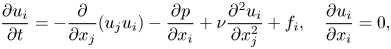
Here  $\langle \;\rangle$ denotes the ensemble averaging. In the prevalent local eddy diffusivity model, the turbulent scalar flux
  $\langle {u_i}\theta \rangle$ is approximated as
 \begin{equation} \langle {u_i}\theta \rangle ={-} {\kappa _{Tij}}\frac{{\partial \varTheta}}{{\partial {x_j}}} , \end{equation}
where  ${\kappa _{Tij}}$ is the eddy diffusivity tensor and the summation convention is used for repeated indices. The isotropic eddy diffusivity model is often assumed to be
 \begin{equation} \langle {u_i}\theta \rangle ={-} {\kappa _T}\frac{{\partial \varTheta}}{{\partial {x_i}}} , \end{equation}
where  ${\kappa _T} ( = {\kappa _{Tii}}/3 )$ is the eddy diffusivity. The eddy diffusivity model is local in space and time, in the sense that the scalar flux at a point and time is expressed in terms of physical quantities at the same point and time. This local approximation is only valid if the turbulence length and time scales are significantly smaller than the length and time scales of the mean-field variation (Corrsin Reference Corrsin1974). However, this condition does not always hold for actual turbulent flow.
A non-local expression for the scalar flux can be written as
 \begin{equation} \langle {u_i}\theta \rangle ({\boldsymbol{x}},t) ={-} \int \,{\mathrm{d}\kern0.06em {\boldsymbol{x'}}} \int_{ - \infty }^{t} \,{\mathrm{d}t'} {\kappa _{NLij}}({\boldsymbol{x}},t;{\boldsymbol{x'}},t')\frac{\partial }{{\partial {x'_j}}}\varTheta ({\boldsymbol{x'}},t') , \end{equation}
where  $\int \, {\mathrm {d}\kern0.7pt{\boldsymbol {x}}} = \int _{ - \infty }^{\infty } {\mathrm {d}\kern0.7pt x} \int _{ - \infty }^{\infty }\, {\mathrm {d} y} \int _{ - \infty }^{\infty }\, {\mathrm {d}z}$ (Hamba Reference Hamba1995, Reference Hamba2004). Here,
  ${\kappa _{NLij}}({\boldsymbol {x}},t;{\boldsymbol {x'}},t')$ is the non-local eddy diffusivity, representing the non-local effect of the mean scalar gradient at
  $({\boldsymbol {x'}},t')$ on the scalar flux at
  $({\boldsymbol {x}},t)$. Modifying the analysis by Kraichnan (Reference Kraichnan1964, Reference Kraichnan1987), Hamba (Reference Hamba1995) derived an expression for the non-local eddy diffusivity using Green's function as follows. The transport equation for scalar fluctuation is given by
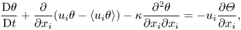 \begin{equation} \frac{{{\rm D}\theta }}{{{\rm D}t}} + \frac{\partial }{{\partial {x_i}}}({u_i}\theta - \langle {u_i}\theta \rangle ) - \kappa \frac{{{\partial ^{2}}\theta }}{{\partial {x_i}\partial {x_i}}} ={-} {u_i}\frac{{\partial \varTheta }}{{\partial {x_i}}} , \end{equation}
where  ${\rm D}/{\rm D}t = \partial /\partial t + {U_i}\partial /\partial {x_i}$ and
  $\kappa$ is the molecular diffusivity of the scalar. By considering the right-hand side of (2.6) as a source term for
  $\theta$, we introduce the Green's function
  ${g_i}({\boldsymbol {x}},t;{\boldsymbol {x'}},t')$ satisfying the following equation:
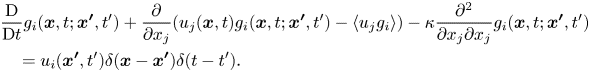 \begin{align} &\frac{{\rm D}}{{{\rm D}t}}{g_i}({\boldsymbol{x}},t;{\boldsymbol{x'}}, t') + \frac{\partial }{{\partial {x_j}}}({u_j}({\boldsymbol{x}}, t){g_i}({\boldsymbol{x}},t;{\boldsymbol{x'}},t') - \langle {u_j}{g_i}\rangle ) - \kappa \frac{{{\partial^{2}}}}{{\partial {x_j}\partial {x_j}}}{g_i}({\boldsymbol{x}},t;{\boldsymbol{x'}},t')\nonumber\\ &\quad = {u_i}({\boldsymbol{x'}},t')\delta ({\boldsymbol{x}} - {\boldsymbol{x'}})\delta (t - t') . \end{align}
Note that the velocity fluctuation  ${u_i}({\boldsymbol {x'}},t')$ is included on the right-hand side of (2.7). The Green's function
  ${g_i}({\boldsymbol {x}},t;{\boldsymbol {x'}},t')$ represents a scalar field at
  $({\boldsymbol x},t)$ associated with a point source at
  $({\boldsymbol x'},t')$ whose value is proportional to
  ${u_i}({\boldsymbol {x'}},t')$. Using Green's function, a formal solution of (2.6) can be written as
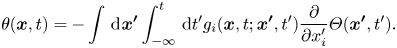 \begin{equation} \theta ({\boldsymbol{x}},t) ={-} \int\, {\mathrm{d}\kern0.06em {\boldsymbol{x'}}} \int_{ - \infty }^{t}\, {\mathrm{d}t'} {g_i}({\boldsymbol{x}},t;{\boldsymbol{x'}},t')\frac{\partial }{{\partial {x'_i}}}\varTheta ({\boldsymbol{x'}},t') . \end{equation}
Therefore, the scalar flux can be written as
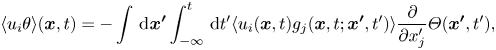 \begin{equation} \langle {u_i}\theta \rangle ({\boldsymbol{x}},t) ={-} \int\, {\mathrm{d}\kern0.06em {\boldsymbol{x'}}} \int_{ - \infty }^{t}\, {\mathrm{d}t'} \langle {u_i}({\boldsymbol{x}},t){g_j}({\boldsymbol{x}},t;{\boldsymbol{x'}},t')\rangle \frac{\partial }{{\partial {x'_j}}}\varTheta ({\boldsymbol{x'}},t') , \end{equation}
which yields
 \begin{equation} {\kappa _{NLij}}({\boldsymbol{x}},t;{\boldsymbol{x'}},t') = \langle {u_i}({\boldsymbol{x}},t){g_j}({\boldsymbol{x}},t; {\boldsymbol{x'}},t')\rangle . \end{equation}
Hamba (Reference Hamba2004) evaluated Green's function using the DNS data of turbulent channel flow to verify the non-local expression given by (2.9).
Let us consider the relationship between the non-local expression and local approximation. The non-local eddy diffusivity  ${\kappa _{NLij}}({\boldsymbol {x}},t;{\boldsymbol {x'}},t')$ has a non-zero value if the distance
  $|{\boldsymbol {x}} - {\boldsymbol {x'}}|$ and time difference
  $t - t'$ are comparable to or less than the turbulence length and time scales, respectively. If the mean scalar gradient
  $\partial \varTheta /\partial {x'_i}$ is nearly constant in this region in terms of scale and time, then the scalar flux can be approximated as
 \begin{equation} \langle {u_i}\theta \rangle ({\boldsymbol{x}},t) \simeq{-} {\kappa_{Lij}} ({\boldsymbol{x}},t) \frac{{\partial \varTheta }}{{\partial {x_j}}}, \end{equation}
where  ${\kappa _{Lij}} ({\boldsymbol {x}},t)$ is the local eddy diffusivity defined as
 \begin{equation} {\kappa _{Lij}}({\boldsymbol{x}},t) = \int\, {\mathrm{d}\kern0.06em {\boldsymbol{x'}}} \int_{ - \infty }^{t}\, {\mathrm{d}t'} {\kappa_{NLij}} ({\boldsymbol{x}},t;{\boldsymbol{x'}},t') . \end{equation}
Conversely, if the mean scalar gradient changes appreciably in the region, the local approximation is invalid and the non-local expression should be used to predict the scalar flux.
To apply the eddy diffusivity approximation given by (2.4) to turbulence simulations, we must further model the eddy diffusivity itself. In the  $K$–
$K$– $\varepsilon$ model, the local eddy diffusivity
  ${\kappa _T}$ in (2.4) is expressed as
 \begin{equation} {\kappa_T} = {C_\kappa}\frac{{{K^{2}}}}{\varepsilon} , \end{equation}
where  $K( = \langle u_i^{2}\rangle /2)$ denotes the turbulent kinetic energy,
  $\varepsilon [ = \nu \langle {(\partial {u_i}/\partial {x_j})^{2}}\rangle ]$ denotes its dissipation rate,
  $\nu$ denotes the molecular viscosity and
  ${C_\kappa }$ denotes a model constant with a typical value of 0.1. This expression can be empirically obtained using dimensional analysis and is proportional to the product of the turbulence intensity
  $K^{1/2}$ and the turbulence length scale
  $K^{3/2}/\varepsilon$. Moreover, it can be derived theoretically using the TSDIA as follows (Yoshizawa Reference Yoshizawa1998). Starting from the basic equations for velocity and a scalar quantity, and applying theoretical procedures to the scalar flux, an expression for the eddy diffusivity is obtained as
 \begin{equation} {\kappa _T} = \frac{1}{3}\int\, {\mathrm{d}{\boldsymbol{k}}} \int_{ - \infty }^{t}\, {\mathrm{d}t'} {G_\theta} ({\boldsymbol{k}},t,t'){Q_{ii}}({\boldsymbol{k}},t,t') , \end{equation}
where  $\int \, {\mathrm {d}{\boldsymbol {k}}} = \int _{ - \infty }^{\infty }\, {\mathrm {d}{k_x}} \int _{ - \infty }^{\infty }\, {\mathrm {d}{k_y}} \int _{ - \infty }^{\infty }\, {\mathrm {d}{k_z}}$. Here,
  ${Q_{ii}}({\boldsymbol {k}},t,t')$ and
  ${G_\theta }({\boldsymbol {k}},t,t')$ are the two-time velocity correlation and the mean Green's function for scalar fluctuation, respectively, expressed in wavenumber space. Because it is very difficult to evaluate
  ${Q_{ii}}({\boldsymbol {k}},t,t')$ and
  ${G_\theta }({\boldsymbol {k}},t,t')$ by solving their transport equations for inhomogeneous turbulence, their profiles were further assumed to be
 \begin{gather} {Q_{ij}}({\boldsymbol{k}},t,t') = {D_{ij}}({\boldsymbol{k}})E(k)\exp [ - \omega (k)|t - t'|] , \end{gather}
 \begin{gather}{G_\theta }({\boldsymbol{k}},t,t') = \exp [ - {\omega _\theta }(k)(t - t')] , \end{gather}
where  ${D_{ij}}({\boldsymbol {k}}) = {\delta _{ij}} - {k_i}{k_j}/{k^{2}}$,
  $E(k)$ is the energy spectrum and
  $\omega (k)$ and
  ${\omega _\theta }(k)$ are the inverse of the time scale for the velocity and scalar, respectively. The Kolmogorov spectrum and time scales were adopted for
  $E(k)$,
  $\omega (k)$ and
  ${\omega _\theta }(k)$ as
 \begin{gather} E(k) = \left\{ \begin{array}{@{}ll} {{C_K}{\varepsilon ^{2/3}}{k^{ - 5/3}}}, & {k \ge {k_c}}, \\ 0, & {k < {k_c}}, \end{array} \right. \end{gather}
 \begin{gather}\omega (k) = {C_\omega }{\varepsilon ^{1/3}}{k^{2/3}} , \end{gather}
 \begin{gather}{\omega _\theta }(k) = {C_{\omega \theta }}{\varepsilon^{1/3}}{k^{2/3}}, \end{gather}
where  ${k_c}[ = {(3{C_K}/2)^{3/2}}{K^{ - 3/2}}\varepsilon ]$ is the cutoff wavenumber in the energy-containing range and the model constants are given by
  ${C_K} = 1.5$,
  ${C_\omega } = 0.42$ and
  ${C_{\omega \theta }} = 1.6{C_\omega }$. Finally, substituting (2.15)–(2.19) into (2.14) and performing the integrals in (2.14) yields (2.13), with
  ${C_\kappa } = 0.136$. Therefore, the eddy diffusivity given by (2.13) reflects the behaviour of the two-time velocity correlation and the Green's function.
In contrast to the local eddy diffusivity, the model expression for the non-local eddy diffusivity appearing in (2.5) has not been studied extensively. When applying the non-local expression to turbulent channel flow, a one-dimensional spatially non-local expression was proposed as
 \begin{equation} {\kappa_{NLyy}}(y;y') \propto \langle u_y^{2}\rangle \exp ( - |y - y'|/L) , \end{equation}
where  $L$ is the turbulence length scale (Hamba Reference Hamba2004). This profile was obtained empirically and does not have a solid theoretical basis. In § 4 we systematically investigate the non-local eddy diffusivity in a manner similar to the TSDIA for the local eddy diffusivity described above.
3. The DNS of isotropic turbulence with inhomogeneous scalar
To verify the non-local expression given by (2.5), Hamba (Reference Hamba2004) examined the DNS data of a turbulent channel flow. However, the non-local eddy diffusivity showed a complex profile because of the anisotropy and inhomogeneity of the turbulence. It was difficult to propose a model expression for the non-local eddy diffusivity that agrees with such a complex profile. In this study, we examine the DNS data of homogeneous isotropic turbulence with an inhomogeneous mean scalar to systematically investigate the non-local eddy diffusivity. Because the non-local eddy diffusivity is determined solely by the velocity fluctuation, regardless of the mean scalar field, the profile of the non-local eddy diffusivity is isotropic and appropriate for an examination in a first step.
The DNS was performed as follows. Using a pseudo-spectral method, numerical solutions for the velocity were obtained from the Navier–Stokes and continuity equations
 \begin{equation} \frac{{\partial {u_i}}}{{\partial t}} ={-} \frac{\partial }{{\partial {x_j}}}({u_j}{u_i}) - \frac{{\partial p}}{{\partial {x_i}}} + \nu \frac{{{\partial ^{2}}{u_i}}}{{\partial x_j^{2}}} + {f_i} , \quad \frac{{\partial {u_i}}}{{\partial {x_i}}} = 0 , \end{equation}
where  $p$ is the pressure and
  $f_{i}$ is the external force. The mean velocity
  $U_{i}$ was set to zero. The size of the computational domain was
  $L_{x} \times L_{y} \times L_{z} = 2{\rm \pi} \times 2{\rm \pi} \times 2{\rm \pi}$ and the number of grid points was
  ${512^{3}}$. The velocity was normalised such that the initial velocity variance
  $\langle u_i^{2}\rangle$ was equal to unity. Hereafter, the physical quantities were non-dimensionalised by the initial turbulence intensity
  $\langle u_i^{2}\rangle ^{1/2}$ and the length scale
  $L_{x}/(2{\rm \pi} )$. The initial velocity spectrum was set to
  $E(k) \propto {k^{4}}\exp [ - 2{(k/{k_0})^{2}}]$, where
  ${k_0} = 3.5$. The external forcing of negative viscosity (Jiménez et al. Reference Jiménez, Wray, Saffman and Rogallo1993; Yamazaki, Ishihara & Kaneda Reference Yamazaki, Ishihara and Kaneda2002) was applied to low wavenumbers to maintain constant turbulent kinetic energy over time. The viscosity was set to
  $\nu = 6 \times {10^{ - 4}}$ and the Taylor micro-scale Reynolds number
  ${R_\lambda }( = {\langle u_x^{2}\rangle ^{1/2}}\lambda /\nu )$ was 122.
In addition to the velocity field, we solved the equation for scalar fluctuation
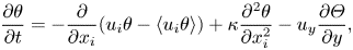 \begin{equation} \frac{{\partial \theta }}{{\partial t}} ={-} \frac{\partial }{{\partial {x_i}}}({u_i}\theta - \langle {u_i}\theta \rangle ) + \kappa \frac{{{\partial ^{2}}\theta }}{{\partial x_i^{2}}} - {u_y}\frac{{\partial \varTheta }}{{\partial y}} , \end{equation}
where  $\kappa$ was equal to
  $\nu$. Here, a fixed one-dimensional profile of the mean scalar
  $\varTheta (y)$ was used such that the scalar fluctuation was inhomogeneous in the
  $y$ direction and homogeneous in the
  $x$ and
  $z$ directions. We adopted the four functions of the mean scalar gradient listed in table 1 and their profiles are shown in figure 1. The cosine function was used as a simple profile of an inhomogeneous mean scalar. The length scale of the mean scalar field in case 2 was half that of case 1. The length scale in cases 3 and 4 was the same as that in cases 1 and 2, respectively, but in cases 3 and 4 the magnitude of the positive peak was greater than that of the negative peak.
Table 1. The functions of mean scalar gradient  $\partial \varTheta / \partial y$ for the four cases.
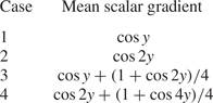
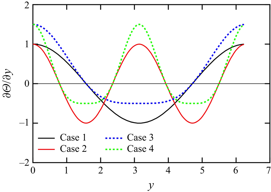
Figure 1. Profiles of the mean scalar gradient  $\partial \varTheta /\partial y$ as functions of
  $y$ for the four cases.
Because the velocity field is statistically steady and homogeneous in the  $x$ and
  $z$ directions, the non-local expression given by (2.5) can be rewritten as
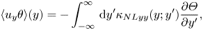 \begin{equation} \langle {u_y}\theta \rangle (y) ={-} \int_{ - \infty }^{\infty}\, {\mathrm{d} y'} {\kappa _{NLyy}}(y;y')\frac{{\partial \varTheta }}{{\partial y'}}, \end{equation}
where
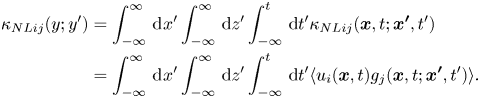 \begin{align} {\kappa _{NLij}}(y;y') &= \int_{ - \infty }^{\infty}\, {\mathrm{d}\kern0.06em x'} \int_{ - \infty }^{\infty}\, {\mathrm{d}z'} \int_{ - \infty }^{t}\, {\mathrm{d}t'} {\kappa _{NLij}}({\boldsymbol{x}},t;{\boldsymbol{x'}},t')\nonumber\\ &= \int_{ - \infty }^{\infty}\, {\mathrm{d}\kern0.06em x'} \int_{ - \infty }^{\infty}\, {\mathrm{d}z'} \int_{ - \infty }^{t}\, {\mathrm{d}t'} \langle {u_i}({\boldsymbol{x}},t){g_j}({\boldsymbol{x}},t;{\boldsymbol{x'}},t') \rangle . \end{align}
The non-local eddy diffusivity  ${\kappa _{NLyy}}$ appearing in (3.3) is a function of
  $y$ and
  $y'$ only. To evaluate it, we must calculate the integrals with respect to
  $x'$,
$x'$,  $z'$ and
  $t'$ in (3.4); it would incur considerable computational costs. To reduce computational costs, we introduce another Green's function
  ${g_i}({\boldsymbol {x}},t;y')$ defined as
 \begin{equation} {g_i}({\boldsymbol{x}},t;y') = \int_{ - \infty }^{\infty}\, {\mathrm{d}\kern0.06em x'} \int_{ - \infty }^{\infty}\, {\mathrm{d}z'} \int_{ - \infty }^{t}\, {\mathrm{d}t'} {g_i}({\boldsymbol{x}},t;{\boldsymbol{x'}},t'), \end{equation}
which satisfies the following equation:
 \begin{align} &\frac{{\rm D}}{{{\rm D}t}}{g_i}({\boldsymbol{x}},t;y') + \frac{\partial }{{\partial {x_j}}}({u_j}({\boldsymbol{x}},t){g_i}({\boldsymbol{x}},t;y') - \langle {u_j}{g_i}\rangle ) - \kappa \frac{{{\partial ^{2}}}}{{\partial {x_j}\partial {x_j}}}{g_i}({\boldsymbol{x}},t;y') \nonumber\\ &\quad = {u_i}({\boldsymbol{x}},t)\delta (y - y') . \end{align}
In contrast to (2.7), only a delta function with respect to  $y-y'$ is included on the right-hand side of (3.6). The Green's function
  ${g_i}({\boldsymbol {x}},t;y')$ represents a scalar field at
  $({\boldsymbol x},t)$ associated with a statistically steady source on the
  $x$–
$x$– $z$ plane at
  $y=y'$ whose value is proportional to
  ${u_i}({\boldsymbol {x'}},t')$ at each point and time. We solved (3.6) instead of (2.7) to obtain the Green's function
  ${g_i}({\boldsymbol {x}},t;y')$. We can then evaluate the non-local eddy diffusivity as
 \begin{equation} {\kappa _{NLij}}(y;y') = \langle {u_i}({\boldsymbol{x}},t){g_j}({\boldsymbol{x}},t;y')\rangle , \end{equation}
without any additional integrals. Because the velocity field is also homogeneous in the  $y$ direction, the non-local eddy diffusivity
  ${\kappa _{NLij}}(y;y')$ is only a function of the separation
  $y - y'$, and the local eddy diffusivity, defined as
 \begin{equation} {\kappa _{Lij}}(y) = \int_{ - \infty }^{\infty}\, {\mathrm{d} y'} {\kappa _{NLij}}(y;y') , \end{equation}
is constant in  $y$. Consequently, the non-local and local expressions for the scalar flux can be written as follows:
 \begin{gather} {\langle {u_y}\theta \rangle _{NL}} ={-} \int_{ - \infty }^{\infty}\, {\mathrm{d} y'} {\kappa _{NLyy}}(y - y')\frac{{\partial \varTheta }}{{\partial y'}} , \end{gather}
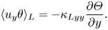 \begin{gather}{\langle {u_y}\theta \rangle _L} ={-} {\kappa _{Lyy}}\frac{{\partial \varTheta }}{{\partial y}} . \end{gather}
In the present DNS, the profiles of  ${\kappa _{NLyy}}(y - y')$ and
  $\langle {u_y}\theta \rangle$ and the value of
  ${\kappa _{Lyy}}( = 0.23)$ were obtained by averaging over the
  $x$–
$x$– $z$ plane and over a time period of 2.5 normalised by
  $L_{x}/(2{\rm \pi} \langle u_i^{2}\rangle ^{1/2})$.
Before examining the non-local effect, let us mention the value of the local eddy diffusivity  ${\kappa _{Lyy}} = 0.23$. Substituting
  ${\kappa _{Lyy}} = 0.23$,
  $K=0.50$ and
  $\varepsilon =0.19$ evaluated in the DNS into (2.13), we obtain
  ${C_\kappa } = 0.17$, which is relatively large compared with the standard value
  ${C_\kappa } = 0.1$ mentioned in § 2. This difference can be understood by considering the transport equation for
  $\langle {u_y}\theta \rangle$ as follows. The production term in the transport equation is
  $- \langle u_y^{2}\rangle \partial \varTheta /\partial y$ and the pressure–scalar-gradient term can be modelled as
 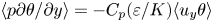 $\langle p \partial \theta /\partial y \rangle = - {C_p}(\varepsilon /K)\langle {u_y}\theta \rangle$, which represents the dissipation of
  $\langle {u_y}\theta \rangle$. By assuming a balance between the two terms, we can obtain the eddy diffusivity model
 \begin{equation} \langle {u_y}\theta \rangle ={-} \frac{K}{{{C_p}\varepsilon }}\langle u_y^{2}\rangle \frac{{\partial \varTheta }}{{\partial y}} , \end{equation}
which indicates that 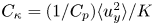 ${C_\kappa } = (1/{C_p})\langle u_y^{2}\rangle /K$. The ratio
  $\langle u_y^{2}\rangle /K$ is
  $2/3$ for homogeneous isotropic turbulence and is approximately
  $1/3$ for a turbulent shear flow such as a channel flow. Because the eddy diffusivity model is usually optimised for turbulent shear flow, the standard value of
  ${C_\kappa }$ is small compared with the present value obtained for homogeneous isotropic turbulence. A similar discussion on the model constant
  ${C_\mu }$ for eddy viscosity is given in Hanjalić & Launder (Reference Hanjalić and Launder2011).
Figure 2 shows the profiles of the non-local eddy diffusivity  ${\kappa _{NLyy}}(y - y')$ as functions of
  $(y - y')/L$. The separation
  $y-y'$ was normalised by the integral length scale
  $L( = \int _{0}^{\infty } \mathrm {d}r_{x} \langle u_{x}({\boldsymbol {x}},t) u_{x}({\boldsymbol {x}}+r_{x}{\boldsymbol {e}}_{x},t)\rangle / \langle u_{x}^{2}({\boldsymbol {x}},t) \rangle )$, which is equal to 0.465 in the present DNS. The black line represents the DNS value obtained from (3.7), whereas the other lines for models 1 and 2 are mentioned in § 4. As the profile is symmetric with respect to
  $(y - y')/L = 0$, it is plotted only in the positive region at
 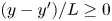 $(y - y')/L \geq 0$. It exhibits a sharp peak at
  $(y - y')/L = 0$ and decays quickly as
  $(y - y')/L$ increases. The value at
  $(y - y')/L = 1$ is 9 % of the peak value. This profile suggests that the value of
  $\partial \varTheta /\partial y'$ at
 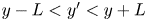 $y - L < y' < y + L$ mainly affects the scalar flux at
  $y$ in (3.9), and that we should include the non-local mean scalar profile within the integral length scale to accurately predict the scalar flux.
Figure 2. Profiles of the non-local eddy diffusivity  ${\kappa _{NLyy}}(y - y')$ as functions of
  $(y - y')/L$ for DNS and models 1 and 2. The separation
  $y - y'$ was normalised by the integral length scale
  $L ( = 0.465)$.
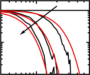
Figure 3 shows the profiles of the scalar fluxes as functions of  $y$ for the four cases. Here ‘DNS’ denotes
  $\langle {u_y}\theta \rangle$ evaluated directly, ‘Local’ denotes
  ${\langle {u_y}\theta \rangle _L}$ given by (3.10) and ‘Non-local’ denotes
  ${\langle {u_y}\theta \rangle _{NL}}$ given by (3.9). The profile of
  ${\langle {u_y}\theta \rangle _{Model}}$ given by (4.30) for model 2 is discussed in § 4. The profiles of
  ${\langle {u_y}\theta \rangle _{NL}}$ plotted as blue lines agree with the DNS values for all cases. This verifies the non-local expression for the scalar flux given by (3.3). In contrast, the profiles of
  ${\langle {u_y}\theta \rangle _L}$, plotted as red lines, overpredicted the DNS values. The profiles of
  ${\langle {u_y}\theta \rangle _L}$ were determined using the local value of
  $\partial \varTheta /\partial y$ with the constant
  ${\kappa _{Lyy}} = 0.23$. For example, the positive peak values in cases 1 and 2 shown in figures 3(a) and 3(b) are 0.23 because
  $\partial \varTheta /\partial y = - 1$ at the peak locations. However, the peak of the DNS values was less than 0.23. The small value can be accounted for by the non-local effect; the DNS value is small compared with the local model because the scalar flux at the peak is affected non-locally by
  $\partial \varTheta /\partial y$ at remote points where its magnitude is less than unity. This tendency was more significant in case 2 than in case 1 because the length scale of the mean scalar field was small in case 2.
Figure 3. Profiles of the scalar fluxes  $\langle {u_y}\theta \rangle$,
  ${\langle {u_y}\theta \rangle _L}$,
  ${\langle {u_y}\theta \rangle _{NL}}$ and
  ${\langle {u_y}\theta \rangle _{Model}}$ as functions of
  $y$ for (a) case 1, (b) case 2, (c) case 3 and (d) case 4. Insets show enlarged profiles near the first zero point.
In addition to the small peak values, another non-local effect appeared in cases 3 and 4. As clearly seen in the insets of figures 3(c) and 3(d), the locations of the zero points are different between the local model and the DNS value. For example, in case 3, shown in figure 3(c), the zero point of the local model is located at  $y = 1.57( = {\rm \pi}/2)$ where
  $\partial \varTheta /\partial y = 0$. However, the zero point of the DNS value shifts to
  $y = 1.67$. This difference in the zero point location indicates a phenomenon of the counter-gradient diffusion; that is, in the region at
  $1.57 < y < 1.67$, both the values of
  $\partial \varTheta /\partial y$ and
  $\langle {u_y}\theta \rangle$ are negative, which is inconsistent with the gradient diffusion approximation. This behaviour of the DNS value cannot be accounted for by the local eddy diffusivity model. This counter-gradient diffusion can be understood from a non-local point of view. Let us consider the scalar flux
  $\langle {u_y}\theta \rangle$ at
  $y = 1.62$. The magnitude of
  $\partial \varTheta /\partial y$ at
  $y < 1.57$ was greater than that of
  $\partial \varTheta /\partial y$ at
  $y > 1.57$, as indicated by the blue line in figure 1. The non-local contribution from the positive
  $\partial \varTheta /\partial y$ at
  $y < 1.57$ to
  $\langle {u_y}\theta \rangle$ at
  $y = 1.62$ is greater than the contribution from the negative
  $\partial \varTheta /\partial y$ at
  $y > 1.57$. Consequently,
  $\langle {u_y}\theta \rangle$ becomes negative at
  $y = 1.62$ even though
  $\partial \varTheta /\partial y$ is negative at
  $y = 1.62$. The counter-gradient diffusion was more significant in case 4 than in case 3 because the length scale of the mean scalar field was smaller in case 4. In summary, because of the non-local effect, the peak value of the scalar flux is less than the locally estimated value, and the counter-gradient diffusion appears near the zero point. These findings indicate the importance of the non-local expression for the scalar flux given by (3.3). The non-local modelling correctly describes counter-gradient diffusion that local models are not able to represent.
4. Modelling the non-local eddy diffusivity
In § 3 the non-local expression for the scalar flux given by (3.3) was assessed using the DNS data of homogeneous isotropic turbulence with an inhomogeneous mean scalar. The profile of the non-local eddy diffusivity  ${\kappa _{NLyy}}(y - y')$ was shown in figure 2. In this section we further analyse the non-local eddy diffusivity and systematically propose its model expression. In § 3 we treated one-dimensional profiles of the mean scalar
  $\varTheta (y)$ and considered the following non-local eddy diffusivity:
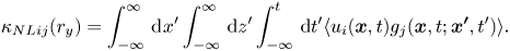 \begin{equation} {\kappa _{NLij}}({r_y}) = \int_{ - \infty }^{\infty}\, {\mathrm{d}\kern0.06em x'} \int_{ - \infty }^{\infty}\, {\mathrm{d}z'} \int_{ - \infty }^{t}\, {\mathrm{d}t'} \langle {u_i}({\boldsymbol{x}},t){g_j}({\boldsymbol{x}}, t;{\boldsymbol{x'}},t')\rangle . \end{equation}
Here, integrals are performed with respect to  $x'$,
$x'$,  $z'$ and
  $t'$, and the non-local eddy diffusivity becomes a one-dimensional function of
  ${r_y}( = y - y')$. However, in the case of general profiles of the mean scalar varying in three directions, we must consider the original expression for the non-local eddy diffusivity for steady turbulence
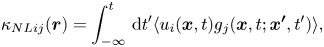 \begin{equation} {\kappa _{NLij}}({\boldsymbol{r}}) = \int_{ - \infty }^{t}\, {\mathrm{d}t'} \langle {u_i}({\boldsymbol{x}},t){g_j}({\boldsymbol{x}},t; {\boldsymbol{x'}},t')\rangle , \end{equation}
which is a three-dimensional function of  ${\boldsymbol {r}}( = {\boldsymbol {x}} - {\boldsymbol {x'}})$. Because the turbulent velocity field is isotropic and the Green's function is determined solely by the velocity fluctuation, the non-local eddy diffusivity can be expressed in the following isotropic form of a second-rank tensor:
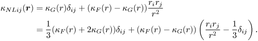 \begin{align} {\kappa _{NLij}}({\boldsymbol{r}}) &= {\kappa _G}(r){\delta _{ij}} + ({\kappa _F}(r) - {\kappa _G}(r))\frac{{{r_i}{r_j}}}{{{r^{2}}}}\nonumber\\ &= \frac{1}{3}({\kappa _F}(r) + 2{\kappa _G}(r)){\delta _{ij}} + ({\kappa _F}(r) - {\kappa _G}(r))\left( {\frac{{{r_i}{r_j}}}{{{r^{2}}}} - \frac{1}{3}{\delta _{ij}}} \right). \end{align}
Here  ${\kappa _F}(r)$ and
  ${\kappa _G}(r)$ are functions of
  $r(=|{\boldsymbol r}|)$ and correspond to the longitudinal and lateral correlations, respectively. Note that the second line of (4.3) consists of two parts: the spherically symmetric part and the deviatoric traceless part. It was difficult to evaluate
  ${\kappa _F}(r)$ and
  ${\kappa _G}(r)$ separately using the present DNS data. In this study, we restrict ourselves to the spherically symmetric part of the non-local eddy diffusivity, and assume that
 \begin{equation} {\kappa _{NLij}}({\boldsymbol{r}}) = \kappa_{NL}(r)\delta_{ij}, \end{equation}
where
 \begin{equation} {\kappa _{NL}}(r) \equiv \tfrac{1}{3}{\kappa _{NLii}}({\boldsymbol{r}}) = \tfrac{1}{3}({\kappa _F}(r) + 2{\kappa _G}(r)) . \end{equation}
This can be further written as the time integral
 \begin{equation} {\kappa _{NL}}(r) = \int_0^{\infty}\, {\mathrm{d}\tau } {\kappa _{NL}}(r,\tau ) , \end{equation}
where
 \begin{equation} {\kappa _{NL}}(r,\tau ) = \tfrac{1}{3}{\kappa _{NLii}}({\boldsymbol{r}},\tau ) = \tfrac{1}{3}\langle {u_i}({\boldsymbol{x}},t){g_i}({\boldsymbol{x}},t; {\boldsymbol{x'}},t')\rangle, \end{equation}
and  $\tau = t - t'$. Using the DNS data of homogeneous isotropic turbulence described in § 3, we evaluate the profile of the non-local eddy diffusivity. Because it incurs considerable computational costs to directly evaluate (4.2) and (4.7), we first obtain the profiles of
  ${\kappa _{NL}}({r_y})$ and
  ${\kappa _{NL}}({r_y},\tau )$ as functions of
  ${r_y}$, and then transform them into
  ${\kappa _{NL}}(r)$ and
  ${\kappa _{NL}}(r,\tau )$, respectively (see Appendix A for details). The profile of
  $\kappa _{NL}(r_{y})$ was obtained by averaging over the
  $x$–
$x$– $z$ plane and over a time period of 15 normalised by
  $L_{x}/(2{\rm \pi} \langle u_i^{2}\rangle ^{1/2})$, and the profile of
  $\kappa _{NL}(r_{y},\tau )$ was obtained by averaging over the
  $x$–
$x$– $z$ plane and over 40 samples.
Figure 4 shows the profiles of  ${r^{2}}{\kappa _{NL}}(r)$ as functions of
  $r/L$. The black line represents the DNS value, whereas the other lines for models 1 and 2 are mentioned later. Because the profile of
  ${\kappa _{NL}}(r)$ has a sharp peak at
  $r = 0$ and decays rapidly as
  $r$ increases, it was multiplied by a factor of
  ${r^{2}}$ to clearly show its profile. The profile of
  ${r^{2}}{\kappa _{NL}}(r)$ exhibits a peak at
  $r = 0.03$ and decreases gradually as
  $r$ increases. In (4.6),
  ${\kappa _{NL}}(r)$ is written as the time integral of
  ${\kappa _{NL}}(r,\tau )$. Figure 5 shows the profiles of
  ${\kappa _{NL}}(r,\tau )$ as functions of
  $r/L$ at
  $\tau = 0.2$, 0.4 and 0.6. The turbulence time scale
  $T( = K/\varepsilon )$ is 2.7 in the present DNS. Considering the initial condition
  ${g_i}({\boldsymbol {x}},t';{\boldsymbol {x'}},t') = {u_i}({\boldsymbol {x'}},t')\delta ({\boldsymbol {x}} - {\boldsymbol {x'}})$, the profile at
  $\tau =0$ is given by
 \begin{equation} {\kappa _{NL}}(r,0) = \tfrac{1}{3}\langle {u_i}({\boldsymbol{x}},t){g_i}({\boldsymbol{x}},t;{\boldsymbol{x'}},t)\rangle = \tfrac{1}{3}\langle u_i^{2}({\boldsymbol{x}},t)\rangle \delta ({\boldsymbol{x}} - {\boldsymbol{x'}}) , \end{equation}
which is proportional to a delta function. Figures 5(a)–5(c) indicate that the peak value of  ${\kappa _{NL}}(r,\tau )$ decays rapidly as
  $\tau$ increases, although the normalised time
  $\tau /T$ is less than 0.3. However, the width of the profile gradually increased as
  $\tau$ increased. This means that the spatial region in which the mean scalar gradient non-locally affects the scalar flux is very narrow for small
  $\tau$ and becomes wider as
  $\tau$ increases.
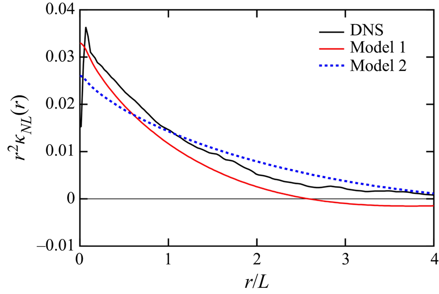
Figure 4. Profiles of  ${r^{2}}{\kappa _{NL}}(r)$ as functions of
  $r/L$ for DNS and models 1 and 2.
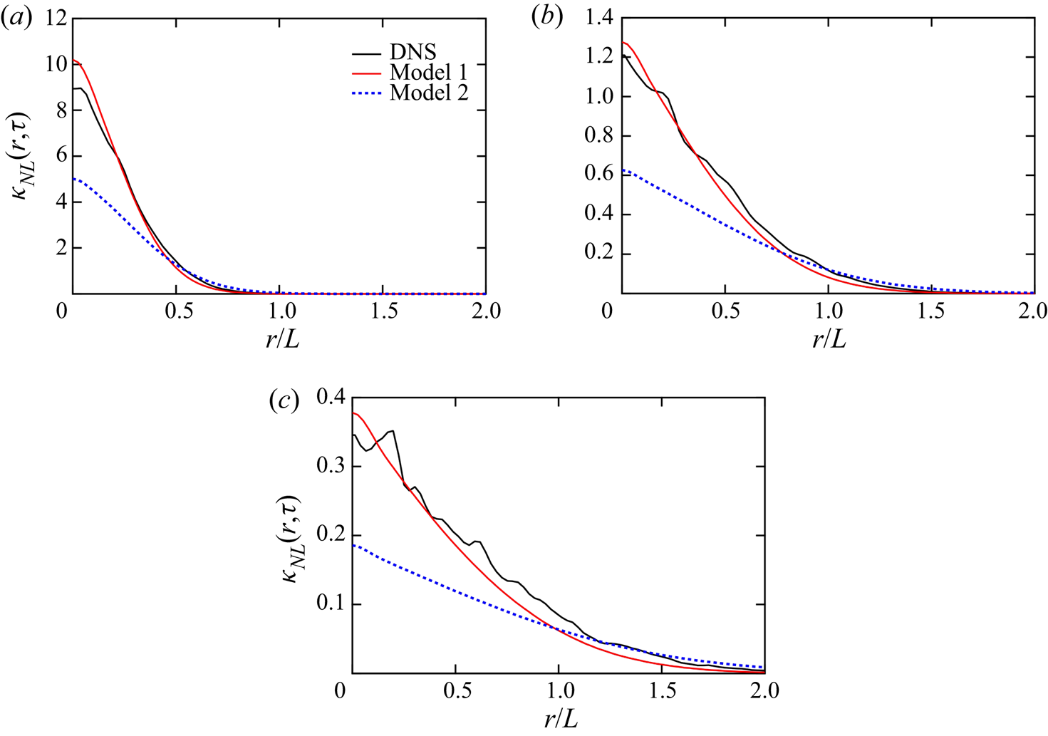
Figure 5. Profiles of  ${\kappa _{NL}}(r,\tau )$ as functions of
  $r/L$ for DNS and models 1 and 2 at (a)
  $\tau = 0.2$, (b)
  $\tau = 0.4$ and (c)
  $\tau = 0.6$.
Next, we investigate the profiles of  ${\kappa _{NL}}(r)$ and
  ${\kappa _{NL}}(r,\tau )$ from a physical point of view and propose a model expression in a manner similar to that of DIA and TSDIA. By replacing
  ${u_i}({\boldsymbol {x'}},t')$ with unity on the right-hand side of (2.7), we can obtain the transport equation for the ordinary Green's function
  $g({\boldsymbol {x}},t;{\boldsymbol {x'}},t')$ for scalar fluctuation. Here, we assume the following relationship:
 \begin{equation} {g_i}({\boldsymbol{x}},t;{\boldsymbol{x'}},t') = g({\boldsymbol{x}},t;{\boldsymbol{x'}},t'){u_i}({\boldsymbol{x'}},t') . \end{equation}
The non-local eddy diffusivity can then be written as
 \begin{equation} {\kappa _{NLij}}({\boldsymbol{x}},t;{\boldsymbol{x'}},t') = \langle {u_i}({\boldsymbol{x}},t)g({\boldsymbol{x}},t;{\boldsymbol{x'}},t') {u_j}({\boldsymbol{x'}},t')\rangle. \end{equation}
A similar expression for eddy diffusivity was theoretically derived in the DIA by Kraichnan (Reference Kraichnan1964, Reference Kraichnan1987). By factoring (4.10) into the products of two averages in a manner similar to the DIA, we obtain the approximation
 \begin{equation} {\kappa _{NLij}}({\boldsymbol{r}},\tau ) = G({\boldsymbol{r}},\tau ){Q_{ij}}({\boldsymbol{r}},\tau ), \end{equation}
where  ${Q_{ij}}({\boldsymbol {r}},\tau )( = \langle {u_i}({\boldsymbol {x}},t){u_j}({\boldsymbol {x'}},t')\rangle )$ denotes the two-point, two-time velocity correlation. Here,
  $G({\boldsymbol {r}},\tau )$ can simply be a proportional coefficient between
  ${\kappa _{NLij}}({\boldsymbol {r}},\tau )$ and
  ${Q_{ij}}({\boldsymbol {r}},\tau )$ and does not have to be identical to the mean Green's function
  $\langle g({\boldsymbol {x}},t;{\boldsymbol {x'}},t')\rangle$ (Hamba Reference Hamba2005). Nevertheless, we expect that
  $G({\boldsymbol {r}},\tau )$ will behave like a mean Green's function. Using (4.11) we can calculate the local eddy diffusivity
  ${\kappa _L}$ as follows:
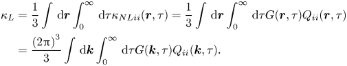 \begin{align} {\kappa _L} &= \frac{1}{3}\int\, {\mathrm{d}{\boldsymbol{r}}} \int_0^{\infty}\, {\mathrm{d}\tau } {\kappa _{NLii}}({\boldsymbol{r}},\tau ) = \frac{1}{3}\int\, {\mathrm{d}{\boldsymbol{r}}} \int_0^{\infty}\, {\mathrm{d}\tau } G({\boldsymbol{r}},\tau ){Q_{ii}} ({\boldsymbol{r}},\tau)\nonumber\\ &= \frac{{{{(2{\rm \pi} )}^{3}}}}{3}\int\, {\mathrm{d}{\boldsymbol{k}}} \int_0^{\infty}\, {\mathrm{d}\tau } G({\boldsymbol{k}},\tau ){Q_{ii}}({\boldsymbol{k}},\tau ) . \end{align}
This expression is the same as (2.14), except for a factor of  ${(2{\rm \pi} )^{3}}$, which indicates that (4.11) is consistent with the TSDIA. The difference in the factor of
  ${(2{\rm \pi} )^{3}}$ is simply due to the difference in the definition of the Fourier transform.
First, we examine the behaviour of the velocity correlation  ${Q_{ii}}({\boldsymbol {r}},\tau )$ appearing in (4.11). Figure 6 shows the profiles of
  ${Q_{ii}}(r,\tau )$ as functions of
  $r/L$ at
  $\tau = 0$, 0.2, 0.4 and 0.6. The peak value at
  $r = 0$ decreased gradually as
  $\tau$ increased, whereas the profile at
  $r/L>1.2$ hardly changed. We examined this decay in wavenumber space. Following (2.15) assumed in the TSDIA, the Fourier coefficient
  ${Q_{ij}}({\boldsymbol {k}},\tau )[ = {(2{\rm \pi} )^{ - 3}}\int \, {\mathrm {d}{\boldsymbol {r}}} {Q_{ij}}({\boldsymbol {r}},\tau )\exp ( - \mathrm {i}{\boldsymbol {k}} \boldsymbol {\cdot } {\boldsymbol {r}})]$ is expressed as
 \begin{equation} {Q_{ij}}({\boldsymbol{k}},\tau ) = {(2{\rm \pi} )^{3}}{Q_{ij}}({\boldsymbol{k}}){G_Q}({\boldsymbol{k}},\tau ) , \end{equation}
where  ${Q_{ij}}({\boldsymbol {k}}) = {Q_{ij}}({\boldsymbol {k}},0)$. The time-dependent part
  ${G_Q}({\boldsymbol {k}},\tau )$ represents the decay of the two-time velocity correlation with an increasing time difference. Figure 7(a) shows the profiles of
  ${Q_{ii}}(k,\tau )/2$ as functions of
  $k(=|{\boldsymbol k}|)$ at
  $\tau = 0$, 0.2, 0.4 and 0.6. The high-wavenumber part decays quickly as
  $\tau$ increases, whereas the low-wavenumber part decreases slightly. We examined this behaviour by normalising it with the initial profile
  ${Q_{ii}}(k,0)$, as shown in figure 7(b). The normalised value corresponds to the time-dependent part
  ${G_Q}(k,\tau )$ as
 \begin{equation} {Q_{ii}}({\boldsymbol{k}},\tau)/{Q_{ii}}({\boldsymbol{k}},0) = {(2{\rm \pi} )^{3}}{G_Q}(k,\tau). \end{equation}
In this study we assume the following function for  ${G_Q}(k,\tau )$:
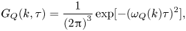 \begin{gather} {G_Q}(k,\tau ) = \frac{1}{{{{(2{\rm \pi} )}^{3}}}}\exp [ - {({\omega _Q}(k)\tau )^{2}}] , \end{gather}
 \begin{gather}{\omega _Q}(k) = {C_{\omega Q}}{u_0}k. \end{gather}
Here 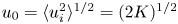 ${u_0} = {\langle u_i^{2}\rangle ^{1/2}} = {(2K)^{1/2}}$ and
  ${C_{\omega Q}} = 0.25$. The corresponding profiles of
  ${Q_{ii}}({\boldsymbol {k}},\tau )/ {Q_{ii}}({\boldsymbol {k}},0)$ are plotted as red dotted lines in figure 7(b), and agree fairly well with the DNS values. The inverse of time
  ${\omega _Q}(k)$, given by (4.16), is proportional to
  $k$. This dependence on
  $k$ is reasonable because the identical behaviour for the Eulerian two-time velocity correlation has been discussed and numerically evaluated (Tennekes & Lumley Reference Tennekes and Lumley1972; Matsumoto et al. Reference Matsumoto, Otsuki, Ooshida and Goto2021). The same profile of the velocity correlation as in (4.15) was also investigated by considering a simple problem in which large-scale eddies convect small-scale eddies without distorting them (Kraichnan Reference Kraichnan1964; Yoshizawa Reference Yoshizawa1998).
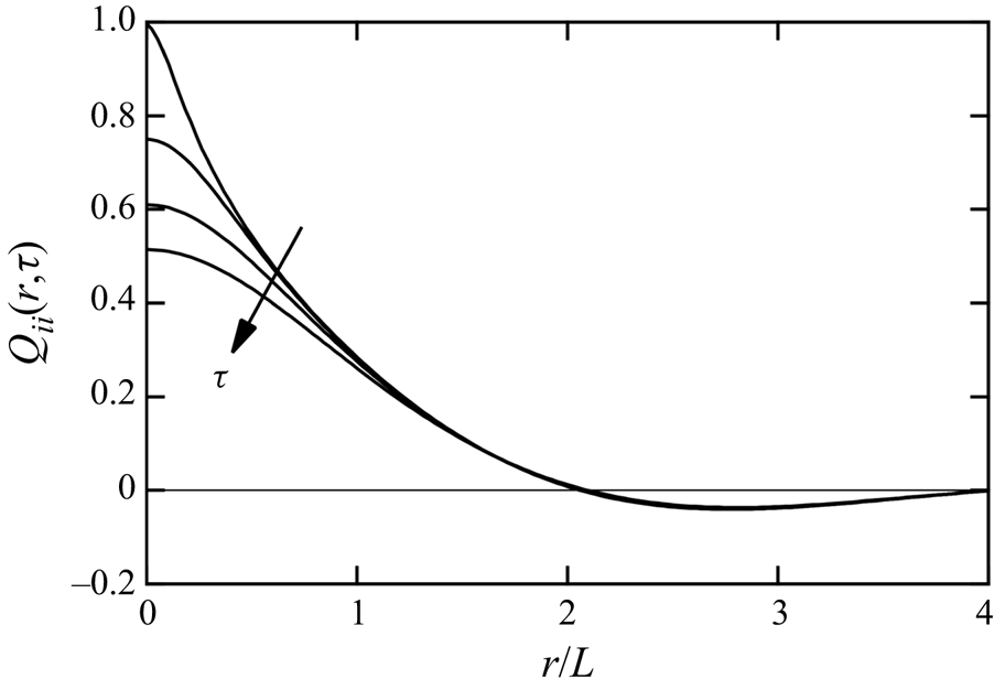
Figure 6. Profiles of  ${Q_{ii}}(r,\tau )$ as functions of
  $r/L$ at
  $\tau = 0$, 0.2, 0.4 and 0.6.
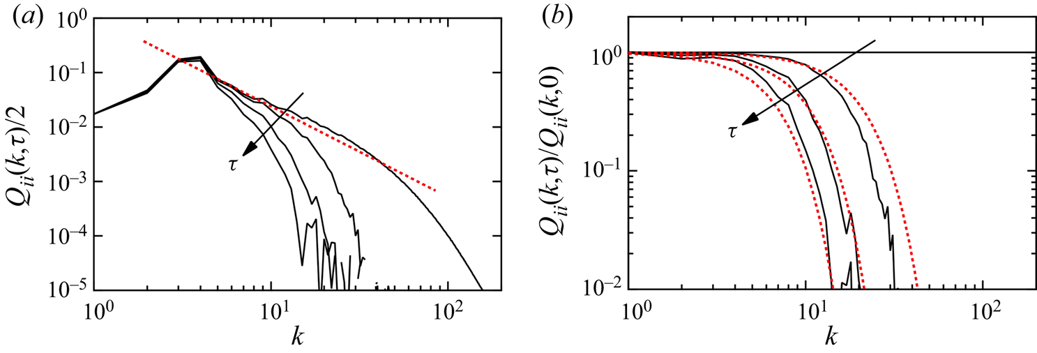
Figure 7. Profiles of  ${Q_{ii}}(k,\tau )$ as functions of
  $k$ at
  $\tau = 0$, 0.2, 0.4 and 0.6: (a)
  ${Q_{ii}}(k,\tau )/2$ and (b)
  ${Q_{ii}}(k,\tau )/{Q_{ii}}(k,0)$. The red dotted line in (a) represents the Kolmogorov spectrum given by (4.28) for
  ${C_K} = 1.7$. The red dotted lines in (b) represent
  ${(2{\rm \pi} )^{3}}{G_Q}(k,\tau )$ given by (4.15).
Next, we examine the non-local eddy diffusivity  ${\kappa _{NLij}}({\boldsymbol {r}},\tau )$ given by (4.11). The velocity correlation given by (4.13) can be written in physical space as
 \begin{equation} {Q_{ij}}({\boldsymbol{r}},\tau ) = \int\, {\mathrm{d}{\boldsymbol{r'}}} {G_Q}({\boldsymbol{r}} - {\boldsymbol{r'}},\tau ){Q_{ij}}({\boldsymbol{r'}}) , \end{equation}
where  ${Q_{ij}}({\boldsymbol {r}}) = {Q_{ij}}({\boldsymbol {r}},0)$. Substituting (4.17) into (4.11), we obtain
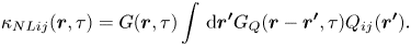 \begin{equation} {\kappa _{NLij}}({\boldsymbol{r}},\tau ) = G({\boldsymbol{r}},\tau )\int\, {\mathrm{d}{\boldsymbol{r'}}} {G_Q}({\boldsymbol{r}} - {\boldsymbol{r'}},\tau ){Q_{ij}}({\boldsymbol{r'}}) . \end{equation}
This expression is considerably complex; substituting it into (2.5), we obtain a non-local expression for the scalar flux containing double spatial integrals. By comparing figures 5 and 6, we can see that  $G({\boldsymbol {r}},\tau )$ decays rapidly, whereas
  ${Q_{ii}}({\boldsymbol {r}},\tau )$ decreases slowly. In this study, by neglecting the time-dependent part of
  ${Q_{ii}}({\boldsymbol {r}},\tau )$, we assume the following simple expression:
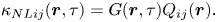 \begin{equation} {\kappa _{NLij}}({\boldsymbol{r}},\tau ) = G({\boldsymbol{r}},\tau ){Q_{ij}}({\boldsymbol{r}}) . \end{equation}
Thereby, the non-local eddy diffusivity can be written as
 \begin{gather} {\kappa _{NL}}(r,\tau ) = \tfrac{1}{3}G(r,\tau ){Q_{ii}}({\boldsymbol{r}}) , \end{gather}
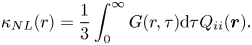 \begin{gather}{\kappa _{NL}}(r) = \frac{1}{3}\int_0^{\infty} {G(r,\tau )\mathrm{d}\tau } {Q_{ii}}({\boldsymbol{r}}) . \end{gather}
Moreover, the non-local eddy diffusivity given by (3.4), discussed in § 3, can be written as
 \begin{equation} {\kappa _{NLyy}}(y - y') = \int_{ - \infty }^{\infty}\, {\mathrm{d}{r_x}} \int_{ - \infty }^{\infty}\, {\mathrm{d}{r_z}} {\kappa _{NL}}(r) , \end{equation}
where (4.4) is assumed.
Similar to the discussion in (2.14)–(2.19) for the TSDIA, we further investigate the functions  $G(r,\tau )$ and
  ${Q_{ii}}({\boldsymbol {r}})$ to construct a model expression for the non-local eddy diffusivity. In (2.15) and (2.16) the time-dependent parts are given by the same exponential function except for the model constant. We also assume the same function between
  ${G_Q}(k,\tau )$ given by (4.15) and
  $G(k,\tau )$ as follows:
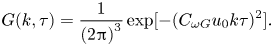 \begin{equation} G(k,\tau ) = \frac{1}{{{{(2{\rm \pi} )}^{3}}}}\exp [ - {({C_{\omega G}}{u_0}k\tau )^{2}}] . \end{equation}
Here  ${C_{\omega G}}$ is a model constant. Similar to
  $G_{Q}(k,\tau )$, depicted as red dotted lines in figure 7(b), the high-wavenumber part of
  $G(k,\tau )$ decays quickly as
  $\tau$ increases. The corresponding function in physical space is written as
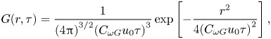 \begin{equation} G(r,\tau ) = \frac{1}{{{{(4{\rm \pi} )}^{3/2}}{{({C_{\omega G}}{u_0}\tau )}^{3}}}}\exp \left[ { - \frac{{{r^{2}}}}{{4{{({C_{\omega G}}{u_0}\tau )}^{2}}}}} \right] , \end{equation}
and its time integral is given by
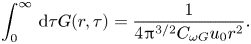 \begin{equation} \int_0^{\infty}\, {\mathrm{d}\tau } G(r,\tau ) = \frac{1}{{4{{\rm \pi} ^{3/2}}{C_{\omega G}}{u_0}{r^{2}}}} . \end{equation}
Gaussian functions similar to (4.24) were also used to study turbulent diffusion (Roberts Reference Roberts1961; Romanof Reference Romanof1989, Reference Romanof2006). As  $\tau$ increases, the peak value of
  $G(r,\tau )$ at
  $r=0$ decays and the width of the profile increases. Note that the width of the profile of
  $G(r,\tau )$ is proportional to
  $\tau$ and increases faster than
  $\tau ^{1/2}$ for an ordinary diffusion process. In fact, the temporal behaviour of
  $G(r,\tau )$ corresponds to a diffusion process with an effective diffusivity proportional to
  $u^{2}_{0}\tau$. Using (4.21) and (4.25), we can calculate the local eddy diffusivity
  ${\kappa _L}(=\kappa _{Lii}/3)$ as follows:
 \begin{align} {\kappa _L} &= \int\, {\mathrm{d}{\boldsymbol{r}}} {\kappa _{NL}}(r) = \int_0^{\infty}\, {\mathrm{d}r} 4{\rm \pi} {r^{2}}\frac{1}{{12{{\rm \pi} ^{3/2}}{C_{\omega G}}{u_0}{r^{2}}}}{Q_{ii}}({\boldsymbol{r}})\nonumber\\ &= \frac{{{u_0}}}{{3{{\rm \pi} ^{1/2}}{C_{\omega G}}}}\int_0^{\infty}\, {\mathrm{d}r} \frac{{{Q_{ii}}({\boldsymbol{r}})}}{{{Q_{ii}} ({\boldsymbol{0}})}} . \end{align}
The integral  $\int _0^{\infty }\, {\mathrm {d}r} {{{Q_{ii}}({\boldsymbol {r}})}}/{{{Q_{ii}}({\boldsymbol {0}})}}$ appearing on the right-hand side can be considered as an integral length scale
  $L$. Equation (4.26) shows that the local eddy diffusivity is proportional to the product of the turbulence intensity
  ${u_0}$ and integral length scale
  $L$; this relationship has often been discussed in turbulence modelling studies. This result indicates that the expression for
  $G(k,\tau )$, given by (4.23), is consistent with the conventional concept of the eddy diffusivity model.
For the velocity correlation  ${Q_{ii}}({\boldsymbol {r}})$, we assume the Kolmogorov spectrum in the inertial range following (2.17)–(2.19) for the TSDIA. The velocity correlation
  ${Q_{ii}}({\boldsymbol {r}})$ is given by
 \begin{gather} {Q_{ii}}({\boldsymbol{r}}) = \int\, {\mathrm{d}{\boldsymbol{k}}} {Q_{ii}}({\boldsymbol{k}})\exp (\mathrm{i}{\boldsymbol{k}} \boldsymbol{\cdot} {\boldsymbol{r}}) = \int_0^{\infty}\, {\mathrm{d}k} 2E(k)\frac{{\sin (kr)}}{{kr}} , \end{gather}
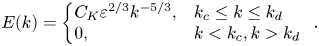 \begin{gather}E(k) = \left\{ \begin{array}{@{}ll} {{C_K}{\varepsilon ^{2/3}}{k^{ - 5/3}}}, & {{k_c} \le k \le {k_d}}\\ 0, & {k < {k_c},k > {k_d}} \end{array} \right. . \end{gather}
Here two cutoff wavenumbers are introduced,  ${k_c}\{ = {[{(3{C_K}/2)^{ - 1}}K{\varepsilon ^{ - 2/3}} + k_d^{ - 2/3}]^{ - 3/2}}\}$ in the energy-containing range and
  ${k_d}[ = {(3{C_K}/2)^{ - 3/4}}{\nu ^{ - 3/4}}{\varepsilon ^{1/4}}]$ in the dissipation range. The derivations of the two wavenumbers are presented in Appendix B. The profile of
  $E(k)$ with
  ${C_K} = 1.7$ is plotted as a red dotted line in figure 7(a). Finally, we obtain a model expression for
  ${\kappa _{NL}}(r,\tau )$ given by (4.20) with (4.24), (4.27) and (4.28).
Two model constants were used in the above model. Subsequently, the two sets of the constants listed in table 2 were considered. In model 1 a typical value of the Kolmogorov spectrum,  ${C_K} = 1.7$, is adopted. The value of
  ${C_{\omega G}} = 0.45$ was chosen such that the profile of
  ${\kappa _{NL}}(r,\tau )$ was close to the DNS value. The profiles of
  ${\kappa _{NL}}(r,\tau )$ are illustrated as red lines in figure 5. The profiles of model 1 show an overall agreement with the DNS values. This result indicates that the model expression for
  ${\kappa _{NL}}(r,\tau )$ derived above is reasonably accurate. The dependence of the model on
  $\tau$ is given by (4.24); it suggests a similarity law which makes the profile of
  ${\kappa _{NL}}(r,\tau )$ at a different time difference collapse to a single curve. The profile of
  ${r^{2}}{\kappa _{NL}}(r)$ is plotted as a red line in figure 4. This profile slightly underpredicted the DNS value in the entire region. By substituting (4.25) into (4.21), we obtain
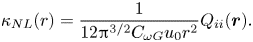 \begin{equation} {\kappa _{NL}}(r) = \frac{1}{{12{{\rm \pi} ^{3/2}}{C_{\omega G}}{u_0}{r^{2}}}}{Q_{ii}}({\boldsymbol{r}}) . \end{equation}
Therefore, the profile of  ${r^{2}}{\kappa _{NL}}(r)$ obtained using the model is proportional to
  ${Q_{ii}}({\boldsymbol {r}})$. Hence,
  ${r^{2}}{\kappa _{NL}}(r)$ for model 1 in figure 4 shows a small negative value at
  $r/L>2.6$, similar to the velocity correlation. Near
  $r=0$, the DNS value of
  ${r^{2}}{\kappa _{NL}}(r)$ is very small and is different from that of
  ${Q_{ii}}({\boldsymbol {r}})$. The small value of
  ${r^{2}}{\kappa _{NL}}(r)$ near
  $r=0$ is due to the viscous diffusion effect which was not incorporated into the present model (see Appendix C for details). We further evaluated the profile of
  ${\kappa _{NLyy}}(y - y')$ given by (4.22), which is visualised as a red line in figure 2. The profile for model 1 notably underpredicted the DNS value and it decreased more rapidly as
  $y - y'$ increased; the profile should be wider than that of model 1. Therefore, in model 1,
  ${\kappa _{NLyy}}(y - y')$ is too small, although
  ${\kappa _{NL}}(r,\tau )$ and
  ${r^{2}}{\kappa _{NL}}(r)$ agree with the DNS values.
Table 2. The values of model constants for the non-local eddy diffusivity  ${\kappa _{NL}}(r,\tau )$.

Let us next introduce model 2. In model 2 we changed the two model constants to improve the profile of  ${\kappa _{NLyy}}(y - y')$ within the framework of the proposed model expression. To obtain a wider profile, we decreased the cutoff wavenumber
  ${k_c}$ by choosing a smaller value of
  ${C_K} = 1.1$. The value of
  ${C_{\omega G}}$ was also modified, as shown in table 2. The profiles of
  ${r^{2}}{\kappa _{NL}}(r)$ and
  ${\kappa _{NL}}(r,\tau )$ for model 2 are plotted as blue dotted lines in figures 4 and 5, respectively. Although the profiles near
  $r = 0$ are less than the DNS values, the profiles at larger
  $r$ values were improved. The profile of
  ${r^{2}}{\kappa _{NL}}(r)$ for model 2 in figure 4 is better in the respect that it always shows a positive value like the DNS value, whereas that for model 1 shows a small negative value at
  $r/L>2.6$. Thus, in figure 2 the profile of
  ${\kappa _{NLyy}}(y - y')$ for model 2 agrees well with the DNS value. The scalar flux can then be expressed as
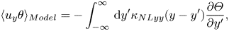 \begin{equation} {\langle {u_y}\theta \rangle _{Model}} ={-} \int_{ - \infty }^{\infty}\, {\mathrm{d} y'} {\kappa _{NLyy}}(y - y')\frac{{\partial \varTheta }}{{\partial y'}} , \end{equation}
where the profile of  ${\kappa _{NLyy}}(y - y')$ for model 2 was used. The profiles of
  ${\langle {u_y}\theta \rangle _{Model}}$ are depicted in figure 3 as green dotted lines. They also agreed well with the DNS values for all cases.
It is not clear why the profile of  ${\kappa _{NLyy}}(y - y')$ is better for model 2, although the overall profiles of
  ${r^{2}}{\kappa _{NL}}(r)$ and
  ${\kappa _{NL}}(r,\tau )$ are better for model 1. One reason can be the approximation given by (4.4). The deviatoric part of
  ${\kappa _{NLij}}({\boldsymbol {r}})$ in (4.3) may widen the profile, which should be examined in a future work. Another reason can be expressions of exponential form such as (2.16) and (4.15). Other functions may yield more successful descriptions of turbulent flows. Nevertheless, the present results clearly indicate the potential of the non-local eddy diffusivity model.
In this study we examined the DNS data of homogeneous isotropic turbulence, including the energy spectrum. An extension for inhomogeneous turbulence is an attractive future research program. However, Fourier transforms cannot always be applied to inhomogeneous turbulence with boundaries. The author recently proposed a formulation of the energy density in scale space instead of wavenumber space to examine inhomogeneous turbulence (Hamba Reference Hamba2022). It would be interesting to apply the formulation to the present analysis and modelling of the non-local eddy diffusivity for inhomogeneous turbulence. Another interesting study is the modelling of the non-local eddy viscosity for the Reynolds stress. Hamba (Reference Hamba2005) evaluated the non-local eddy viscosity using the DNS data of a turbulent channel flow, but its modelling has not been studied extensively. We expect that the present approach can also be applied to the non-local eddy viscosity.
5. Conclusions
A non-local expression for the turbulent scalar flux was investigated using the DNS data of homogeneous isotropic turbulence with an inhomogeneous mean scalar. In addition to the velocity field, the time evolution of scalar fluctuation was calculated for four cases with different mean scalar gradients. The profile of the non-local eddy diffusivity was obtained by evaluating Green's function for scalar fluctuation. It was verified that the non-local expression for the scalar flux agreed with the DNS value for all four cases. The local eddy diffusivity model overpredicted the DNS value because the scalar flux at a point is non-locally affected by the mean scalar gradient at remote points. The phenomenon of the counter-gradient diffusion, where the scalar flux and the mean scalar gradient have the same sign, also appeared because of the non-local effect.
The profile of the non-local eddy diffusivity was further analysed using the DNS data. In particular, profiles of the non-local eddy diffusivity at three time differences were obtained. It was shown that the spatial region where the mean scalar gradient non-locally affects the scalar flux widened as the time difference increased. A model expression for the non-local eddy diffusivity was proposed systematically in a manner customary in the statistical theory of turbulence. Following the DIA, we first assumed that the non-local eddy diffusivity was proportional to the two-point velocity correlation. Considering the DNS data of the velocity correlation and following the TSDIA, we further expressed the profiles of the energy spectrum and the time-dependent part. The profile of the non-local eddy diffusivity obtained from the model expression fairly agreed with the DNS value. Although the model expression underpredicted the one-dimensional non-local eddy diffusivity in the  $y$ direction, the profile was improved by adjusting the model constants such that the turbulence length scale could be longer. The results clearly indicate the potential of the non-local eddy diffusivity model. The analysis and modelling of the non-local eddy diffusivity provides insight into scalar transport in turbulence.
Funding
This work was supported by JSPS KAKENHI, grant number 20K04282.
Declaration of interests
The author reports no conflict of interest.
Appendix A. Transformation from three- to one-dimensional diffusivity
In § 2 we evaluated the one-dimensional profile of  ${\kappa _{NLij}}({r_y})$ as
 \begin{equation} {\kappa _{NLij}}({r_y}) = \langle {u_i}({\boldsymbol{x}},t){g_j}({\boldsymbol{x}},t;y')\rangle , \end{equation}
where
 \begin{equation} {g_i}({\boldsymbol{x}},t;y') = \int_{ - \infty }^{\infty}\, {\mathrm{d}\kern0.06em x'} \int_{ - \infty }^{\infty}\, {\mathrm{d}z'} \int_{ - \infty }^{t}\, {\mathrm{d}t'} {g_i}({\boldsymbol{x}},t;{\boldsymbol{x'}},t') . \end{equation}
Because the integrals with respect to  $x'$ and
  $z'$ are already included in (A2), a good statistical value of
  ${\kappa _{NLij}}({r_y})$ given by (A1) can be obtained by summing over a relatively small number of samples. We can also evaluate the three-dimensional profile of
  ${\kappa _{NLij}}({\boldsymbol {r}})$ as
 \begin{equation} {\kappa _{NLij}}({\boldsymbol{r}}) = \langle {u_i}({\boldsymbol{x}},t){g_j}({\boldsymbol{x}},t;{\boldsymbol{x'}}) \rangle, \end{equation}
where
 \begin{equation} {g_i}({\boldsymbol{x}},t;{\boldsymbol{x'}}) = \int_{ - \infty }^{t}\, {\mathrm{d}t'} {g_i}({\boldsymbol{x}},t;{\boldsymbol{x'}},t') . \end{equation}
Because the integrals with respect to  $x'$ and
  $z'$ are not included in (A4), it is necessary to sum over a large number of samples to obtain a good statistical value of
  ${\kappa _{NLij}}({\boldsymbol {r}})$ given by (A3).
In § 4, instead of evaluating  $\kappa _{NL}(r)(=\kappa _{NLii}({\boldsymbol r})/3)$ in (A3) directly, we first evaluated the one-dimensional profile of
  $\kappa _{NL}(r_{y})(={\kappa _{NLii}}(r_y)/3)$ in (A1) and transformed it into the three-dimensional profile of
  ${\kappa _{NL}}({r})$ as follows. Because
  ${\kappa _{NL}}(r)$ is a function of
  $r$ only, we can express
  ${\kappa _{NL}}({r_y})$ in terms of
  ${\kappa _{NL}}(r)$ as
 \begin{equation} {\kappa _{NL}}({r_y}) = \int_{ - \infty }^{\infty}\, {\mathrm{d}{r_x}} \int_{ - \infty }^{\infty}\, {\mathrm{d}{r_z}} {\kappa _{NL}}(r) = \int_{{r_y}}^{\infty}\, {\mathrm{d}r} 2{\rm \pi} r{\kappa _{NL}}(r) . \end{equation}
Conversely, by using (A5), we can express  ${\kappa _{NL}}(r)$ in terms of
  ${\kappa _{NL}}({r_y})$ as
 \begin{equation} {\kappa _{NL}}(r) ={-} \frac{1}{{2{\rm \pi} r}}{\left. {\frac{\partial }{{\partial {r_y}}}{\kappa _{NL}}({r_y})} \right|_{{r_y} = r}} . \end{equation}
Therefore, using the above relationship, we can evaluate  ${\kappa _{NL}}(r)$ from
  ${\kappa _{NL}}(r_{y})$ without summing over a large number of samples. Similarly, we can evaluate
  ${\kappa _{NL}}(r,\tau )$ from
  ${\kappa _{NL}}(r_{y},\tau )$ by using the relationship
 \begin{equation} {\kappa _{NL}}(r,\tau ) ={-} \frac{1}{{2{\rm \pi} r}}{\left. {\frac{\partial }{{\partial {r_y}}}{\kappa _{NL}}({r_y},\tau )} \right|_{{r_y} = r}} . \end{equation}
Appendix B. Energy spectrum in the inertial range
In the TSDIA described in § 2, the Kolmogorov spectrum was used for  $E(k)$ in the inertial range. In the energy-containing range,
  $E(k)$ should depart from the Kolmogorov spectrum and decrease to a smaller value as
  $k$ decreases. This behaviour of
  $E(k)$ was roughly approximated by the lower cutoff wavenumber
  ${k_c}$ in (2.17). The wavenumber
  ${k_c}$ was determined as follows. The integral of the energy spectrum should equal the turbulent kinetic energy as follows:
 \begin{equation} K = \int_0^{\infty}\, {\mathrm{d}k} E(k) = \int_{{k_c}}^{\infty}\, {\mathrm{d}k} {C_K}{\varepsilon ^{2/3}}{k^{ - 5/3}} = \frac{3}{2}{C_K}{\varepsilon ^{2/3}}k_c^{ - 2/3} . \end{equation}
This relationship yields the expression for  ${k_c}$ as
 \begin{equation} {k_c} = {\left( {\tfrac{3}{2}{C_K}} \right)^{3/2}}{K^{ - 3/2}}\varepsilon , \end{equation}
which was used in the TSDIA.
Strictly speaking, in the dissipation range,  $E(k)$ should also depart from the Kolmogorov spectrum and decrease exponentially as
  $k$ increases. In this study the profile of
  $E(k)$ is improved by considering not only the lower cutoff wavenumber
  ${k_c}$ in the energy-containing range, but also the higher cutoff wavenumber
  ${k_d}$ in the dissipation range. First, we considered the value of the dissipation rate which is given by the following integral:
 \begin{equation} \varepsilon = \int_0^{\infty}\, {\mathrm{d}k} 2\nu {k^{2}}E(k) \simeq \int_0^{{k_d}}\, {\mathrm{d}k} 2\nu {k^{2}}{C_K}{\varepsilon ^{2/3}}{k^{ - 5/3}} = \frac{3}{2}{C_K}\nu {\varepsilon ^{2/3}}k_d^{4/3} . \end{equation}
This relationship yields the expression for  ${k_d}$ as
 \begin{equation} {k_d} = {\left( {\tfrac{3}{2}{C_K}} \right)^{ - 3/4}}{\nu ^{ - 3/4}}{\varepsilon ^{1/4}} . \end{equation}
We then considered the value of the turbulent kinetic energy as
 \begin{equation} K = \int_0^{\infty}\, {\mathrm{d}k} E(k) = \int_{{k_c}}^{{k_d}}\, {\mathrm{d}k} {C_K}{\varepsilon ^{2/3}}{k^{ - 5/3}} = \frac{3}{2}{C_K}{\varepsilon ^{2/3}}(k_c^{ - 2/3} - k_d^{ - 2/3}) , \end{equation}
by adopting two cutoff wavenumbers. Thus,  ${k_c}$ can be determined by
 \begin{equation} {k_c} = {[ {{{( {\tfrac{3}{2}{C_K}} )}^{ - 1}}K{\varepsilon ^{ - 2/3}} + k_d^{ - 2/3}} ]^{{-}3/2}}. \end{equation}
This is slightly different from (B2) and involves the finite Reynolds number effect through  ${k_d}$. The two cutoff wavenumbers given by (B4) and (B6) were used in the energy spectrum in (4.28).
Appendix C. Green's function representing molecular diffusion
In figure 4 the profile of  ${r^{2}}{\kappa _{NL}}(r)$ at
  $r/L > 0.1$ was reproduced overall by the model expression, but the DNS value near
  $r = 0$ is small and clearly deviates from the model expression. This small DNS value can be understood by considering the viscous diffusion effect for a small time difference
  $\tau$ as follows. In § 4 we assumed that the profile of
  $G(k,\tau )$ is given by (4.23). This profile corresponds to a turbulent diffusion process with an effective diffusivity proportional to
  $u_0^{2}\tau$. Turbulent diffusion is caused by the convection term in the transport equation for
  ${g_i}({\boldsymbol {x}},t;{\boldsymbol {x'}},t')$ given by (2.7). For a small value of
  $\tau$, the effective diffusivity proportional to
  $u_0^{2}\tau$ becomes smaller than the molecular diffusivity
  $\kappa$. In such a case, the molecular diffusion term in (2.7) dominantly contributes to the time evolution of
  ${g_i}({\boldsymbol {x}},t;{\boldsymbol {x'}},t')$. Therefore, for a small value of
  $r[ < \kappa /({C_{\omega G}}{u_0})]$ corresponding to a small value of
  $\tau$, the profile of
  $G(k,\tau )$ should be expressed in the following form to represent the molecular diffusion
 \begin{equation} G(k,\tau ) = \frac{1}{{{{(2{\rm \pi} )}^{3}}}}\exp ( - \kappa {k^{2}}\tau ) , \end{equation}
instead of (4.23), which represents turbulent diffusion. In physical space, it is written as
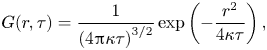 \begin{equation} G(r,\tau ) = \frac{1}{{{{(4{\rm \pi} \kappa \tau )}^{3/2}}}}\exp \left( { - \frac{{{r^{2}}}}{{4\kappa \tau }}} \right) , \end{equation}
and its time integral is given by
 \begin{equation} \int_0^{\infty}\, {\mathrm{d}\tau } G(r,\tau ) = \frac{1}{{4{\rm \pi} \kappa r}} . \end{equation}
Consequently, we have
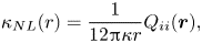 \begin{equation} {\kappa _{NL}}(r) = \frac{1}{{12{\rm \pi} \kappa r}}{Q_{ii}}({\boldsymbol{r}}) , \end{equation}
which differs from (4.29) by a factor of  $r$ and yields
  ${r^{2}}{\kappa _{NL}}(r) \propto r{Q_{ii}}({\boldsymbol {r}})$. Therefore, the profile of
  ${r^{2}}{\kappa _{NL}}(r)$ near
  $r = 0$ is not constant but is proportional to
  $r$, which is consistent with the profile plotted as a black line in figure 4.


 Open access