


1. Introduction
Flow around tandem cylinders has attracted considerable research interest both from an engineering point of view and among those who study the fundamentals of fluid mechanics. While there are now quite a number of investigations into this topic, its complex form of wake interference is still not fully understood. This is particularly true for the transition between tandem cylinder flow regimes, where the flow may be unstable and hysteretic (Carmo et al. Reference Carmo, Meneghini and Sherwin2010b).
Generally, there are three different regimes of tandem cylinder flow: overshoot, reattachment and co-shedding. These depend on the spacing between the cylinders and on the Reynolds number,  $Re = U_{0} D/ \nu$ (here, $U_{0}$ is the inflow velocity, $D$ is the cylinder diameter and $\nu$ is the kinematic viscosity of the fluid). When the cylinders are very close, the shear layers from the upstream cylinder envelop the downstream cylinder and roll up in the wake, so that vortex shedding occurs solely from the upstream cylinder. Increasing the spacing between the cylinders leads to reattachment of the upstream shear layers onto the downstream cylinder. Vortex shedding now occurs from the downstream cylinder. Reattachment may be alternating, quasi-steady/symmetrical or intermittent, from smaller to larger spacing (Zdravkovich Reference Zdravkovich1987). Further increase of the spacing will finally result in vortex shedding from both cylinders, so that there is a wake in the gap between them, i.e. co-shedding.
Due to Reynolds number dependency (Xu & Zhou Reference Xu and Zhou2004), it is challenging to give a consistent classification of tandem cylinder flow regimes based on the cylinder spacing alone. Still, the classification of Zdravkovich (Reference Zdravkovich1987) is commonly used: (a) overshoot/no reattachment  $1.0 \leq L/D \leq 1.2 -1.8$, (b) reattachment $1.2 -1.8 \leq L/D \leq 3.4 -3.8$ and (c) co-shedding $3.4-3.8 \leq L/D$. Here, $L/D$ is the centre-to-centre cylinder spacing, normally called the gap ratio, a term that will be used throughout the present paper from here on.
Reattachment may occur on the downstream or upstream side of the downstream cylinder. Based on this, Xu & Zhou (Reference Xu and Zhou2004) suggested that the reattachment regime should be subdivided (as well as extended with respect to the findings of Zdravkovich (Reference Zdravkovich1987)): in the range  $2 \leq L/D \leq 3$ there is a transition from overshoot to reattachment and in the range $3 \leq L/D \leq 5$ the flow transitions from reattachment to co-shedding.
The gap ratio at which co-shedding first occurs is traditionally called the critical spacing, or drag-inversion spacing. The latter term hails from the fact that, as long as there is shear layer reattachment, recirculation in the gap causes suction and results in a negative drag coefficient for the downstream cylinder. When co-shedding commences, the sign of the downstream cylinder drag coefficient is reversed, and becomes positive. Drag inversion typically occurs between  $L/D =$3.0 and 5.0 (Okajima Reference Okajima1979; Igarashi Reference Igarashi1981; Xu & Zhou Reference Xu and Zhou2004; Alam Reference Alam2014), depending on the Reynolds number, but also on factors such as free-stream turbulence (Ljungkrona, Norberg & Sunden Reference Ljungkrona, Norberg and Sunden1991) or inflow gust amplitude (Wang et al. Reference Wang, Zhou, Alam, Yang and Li2022), as well as the aspect ratio (Carmo, Meneghini & Sherwin Reference Carmo, Meneghini and Sherwin2010a). Higher ${{Re}}$ and increased non-uniformity of the inflow conditions favour transition at lower gap ratios. The effect of aspect ratio is related to the development of three-dimensionalities in the wake at moderate Reynolds numbers, which will be elaborated shortly. For further details regarding the co-shedding regime, the reader is referred to the reviews of Sumner (Reference Sumner2010) and Zhou & Alam (Reference Zhou and Alam2016).
Within the reattachment regime, there are recirculating vortices in the gap. For lower gap ratios, these tend to be symmetrical (Lin, Yang & Rockwell Reference Lin, Yang and Rockwell2002), but become alternating as the gap ratio increases (Carmo, Meneghini & Sherwin Reference Carmo, Meneghini and Sherwin2010b; Zhou et al. Reference Zhou, Alam, Cao, Liao and Li2019). Such vortices are often called quasi-stationary or quasi-steady in the literature, because their formation length is limited by the gap length, and thus they remain at essentially the same streamwise location. Herein, we call them ‘gap vortices’ or ‘recirculating vortices’ for simplicity. Igarashi (Reference Igarashi1981) discovered that close to the drag-inversion spacing, the gap vortices became unstable and shedding was detected intermittently (called regime D in that study). This is the beginning of a regime where the flow may switch intermittently between reattachment and co-shedding. The term ‘bi-stability’ was first used by Igarashi (Reference Igarashi1981) to describe this behaviour, and has been widely adopted since.
Bi-stability manifests as dual peaks in the velocity spectra. In the study of Igarashi (Reference Igarashi1981), for a given gap ratio, the peaks start out at similar frequencies, but move further apart as the Reynolds number increases. Based on the measured data, as well as flow visualisations, it was concluded that the flow exhibited two stable states (although it may perhaps be more accurate to call them conditionally stable), with one of them (reattachment) being ‘more stable than the other’. The number of occurrences of intermittent co-shedding and their duration increased with increasing Reynolds number and/or gap ratio.
Xu & Zhou (Reference Xu and Zhou2004) reported another type of bi-stable flow, namely a switch between stable overshoot and stable reattachment. For gap ratios 2.0, 2.5 and 3.0, this occurred within the Reynolds number ranges  ${{Re}} = 5 \times 10^{3} - 7 \times 10^{3}$, ${{Re}} = 4 \times 10^{3} - 7 \times 10^{3}$ and ${{Re}} = 3 \times 10^{3} - 6 \times 10^{3}$, respectively.
At first, the relationship between gap ratio, Reynolds number and tandem flow regimes received more interest than the three-dimensional characteristics of the flow field (Zdravkovich Reference Zdravkovich1972, Reference Zdravkovich1987; Lee & Basu Reference Lee and Basu1997; Xu & Zhou Reference Xu and Zhou2004; Zhou & Yiu Reference Zhou and Yiu2006; Alam et al. Reference Alam, Moriya, Takai and Sakamoto2003). This changed with three studies published nearly at the same time, independently of each other: Deng et al. (Reference Deng, Ren, Zou and Shao2006), Papaioannou et al. (Reference Papaioannou, Yue, Triantanfyllou and Karniadakis2006) and Carmo & Meneghini (Reference Carmo and Meneghini2006). Wake transition was the main interest of Deng et al. (Reference Deng, Ren, Zou and Shao2006) and Carmo & Meneghini (Reference Carmo and Meneghini2006), whereas Papaioannou et al. (Reference Papaioannou, Yue, Triantanfyllou and Karniadakis2006) also quantified three-dimensional effects and spanwise variations. A common conclusion of all three investigations was that two-dimensional numerical simulations fail to predict the correct drag-inversion spacing for a three-dimensional wake. Moreover, both Deng et al. (Reference Deng, Ren, Zou and Shao2006) and Papaioannou et al. (Reference Papaioannou, Yue, Triantanfyllou and Karniadakis2006) note that the downstream cylinder may partially or completely suppress three-dimensionality when placed within the drag-inversion spacing. This corresponds well to previous observations that transition to turbulence in the wake occurred later, in terms of Reynolds number, for tandem cylinders within the reattachment regime, than for a single cylinder (Zdravkovich Reference Zdravkovich1972).
The work of Carmo & Meneghini (Reference Carmo and Meneghini2006) was later expanded to include a classification of secondary instabilities in tandem cylinder wakes (Carmo et al. Reference Carmo, Meneghini and Sherwin2010b) and the relation between the onset of these instabilities and transition between tandem cylinder flow regimes (Carmo et al. Reference Carmo, Meneghini and Sherwin2010a). Three different secondary instability mechanisms for tandem cylinders were identified, T1–T3. The third type is most pertinent to the present study, as we shall soon see, because, among the different three-dimensional instabilities, only T3 originates in the gap. Carmo et al. (Reference Carmo, Meneghini and Sherwin2010b) argue that this mode is kindred to the mode A (Williamson Reference Williamson1996) of single cylinders (albeit with oppositely signed streamwise vorticity). Their reasoning is that the underlying physical mechanism, namely a cooperative elliptical instability, is the same. The cooperative nature of the instability, meaning that it depends on interaction between the shear layers, was verified by placing a splitter plate in the far end of the gap. This was seen to obliterate three-dimensionality altogether for  $L/D = 2.3$, $Re = 300$.
Regarding drag inversion and wake transition predictions, it is the characteristic perturbation wavelength of the three-dimensional instabilities that causes the discrepancy between two-dimensional and three-dimensional simulations, as well as between studies with low and high aspect ratios. For instance, Carmo et al. (Reference Carmo, Meneghini and Sherwin2010a) report that, for  $L/D = 3.5$, the onset of T3 occurs at ${{Re}} = 217$, with a wavelength of $9.97 D$. In comparison, Deng et al. (Reference Deng, Ren, Zou and Shao2006) report onset of three-dimensionality at ${{Re}} = 250$, with a mode A structure. Carmo et al. (Reference Carmo, Meneghini and Sherwin2010a) argue that Deng et al. (Reference Deng, Ren, Zou and Shao2006) could not capture mode T3 because of insufficient spanwise domain length.
The three-dimensional wake instability causes waviness of the spanwise vortex cores, and this waviness gives rise to phase differences in the flow field, as observed by Papaioannou et al. (Reference Papaioannou, Yue, Triantanfyllou and Karniadakis2006). In their case with  $L/D = 2$ and $Re = 500$, both gap and wake show clear evidence of periodic spanwise structures. A similar result was recently reported by Wang et al. (Reference Wang, Liu, Li and Xu2021) for channel-confined tandem cylinders.
The existence of spanwise phase differences implies the possibility of variation between different tandem flow regimes along the cylinder span, near the drag-inversion spacing. This idea was put forth by Aasland et al. (Reference Aasland, Pettersen, Andersson and Jiang2022), who suggested that bi-stability may occur in spanwise cells, based on the observation of spanwise inhomogeneity at  $L/D = 3$ and $Re = 10\,000$. In the present study, we have investigated this hypothesis. A Reynolds number of 500 was chosen, in order to ascertain that the flow regime was far away from transition between different three-dimensional instabilities. The gap ratio was kept at $L/D = 3$. According to Carmo et al. (Reference Carmo, Meneghini and Sherwin2010a), the present study should be well within the region of T3. Moreover, using a lower Reynolds number allowed for a long spanwise length while keeping the computational cost manageable. Tandem cylinders near the drag-inversion spacing bring together several fundamental phenomena of bluff-body fluid mechanics, and the outcome of the computation will enable an in-depth exploration of the surprisingly complex vortex dynamics in this particular flow regime.
2. Problem formulation and computational approach
2.1. Governing equations and numerical method
In the present study, the incompressible continuity and Navier–Stokes equations are solved by means of direct numerical simulations (DNS). The governing equations are
 \begin{gather} \frac{\partial u_{i}}{\partial x_{i}} = 0, \end{gather}
 \begin{gather} \frac{\partial u_{i}}{\partial t} + u_{j} \frac{\partial u_{i}}{\partial x_{j}} =-\frac{1}{\rho} \frac{\partial P}{\partial x_{i}} + \frac{\partial}{\partial x_{j}} \left( \nu \left[ \frac{\partial u_{i}}{\partial x_{j}} + \frac{\partial u_{j}}{\partial x_{i}} \right] \right),\quad i,j = 1,2,3, \end{gather}
where  $u$ is velocity, $P$ is pressure and $\rho$ is fluid density. The simulation was carried out using the MGLET (Multi Grid Large Eddy Turbulence) flow solver. MGLET is based on a finite volume formulation of the incompressible Navier–Stokes equations, and uses a staggered Cartesian grid (Manhart Reference Manhart2004). Solid bodies are introduced through an immersed boundary method (Peller et al. Reference Peller, Le Duc, Tremblay and Manhart2006), where the boundary is discretised using a cut-cell approach. A third-order low-storage explicit Runge–Kutta time integration scheme is used for time stepping, and the Poisson equation is solved using an iterative, strongly implicit procedure.
Periodic boundary conditions were used in the spanwise direction, and a free-slip condition was used on the top and bottom boundaries ( $y$-direction, see figure 1a). Uniform inflow was imposed at the inlet, and a Neumann condition was imposed on the velocity components at the outlet.

Figure 1. Computational domain and (b) grid schematic.
In order to accelerate the development of the flow field, a turbulence intensity of 0.2 % was imposed in the domain for a short time, at the very beginning of the simulation. Sampling of statistics started after 100 convective time units ( $U_{0}/D$). Before sampling commenced, the time step was gradually adjusted to obtain a target Courant number of 0.5. The final non-dimensional time step was ${\rm d}t = 2.0562 \times 10^{-3}$. Statistics were sampled for 800 time units, which amounts to around 114 vortex shedding cycles.
2.2. Computational domain and grid
The computational domain and a schematic view of the grid are displayed in figure 1. The inflow boundary is located at  $x/D = -15$. The grid is refined in nested boxes, as shown in figure 1(b), where each child box has half the cell size of its parent. The nested grid structure is the reason for the seemingly arbitrary domain size, since each dimension must be an integer multiple of the largest grid cell size. There were six grid levels in total, and the smallest grid cell size was ${{\rm d}\kern0.7pt x} = {{\rm d} y} = {\rm d}z = 0.0075D$. This gives a total number of grid cells of nearly $1.4 \times 10^{9}$. The innermost grid refinement box is $2.5D$ long in the $y$-direction (symmetrical about $y/D = 0$), and stretches from $x/D = -0.63$ to $x/D = 7.0$. The finest grid spans the entire domain i $z$-direction.
A grid convergence study has not been carried out specifically for the purpose of this investigation. However, in our previous study with a Reynolds number of 10 000, a grid cell size of  $0.005D$ gave good results (Aasland et al. Reference Aasland, Pettersen, Andersson and Jiang2022). Therefore, we are confident that a similar cell size will be sufficient also at the present Reynolds number, which is nearly two orders of magnitude lower.
The effect of spanwise length and spanwise boundary conditions on the flow field was assessed, without any change of the grid cell size and distribution. A pair of simulations were carried out initially, using a spanwise domain size of  $L_{z} = 7.68D$. One case used periodic spanwise boundary conditions, and the other used free-slip spanwise boundary conditions. Statistical sampling time was 700 and 600 time units, respectively. The results are listed in table 1, and it is clear that the main statistical quantities are quite robust, with differences of the order of 1 % or 2 %. The use of free-slip walls more than doubles the value of the spanwise force fluctuations, however. For the periodic $L_{z} = 7.68D$ case, the values are $C_{zrms} = 3.1 \times 10^{-4}$ and $6.7 \times 10^{-4}$, for the upstream and downstream cylinders, respectively, whereas for the free-slip case, the corresponding values are $C_{zrms} = 7.9 \times 10^{-4}$ and $17.2 \times 10^{-4}$. This increase of spanwise force fluctuations is reflected in the spanwise velocity fluctuations, and gives rise to more frequent occurrences of the second gap vortex mode described in § 3.2.
Table 1. Main statistics compared with results in the literature. Here,  $\theta _{r}$ denotes the reattachment angle (see figure 2).

In the case of periodic spanwise boundary conditions, there is virtually no difference in the main statistics between  $L_{z} = 7.68D$ and $15.36 D$. Thus, $L_{z} = 7.68D$ is possibly sufficient in order to capture the physics of the present case. It was the wholly unexpected observation of the long-term gap asymmetry, detailed in § 3.2, that precipitated the doubling of the spanwise domain size. The asymmetry was initially believed to be an effect of numerical perturbations related to the spanwise length, but was found to be a real physical phenomenon. Despite the increased computational cost, we decided to continue with $L_{z} = 15.36D$ in order to get a better overview of the complex spanwise variations of the flow field.
Finally, the spanwise coherence described in § 3.3 occurred once during the  $L_{z} = 7.68D$ periodic simulation, but not for the free-slip simulation. This may be due to the duration of the simulation, and we cannot conclude on whether it is an effect of the boundary conditions.
2.3. Definitions
The time-averaged base pressure coefficient is given as  $\bar {C}_{pb} = ( \bar {P} - \bar {P}_{0} ) / (\bar {P}_{s} - \bar {P}_{0})$. Here, $\bar {P}_{0}$ is the pressure at the inlet and $\bar {P}_{s}$ is the stagnation pressure. Force coefficients are defined as $C_{F} = 2F/\rho U_{0}^{2} A$, where $F$ is the force component in question, $\rho$ is the fluid density and $A$ is the projected frontal area. The lift coefficient is given by its root mean square (r.m.s.) value. Subscripts $D$ and $L$ denote drag and lift, respectively. To separate the upstream and downstream cylinder coefficients, lower case $u$ and $d$ subscripts are used. The Strouhal number is defined as $St = f_{v}U_{0}/D$, where $f_{v}$ is the von Kármán vortex shedding frequency.
Herein, spectral analysis has been carried out by means of fast Fourier transform (FFT) of velocity time traces from a set of probes in the wake and gap. These probes have an internal spacing of  $0.03D$, which corresponds to the grid resolution on the third finest grid level. The frequency resolution was approximately $0.0012U_{0}/D$.
3. Results
3.1. Overview of the flow topology
In the present study, with  $L/D = 3.0$ and
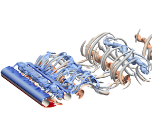
  ${{Re}} = 500$, the basic tandem cylinder flow regime is alternating overshoot/reattachment, where the reattachment points are located on the upstream side of the downstream cylinder, as illustrated in figure 2. Recirculating vortices form alternatingly in the gap. The gap shear layer which is not undergoing roll-up overshoots the downstream cylinder and merges with its shear layer in the near wake. The shear layers are laminar and transition to turbulence occurs in the wake. Figure 3 gives an instantaneous view of the flow topology. In both the gap and wake, the flow exhibits strong three-dimensional features. Streamwise vortical structures bridge the von Kármán vortices, forming loops: this is the three-dimensional instability T3, as described by Carmo et al. (Reference Carmo, Meneghini and Sherwin2010b) (see figure 3, inset B).

Figure 2. Basic flow regime, i.e. alternating reattachment/overshoot, illustrated by a snapshot at  $tU_{0}/D = 126.23$, $z/D = 1$. Recirculating vortices alternate in the gap. The gap shear layer which is not rolling up overshoots the downstream cylinder, merging with its shear layer. The instantaneous location of shear layer reattachment is marked in the figure. The time-averaged position of this point is denoted $\theta _{r}$. The small circles mark probe lines used for sampling velocity data for spectral analysis; P1 and P2 are located at $(x/D, y/D) = (1.98, 0.60)$ and $(x/D, y/D) = (2.49, 0.60)$, respectively, P3 is located at $(x/D, y/D) = (4.50, 0.65)$ and P4 at $(x/D, y/D) = (2.49, -0.60)$.

Figure 3. Instantaneous view of the lower shear layer at  $tU_{0}/D = 800.77$. The flow field is visualised by isosurfaces of $Q(D/U_{0})^{2} = 0.05$, coloured by the spanwise vorticity. Inset A shows an unstable vortex cell coloured by the streamwise vorticity. Here, $Q(D/U_{0})^{2} = 1$ is used. Mode T3 type vortical structures are shown in inset B. Inset C shows secondary vortices in the near wake. The formation process of such vortices is illustrated in figure 7.
The main statistics are listed in table 1, and there is good agreement between the present study and results from the literature.
The flow is clearly bi-stable, with two modes that have distinct Strouhal numbers. This is seen from the velocity spectra in the gap and wake, shown in figure 4. The Strouhal number is  $St \approx 0.14$ ( $0.140$ from probe lines P1 and P2 in the gap and $0.143$ from probe line P3 in the wake), whereas the secondary mode has a slightly higher frequency, with a peak near $0.155$. The existence of a second mode has been verified by spectral analysis of the forces, although these plots are not shown herein. The second mode is associated with a stronger dynamics in the gap and intermittent shedding of gap vortices, as well as overshoot of the gap shear layers further into the near wake, and wider gap and wake widths. This is shown in the supplementary movie 1 available at https://doi.org/10.1017/jfm.2023.468 (the second mode starts around $tU_{0}/D = 379$). This flow regime is very similar to observations of Igarashi (Reference Igarashi1981) and Kitagawa & Ohta (Reference Kitagawa and Ohta2008) for $L/D \approx 3.0$, although these have significantly higher Reynolds numbers.

Figure 4. Spanwise-averaged cross-flow velocity spectra in the gap at (a) P1 and (b) P2, and in the wake at (c) P3 (see figure 2 for exact probe locations). The insets show a close up of the main peak, so that the secondary peaks can be distinguished. Flow bi-stability manifests as a secondary spectral peak at approximately  $fD/U_{0} = 0.155$.
Similar to the findings of Papaioannou et al. (Reference Papaioannou, Yue, Triantanfyllou and Karniadakis2006) and Wang et al. (Reference Wang, Liu, Li and Xu2021), the gap is organised into spanwise cells with a length of approximately  $2.5D$ to $3.8D$. This is clearly seen in the time-averaged streamwise and spanwise velocity fields, shown in figures 5(a) and 5(b), respectively. The largest observed cell length is comparable to that of the previous studies, which is approximately $4D$ for Reynolds numbers 500 and 400 (Papaioannou et al. Reference Papaioannou, Yue, Triantanfyllou and Karniadakis2006; Wang et al. Reference Wang, Liu, Li and Xu2021). Note that the cell length value was gleaned from instantaneous plots in those studies, and we do not possess information regarding variation or time-averaged values. The spanwise cells of the present study and their locations are quite persistent in time in both gap and near wake, as shown in figure 6. The horizontal stripes of similar magnitude $C_{pb}$ show the cells, their centres being the regions of lowest magnitude. The time-averaged cell boundaries are marked by dashed lines. We see that there is some meandering and merging of the instantaneous cells, perceived as ‘dislocations’ or blurred areas. Some of these are highlighted by dashed ovals in figure 6(a).

Figure 5. Time-averaged velocity field in the gap and near wake, in the plane  $y/D = 0$. Panels (a–c) are averaged over the entire duration of the simulation, whereas (d–f) are averaged over $378 \leq tU_{0}/D \leq 493$, which corresponds to approximately 16.4 vortex shedding cycles. The spanwise cell structure is marked by dashed lines. The cell boundaries are defined by sign switch of $W/U_{0}$ in the gap. The averaged cross-flow velocity is non-zero in the gap, due to persistent asymmetry of the gap vortices, as described in § 3.2. In (e), this asymmetry is coherent along the span, which is connected with increased drag amplitude, as shown in figure 10(b).

Figure 6. Instantaneous base pressure coefficient of the (a) upstream and (b) downstream cylinders, calculated from probe data along the line  $(x/D,y/D) = (0.51,0)$. The spanwise distribution clearly shows cells that are persistent in time, and remain in nearly the same spanwise location for long periods. The dashed lines mark the boundaries of the time-averaged cell structure, given in figure 5(a). The dashed ovals mark intervals of cell ‘dislocations’. Note that (a,b) use different scales, in order to enhance the cell structures. (Due to an output writing error, data are missing in the time interval $611 \leq tU_{0}/D \leq 625$.)
The differences in phase and structure caused by the basic spanwise organisation are significant. Figure 7 shows a series of flow snapshots taken over one vortex shedding period, in the planes  $z/D = 0$ and $z/D = 1$. Considering that these spanwise locations are separated only by one diameter, the variation is striking. Most obvious to the eye, is that at $z/D = 0$ (left-hand panels of figure 7) there is a strong roll-up of the upper shear layer during this interval, while at $z/D = 1$ (right-hand panels of figure 7) the same occurs, but in the opposite (lower) shear layer. There are also differences in phase and strength of the wake vortex shedding, but these are less profound than those of the gap. In the inset of figure 7, the spanwise velocity has been averaged over $351.54 \leq tU_{0}/D \leq 358.51$. The plot indicates that $z/D = 0$ and $z/D = 1$ are located in different spanwise cells during this interval, with $z/D = 1$ being very close to the boundary of its cell. This is one of the main reasons for the observed differences. Another important factor is the existence of unstable gap shedding cells, which will be elaborated in § 3.2.

Figure 7. Instantaneous flow during one vortex shedding period, represented by  $\omega _{z} D/ U_{0}$, in the planes $z/D = 0$ and $z/D = 1$. A secondary vortex is marked by the dashed oval, and interaction between secondary vortices is shown in (h i), marked with a dashed rectangle. There are significant differences in the vortical structures of the two planes, even if they are a mere diameter apart. This is likely because the planes are located in different spanwise mother cells, as indicated in the inset, which shows the time-averaged spanwise velocity during this vortex shedding period.
Inset C in figure 3 shows the existence of secondary gap vortices, which are created through interaction between the overshooting gap shear layer and near wake. The formation process is highlighted in figure 7(a ii–h ii). A video of this time interval is available in supplementary movie 2. In the first snapshot, figure 7(a ii), the lower gap shear layer has begun to roll up after previously overshooting into the near wake. The roll-up starts with a concentration of vorticity forming well upstream of the downstream cylinder. This causes the downstream part of the gap shear layer (marked by a dashed oval), which extends beyond the gap, to be pinched off. The process is amplified, in this case, by a remnant of the previous gap vortex, marked by a black arrow. In figure 7(c ii), the pinched-off gap shear layer has been completely cut loose, and continues to roll up into a secondary vortex as it is convected downstream. This makes it appear as though the period of the von Kármán vortex street is doubled on just one side of the wake, as seen in figure 7(g ii,h ii). In inset C of figure 3, however, we see that this type of vortex has a very short spanwise length (the spacing between the legs of these horseshoe vortices is around  $1D$), and their primary effect is to increase the overall three-dimensionality in the wake. To our knowledge, this is the first time such vortices are described in the literature.
3.2. Unstable children: shedding in short spanwise cells
We have discovered that bi-stability may indeed be cellular, as suggested by Aasland et al. (Reference Aasland, Pettersen, Andersson and Jiang2022). Local manifestations of the mode switch emerge clearly from the velocity time traces in figure 8. It is evident that the second mode does not as a rule occur simultaneously at different spanwise locations. Moreover, the mode appears to be asymmetric with respect to the midplane  $y/D = 0$, which is seen when comparing the time traces from two probes on opposite sides of the gap, shown in figure 8(a iii,b). It must be mentioned that occurrences of the second mode can be quite brief, typically one or two periods, but occur often during a given time interval. In figure 8, the vertical dashed lines mark the boundaries between time intervals where the time traces predominantly display the first or second mode.

Figure 8. Velocity time history at the end of the gap, at (a) P2 and (b) P4 for  $z/D = 0$, and (c) P2 for $z/D = -6$. For brevity, only $w/U_{0}$ is shown in (b,c). The mode switch manifests asymmetrically and locally, so that different spanwise locations do not always exhibit the same mode. Even at a given spanwise location there can be large differences between the upper and lower gap shear layers, as seen when comparing (a iii,b).
In the gap, vortex shedding occurs in relatively short spanwise cells. Such a cell is shown in inset A of figure 3. This particular cell consists of three small horseshoe vortices, and has a spanwise length of approximately  $0.75D$. Our observations indicate that the unstable cells appear within the boundaries of the basic spanwise cell structure, and their length does not exceed the basic cell length. For this reason the basic cells and the unstable cells can be considered as ‘mother’ and ‘child’ structures, respectively.
A simplified method was used for estimating the length of unstable children, taking velocity data from probe line P2 (see figure 2). For each time a gap vortex formed on this side of the gap, the point of minimum cross-flow velocity ( $v_{min}$) was found. If $v_{min}$ was less than $-$0.5, this was assumed to be an unstable child. The cell length was then taken to be the spanwise extent around the location of $v_{min}$ where the condition $v/U_{0} \leq 0.9v_{min}$ was satisfied. Both the location of the probe line and the velocity constraint were chosen empirically. This method has some obvious drawbacks, one of them being that only one cell is estimated during each period, although cells may appear at several spanwise locations. With the long sampling time, however, there were still ample events on which to base an estimate. The cell length varies considerably, going from $0.3D$ to $2.7D$. However, an overall average of $0.78D$ implies that most cells are quite short.
Intriguingly, unstable children may manifest themselves in the same location, with reasonably similar cell length for several consecutive periods. An example of this is shown in figure 9, where the cells are visualised by means of the cross-flow velocity. Here, an unstable child appears in the same spanwise location for five successive periods. The child maintains approximately the same cell length throughout, except at  $tU_{0}/D = 229.48$, where it has grown somewhat. This cell is centred around $z/D = 6$, whereas another significantly smaller and weaker structure is centred near $z/D = 3$.

Figure 9. Cross-flow velocity in a plane in the gap, at  $y/D = 0.6$. During the time interval shown, vortex cells of similar cell length recur at the same spanwise location over five vortex shedding periods. These events are marked by a big dashed rectangle. A smaller rectangle marks a weaker recurring structure. Gap shedding occurs within the boundaries of the mother cell, which is likely the reason for the consistent location. When roll-up occurs in the gap, high-momentum fluid is pulled into the recirculation region and this contributes to maintaining the gap shedding mode over several periods.
The recurrence of unstable children leads to asymmetry with respect to the  $y$ axis in the gap, as shown in the time traces in figure 8, so that strong vortices are formed repeatedly on one side of the gap for long intervals. This inevitably skews the velocity field, and has the practical consequence that the time-averaged cross-flow in the gap centreplane takes a long time to reach zero, as one would expect from experience with single cylinder vortex shedding. In fact, it may theoretically never do so, seeing as the asymmetry manifests randomly. This is illustrated in figure 5(b), where the cross-flow velocity in the gap is seen to have a cellular structure which is different from the mother cells.
Given that the switch between reattachment and shedding is assumed to be a random process, it is indeed curious, and seemingly a paradox, that an unstable child should reappear in the manner that we have observed. However, we believe the explanation is a simple one: the first occurrence in a series of gap vortex shedding events is truly random, the result of triggering the instability in the gap. Meanwhile, when the gap vortex rolls up early, i.e. away from the surface of the downstream cylinder, this opens the gap recirculation region so that high-momentum fluid from the outside can first be entrained and subsequently recirculated. In turn, this fluid amplifies the instability and triggers repeated shedding events, until equilibrium is reached once more. From the visualisations (see movie 3,  $tU_{0}/D \approx 670$), we see that recirculating fluid entrained by strong gap vortices will sometimes impinge on the shear layer on the same side of the gap at which it was entrained. This way, it enhances the roll-up process. Lower-momentum entrained fluid is mostly swallowed by the gap vortex forming on the opposite side.
It must be emphasised here that the gap shedding is different from the regular vortex shedding process (as detailed by Gerrard Reference Gerrard1966), because the downstream cylinder impedes communication between the shear layers. The growing gap vortex is not able to draw the opposite shear layer fully across the gap, although fluid of oppositely signed vorticity does cross the centreline. As a result, the vortex is not cut off by the opposing vortex; rather it is convected downstream by the high-momentum fluid outside the gap. This is what allows the feedback mechanism which causes unstable child recurrence; that not all the recirculating fluid is entrained and shed during a single period. The formation length, in the instantaneous sense, of the shed vortices is not very different from the recirculating gap vortices, and that causes their primary frequencies to be quite close to one another.
3.3. Spanwise mode coherence
In figure 10(a,b), the time traces of the drag coefficients (in particular the downstream coefficient  $C_{Dd}$) have intervals of strong oscillations, their duration ranging from a couple of vortex shedding periods up to 16–20 periods. These intervals are associated with overall increased velocity fluctuations. We have compared the spanwise-averaged r.m.s. of the velocity fluctuations in the time interval $378 \leq tU_{0}/D \leq 493$ with those of $100 \leq tU_{0}/D \leq 215$, during which $C_{Dd}$ has relatively low-amplitude fluctuations. In the gap, at P2 the increase of spanwise-averaged $u_{rms}$, $v_{rms}$ and $w_{rms}$ is 4.69, 34.82 and 26.31 %, respectively. In the wake, at P3, the corresponding changes are $-1.11$, 1.87 and 17.31 %.

Figure 10. Time histories of (a) upstream and (b) downstream drag coefficients, and (c) wavelet map of  $C_{Dd}$. The shaded region of the wavelet map marks the cone of influence. The flow is bi-stable throughout the time series, but intervals of strong $C_{Dd}$ oscillations are associated with increased spanwise coherence of the second mode. A snapshot of the flow near $tU_{0}/D = 385$ in figure 11 illustrates this mechanism. Periods of strong fluctuations are accompanied by an increase of spectral energy in the low-frequency components, which are related to variation of the reattachment and separation points on the downstream cylinder, as indicated in figure 13. (Aberrations due to the output writing error have been masked in the wavelet map.)
The value of  $C_{Dd}$ remains negative throughout the entire simulation, although it nearly reaches zero on two occasions (marked in figure 10b). This implies that the flow remains within the reattachment regime, although vortex shedding occurs locally along the span. Near-zero values of $C_{Dd}$ are accompanied by peaks in $C_{Du}$ (figure 10a). The strong oscillations occur primarily in the drag force, and there is no indication of a corresponding amplitude increase in the lift time traces, shown in figure 12(a,b).
During the intervals of strong oscillations, there is increased spanwise coherence of the asymmetry in the gap, which is of great interest. An example is shown in figure 5(e), where the cross-flow velocity field has been averaged over approximately 16.5 vortex shedding cycles. In this plot, as opposed to the all-time average in figure 5(b), the mother cells emerge quite clearly and the asymmetry has the same sign along the entire span. Positive velocity in the centreplane towards the end of the gap implies that the vortex in the upper shear layer is stronger than its opposite, and thus has a more concentrated core. The opposite weaker vortex has a larger diameter, and thus expands above the centreplane. It must be noted that not all intervals are as strongly coherent as this one, but the tendency is clear.
Figure 11 gives an instantaneous view of the flow at a time when  $C_{Dd}$ is close to a local maximum ( $tU_{0}/D \approx 385$, marked in figure 10b). We see that there is a large number of unstable children in the upper shear layer, spread along the entire cylinder span. The streamwise and cross-flow velocity components are largely coherent along the span, except near $z/D = -3$. Here, the cross-flow and spanwise velocities indicate the presence of a comparably strong vortex loop in the near wake, which influences the gap region and disrupts the coherence, likely through secondary structures.
These results indicate that the intervals of strong oscillations of  $C_{Dd}$ are not a mode change per se, but arise when spanwise localised occurrences of the second mode are somehow coordinated, so that the spanwise coherence increases. Vortex roll-up in the gap at several spanwise locations necessarily leads to an increase of the (negative) drag. Conversely, spanwise coherent reattachment causes local drag minima.

Figure 11. Snapshot of the flow at  $tU_{0}/D = 385.75$. This time instant corresponds to a peak in $C_{Dd}$, which is likely due to spanwise coherence of the second mode. (a) Shows that the streamwise and cross-flow velocities are largely coherent in the gap. Unstable children in the top gap shear layer are marked by dashed rectangles in (b). Panel (c) illustrates strong roll-up in the gap at this time instant. When the gap shear layers detach from the downstream cylinder, this increases $C_{Dd}$, as observed in figure 10(b). A strong vortex loop disrupts the spanwise coherence near $z/D = -3.0$, as shown in (a). The velocity scale is exaggerated to make the spanwise structures clear; (a) $y/D = 0$, (b) $y/D = 0.6$, (c) $z/D = 0$.
The significant increase of spanwise velocity fluctuations in both gap and wake is attributed to the three-dimensional instability T3, which is given more space to develop during the second mode.
Comparing the  $C_{Dd}$ and velocity time histories in figures 10(b) and 8, it is obvious that there is not always a correspondence between the increased force oscillations and velocity fluctuations at a given point. This is due to the cellular manifestation of the gap shedding. Plainly put, low fluctuations at the point probe combined with high fluctuations of the total drag force simply means that the mode switch occurs elsewhere along the span.
Although there is no appreciable impact of the second mode coherence on the downstream cylinder lift, the gap asymmetry influences the lift coefficient of the upstream cylinder, giving it a meandering, non-zero mean. This is clearly shown in figure 12. For example, during the time interval  $373 \leq tU_{0}/D \leq 493$, the mean lift in the upstream cylinder is negative, with a value of $\bar {C}_{Lu} = -0.013$. A positive mean value is observed during $720 \leq tU_{0}/D \leq 890$, which is another time interval of significant spanwise coherence of the second mode, with $\bar {C}_{Lu} = 0.012$.

Figure 12. Time history of (a) upstream and (b) downstream cylinder lift coefficients. The second mode coherence has no obvious influence on  $C_{Ld}$, but $C_{Lu}$ is influenced by long-term asymmetry in the gap, so that the mean value is non-zero. Panels (c,d) show time traces in the $C_{D}-C_{L}$ plane for the upstream and downstream cylinders, respectively.
Phase diagrams of drag and lift are given in figure 12(c,d), for the upstream and downstream cylinders, respectively. The drag time histories of both cylinders contain multiple periods, and the quasi-periodicity of the upstream cylinder lift results in an irregular path in the  $C_{D} - C_{L}$ plane, as shown in figure 12(c); $C_{Ld}$ is considerably less irregular than $C_{Lu}$, and its increased periodicity is evident in figure 12(d).
3.4. Low-frequency variations
When the first part of the simulation,  $100 \leq tU_{0}/D \leq 800$, was evaluated, it was discovered that there are low-frequency peaks in the velocity spectra. Therefore, the simulation was run for 100 additional time units while an in situ FFT was carried out. A spectral map of selected frequencies are shown in figure 13.

Figure 13. Spectral maps in the planes  $y/D = 0$ and $z/D = 6$, analysed over the time interval $800 \leq tU_{0}/D \leq 900$. Panels (a,b) show that there is low-frequency modulation of the reattachment and separation points on the downstream cylinder, which leads to slow variation of the vortex formation length. During this time interval, which covers approximately 14 von Kármán cycles, the gap vortex formation at $z/D = 6$ is clearly asymmetric, favouring the lower vortex. The approximate boundaries of the mother cells are marked by dashed lines. Note that due to strong variation in spectral energy, the scales are not the same for all plots; (a) $fU_0/D=0.02$, (b) $fU_0/D=0.04$, (c) $fU_0/D=0.12$, (d) $fU_0/D=0.14$.
Figure 13(a,b) display spectral maps of the lowest analysed frequencies,  $fD/U_{0} = 0.02$ and $0.04$, respectively. The plots in the plane $z/D = 6$ show that the gap vortex in the lower shear layer was stronger during the time interval analysed. In figure 13(a), the spectral density is concentrated mostly around this gap vortex and the reattachment point on the same side. There are density concentrations in the corresponding points on the opposite side, but these are weak in comparison.
Meanwhile, figure 13(b) displays density concentrations around the downstream cylinder separation points, as well as around the reattachment point and the lower gap vortex. For the separation points, the highest spectral density is found on the opposite side of the strong gap vortex, and this indicates a relation with the gap shear layer overshoot mechanism.
Both  $fD/U_{0} = 0.02$ and $0.04$ have energy content in the near wake, but the distributions are different. In figure 13(a), we see that, in the near wake, the spectral energy is skewed towards the opposite side of the strong gap vortex, but in figure 13(b) it is close to evenly distributed and mostly restricted to the downstream cylinder shear layers.
These findings indicate that there is low-frequency variation of the dynamics in the gap region, which in turn influences the formation of the wake vortices. This influence seems to operate both through modulation of the reattachment points, as well as through the overshooting mechanism, as indicated in figure 13(b). It is likely that this modulation is related to the bi-stable mode switch. Indeed, the wavelet map of  $C_{Dd}$ in figure 10(a) shows that the low frequencies gain energy during intervals of spanwise coherent secondary flow mode.
The work of Zhou & Yiu (Reference Zhou and Yiu2006) support our interpretation of the spectral analysis. They showed that the location of the reattachment points influences the strength of the wake vortices, because it determines the length over which the boundary layer develops before separation. The further upstream the reattachment point, the stronger the wake vortices. In the present study, a change in the streamwise location of roll-up in the gap gives a slight change of the reattachment point, and thus a small variation of strength of the wake vortex. This is likely why low-frequency content is seen in the wake, in the spectral maps of figure 13(a,b).
Low-frequency modulation of the vortex formation length is a known feature of bluff-body wakes, and previous studies have found that it is correlated with slow variation of the base pressure (Miau et al. Reference Miau, Wang, Chou and Wei1999, Reference Miau, Wu, Hu and CHou2004; Lehmkuhl et al. Reference Lehmkuhl, Rodrigues, Borrell and Oliva2013; Cao & Tamura Reference Cao and Tamura2020). There is some variation in the reported modulation frequency. Miau et al. (Reference Miau, Wu, Hu and CHou2004) report modulation in the wake of a trapezoidal and a circular cylinder to be ‘one order of magnitude’ lower than the Strouhal number. This corresponds well with a value of  $0.14\,f_{v}$, as reported by Cao & Tamura (Reference Cao and Tamura2020) for a square cylinder, whereas the frequency found by Lehmkuhl et al. (Reference Lehmkuhl, Rodrigues, Borrell and Oliva2013) is substantially lower: approximately $0.03\,f_{v}$. The gap velocity spectra in both figure 4(a,b) have a peak near $f D/U_{0} = 0.005$, corresponding well with the results by Lehmkuhl et al. (Reference Lehmkuhl, Rodrigues, Borrell and Oliva2013). Meanwhile, the low-frequency modulation of the gap and near wake discovered by the in situ FFT analysis are well in line with the results of Cao & Tamura (Reference Cao and Tamura2020), in terms of value. In the present study, $fD/U_{0} = 0.02$ corresponds to $0.14St$. It is quite possible that there are different types of low-frequency phenomena at work, so that one might distinguish between the effects of bi-stability and a more general formation length modulation. Regrettably, the length of the present simulation is not sufficient to ascertain the nature of the lowest peak, so this is left for further study.
In the in situ FFT analysis, some frequencies near  $f_{v}$ were also considered. Because all frequencies have to be integer multiples of the lowest analysed frequency (in this case 0.02), we could not match the spectral peaks from figure 8 exactly. Interestingly, $fD/U_{0} = 0.12$ has higher spectral density than $fD/U_{0} = 0.14$ during this time interval although, when the entire time series is considered, its spectral peak is lower, as seen from figure 4(b). This suggests a possible third mode, although we have not identified one with certainty. All in all, the spectral analysis, as well as the visualisations, indicate that there are several ongoing complex processes in the gap.
From figure 13(c,d) we see that the spanwise distribution of spectral energy roughly follows the mother cell structure. The energy concentrations in particular cells are likely caused by local mode switch.
4. Discussion
At first glance it is not obvious how the unstable children are related to the intervals of the second mode spanwise coherence. There is generally a larger number of unstable cells per period during these intervals, but their cell length is not significantly changed. We believe that there are two main mechanisms at work, which may amplify one another: the increase of spanwise velocity fluctuations and the recurrence of unstable children by the mechanism proposed in § 3.2.
One of the most conspicuous features of the second mode is the increase in spanwise velocity fluctuations. Recalling that the three-dimensional instability T3 (described in § 1) is cooperative, it follows that the enhanced strength of the vortices during the second mode, which allows increased interaction between the shear layers, leads to enhanced three-dimensionalisation of the gap flow.
Increased spanwise velocity fluctuations primarily leads to enhanced streamwise vorticity, but if we consider the vorticity equation, we see that some of this angular momentum is transferred to the spanwise vorticity through vortex tilting. In its inviscid form, the vorticity equation is given as
 \begin{equation} \frac{{\rm D} \boldsymbol{ \omega} }{{\rm D} t} = \left( \boldsymbol{\omega} \boldsymbol{\cdot} \boldsymbol{\nabla} \right) \boldsymbol{u}, \end{equation}
of which the spanwise component is
 \begin{equation} \frac{{\rm D} \omega_{z}}{{\rm D} t} = \underbrace{\omega_{x}\frac{\partial w}{\partial x} + \omega_{y}\frac{\partial w}{\partial y}}_{tilting} + \underbrace{\omega_{z}\frac{\partial w}{\partial z}}_{stretching}. \end{equation}
Through induced velocity (primarily  $w$), an unstable child at one location may influence the velocity gradients at another location. From (4.2) it follows that these induced gradients may cause an increase of spanwise vorticity through vortex tilting, and thus precipitate a mode switch. That tilting occurs in the gap is easy to see from the small-scale structures visualised in figure 3.
In the event that several unstable children appear randomly along the span, the chance of triggering other unstable children by the above mechanism increases, as each of these random first occurrences contributes to increased spanwise velocity. This also increases the chances of recurrence, causing the spanwise coherence to become self-sustaining to a certain degree. This explains how the intervals of coherent second mode can be significantly longer than the observed number of periods in which an unstable child reappears during intervals of low spanwise coherence. The persistent gap asymmetry during such intervals supports this hypothesis.
We believe that the mechanism by which unstable children occur is the same as that which precipitates bi-stable switch between reattachment and co-shedding described in previous tandem cylinder studies (Igarashi Reference Igarashi1981; Kitagawa & Ohta Reference Kitagawa and Ohta2008; Carmo et al. Reference Carmo, Meneghini and Sherwin2010a). The difference is that this mechanism is at work much earlier than previously reported, in terms of the  ${{Re}}-L/D$ combination. Reattachment occurs exclusively on the upstream side of the downstream cylinder, which rules out the overshoot/reattachment bi-stability discovered by Xu & Zhou (Reference Xu and Zhou2004). One might say that tandem cylinder flow defies simple classification. In the present case there is alternating overshoot/reattachment, a feature of low gap ratios, combined with a switch between reattachment and shedding in the gap (believed to be a feature of intermediate to high gap ratios and/or Reynolds numbers), but where vortices are shed repeatedly from just one shear layer, a phenomenon which has not been reported previously. No doubt, further peculiarities might be discovered by those who are willing to delve into the details of a single case.
The present study was carried out at a moderate Reynolds number. Whether the results are applicable to turbulent flow is unknown, although our previous results with tandem cylinders at  ${{Re}} = 10^{4}$ and $L/D = 3.0$ indicated the presence of cellularity (and sparked the present investigation). Unfortunately, tandem cylinder studies at high ${{Re}}$ tend to have either insufficient spanwise length, or present only a cross-sectional view of their results. This makes comparison with the present study difficult. With the assumption that the presence of the unstable children and their cell length are related to the three-dimensional gap/wake instability mode T3, the fundamental question is whether or not this mode persists in the reattachment regime after transition to turbulence. For single cylinders, streamwise vortices that indicate the presence of mode B have been observed up to ${{Re}} = 270 \times 10^{5}$ (Williamson Reference Williamson1996), but T3 has not been studied beyond ${{Re}} = 500$, to our knowledge. Thus, further investigations are required to conclude on this topic.
From figure 8(a,b), it appears as though there may be intermittent reversal of the asymmetry, so that when the upper shear layer exhibits the first mode, the lower shear layer exhibits the second mode and vice versa. Asymmetric wakes are found for several types of three-dimensional bluff bodies (Natarajan & Acrivos Reference Natarajan and Acrivos1993; Bohorquez et al. Reference Bohorquez, Sanmiquel-Rojas, Sevilla, Jiménéz-Gonzàlez and Martínez-Bazàn2011; Grandemange, Cadot & Gohlke Reference Grandemange, Cadot and Gohlke2012). In cases where there is a finite number of symmetry planes in the geometry, there may be bi-stable flipping of the wake from one side to the other (Haffner et al. Reference Haffner, Borée, Spohn and Castelain2020). Haffner et al. (Reference Haffner, Borée, Spohn and Castelain2020) propose a mechanism for the wake reversal based on interaction between the shear layer and recirculation region, and they suggest this mechanism might be general, and not merely applicable to the geometry of that study (Ahmed body). By their reasoning, when the wake is asymmetric, the recirculating flow on one side amplifies the instability of the shear layer on the opposite side, causing increased entrainment through this layer. At some point, the roll-up of the triggered shear layer becomes strong enough to form a new recirculating flow opposing the original recirculation, which precipitates an unstable symmetrical state without coherent recirculating motion. From this state, the flow may be perturbed and revert to asymmetry on either side, although in most observed cases the asymmetry switches to the opposite of the original.
Naturally, there are several differences between the study by Haffner et al. (Reference Haffner, Borée, Spohn and Castelain2020) and the present case, the most important being that the primary instability works in the gap, regardless of the long-term asymmetry. Moreover, at the present Reynolds number, the shear layers are laminar, so there is little or no entrainment through them. Entrainment occurs towards the end of the gap. However, there are similarities: asymmetry, interaction with a recirculating flow (the opposing gap vortex) and the apparent asymmetry reversal.
Bi-stability has also been observed in the case of a streamwise rotating sphere, for certain Reynolds number and rotation rates (Lorite-Díez & Jiménez-Gonzáles Reference Lorite-Díez and Jiménez-Gonzáles2020; Sierra-Ausín et al. Reference Sierra-Ausín, Lorite-Díez, Jiménez-Gonzáles, Citro and Fabre2022). Lorite-Díez & Jiménez-Gonzáles (Reference Lorite-Díez and Jiménez-Gonzáles2020) found a switch between a quasi-periodic low-drag state and a more irregular high-drag state. Interestingly, low-frequency variation of the recirculation length was suggested as a trigger for the high-drag state. Both these results, alternating low-energy/high-energy states and low-frequency variation of the recirculation are similar to our observations herein. We also note that, in the study of Kitagawa & Ohta (Reference Kitagawa and Ohta2008), within the reattachment regime, a bi-stable switch was observed between a vortex-street wake and a symmetrical, non-shedding wake. The latter is qualitatively very similar to the unstable symmetrical state observed by Haffner et al. (Reference Haffner, Borée, Spohn and Castelain2020). Together, these observations make an interesting topic of further study.
Finally, it is worth noting that our simulations had to run for quite a long time before an interval of spanwise coherence occurred that was long enough to attract our attention. Had we been content with statistics over, say, 40 vortex shedding cycles, this phenomenon might have gone unnoticed. The low-frequency modulations of the gap and wake also underline the importance of simulation/measurement duration if one is intent on capturing the full range of flow physics of tandem cylinders.
5. Summary and concluding remarks
In the present study, we have investigated the possibility of cellular bi-stability for tandem cylinders near the drag-inversion spacing, and found that such a phenomenon does indeed exist. Vortex shedding in the gap occurs in short spanwise cells, which are predominantly asymmetric, so that shedding occurs solely from one shear layer. Interestingly, this process occurs repeatedly. Unstable spanwise vortex cells manifest in the same location, with approximately the same cell length, for several consecutive periods. This is likely caused by increased entrainment of high-momentum fluid when the shear layer rolls up, which then feeds the next vortex cycle as it is recirculated in the gap.
The study was carried out by means of DNS, for a gap ratio of  $L/D = 3$ and a Reynolds number of 500. Using a high grid resolution and long spanwise length allowed us to study the intricate flow interaction that arises in the gap and near wake in great detail.
A particularly interesting observation was made, where the second mode intermittently became spanwise coherent to a large extent, causing significant increase in the oscillation amplitude of the drag. The mechanisms behind this are likely the increased spanwise velocity fluctuations that arise from the three-dimensional instability when shedding is triggered, which in turn may trigger additional unstable vortices through momentum transfer. Coupled with the mechanism that causes recurrence of vortex shedding, this allows the intervals of second mode coherence to be surprisingly long.
These results show that, while tandem cylinders have been extensively investigated, there are physical phenomena within this framework that have not yet been described. A symmetrical geometry with cylinders of equal diameter, subjected to uniform inflow conditions, may produce a persistently asymmetric gap flow field. Such a wholly unexpected outcome goes to show that the fundamental flow cases still deserve our attention.
Supplementary movies
Supplementary movies are available at https://doi.org/10.1017/jfm.2023.468.
Funding
This work is supported by the Research Council of Norway through the Public Sector PhD Scheme, and the National Public Roads Administration, where the first author is an employee. Computational hours were granted by the Norwegian HPC project NN9191K.
Declaration of interests
The authors report no conflict of interest.


 Open access