


1. Introduction
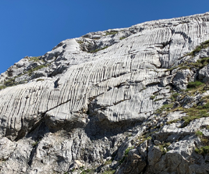
Linear karren patterns are dissolution features adorning the bare, inclined faces of soluble rocks, e.g. limestone (figure 1a). They appear as regularly spaced grooves following the incline and their hydrodynamical origin is undisputed (Ford & Williams Reference Ford and Williams2007; Ginés et al. Reference Ginés, Knez, Slabe and Dreybrodt2009). In contrast to fracture-induced forms, these grooves are caused by flows of rainwater or snow melt over the exposed rock surfaces. Their streamwise length as well as their transverse periodicity – observed in nature to span over length scales from millimetres to metres – are questions of particular interest, as they may shed light on past climatic conditions.

Figure 1. (a) Natural karren in the Bernese Alps (top) and in the Jura (bottom). (b) Sketch of the problem at hand.
Recent laboratory experiments by Guérin et al. (Reference Guérin, Derr, Courrech du Pont and Berhanu2020) showed that a uniform film flow carves an array of parallel rills on its gypsum substrate. Although the film thicknesses they probed were larger than in natural conditions and the flows presented wall-induced turbulence, this evidence highlighted the theoretical lack in the study of karren formation.
Bertagni & Camporeale (Reference Bertagni and Camporeale2021) provided the first theoretical analysis in the framework of linear stability theory. They used a complete description of the laminar hydrodynamical flow and, crucially, addressed the dissolution process by fully resolving the solute transport within the flow. They demonstrated the system's linear instability to transverse perturbations over a substantial range of wavenumbers and revealed the importance of transverse diffusion, both of momentum and solute, for the stabilisation of larger wavenumbers.
Here, we propose a boundary-layer approach to this linear karren instability. We consider a creeping, gravity-driven, streamwise-invariant flow. We model the dissolution process, by the use of Lévêque's (Reference Lévêque1928) boundary-layer solution, which profoundly simplifies the solute transport problem and enables us, together with the solution to the linearised Stokes equations, established by Bertagni & Camporeale (Reference Bertagni and Camporeale2021), to write a dispersion relation in closed form. The latter is remarkably faithful to the complete, tridimensional treatment of the solute transport by Bertagni & Camporeale (Reference Bertagni and Camporeale2021).
Finally, we propose to reduce the hydrodynamical description using two extended lubrication models, found in the literature. The revised lubrication theory, recently proposed by Devauchelle, Popović & Lajeunesse (Reference Devauchelle, Popović and Lajeunesse2022), may lack ‘the mathematical rigour of an order expansion’, notably as it includes the transverse momentum diffusion, while neglecting other effects, a priori of the same asymptotical weight, but is a very intuitive depth-integrated model. The weighted-residual integral boundary-layer methodology (see Kalliadasis et al. (Reference Kalliadasis, Ruyer-Quil, Sheid and Velarde2012) and references therein), on the other hand, has the advantage of being asymptotically consistent, although somewhat tedious to manipulate. Both produce sets of depth-integrated streamwise and transverse momentum conservation equations, which further emphasise the simple underlying physics of the coupling in the problem at hand: the streamwise component of the flow interacts with the dissolution process, while the transverse flow serves to flatten the free surface. Their results are validated against the exact linearised Stokes equations.
2. Problem formulation and modelisation
We investigate the laminar, incompressible, gravity-driven flow of a thin film of Newtonian liquid (water) of density  $\rho$, kinematic viscosity $\nu$ and surface tension $\sigma$ over a soluble substrate (e.g. limestone or gypsum), inclined by an angle $\theta$ with respect to the horizontal, and the solute transport inside the film, with diffusion coefficient $D$ (figure 1b). The substrate material's insolubility $\gamma =\rho _s/c_{sat}$ is defined as a dimensionless solid density ratio between its crystallised and dissolved states, where $\rho _s$ is the rock's density and $c_{sat}$ is the equilibrium, i.e. saturated, mass concentration in the liquid.
2.1. Governing equations
The system is governed by the continuity, the Stokes and the advection–diffusion equations. We make the problem dimensionless by rescaling all lengths by the characteristic film thickness  $H_N$, the pressure p by a hydrostatic pressure scale $\rho g\sin \theta H_N/2$ and the velocity ${\boldsymbol{u}}$ by a Nusselt velocity scale $g \sin \theta H_N^2/(2\nu )$, where g is the gravitational acceleration. Lastly, we rescale the concentration c by its saturated value $c_{sat}$. Assuming that the concentration field adapts instantly to the flow, i.e. in a quasi-stationary regime, the governing equations read
 \begin{gather} \boldsymbol{\nabla}\boldsymbol{\cdot} \boldsymbol{u}=0, \end{gather}
 \begin{gather}\boldsymbol{\nabla}p=\nabla^2\boldsymbol{u}+\boldsymbol{f}, \end{gather}
 \begin{gather}{Pe} \boldsymbol{u}\boldsymbol{\cdot} \boldsymbol{\nabla} c=\nabla^2 c, \end{gather}
where  $\boldsymbol {f}=2\hat {\boldsymbol {x}}-2\cot \theta \hat {\boldsymbol {y}}$ is the gravity forcing. The Péclet number ${Pe}=g\sin \theta H_N^3/(2 \nu D)$ is the product of the Reynolds and Schmidt numbers ${Sc}=\nu /D=10^3$, and can therefore be large even for creeping flows.
As the considered water films are usually formed by rainwater runoff or snow melt, the water is assumed solute-free at the inlet:
 \begin{equation} c|_{x=0}=0. \end{equation}
In general, the dissolution process is governed by a competition between the surface reaction and diffusion rates. For simple dissolution reactions, the comparison is relatively straightforward: the dissolution of very soluble minerals, e.g. salt, are overwhelmingly diffusion-controlled. In contrast, the dissolution of calcite involves a much more sophisticated chemical reaction, the kinetics of which can vary substantially with the conditions. It is usually accepted that calcite's dissolution in very undersaturated water is also transport-controlled (Ford & Williams Reference Ford and Williams2007). This means that the reaction at the solid–liquid interface is quasi-instantaneous; the water is nearly saturated at contact with the rock,
 \begin{equation} c|_{y=\eta}=1, \end{equation}
and the dissolution rate is thus regulated by how fast diffusion can evacuate the solute. The solid mass conservation equation then governs the geomorphological evolution:
 \begin{equation} \gamma {Pe} \partial_t \eta=\boldsymbol{\nabla}c\boldsymbol{\cdot} \boldsymbol{\nabla}[y-\eta]|_{y=\eta}. \end{equation}
We remind the reader that the dimensionless parameter  $\gamma$ measures the insolubility of the substrate material; it is large for weakly soluble materials, e.g. $\gamma =49\ 091$ for calcite (Bertagni & Camporeale Reference Bertagni and Camporeale2021). Moreover, there is no solute flux through the liquid–air interface
 \begin{equation} \boldsymbol{\nabla}c\boldsymbol{\cdot} \boldsymbol{\nabla}[y-\eta-h]|_{y=\eta+h}=0. \end{equation}
 From (2.4c), we observe that the geomorphological time scale is much larger than the hydrodynamical one. The substrate's evolution – being controlled by diffusion,  ${Pe}\gg 1$, and undergoing a dramatic reduction in its solid density, $\gamma \gg 1$ – is vastly slower than the flow velocities, which enables us to use the classical no-slip and no-penetration boundary conditions at the substrate:
 \begin{equation} \boldsymbol{u}|_{y=\eta}=\boldsymbol{0}. \end{equation}
The kinematic boundary condition describes the evolution of the film's thickness:
 \begin{equation} \partial_t h = \boldsymbol{u}\boldsymbol{\cdot} \boldsymbol{\nabla}[y-\eta-h]|_{y=\eta+h}. \end{equation}
Finally, the liquid–air interface is free of tangential stresses and undergoing a capillary jump in the normal stress:
 \begin{equation} {\boldsymbol{\mathsf{T}}}\boldsymbol{\cdot} \boldsymbol{\nabla}[y-\eta-h]|_{y=\eta+h} ={-}{We} {\mathcal{K}} \boldsymbol{\nabla}[y-\eta-h], \end{equation}
with the stress tensor  ${\boldsymbol{\mathsf{T}}}=-p{\boldsymbol{\mathsf{I}}}+(\boldsymbol {\nabla } \boldsymbol {u}+\boldsymbol {\nabla } \boldsymbol {u}^T)$, the curvature
 \begin{equation} {\mathcal{K}}=\boldsymbol{\nabla}\boldsymbol{\cdot} \left[\frac{\boldsymbol{\nabla}[y-\eta-h]}{\|\boldsymbol{\nabla}[y-\eta-h]\|}\right], \end{equation}
and the Weber number  ${We}=2\sigma /(\rho g\sin \theta H_N^2)$. The gradient expressions $\boldsymbol {\nabla }[y-\eta -h]$ and $\boldsymbol {\nabla }[y-\eta ]$ are the upward-pointing vectors, normal to the upper and lower boundaries of the liquid domain, respectively. They are not normalised in the kinematic and dissolution conditions ((2.5b), (2.4c)), as $\partial _t h$ and $\partial _t\eta$ are themselves projections of the normal interface velocities onto $\hat {\boldsymbol {y}}$.
2.2. Flat-rock basic flow
The stationary, transverse-invariant basic flow is that of a uniform liquid film falling over an inclined flat rock,
 \begin{equation} h_b=1,\quad \eta_b=0, \end{equation}
involving a half-Poiseuille streamwise velocity profile and a hydrostatic pressure field
 \begin{equation} \boldsymbol{u_b}=y(2-y)\hat{\boldsymbol{x}},\quad p_b=2\cot\theta(1-y). \end{equation}
 Polyanin et al. (Reference Polyanin, Kutepov, Vyazmin and Kazenin2001, pp. 130–132) provide an exact solution to the advection–diffusion equation (2.3) for this basic flow, ignoring the streamwise diffusion  $(\partial _x^2 c_b)$, which is negligible for large Péclet numbers ${Pe}$ (figure 2). Near the inlet, the solute forms a thin boundary layer, outside of which the water remains pure. The thickness of this layer grows due to diffusion and the water's aggressivity towards the substrate decreases. Downstream, the accumulation of solute saturates the film.

Figure 2. Two-dimensional basic concentration field  $c_b$ and wall-normal profiles at $x/{Pe}=\{10^{-3}, 10^{-2}, 10^{-1}, 1\}$. The orange solid lines represent the exact solution, while the black dashed lines depict Lévêque's (Reference Lévêque1928) boundary-layer solution.
Since the basic concentration field and, crucially, its gradient at the substrate are a function of the streamwise coordinate  $x$, flat rock cannot be an exact solution. Bertagni & Camporeale (Reference Bertagni and Camporeale2021) remedied this by isolating the dissolution rate induced by the uniform film flow $V$ from the evolution of the substrate $\partial _t\eta$. They formulated the dissolution law (2.4c) as
 \begin{equation} \gamma {Pe}(\partial_t \eta-V)=\boldsymbol{\nabla}c\boldsymbol{\cdot} \boldsymbol{\nabla}[y-\eta]|_{y=\eta},\quad \text{with }\gamma {Pe} V={-}\partial_y c_b|_{y=0}. \end{equation}
2.3. Solutal Lévêque boundary-layer dissolution model
Let us focus on the region near the inlet, where the water is almost pure of solute. The concentration interacts with the velocity field only very close to the wall, in a solutal boundary layer, where the velocity has an almost purely shear profile. Under these conditions,  $x\ll {Pe}$, and keeping only the streamwise advection and the wall-normal diffusion, Lévêque (Reference Lévêque1928) reduced the advection–diffusion equation (2.3) to
 \begin{equation} {Pe} \tau (y-\eta)\partial_x c=\partial_y^2c, \end{equation}
where the advecting streamwise velocity is asymptotically expanded using its shear rate at the substrate  $\tau =\partial _y u|_{y=\eta }$, and subject to boundary conditions
 \begin{equation} c|_{x=0}=0, \quad c|_{y=\eta}=1, \quad \partial_y c|_{y\to\infty}=0. \end{equation}
Lévêque (Reference Lévêque1928) obtained a self-similar solution, which reads
 \begin{equation} c(x,y)=\frac{\varGamma\left(\dfrac{1}{3},\dfrac{{Pe} \tau (y-\eta)^3}{9 x}\right)}{\varGamma(1/3)},\end{equation}
with  $\varGamma (a,s)=\int _s^\infty t^{a-1}\,\mathrm {e}^{-t}\,\mathrm {d}t$ and $\varGamma (a)\equiv \varGamma (a, 0)$ – the incomplete and complete gamma functions, respectively. For the basic flow, $\tau _b=2$ and $\eta _b=0$, this solution is compared to the exact one in figure 2 and is found to be fairly valid up to $x/{Pe}\lesssim 0.1$, as already noted by Bertagni & Camporeale (Reference Bertagni and Camporeale2021).
By injecting this solution (2.11) into the dissolution law (2.8), we obtain the following evolution equation:
 \begin{equation} \partial_t\eta=V-(\gamma{Pe})^{{-}1}\|\boldsymbol{\nabla}[y -\eta]\|^2 \partial_y c|_{y=\eta}=V (1-\|\boldsymbol{\nabla}[y-\eta]\|^2(\tau/\tau_b)^{1/3}), \end{equation}
with  $V=(6{Pe}/x)^{1/3}/(\gamma {Pe}\varGamma (1/3))$ and where we have used the saturation condition (2.4b) to rewrite $\boldsymbol {\nabla }c\boldsymbol {\cdot } \boldsymbol {\nabla }[y-\eta ]|_{y=\eta }=\|\boldsymbol {\nabla }[y-\eta ]\|^2\partial _y c|_{y=\eta }$. This model indeed ignores the in-plane concentration diffusion, which is important at small wavelengths, but should capture well the behaviour of the boundary layer's thickness with respect to the streamwise velocity.
2.4. Depth-integrated hydrodynamical models
At this stage, only the streamwise shear rate at the rock surface  $\tau$ is necessary for closing the problem with the dissolution model (2.12). As mentioned above, Bertagni & Camporeale (Reference Bertagni and Camporeale2021) achieved an exact solution to the linearised Stokes equations for this problem, which can be directly applied here for the purposes of linear stability analysis, as we will see in § 3.1. However, with the purpose to validate fully depth-averaged models, we set out to generalise two extended lubrication methodologies and obtain three closed-form expressions for the dispersion relation. We believe that depth-averaged models could in future prove very useful when it comes to studying the nonlinear evolution of linear karren patterns. They can suitably be used as surrogates for the full Stokes equations with a free interface, which would require an interface-capturing or interface-tracking multiphase solver. A Wolfram Mathematica script, performing the mathematical derivations from this section, is available as supplementary material at https://doi.org/10.1017/jfm.2023.932.
2.4.1. Revised lubrication model
Firstly, following Devauchelle et al. (Reference Devauchelle, Popović and Lajeunesse2022), and generalising their model to free-surface flows, we make a half-Poiseuille ansatz for the in-plane velocity profiles,
 \begin{equation} u(y,z)\hat{\boldsymbol{x}}+w(y,z)\hat{\boldsymbol{z}} =\frac{3\boldsymbol{q}(z)}{h(z)}F_0\left[\frac{y-\eta(z)}{h(z)}\right], \end{equation}
with the local flow rate vector  $\boldsymbol {q}=q_x\hat {\boldsymbol {x}}+q_z\hat {\boldsymbol {z}}$. The $y$-dependence of the in-plane velocity field is isolated into a semi-parabolic structure
 \begin{equation} F_0[\zeta ]=\zeta -\zeta ^2/2, \end{equation}
ensuring the no-slip condition (2.5a) on the wall and a leading-order, long-wave version of the stress-free dynamic boundary condition (2.5c) on the water–air interface ( $\partial _y u|_{y=\eta +h}=\partial _y w|_{y=\eta +h}=0$). The mass conservation equation reads
 \begin{equation} \partial_t h+q_z'=0, \end{equation}
where the prime  $'$ denotes a differentiation with respect to $z$.
$z$.
The integration of the wall-normal component of the momentum equations (2.2) produces the hydrostatic pressure field
 \begin{equation} p(y,z)=2\cot\theta(\eta+h-y)+{We}{\mathcal{K}}, \end{equation}
which includes the capillary contribution of the curved interface and where, in the lubrication spirit, we have ignored the wall-normal momentum's diffusion  $\nabla ^2 v$.
Finally, using the ansatz (2.13), we integrate the in-plane components of the Stokes equations (2.2) through the film and obtain the following momentum conservation equations:
 \begin{align}
\left(1+\eta'^2-h'\eta'-h'^2+\frac{h(h''+\eta'')}{2}\right)
\boldsymbol{q} & +h(h'+\eta')\boldsymbol{q}'-\frac{h^2\boldsymbol{q}''}{3} \nonumber\\
& =\dfrac{h^3}{3}(2\hat{\boldsymbol{x}}-2\cot
\theta(h'+\eta')\hat{\boldsymbol{z}}-{We}{\mathcal{K}}'\hat{\boldsymbol{z}}).
\end{align}
\begin{align}
\left(1+\eta'^2-h'\eta'-h'^2+\frac{h(h''+\eta'')}{2}\right)
\boldsymbol{q} & +h(h'+\eta')\boldsymbol{q}'-\frac{h^2\boldsymbol{q}''}{3} \nonumber\\
& =\dfrac{h^3}{3}(2\hat{\boldsymbol{x}}-2\cot
\theta(h'+\eta')\hat{\boldsymbol{z}}-{We}{\mathcal{K}}'\hat{\boldsymbol{z}}).
\end{align}There are three sources of depth-integrated momentum: the streamwise projection of the gravitational acceleration and the transverse hydrostatic and capillary pressure gradients, generated by deformations of the free surface.
The revision, proposed by Devauchelle et al. (Reference Devauchelle, Popović and Lajeunesse2022), essentially consists in allowing  $\boldsymbol {q}$ to keep an autonomous dependence on $z$, instead of it being adiabatically slaved to $h$ and $\eta$, as in the classical lubrication theory (Kalliadasis et al. Reference Kalliadasis, Ruyer-Quil, Sheid and Velarde2012), where
 \begin{equation} \boldsymbol{q}=\frac{h^3}{3}(2\hat{\boldsymbol{x}} -2\cot\theta(h'+\eta')\hat{\boldsymbol{z}}-{We}{\mathcal{K}}'\hat{\boldsymbol{z}}). \end{equation}
Evaluating the streamwise shear rate at the substrate from the ansatz (2.13) produces
 \begin{equation} \tau=\frac{3 q_x}{h^2}. \end{equation}
2.4.2. Weighted-residual integral boundary-layer model
Secondly, following the derivations gathered in the monograph of Kalliadasis et al. (Reference Kalliadasis, Ruyer-Quil, Sheid and Velarde2012), we aim at a weighted-residuals formulation for the free-surface thin-film flow over a variable substrate morphology  $\eta (z)$. We rewrite the Stokes equations (2.2) as a set of streamwise-invariant boundary-layer equations, which are asymptotically consistent up to second order (so as to keep the in-plane momentum diffusion) in a thin-film order parameter, separating in-plane and wall-normal length scales,
 \begin{gather} 2+\partial_y^2 u+\partial_z^2u=0, \end{gather}
 \begin{gather}-2\cot\theta-\partial_y p+\partial_y^2 v=0, \end{gather}
 \begin{gather}-\partial_z p+\partial_y^2 w+\partial_z^2 w=0, \end{gather}
with the dynamic boundary conditions now reading
 \begin{gather} \partial_y u|_{y=h+\eta}=\partial_z[h+\eta] \partial_z u|_{y=h+\eta}, \end{gather}
 \begin{gather}\partial_y w|_{y=h+\eta}=4\partial_z[h+\eta] \partial_z w|_{y=h+\eta}-\partial_z v|_{y=h+\eta}, \end{gather}
 \begin{gather}p|_{y=h+\eta}=2\partial_y v|_{y=h+\eta}-{We}\partial_z^2[h+\eta]. \end{gather}
 In order to account for higher-order deviations from the half-Poiseuille profile, the in-plane velocity ansatz is corrected with two additional polynomial functions, weighted by their associated coefficients  $\boldsymbol {r}=r_x\hat {\boldsymbol {x}}+r_z\hat {\boldsymbol {z}}$ and $\boldsymbol {s}=s_x\hat {\boldsymbol {x}}+s_z\hat {\boldsymbol {z}}$:
 \begin{equation} u(y,z)\hat{\boldsymbol{x}}+w(y,z)\hat{\boldsymbol{z}}= \frac{3(\boldsymbol{q}-\boldsymbol{r}-\boldsymbol{s})}{h}F_0 \left[\frac{y-\eta}{h}\right]+\frac{45 \boldsymbol{r}}{h}F_1\left[\frac{y-\eta}{h}\right]+\frac{210 \boldsymbol{s}}{h}F_2\left[\frac{y-\eta}{h}\right], \end{equation}
where
 \begin{align}
F_1[\zeta]&=\zeta-\frac{17\zeta^2}{6}+\frac{7\zeta^3}{3}-\frac{7\zeta^4}{12},\nonumber\\
F_2[\zeta]&=\zeta-\frac{13\zeta^2}{2}+\frac{57\zeta^3}{4}-
\frac{111\zeta^4}{8}+\frac{99\zeta^5}{16}-\frac{33\zeta^6}{32},
\end{align}
\begin{align}
F_1[\zeta]&=\zeta-\frac{17\zeta^2}{6}+\frac{7\zeta^3}{3}-\frac{7\zeta^4}{12},\nonumber\\
F_2[\zeta]&=\zeta-\frac{13\zeta^2}{2}+\frac{57\zeta^3}{4}-
\frac{111\zeta^4}{8}+\frac{99\zeta^5}{16}-\frac{33\zeta^6}{32},
\end{align}
which are chosen orthogonal to one another, and to  $F_0[\zeta ]$, with respect to the scalar product $\langle a|b\rangle =\int _\eta ^{h+\eta } a b\,\mathrm {d} y$, and satisfy the leading-order boundary conditions. The local flow rate vector remains $\boldsymbol {q}$ and hence the mass conservation equation (2.15) still holds. The corrections $\boldsymbol {r}$ and $\boldsymbol {s}$ are at least of order 1 in the thin-film parameter, so that their second derivatives with respect to $z$ fall out of the boundary-layer equations (2.20). Since their first derivatives do not appear in the equations either, $\boldsymbol {r}$ and $\boldsymbol {s}$ are adiabatically slaved to $\boldsymbol {q}$, $h$ and $\eta$.
The pressure field is integrated from the wall-normal boundary-layer equation (2.20b):
 \begin{equation} p=2\cot\theta(h+\eta-y)-\partial_z w -\partial_z w|_{y=h+\eta}-{We}(h''+\eta''), \end{equation}
where we have used the continuity equation (2.1) to replace  $\partial _y v$.
Finally, we perform a Galerkin projection of the in-plane boundary-layer momentum equations (2.17) onto the basis functions themselves,
 \begin{gather} \left\langle \left.F_i\left[\frac{y-\eta}{h}\right]\right|2 +\partial_z^2u\right\rangle+F_i[1]\partial_y u|_{y=h+\eta} +\left\langle \partial_y^2F_i \left. \left[\dfrac{y-\eta}{h}\right]\right|u\right\rangle=0, \end{gather}
 \begin{gather}\left\langle \left.F_i\left[\frac{y-\eta}{h}\right]\right| -\partial_z p+\partial_z^2 w\right\rangle+F_i[1] \partial_y w|_{y=h+\eta}+\left\langle \partial_y^2F_i \left.\left[\frac{y-\eta}{h}\right]\right|w\right\rangle=0 \end{gather}
with  $i=\{0,1,2\}$, and where we have integrated by parts the wall-normal diffusion terms in order to introduce explicitly the second-order dynamic boundary conditions (2.21a,b). The projections onto $F_0$ readily produce the following momentum conservation equations:
 \begin{equation}
\left(1+\eta'^2+\frac{h'\eta'}{2}-\frac{3h'^2}{10}+
\frac{h(23h''+15\eta'')}{40}\right)q_x+\frac{2h h'
q_x'}{5}- \frac{2h^2q_x''}{5}=\frac{2h^3}{3},
\end{equation}
\begin{equation}
\left(1+\eta'^2+\frac{h'\eta'}{2}-\frac{3h'^2}{10}+
\frac{h(23h''+15\eta'')}{40}\right)q_x+\frac{2h h'
q_x'}{5}- \frac{2h^2q_x''}{5}=\frac{2h^3}{3},
\end{equation} \begin{align}
\left(1+2\eta'^2+h'\eta'-\frac{8h'^2}{5}+\frac{h(24h''
+15\eta'')}{10}\right)q_z&+\frac{9h h' q_z'}{5}-
\frac{9h^2q_z''}{5} \nonumber\\
& =\dfrac{h^3}{3}({-}2\cot\theta(h'+\eta')+{We}(h'''+\eta''')),
\end{align}
\begin{align}
\left(1+2\eta'^2+h'\eta'-\frac{8h'^2}{5}+\frac{h(24h''
+15\eta'')}{10}\right)q_z&+\frac{9h h' q_z'}{5}-
\frac{9h^2q_z''}{5} \nonumber\\
& =\dfrac{h^3}{3}({-}2\cot\theta(h'+\eta')+{We}(h'''+\eta''')),
\end{align}
while the corrections  $\boldsymbol {r}$ and $\boldsymbol {s}$ can be computed from the other residual equations $i=\{1,2\}$.
The streamwise shear rate is then obtained from the corrected ansatz (2.22):
 \begin{equation} \tau=\left(1+\frac{51h'\eta'}{64}-\frac{h'^2}{320}+ \frac{h(53h''-75\eta'')}{640}\right)\frac{3q_x}{h^2}+ \frac{69h'-315\eta'}{320}\frac{q_x'}{h}-\frac{q_x''}{5}. \end{equation}
3. Linear stability analysis
3.1. Linearised Stokes equations
As mentioned in § 2.4, Bertagni & Camporeale (Reference Bertagni and Camporeale2021) provide an exact solution in closed form to the hydrodynamical problem ((2.1), (2.2)), linearised around the basic flow (2.7c,d), with boundary conditions (2.6c,d), linearised and flattened around the flat-rock solution (2.7a,b). Thanks to the streamwise invariance, the continuity equation enables them to write the cross-stream components of the perturbation velocity field in terms of a scalar streamfunction  $\varphi$, separate from the streamwise perturbation velocity. After a normal mode decomposition
 \begin{equation} (\boldsymbol{u};h,\eta)=(\boldsymbol{u}_b;1,0) +\epsilon(\tilde{u}(y)\hat{\boldsymbol{x}}-\mathrm{i} k\tilde{\varphi}(y)\hat{\boldsymbol{y}}+\partial_y \tilde{\varphi}(y)\hat{\boldsymbol{z}};\tilde{h}, \tilde{\eta})\exp[\mathrm{i}(k z-\omega t)]+\textrm{c.c.}, \end{equation}
with real transverse wavenumber  $k$ and angular frequency $\omega$, the imaginary part of which is the temporal growth rate, their solution reads in the present notation
 \begin{equation} \left.\begin{array}{@{}l@{}}
\tilde{u}=2\operatorname{sech} k
\left((\tilde{h}+\tilde{\eta})\dfrac{\sinh[k
y]}{k}-\tilde{\eta}\cosh[k-k y]\right),\\
\tilde{\varphi}=\mathrm{i}(2\cot\theta+{We} k^2) \\
\qquad \times\dfrac{(k y\coth[k y]-1)(k\sinh k+\cosh k)-k^2 y\cosh
k}{k^2(2k^2+\cosh[2k]+1)} \sinh[k
y](\tilde{h}+\tilde{\eta}).
\end{array}\right\}
\end{equation}
\begin{equation} \left.\begin{array}{@{}l@{}}
\tilde{u}=2\operatorname{sech} k
\left((\tilde{h}+\tilde{\eta})\dfrac{\sinh[k
y]}{k}-\tilde{\eta}\cosh[k-k y]\right),\\
\tilde{\varphi}=\mathrm{i}(2\cot\theta+{We} k^2) \\
\qquad \times\dfrac{(k y\coth[k y]-1)(k\sinh k+\cosh k)-k^2 y\cosh
k}{k^2(2k^2+\cosh[2k]+1)} \sinh[k
y](\tilde{h}+\tilde{\eta}).
\end{array}\right\}
\end{equation}The linearised and flattened kinematic boundary condition and dissolution model ((2.5b), (2.12)) can then form the system of solvability equations
 \begin{gather} \omega \tilde{h}=k\tilde{\varphi}|_{y=1}, \end{gather}
 \begin{gather}\mathrm{i}\omega \tilde{\eta}=\dfrac{V}{6} (\partial_y \tilde{u}|_{y=0}+\tilde{\eta}\partial_y^2 u_b|_{y=0}), \end{gather}
which is singular and hence allows for non-trivial solutions when
 \begin{equation} \omega_\pm^{lS}(k)=\dfrac{\omega_0^{lS}}{2}\pm \sqrt{\left(\dfrac{\omega_0^{lS}}{2}\right)^2-\dfrac{V(\cosh k\sinh k-k)(1-k\tanh k)}{3k(2 k^2+\cosh[2k]+1)}(2\cot\theta+{We} k^2)},\end{equation}
with
 \begin{equation} \omega_0^{lS}={-}\mathrm{i}\left\{\dfrac{\cosh k\sinh k-k}{k(2 k^2+\cosh[2k]+1)}(2\cot\theta+{We} k^2)+\dfrac{V}{3}(\operatorname{sech} k+k\tanh k-1)\right\}. \end{equation}
3.2. Linearised depth-integrated models
The two depth-integrated models, developed in § 2.4 to replace the Stokes equations, instead reduce the problem to four scalar variables  $(q_x,q_z;h,\eta )$, governed by four equations ((2.17) or (2.26), (2.15), and (2.12) with either (2.19) or (2.27)). The perturbed state is expressed in the form
 \begin{equation} (q_x,q_z;h,\eta)=(2/3,0;1,0)+\epsilon (\tilde{q}_x,\tilde{q}_z;\tilde{h},\tilde{\eta}) \exp[\mathrm{i}(k z-\omega t)]+ \textrm{c.c.} \end{equation}
For the revised lubrication model, presented in § 2.4.1, the linearised perturbation evolution equations then read
 \begin{gather} (3+k^2)\tilde{q}_x-(6+k^2)\tilde{h}-k^2\tilde{\eta}=0, \end{gather}
 \begin{gather}(3+k^2)\tilde{q}_z+\mathrm{i}k(2\cot\theta+{We} k^2) (\tilde{h}+\tilde{\eta})=0, \end{gather}
 \begin{gather}k \tilde{q}_z-\omega\tilde{h}=0, \end{gather}
 \begin{gather}V(3\tilde{q}_x/2-2\tilde{h})-3\mathrm{i}\omega\tilde{\eta}=0. \end{gather}
We obtain the following dispersion relation:
 \begin{equation} \omega_\pm^{rl}(k)=\dfrac{\omega_0^{rl}}{2}\pm \sqrt{\left(\dfrac{\omega_0^{rl}}{2}\right)^2- \dfrac{V k^2 (1-2 k^2/3)}{(3+k^2)^2}(2\cot\theta+{We} k^2)}, \end{equation}
with  $\omega _0^{rl}=-\mathrm {i}k^2(2\cot \theta +{We} k^2+V/2)/(3+k^2)$.
For the weighted-residuals model, presented in § 2.4.2, the linearised perturbation evolution equations instead read
 \begin{gather} (3+6k^2/5)\tilde{q}_x-(6+23k^2/20)\tilde{h}-3k^2\tilde{\eta}/4=0, \end{gather}
 \begin{gather}(3+27k^2/5)\tilde{q}_z+\mathrm{i}k(2\cot\theta+{We} k^2) (\tilde{h}+\tilde{\eta})=0, \end{gather}
 \begin{gather}k \tilde{q}_z-\omega\tilde{h}=0, \end{gather}
 \begin{gather}V(5\tilde{q}_x/4-(3/2-5k^2/384)\tilde{h}+23 k^2\tilde{\eta}/128) -3\mathrm{i}\omega\tilde{\eta}=0. \end{gather}
The dispersion relation becomes
 \begin{equation} \omega_\pm^{wr}(k)=\dfrac{\omega_0^{wr}}{2}\pm \sqrt{\left(\dfrac{\omega_0^{wr}}{2}\right)^2-\dfrac{V k^2 (1-k^2(9+k^2)/15)}{(3+6k^2/5)(3+27k^2/5)}\left(2\cot\theta+{We} k^2\right)}, \end{equation}
with
 \begin{equation} \omega_0^{wr}={-}\mathrm{i}k^2\left\{\dfrac{2\cot\theta+{We} k^2}{3+27k^2/5} +\dfrac{21V(1+46k^2/315)}{128+256k^2/5}\right\}. \end{equation}
3.3. Results
Figure 3 presents these dispersion relations ((3.4), (3.8), (3.10)) for different inclination angles  $\theta$. In the presented range, the weighted-residuals dispersion relation is visually indistinguishable from the linear Stokes one. Both gravity and surface tension are destabilising at small $k$. The instability is neutralised linearly when $k\to 0$ for $\theta \ne {\rm \pi}/2$ and quadratically for a vertical substrate. Larger wavenumbers, $k\tanh k>1\Leftrightarrow k^2>1.439$ for the linear Stokes model, $k^2>3/2$ for the revised lubrication model, or $k^2>(\sqrt {141}-9)/2\approx 1.437$ for the weighted-residuals model, are stabilised by the transverse transfer of momentum, emulated strikingly well by the diffusion terms in the two extended lubrication models ((2.17), (2.26)).

Figure 3. Dispersion relations ((3.4), (3.8), (3.10)) compared to Bertagni & Camporeale (Reference Bertagni and Camporeale2021). Here  ${Pe}=10^3$, $\gamma =49\ 091$ (calcite), $x=10$, $\theta =\{{\rm \pi} /8, {\rm \pi}/4, 3{\rm \pi} /8, {\rm \pi}/2\}$, ${We}\approx 4210\times \sin ^{-1/3}\theta$.
These simplified models appear to capture in a distilled form most of the necessary physics to compare rather favourably with the much more involved and complete analytical treatment of Bertagni & Camporeale (Reference Bertagni and Camporeale2021). Deviations are observed only for the cutoff wavenumber, which can be accounted for by the lack of transverse solute diffusion in Lévêque's (Reference Lévêque1928) boundary-layer dissolution model (see their figure 5c).
In the spirit of Bertagni & Camporeale (Reference Bertagni and Camporeale2021), figure 4(a) illustrates the influence of the Péclet number  ${Pe}$ on the dispersion relation (3.4). Our analysis retrieves a behaviour rather faithful to what they report. We remind the reader that ${Pe}={Sc}{Re}$ with the Schmidt number ${Sc}=\nu /D$. Figure 4(b) shows the dispersion relation for different materials, to be compared again with the results of Bertagni & Camporeale (Reference Bertagni and Camporeale2021). More soluble minerals, e.g. salt, exhibit a shorter plateau of larger growth rate.

Figure 4. (a) Contour plot of the growth rate  ${\textrm {Im}}[\omega _+]$ (3.4) in the { $k$,
$k$,  ${Pe}$} space. The most unstable wavenumber $k_m$ is displayed by a dashed line. The striped area indicates negative growth rates. Here $\gamma =49\ 091$ (calcite), $x/{Pe}=0.05$, $\theta ={\rm \pi} /4$, ${We}\approx 4.7\times 10^5\times {Pe}^{-2/3}$. (b) Dispersion relation (3.4) for several materials. Here ${Pe}=10^3$, $x=10$, $\theta ={\rm \pi} /4$, ${We}\approx 4726$.
3.4. Instability mechanism
We briefly elucidate here the instability mechanism, explained by Guérin et al. (Reference Guérin, Derr, Courrech du Pont and Berhanu2020) and depicted in figure 7 of Bertagni & Camporeale (Reference Bertagni and Camporeale2021). Let the substrate be perturbed by a sinusoidal wave in the transverse direction  $z$. Then, over the troughs (i) the film gets thicker – on the one hand because of a hydrostatic pressure gradient, which tends to bring water back down in the troughs, and on the other hand because of a capillary pressure gradient, which tends to keep the free surface flat; (ii) the flow accelerates; (iii) the boundary layer becomes thinner; and (iv) the dissolution is faster than on the crests.
For shorter wavelengths, transverse transfer of momentum becomes important and the flow acceleration in step (ii) is hindered. Inside the narrower troughs the flow is confined and in fact slowed down, thus stabilising the system.
For very long wavelengths, the flattening of the free surface, step (i), becomes a growth-limiting factor and the instability is neutralised. This explains the qualitatively different asymptotic behaviour of the growth rate for  $\theta ={\rm \pi} /2$: without a wall-normal component of the gravitational acceleration, surface tension is the only effect restoring the flat free surface. This is also why in the rigid-lid approximation, where $\tilde {h}+\tilde {\eta }=0$ is imposed, bypassing step (i) altogether, the unstable plateau reaches $k=0$, as highlighted by Bertagni & Camporeale (Reference Bertagni and Camporeale2021).
4. Conclusion
The dispersion relation displays a large plateau of almost equally unstable wavenumbers in the interval  $10^{-3}\lesssim k\lesssim 10^{-1}$ (figure 3). This impedes to some degree the model's predictive power, since a large range of wavelengths – spanning from ten to approximately a thousand times the film thickness $H_N$ – can grow with very similar rates. On the other hand, this feature may be consistent with the wide-ranging length scales spanned by natural linear karren forms. The competition for the emerging pattern's ultimate wavelength would be settled by more subtle mechanisms. Finite amplitude and stochastic effects, such as the roughness and/or grain distribution of the initial rock surface, or raindrop impacts on the falling film, might play a role in the wavelength selection.
It is clear that the classical lubrication theory could not predict a cutoff wavenumber – while the film is thicker over the troughs, the flow would always be faster, and the troughs would dissolve more, independent of  $k$. In this sense, both extended lubrication models, because they account for the transverse transfer of momentum, have proven to be suitable. Moreover, their striking adjacency underlines the place of physical insight in simplifying mathematically cumbersome systems. Finally, their validation against the exact Stokes equations, at least in the linear regime, holds a promise for their future use in nonlinear analyses.
Supplementary material
Supplementary material are available at https://doi.org/10.1017/jfm.2023.932.
Acknowledgements
The authors are grateful to T. Salamon and M. Chaigne for fruitful discussions.
Declaration of interests
The authors report no conflict of interest.


 Open access