


1. Introduction
The aggregation of cohesive particles in turbulence depends on such quantities as particle size, density and volume fraction, as well as on the cohesive force strength and the turbulent shear rate. Experimental studies have provided substantial insight into key aspects of the flocculation process, although the role of the shear rate remains somewhat controversial. The pioneering work by Winterwerp (Reference Winterwerp1998) found that the equilibrium floc size  $D_{f,eq}$ scales inversely with the turbulent shear rate $G$, viz. $D_{f,eq} \sim G^{-0.5}$. Most subsequent experiments confirmed that $D_{f,eq}$ decreases for larger $G$ (Spicer et al. Reference Spicer, Pratsinis, Raper, Amal, Bushell and Meesters1998; Soos et al. Reference Soos, Moussa, Ehrl, Sefcik, Wu and Morbidelli2008; Bubakova, Pivokonsky & Filip Reference Bubakova, Pivokonsky and Filip2013; Zhang et al. Reference Zhang, Yang, Zang, Cheng and Zhang2019). On the other hand, several authors observed the opposite trend of larger flocs for stronger shear in flows with low shear (He et al. Reference He, Nan, Li and Li2012; Wang et al. Reference Wang, Nan, Ji and Yang2018). Dyer (Reference Dyer1989) introduced the concept of a maximum floc size at intermediate shear, while emphasizing the need for further investigation. Serra, Colomer & Logan (Reference Serra, Colomer and Logan2008) speculated that for low-shear flows the preferential concentration of sediment by turbulence dominates over the breakage of aggregates, so that stronger shear promotes larger flocs. Mietta et al. (Reference Mietta, Chassagne, Manning and Winterwerp2009) discussed the role of experimental error, and they argued that it is difficult to keep particles suspended in low-shear flow due to settling, so that the flocculation process may be incomplete in experimental devices with limited depth.
The current investigation aims to shed light on the above issues by employing particle-resolving numerical simulations that can capture the interplay of hydrodynamic, inertial and inter-particle forces during the growth, deformation and breakup of flocs. In the spirit of earlier investigations by Maxey (Reference Maxey1987), Bergougnoux et al. (Reference Bergougnoux, Bouchet, Lopez and Guazzelli2014) and Zhao et al. (Reference Zhao, Vowinckel, Hsu, Köllner, Bai and Meiburg2020), we will employ one-way coupled simulations of two-dimensional, steady, spatially periodic Taylor–Green vortices (with fluid density  $\rho _f$ and dynamic viscosity $\mu$), cf. figure 1(a). For a few select parameter combinations we will compare the one-way coupled results with two-way coupled simulations. The shear rate and Reynolds number associated with this flow are $G = U/\eta$ and $Re = \eta U \rho _f/ \mu$, where $\eta$ and $U$ are the characteristic length and velocity scales of the cellular vortex flow, respectively. In order to investigate behaviour at viscous scales of turbulence, we fix $Re = 1$ which yields $\eta = \sqrt {\mu /(\rho _f G)}$ and $U = \sqrt {\mu G / \rho _f}$.

Figure 1. (a) Streamlines of the spatially periodic, two-dimensional cellular Taylor–Green vortex flow. (b) The relationship between the dimensionless particle size  $\tilde D_p$ and the shear rate $G$ in the present simulations.
2. Physical and computational model
We analyse the one-way coupled motion of small cohesive spherical particles in cellular flow fields given by the streamfunction
 \begin{equation} \psi = \frac{U \eta}{{\rm \pi}^2} \sin\left(\frac{{\rm \pi} x}{\eta}\right) \sin\left(\frac{{\rm \pi} y}{\eta}\right), \end{equation}
and the corresponding fluid velocity  ${\boldsymbol u}_f = (u_f, v_f)^{\rm T}$. We employ this fluid velocity field as a conceptually simple model of the fine-scale structure of turbulence, so that we associate $\eta$ and $U$ with the Kolmogorov length and velocity scales. We consider a flow with $N$ spherical particles of identical diameter $D_p$ and density $\rho _p$, with particle $i$ having translational velocity ${\boldsymbol u}_{p,i} = (u_{p,i}, v_{p,i})^{\rm T}$ and angular velocity $\omega _{p,i}$. We focus on particles with $D_p>2\,\mathrm {\mu }{\rm m}$, so that we can neglect Brownian motion (Chen, Li & Marshall Reference Chen, Li and Marshall2019). The physical and computational approach for tracking the particle motion is described in detail in Zhao et al. (Reference Zhao, Vowinckel, Hsu, Köllner, Bai and Meiburg2020), so that we only provide a brief summary here.
By choosing  $\eta$, $U$ and $\rho _f$ as the characteristic length, velocity and density scales, the dimensionless fluid velocity field can be expressed as
 \begin{equation} \tilde u_f = \frac {1}{\rm \pi} \sin({\rm \pi} \tilde x) \cos({\rm \pi} \tilde y),\quad \tilde v_f ={-}\frac {1}{\rm \pi} \cos({\rm \pi} \tilde x) \sin({\rm \pi} \tilde y), \end{equation}
while the dimensionless equations for the motion of the primary particles take the form
 \begin{gather} \tilde m_p \frac{\mathrm{d} \tilde {\boldsymbol u}_{p,i}}{\mathrm{d} \tilde t} = \underbrace{- \frac {\tilde m_p (\tilde {\boldsymbol u}_{p,i} - \tilde {\boldsymbol u}_{f,i})}{St}}_{\tilde {\boldsymbol F}_{d,i}} + \sum_{j=1,j \ne i}^{N}(\tilde {\boldsymbol F}_{con,ij} + \tilde {\boldsymbol F}_{lub,ij} + \tilde {\boldsymbol F}_{coh,ij}), \end{gather}
 \begin{gather}\tilde I_p \frac{\mathrm{d} \tilde {\omega}_{p,i}}{\mathrm{d} \tilde t} = \sum_{j=1,j \ne i}^{N}(\tilde {\boldsymbol T}_{con,ij} + \tilde {\boldsymbol T}_{lub,ij}), \end{gather}
where dimensionless quantities are denoted by tildes. The dimensionless mass of a particle is defined as  $\tilde m_p = {\rm \pi}\tilde D_p^3 \rho _s/6$, its moment of inertia as $\tilde I_p = {\rm \pi}\rho _s \tilde D_p^5 / 60$ and the solid-to-fluid density ratio according to $\rho _s = \rho _p / \rho _f$. $\tilde {\boldsymbol F}_{con,ij}$, $\tilde {\boldsymbol F}_{lub,ij}$ and $\tilde {\boldsymbol F}_{coh,ij}$ denote the direct contact, lubrication and cohesive forces, with details given in Biegert, Vowinckel & Meiburg (Reference Biegert, Vowinckel and Meiburg2017), Zhao et al. (Reference Zhao, Vowinckel, Hsu, Köllner, Bai and Meiburg2020) and Vowinckel et al. (Reference Vowinckel, Withers, Luzzatto-Fegiz and Meiburg2019), respectively. Johnson & Greenwood (Reference Johnson and Greenwood1997) suggested that the present additive adhesion/collision modelling framework is valid for collisions with a Tabor parameter value $\mu _T < 0.1$. As analysed in Appendix A, the Tabor parameter is quite small in the present simulations, $\mu _T < 0.03$, which indicates that the present modelling framework is appropriate. This is also consistent with the findings of Yao & Capecelatro (Reference Yao and Capecelatro2021), who demonstrated that the additive adhesion/collision modelling framework is valid when the Tabor parameter $\mu _T \leq 0.98$.
We introduce a pseudo-volume fraction of the particles as  $\phi = ({\rm \pi} \tilde D_p^3 N) / (6 \tilde L_x \tilde L_y \tilde D_p)$, where $\tilde L_x$ and $\tilde L_y$ represent the dimensionless width and height of the computational domain. The Stokes number is defined as
 \begin{equation} St = \frac{Re \rho_s \tilde D_p^2}{18} = \frac{\rho_s \tilde D_p^2}{18}, \end{equation}
and indicates the ratio of inertial to viscous forces acting on a particle. We remark that the Reynolds number  $Re = \eta U \rho _f/ \mu$ formed with the length and velocity scales of an individual cellular vortex equals unity, so that these cellular vortices are indeed representative of the Kolmogorov scales of a turbulent flow field. Consequently, we obtain for the dimensionless particle diameter $\tilde D_p = D_p \sqrt {\rho _f G / \mu }$. Hence, for constant dimensional particle size $D_p$, viscosity $\mu$ and density $\rho _f$, we explore the influence of the dimensional shear $G$ by varying $\tilde D_p$.
The cohesive force is normalized by the inertial force of a fluid element at the Kolmogorov scale. The strength of the dimensionless cohesive force is captured by the cohesive number
 \begin{equation} Co = \max (\|{\tilde {\boldsymbol F}_{coh,ij}}\|) = \frac {\max (\|{\boldsymbol F_{coh,ij}}\|)}{U^2 \eta^2 \rho_f} = \frac {A_H D_p \rho_f}{16 \lambda \zeta_0 \mu^2}, \end{equation}
where the range of the cohesive force  $\lambda = D_p / 20$ and the microscopic size of surface asperities $\zeta _0 = 0.00025D_p$, consistent with Zhao et al. (Reference Zhao, Vowinckel, Hsu, Köllner, Bai and Meiburg2020). The Hamaker constant $A_H$ is a function of the particle and fluid properties, representative values of $A_H$ for common natural systems can be found in Vowinckel et al. (Reference Vowinckel, Withers, Luzzatto-Fegiz and Meiburg2019). We remark that the dimensional values $D_p$, $\mu$ and $\rho _f$ are fixed in the present simulations, so that the cohesive number $Co$ is determined by $A_H$.
To summarize, the independent dimensionless simulation inputs are the particle diameter  $\tilde D_p$, the volume fraction $\phi$ of the particles, the density ratio $\rho _s$ and the cohesive number $Co$. Note that the Stokes number $St$ does not constitute an independent parameter, as it is determined by $\tilde D_p$ and $\rho _s$. Hence, our choice of the Kolmogorov scales as the characteristic scales of the flow field reduces the number of independent parameters by one, compared with the earlier work of Zhao et al. (Reference Zhao, Vowinckel, Hsu, Köllner, Bai and Meiburg2020). The range over which the physical and dimensionless parameters varied in the simulations is provided in table 1. Shear rates vary in the range $6\,{\rm s}^{-1} \leq G \leq 3700\,{\rm s}^{-1}$, which covers both natural sediment transport conditions ( $5\,{\rm s}^{-1}\leq G \leq 600\,{\rm s}^{-1}$, Tran, Kuprenas & Strom Reference Tran, Kuprenas and Strom2018), as well as many industrial processes including coating, spraying, lubrication and injection moulding ( $G < 5000\,{\rm s}^{-1}$, Christopher, Trushant & Gareth Reference Christopher, Trushant and Gareth2008). The ratio of the Kolmogorov length scale to primary particle size, $\eta / D_p$, takes values up to $O(80)$, which covers common sediment transport applications (Markussen & Andersen Reference Markussen and Andersen2014; Strom & Keyvani Reference Strom and Keyvani2016). The range of particle volume fractions corresponds to typical sediment transport applications (Serra et al. Reference Serra, Colomer and Logan2008). The range of the turbulent dissipation rate $\epsilon = \mu ^3 / (\rho _f^3 \eta ^4)$ is presented as well. As mentioned above, for a constant dimensional particle size $D_p$, fluid viscosity $\mu$ and density $\rho _f$, we have $\tilde D_p \sim \sqrt {G}$, cf. figure 1(b), so that we can investigate the influence of varying the dimensional shear rate $G$ by modifying $\tilde D_p$. The range of the Hamaker constant $A_H$ in our simulations, $10^{-21}\,{\rm J} < A_H < 10^{-18}\,{\rm J}$, covers common natural sediment applications, and even cloud processes (Chen et al. Reference Chen, Li and Marshall2019; Vowinckel et al. Reference Vowinckel, Withers, Luzzatto-Fegiz and Meiburg2019).
Table 1. Range of physical parameters employed in the present work. The independent dimensionless inputs are  $\rho _s$, $\tilde D_p$, $\phi$ and $Co$.
$Co$.

3. Flocculation dynamics of aggregates
We analyse ensembles of  $N=100$ particles in order to obtain insight into their flocculation dynamics. Table 2 summarizes the combinations of domain size $\tilde L_x \times \tilde L_y$, pseudo-volume fraction $\phi$ and dimensionless particle diameter $\tilde D_p$ considered. For each of these combinations we simulated the four density ratios $\rho _s = 2.65$, 5, 8 and 10, along with the six $Co$ values of 0.002, 0.005, 0.013, 0.05, 0.2 and 0.5, resulting in a total of 360 simulations. In each simulation, all of the particles have identical diameters and densities, and they are initially at rest and separate from each other. The domain size increases for cases with larger particles, yielding similar volume fractions (except cases L9 and L10).
Table 2. Dimensionless parameters of the flocculation simulations.

In order to accelerate the evolution of the equilibrium stage, we initially place the particles randomly within a small rectangular subsection of the overall computational domain. The wide and the length of the subsection are defined as  $L_{ix}$ and $L_{iy}$, respectively. For cases L1–11 with relatively small particles, this subsection consists of a thin strip in the
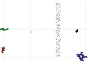
  $y$-direction, as shown by the slightly transparent spheres in figure 2(a). For cases L12–15 with larger particles, the area into which we initially place the particles is shaped like a square. We will demonstrate below that the influence of the initial particle configuration on the equilibrium number of flocs is negligible. Figure 2(a) shows a few typical floc configurations for case L7, with $Co = 0.5$, $\rho _s = 2.65$ and $\tilde D_p = 3.54 \times 10^{-2}$, at time $\tilde t = 95$, distinguished by colour. We recognize that some flocs have a compact structure (black, green and red), while others are more loosely aggregated (blue).

Figure 2. (a) Typical floc configurations observed at  $\tilde t = 95$ for case L7 with $Co = 0.5$, $\rho _s = 2.65$ and $\tilde D_p = 3.54 \times 10^{-2}$. Initially, the primary particles, shown as slightly transparent spheres, are randomly placed within a subsection of width $L_{ix} = 0.16$ and length $L_{iy} = 2$. (b) Temporal evolution of the average number of primary particles per floc $\bar N_p$ for the typical case L5 with $Co = 0.5$ and $\rho _s = 2.65$. Simulation data and a least-squares fit according to (3.1) are shown, with $N_{p,eq}$ and $t_{eq}$ denoting the equilibrium value of $\bar N_p$ and the beginning of the equilibrium stage, respectively. (c) Influence of the initial particle distribution on the flocculation for the typical case L7, with $Co = 0.5$ and $\rho _s = 2.65$. The initial particle distribution affects only the duration of the transient flocculation stage, but not the average floc size during the equilibrium stage. (d) Influence of the number of primary particles on the equilibrium floc size for the typical case L5, with $\rho _s = 2.65$, $Co = 0.5$ and $\phi \approx 3.8 \times 10^{-5}$. The equilibrium floc size is found to be largely independent of the number of primary particles. (e) Influence of the number of primary particles on the number of flocs for the typical case L5. ( f) Temporal evolution of the average number of primary particles per floc $\bar N_p$ for typical cases L15 and L5 with $\rho _s = 2.65$, $Co = 0.5$ and $\phi \approx 4 \times 10^{-5}$. Comparisons between one-way coupled simulations and equivalent, fully two-way coupled simulations show good agreement.
3.1. Flocculation and equilibrium stages
Consistent with our earlier work (Zhao et al. Reference Zhao, Vowinckel, Hsu, Köllner, Bai and Meiburg2020, Reference Zhao, Pomes, Vowinckel, Hsu, Bai and Meiburg2021), we consider different particles to belong to the same floc if their surface distance is less than half the range of the cohesive force. In terms of a physical force balance, breakage occurs when the net force pulling the particles apart is sufficiently strong to overcome the maximum of the cohesive force holding the particles together. Figure 2(b) shows the temporal evolution of the average number of primary particles per floc  $\bar N_p$ for the representative case L5, with $\rho _s = 2.65$ and $Co = 0.5$. We remark that an individual particle is considered to be the smallest possible floc. As the primary particles aggregate, $\bar N_p$ increases rapidly with time from its initial value of one, before levelling off around a constant value $N_{p,eq}$ that reflects a stable equilibrium between aggregation and breakage. Hence, we observe two distinct stages of the flow, viz. an initial flocculation stage and a subsequent equilibrium stage, consistent with previous experimental observations (Winterwerp et al. Reference Winterwerp, Manning, Martens, de Mulder and Vanlede2006; Son & Hsu Reference Son and Hsu2008; Tran et al. Reference Tran, Kuprenas and Strom2018).
In order to obtain a quantitative criterion for the ending of the flocculation stage and the beginning of the equilibrium stage, we employ a fitting model for  $\bar N_p$ of the form
 \begin{equation} {\bar N_p} = (1-N_{p,eq})B^{\tilde t} + N_{p,eq}. \end{equation}
A least-squares fit yields the coefficient  $B = 0.9766$ and the equilibrium average floc size $N_{p,eq} = 10.87$ for case L5, with a coefficient of determination value $R$-squared of 0.8. We define the first instant when $\bar N_p = N_{p,eq}$ as the beginning of the equilibrium stage $t_{eq}$, as shown in figure 2(b).
3.2. Influence of the initial particle configuration on the flocculation dynamics
We carefully assessed the influence of the initial particle distribution on the flocculation dynamics by varying the width  $L_{ix}$ in figure 2(a). We note that all particles are initially at rest and separate from each other. Figure 2(c) shows the evolution of the average number of primary particles per floc $\bar N_p$ for case L7, for various initial distributions. The density ratio and the cohesive number are fixed as $\rho _s = 2.65$ and $Co = 0.5$. We find that while a more dilute initial particle distribution slows down the flocculation process, it does not affect the average equilibrium floc size, which is the focus of the present investigation.
3.3. Influence of the primary particle number
To assess the influence of the number of primary particles on the equilibrium floc size, we compared simulations with  $N = 30\unicode{x2013}3000$ initial particles. Figure 2(d) presents the evolution of the average number of primary particles per floc $\bar N_p$ for different $N$. Figure 2(e) shows the evolution of the number of flocs $N_f$ for different $N$ accordingly. The primary particle size, the density ratio and the cohesive number are kept constant at $\tilde D_p = 2.74 \times 10^{-2}$, $\rho _s = 2.65$ and $Co = 0.5$. The domain size $\tilde L_x \times \tilde L_y$ varies with $N$, to keep the particle volume fraction fixed at $\phi \approx 3.8 \times 10^{-5}$. The initial local particle concentration was different in all three simulations, yielding different transient behaviours. The equilibrium floc size $N_{p,eq}$ reflecting the balance between breakage and aggregation depends only on the number of primary particles per unit domain when other governing parameters are fixed. We find that $N_{p,eq}$ is statistically independent of the number of primary particles $N$ once $N > N_{p,eq}$. The fluctuations of the average floc size during the equilibrium stage become smaller with for increasing particle numbers. This confirms that the value $N = 100$ employed in most of our simulations is sufficient for obtaining insight into the equilibrium stage of small flocs such as those considered here.
3.4. Comparison of flocculation dynamics in one-way and two-way coupled simulations
The one-way coupled simulation approach outlined above does not account for the effect of the particles on the fluid motion. Several previous investigations had considered the influence of two-way coupling, such as the shielding of the innermost particles in a large floc, which can have a major impact on the agglomerate breakup (Dizaji & Marshall Reference Dizaji and Marshall2017; Chen et al. Reference Chen, Li and Marshall2019). In order to demonstrate the ability of the one-way coupled approach to capture the aggregation of small flocs, we now provide a comparison between one-way and two-way coupled simulations. For the two-way coupling approach, we employ the immersed boundary method implemented in Vowinckel et al. (Reference Vowinckel, Withers, Luzzatto-Fegiz and Meiburg2019) to describe the particle–fluid interactions, and we use the spectral approach of Eswaran & Pope (Reference Eswaran and Pope1988) to generate statistically stationary turbulence. We remark that the present one-way coupled approach is sometimes referred to as ‘three-way coupled’, while the current two-way coupling is also regarded as ’particle-resolved four-way coupling’ by some previous researchers (Zhu et al. Reference Zhu, He, Zhao, Vowinckel and Meiburg2022). Additional information on the two-way coupled simulations is provided in Appendix B.
Figure 2( f) presents the temporal evolution of  $\bar N_p$ for typical cases L5 and L15, with $\rho _s = 2.65$ and $Co = 0.5$. When the flocculation is relatively weak (such as case L15 shown by dashed lines), the evolution of $\bar N_p$ is very similar for the one-way and two-way coupled simulations, since the modification of the local fluid flow by small flocs with few primary particles is limited. When the flocculation becomes stronger (such as case L5 shown by solid lines), two-way coupling results in a somewhat faster floc growth, although the average floc size during the equilibrium stage, $N_{p,eq}$, which is the focus of the present investigation, remains very similar. We conclude that one-way coupled simulations are able to provide insight into the aggregation of small flocs such as those considered here. Consequently, the one-way coupled Taylor–Green flow provides an efficient approach for analysing the formation of moderate-size flocs in turbulence. We expect that two-way coupled simulations will be required for analysing the dynamics of very large flocs (Yao & Capecelatro Reference Yao and Capecelatro2021).
3.5. Influence of the governing parameters
Recall that for a constant dimensional particle size and fluid properties,  $\tilde D_p \sim \sqrt {G}$, so that we can assess the influence of the dimensional shear rate $G$ by varying $\tilde D_p$. Towards this end, figure 3(a) demonstrates the influence of $\tilde D_p$, and hence $G$, on the average equilibrium floc size $N_{p,eq}$ for $Co=0.002$ and $Co = 0.5$, respectively. The other parameters are kept constant at $\rho _s = 2.65$ and $\phi \approx 4 \times 10^{-5}$. As $\tilde D_p$ (and hence the shear rate $G$) increases, $N_{p,eq}$ grows at first, then peaks and subsequently decays. Consequently, the simulations demonstrate that, for primary particles of the same size, intermediate shear rates produce the largest average floc size. This represents a central finding of the present investigation, and is consistent with previous experimental observations by He et al. (Reference He, Nan, Li and Li2012), Serra et al. (Reference Serra, Colomer and Logan2008) and Wang et al. (Reference Wang, Nan, Ji and Yang2018), who analysed the influence of the shear rate on the average floc size for different sediment types. For certain fluid/sediment combinations, these authors reported the existence of an optimal intermediate shear rate that gives rise to the largest average floc size. Figure 3(a) furthermore shows that, as $Co$ increases, the peak value of $N_{p,eq}$ grows and shifts to larger shear rates. Figure 3(b) presents $N_{p,eq}$ as function of the Stokes number $St$, for the same $Co$,
$Co$,  $\rho _s$ and $\phi$ as figure 3(a).

Figure 3. (a) Equilibrium value  $N_{p,eq}$ as function of the shear rate $G$, for different $Co$ values, with $\rho _s = 2.65$ and $\phi \approx 4 \times 10^{-5}$; (b) $N_{p,eq}$ as function of the Stokes number $St$, with the same $\rho _s$ and $\phi$ as (a). The relationship closely follows a log-normal distribution.
Figure 4(a) presents the average equilibrium floc size  $N_{p,eq}$ as a function of the shear rate, for different density ratios $\rho _s$, with $Co = 0.002$ and $\phi = 4\times 10^{-5}$. For larger $\rho _s$, the peak value of $N_{p,eq}$ grows and shifts to smaller $\tilde D_p$ (and hence smaller shear rates). Figure 4(b–d) shows a non-monotonic relationship between $N_{p,eq}$ and $St$, for $\rho _s = 5, 8, 10$, respectively. By comparing cases L8, L9 and L10 for fixed values of $\rho _s$ and $Co$ (not shown), we find that the pseudo-volume fraction $\phi$ only weakly affects $N_{p,eq}$. This finding agrees with experimental observations by Serra et al. (Reference Serra, Colomer and Logan2008), who performed experiments at different particle volume fractions ( $2.0 \times 10^{-5} < \phi < 1.0 \times 10^{-4}$), without noticing appreciable differences in $N_{p,eq}$ for the same shear rate.

Figure 4. (a) Equilibrium value  $N_{p,eq}$ as a function of the dimensionless particle size $\tilde D_p$ (proportional to $G^{0.5}$), for different density ratios $\rho _s$. (b–d) Show the relation between $N_{p,eq}$ and the Stokes number $St$ for $\rho _s = 5, 8, 10$, respectively. The cohesive number $Co = 0.002$ and the pseudo-volume fraction $\phi \approx 4 \times 10^{-5}$ are fixed.
In order to obtain insight into the mechanisms responsible for the non-monotonic relationship between  $\tilde D_p$ and $N_{p,eq}$, we keep track of the evolution of three different types of flocs over a suitably specified time interval ${\rm \Delta} \tilde t = 2$: (a) those flocs that maintain their identity, i.e. they consist of the same primary particles at the start and the end of the time interval; (b) those that add additional primary particles while keeping all of their original ones; and (c) all others, i.e. all those that have undergone a breakage event during the time interval. We define the fractions of these respective groups as $\theta _{id}$, $\theta _{ad}$ and $\theta _{br}$, with $\theta _{id}$ + $\theta _{ad} + \theta _{br} = 1$. Figure 5 shows the evolution of $\theta _{br}$ and $\theta _{ad}$ for the three cases L1 ( $\tilde D_p = 1.22 \times 10^{-2}$), L5 ( $\tilde D_p = 2.74 \times 10^{-2}$) and L11 ( $\tilde D_p = 8.66 \times 10^{-2}$), respectively, with fixed values $Co = 0.002$, $\rho _s = 2.65$ and $\phi \approx 4 \times 10^{-5}$. It clearly demonstrates that floc collisions and break-up processes remain active throughout the entire simulations. The red symbols in figure 3(a) show that of these three cases L5 has the largest average equilibrium floc size. Figure 5(a) shows that $\theta _{br}$ generally increases with $\tilde D_p$, while, figure 5(b) demonstrates that for the early flocculation stage ( $\tilde t < 10$) the intermediate case L5 has the largest fraction of growing flocs. At this intermediate value of $\tilde D_p$, the primary particles rapidly aggregate, but the turbulent stresses are not large enough to easily break the flocs.

Figure 5. Temporal evolution of the fraction of flocs that over the time interval  ${\rm \Delta} \tilde t = 2$, with $Co = 0.002$, $\rho _s = 2.65$, $\phi \approx 4 \times 10^{-5}$, (a) undergo breakage; (b) add primary particles.
3.6. Limitation of the aggregate size by the vortex size
In order to capture the physical floc size in the two-dimensional cellular Taylor–Green vortex flow, we define a characteristic scale  $L_f$ of the floc as
 \begin{equation} L_f = 2 \max(\| \boldsymbol x_{p,i} - \boldsymbol x_c \|) + D_p,\quad 1 \leqslant i \leqslant N, \end{equation}
where  $\boldsymbol x_{p,i}$ denotes the position of the centre of primary particle $i$, and $\boldsymbol x_c = \sum _{i=1}^{N} \boldsymbol x_{p,i} / N$ is the floc's centre of mass. We remark that $L_f$ is known as the Feret diameter of flocs in turbulent flow.
We track the average value  $\bar L_f$ and the maximum value $\max (L_f)$ of floc size with time. Figure 6(a) displays the temporal evolution of size ratio between flocs and the individual vortex, with $Co = 0.5$, $\rho _s = 2.65$, $\tilde D_p = 5.00 \times 10^{-2}$ and $\phi = 3.64 \times 10^{-5}$. The average floc size remains smaller than the Kolmogorov length scale ( $\bar L_f / \eta < 1$), while the size of the biggest floc can temporarily exceed $\eta$ before rapidly decreasing. This finding is consistent with previous experimental observations by Stricot et al. (Reference Stricot, Filali, Lesage, Spérandio and Cabassud2010) and Braithwaite et al. (Reference Braithwaite, Bowers, Nimmo Smith and Graham2012), who found that big flocs cannot resist the turbulent stresses for long, and that they are torn apart quickly. For sufficiently strong turbulence the median floc size should be of the same order as the smallest turbulent eddies.

Figure 6. (a) Temporal evolution of the ratio between the physical floc size  $L_f$ and the Kolmogorov length scale $\eta$, for $Co = 0.5$, $\rho _s = 2.65$, $\tilde D_p = 5.00 \times 10^{-2}$, $\phi = 3.64 \times 10^{-5}$. Here, $\bar L_f$ and $\max (L_f)$ denote the average floc size and the maximum floc size at time $\tilde t$, respectively. (b) Ratio between the equilibrium floc size $L_{f,eq}$ and the Kolmogorov length scale $\eta$, as well as between $L_{f,eq}$ and the dimensional diameter of primary particles $D_p$, for different Stokes numbers $St$, with $Co = 0.5$, $\rho _s = 2.65$, $\phi \approx 4 \times 10^{-5}$.
Figure 6(b) shows the ratio between the equilibrium floc size  $L_{f,eq}$ and the Kolmogorov length scale $\eta$ for different Stokes numbers $St$, with $Co = 0.5$, $\rho _s = 2.65$ and $\phi \approx 4 \times 10^{-5}$. Within the present range of parameters shown in table 1, the equilibrium floc size remains smaller than the physical size of an individual vortex. The relation between the length ratio $L_{f,eq} / D_p$ and the Stokes number $St$ is shown as well. As the dimensional size of the primary particles $D_p$ is fixed, we find that intermediate $St$ (and hence intermediate shear rate) produces the maximum physical floc size $L_{f,eq}$, similar to figure 3(b) in which the floc size is given in terms of the number of particles.
3.7. Floc size distribution during the equilibrium stage
Figure 7 displays the equilibrium floc size distribution for different values of  $\tilde D_p$, i.e. different shear rates. The other parameters are approximately constant. Here, $N_p$ denotes the number of primary particles in a floc, while $L_{f,eq} / D_p$ represents the physical size ratio between the floc and the primary particle and $N_f$ indicates the number of flocs. Figure 7(a,b) indicates that the distribution peaks at small size values for the largest and the smallest $\tilde D_p$, while it shifts to larger values of floc size for intermediate values of $\tilde D_p$. This is consistent with our earlier observation that the average equilibrium floc size has a maximum for intermediate values of $\tilde D_p$, cf. figures 3(a) and 6(d).

Figure 7. Equilibrium floc size distribution for different  $\tilde D_p$. Here, $\rho _s = 2.65$, $\phi \approx 4 \times 10^{-5}$, $Co = 0.002$. (a) Floc size is in terms of the number of primary particles per floc $N_p$. (b) Floc size is denoted by the size ratio $L_{f,eq} / D_p$.
3.8. A model for the average floc size during the equilibrium stage
According to Khelifa & Hill (Reference Khelifa and Hill2006), for flocs with fractal dimension  $n_f$, the mean equilibrium floc size is related to the average number of primary particles per floc as
 \begin{equation} \tilde D_{f,eq} = \tilde D_p N_{p,eq}^{1/n_f}. \end{equation}
 Figure 3(a) suggests that the relation between  $\tilde D_p$ and $N_{p,eq}$ can be fitted by a log-normal probability density function of the form
 \begin{equation} N_{p,eq} = a d_2 + \frac{b d_2}{\sigma \sqrt{2 {\rm \pi}} \tilde D_p d_1} \exp\frac{-[\ln (\tilde D_p d_1) - c]^2}{2 \sigma^2}, \end{equation}
where  $a$,
$a$,  $b$,
$b$,  $d_1$ and $d_2$ represent empirical coefficients, while $c$ denotes the mean and $\sigma$ the standard deviation of the natural logarithm of $\tilde D_p$, respectively. The simulation results over the parameter ranges given in table 2 are processed via a least-squares fit, we obtain
 \begin{gather} a^{{-}1} = 0.0924 + 0.0129(\ln{Co})^2 + 3.628\exp{(-\rho_s)}, \end{gather}
 \begin{gather}b^{{-}1} = 1.455 - 0.9718 \ln{Co} - 23.66\exp{(-\rho_s)}, \end{gather}
 \begin{gather}c^{{-}1} ={-}0.2727 + 0.2080 Co \ln{Co}, \end{gather}
 \begin{gather}\sigma^{{-}1} = 4.729 + 1.504 \rho_s^2 \ln\rho_s - 1.109 \rho_s^{2.5}. \end{gather}
For the present cellular model flow the values  $d_1 = d_2 = 1$ in (3.4) yield optimal agreement with the simulation data, with a fitting deviation of ${\pm }30\,\%$. For real turbulent flows, we can determine $d_1$ and $d_2$ by calibrating with available experimental data by other investigators, as follows. In order to capture representative sediment transport applications, we employ the data from four sets of experiments described in the literature, cf. figure 8, which yields the values of $d_1$ and $d_2$. We note that our simulations explore the influence of all of the experimental parameters except the pH value, whose influence will be investigated in a future study. As seen in figure 8, $d_2 = 5$ captures all of the experiments, while $d_1$ varies within the range from 0.5 to 3.5. In summary, the simulation results indicate that the present model (3.3)–(3.8) can successfully predict the average equilibrium floc size for a wide range of sediment transport applications characterized by the dimensionless input parameters $\tilde D_p$, $\rho _s$, $Co$ and $d_1$. These capture the influence of the particle size, shear strength, density ratio and cohesive force, respectively. Once the model has been calibrated for one particular fluid/particle combination and a given flow field, it is expected to be used to predict the floc size distributions for the same fluid/particle combination at different volume fractions, particle sizes and turbulence properties.

Figure 8. Calibration of the empirical coefficients  $d_1$ and $d_2$ in the present model with experimental data. (a) Experiments of Serra et al. (Reference Serra, Colomer and Logan2008) for latex particles in salt water ( $n_f = 2$, $A_H = 1.3 \times 10^{-20}\,{\rm J}$), yield $d_1 = 3$. (b) Experiments of He et al. (Reference He, Nan, Li and Li2012) for a Kaolin clay suspension ( $n_f = 1.12$, $A_H = 5.0 \times 10^{-20}\,{\rm J}$), yield $d_1 = 3.5$. (c) Experiments of Mietta et al. (Reference Mietta, Chassagne, Manning and Winterwerp2009) for natural mud in an estuary ( $n_f = 2$, $A_H = 1.0 \times 10^{-20}\,{\rm J}$), yield $d_1 = 0.5$. (d) Experiments by Wang et al. (Reference Wang, Nan, Ji and Yang2018) for a Kaolin clay solution with humic acid ( $n_f = 1.12$, $A_H = 5.0 \times 10^{-20}\,{\rm J}$), yield $d_1 = 1.7$. Noted that all of the experiments yield the constant $d_2 = 5$. For details of the experiments, we refer the reader to the cited works.
4. Conclusions
We have presented one-way coupled simulations to study the influence of the shear rate on the flocculation of suspended cohesive particles in a model turbulent flow field. For select parameter combinations, the one-way coupled results were confirmed by two-way coupled simulations. The computational model captures Stokes drag, cohesion, lubrication and direct contact forces. After a transient flocculation stage, we observe a statistically steady equilibrium stage where aggregation and breakage balance each other. The simulations reproduce the non-monotonic relationship between the equilibrium floc size and the turbulent shear rate observed by earlier experiments. They suggest that an intermediate shear rate results in the largest flocs, as it promotes preferential concentration of the primary particles without producing sufficiently large stresses to break up the emerging aggregates. We find that this optimal intermediate shear grows for stronger cohesion and smaller density ratios, while it does not exhibit a strong influence of the particle volume fraction. The relationship between the equilibrium floc size and the shear rate displays a log-normal shape, which enables us to propose a model for predicting the equilibrium floc size for different shear rates. Upon calibration with several experimental data sets, the proposed model yields good agreements with measured data across a wide range of fluid and sediment properties.
Funding
K.Z. is supported by NSFC grants 51888103, 52206208, 52276161 and xpt022022016, as well as by the China Postdoctoral Science Foundation BX2021234 and 2022M712524. E.M. acknowledges support through NSF grants CBET-1803380 and OCE-1924655, as well as through Army Research Office grant W911NF-18-1-0379. B.V. gratefully acknowledges support through German Research Foundation (DFG) grant VO2413/2-1. T.J.H. received support through NSF grant OCE-1924532. Computational resources are supported by XSEDE grant TG-CTS150053.
Declaration of interests
The authors report no conflict of interest.
Appendix A. Elastic deformation of cohesive spheres
Two distinct frameworks have been developed for modelling cohesive forces: (i) the Derjaguin–Muller–Toporov (DMT) framework, in which forces are additive because particles do not overlap substantially (Derjaguin, Muller & Toporov Reference Derjaguin, Muller and Toporov1975); and (ii) the Johnson–Kendall–Roberts (JKR) framework, where the cohesive forces scale with the contact area and particles deform upon contact (Johnson, Kendall & Roberts Reference Johnson, Kendall and Roberts1971). The Tabor parameter  $\mu _T$ helps to decide between those two frameworks, as it reflects the ratio of the elastic deformation and the cohesive interaction range (Tabor Reference Tabor1977)
 \begin{equation} {\mu_T} = {\left(\frac{R_{ij} {({\rm \Delta} \gamma)}^2}{{E^*}^2 {z_0}^3} \right)}^{1/3}. \end{equation}
Here, the reduced particle radius  $R_{ij} = D_p /4$, the work of adhesion ${\rm \Delta} \gamma = 2\gamma$, the combined elastic modulus of the spheres $E^* = E / {2(1 - {\nu _T}^2)}$, the effective elastic modulus $E$ and the Poisson number $\nu _T$. Chen et al. (Reference Chen, Li and Marshall2019) described the equilibrium separation as $z_0 = (9 {\rm \pi}\gamma {R_{ij}}^2/E)^{1/3}$. Yao & Capecelatro (Reference Yao and Capecelatro2021) expressed the surface energy of the particle as $\gamma = A_H / 24 {\rm \pi}\delta ^2$. Marshall & Li (Reference Marshall and Li2014) defined the length $\delta = 0.165\,{\rm nm}$.
As shown in table 1, the particle diameter in the present simulations  $D_p = 5 \,\mathrm {\mu }{\rm m}$ is fixed, and the range of the Hamaker constant is $2.0 \times 10^{-21}\,{\rm J} \leq A_H \leq 5.0 \times 10^{-19}\,{\rm J}$, yielding the range of the surface energy $9.8 \times 10^{-4}\,{\rm J}\,{\rm m}^{-2} \leq \gamma \leq 2.4 \times 10^{-1}\,{\rm J}\,{\rm m}^{-2}$. For typical natural particles, the Tabor parameter values are smaller than 0.03, as listed in table 3. Actually, due to the present values of $R_{ij}$ and ${\rm \Delta} \gamma$ are very small, the Tabor parameter in the simulations is typically smaller than 0.1, even though the values of the elastic modulus and the Poisson number varied in the wide ranges, i.e. $E > 0.01\,{\rm GPa}$ and $0 < \nu _T < 1$. The Johnson–Greenwood mapping introduced by Johnson & Greenwood (Reference Johnson and Greenwood1997) indicates that the magnitude of the pull-off force varied continuously from the DMT value for $\mu _T < 0.1$ to the JKR value for $\mu _T > 5$. Hence, the additive DMT model is more appropriate to describe the cohesion and collision between particles for these cases with small Tabor numbers.
Table 3. Tabor parameter  $\mu _T$ of typical natural sediments, for the present particle diameter $D_p = 5\,\mathrm {\mu }{\rm m}$, and surface energies ranging from $\gamma = 0.00098\unicode{x2013}0.24\,{\rm J}\,{\rm m}^{-2}$. Values of the elastic modulus $E$ and the Poisson number $\nu _T$ are cited from Hamilton (Reference Hamilton1971).

Appendix B. Two-way coupled simulations
In order to validate the one-way coupled simulations, we conduct grain-resolved two-way coupled simulations for two typical cases. The immersed boundary method is employed to describe the particle–fluid interactions as implemented in Vowinckel et al. (Reference Vowinckel, Withers, Luzzatto-Fegiz and Meiburg2019). Sometimes this two-way coupled approach is referred to as ’particle-resolved four-way coupled’. We consider the grain-resolved two-way coupled motion of suspended cohesive particles in three-dimensional, incompressible homogeneous isotropic turbulence. The motion of the single-phase fluid with constant density  $\rho _f$ and kinematic viscosity $\nu$ is governed by
 \begin{gather} \boldsymbol{\nabla} \boldsymbol{\cdot} \boldsymbol{u_f} = 0, \end{gather}
 \begin{gather}\frac{\partial \boldsymbol{u_f} }{\partial t} + (\boldsymbol{u_f} \boldsymbol{\cdot}\boldsymbol{\nabla}) \boldsymbol{u_f} ={-} \frac{1}{\rho_f} \boldsymbol{\nabla} p + \nu \nabla^2 \boldsymbol{u_f} + \boldsymbol F_{tur} + \boldsymbol F_{ibm}, \end{gather}
where  $\boldsymbol {u_f} = (u_f, v_f, w_f)^{\rm T}$ denotes the fluid velocity vector and $p$ indicates the hydrodynamic pressure. We employ the spectral approach of Eswaran & Pope (Reference Eswaran and Pope1988) to obtain the forcing term $\boldsymbol F_{tur}$, which generates and maintains statistically stationary turbulence, as implemented in Chouippe & Uhlmann (Reference Chouippe and Uhlmann2015). Here, $\boldsymbol F_{tur}$ is non-zero only in the low-wavenumber band where the wavenumber vector $|\boldsymbol \kappa | < \kappa _f$, with $\kappa _f = 2.3\kappa _0$ and $\kappa _0 = 2 {\rm \pi}/ L_0$, with $L_0$ denoting the length of the physical domain. The origin $\boldsymbol \kappa = 0$ is not forced. In addition to the cutoff wavenumber $\kappa _f$, the random forcing process is governed by the dimensionless parameter $D_s = \psi ^2 T_0 L_0^4 / \nu ^3$, where $\psi ^2$ and $T_0$ indicate the variance and the time scale of the random process, respectively. Regarding the details of evaluating $\boldsymbol F_{tur}$ from $\kappa _f$ and $D_s$, we refer the reader to the original work by Eswaran & Pope (Reference Eswaran and Pope1988); $\boldsymbol F_{ibm}$ represents an artificial volume force introduced by the immersed boundary method (Vowinckel et al. Reference Vowinckel, Withers, Luzzatto-Fegiz and Meiburg2019).
We calculate the motion of each individual spherical particle by solving an ordinary differential equation for its translational velocity and angular velocity,
 \begin{gather} m_p \frac{\mathrm{d} {\boldsymbol u}_{p,i}}{\mathrm{d} t} = \oint_{\varGamma_p} {{\boldsymbol \tau} \boldsymbol{\cdot} {\boldsymbol n}\,\mathrm{d} A} + \sum_{j=1,j \ne i}^{N}({\boldsymbol F}_{con,ij} +{\boldsymbol F}_{lub,ij} + {\boldsymbol F}_{coh,ij}), \end{gather}
 \begin{gather}I_p \frac{\mathrm{d}{\boldsymbol \omega}_{p,i}}{\mathrm{d} t} = \oint_{\varGamma_p} {{\boldsymbol r} \times ({\boldsymbol \tau} \boldsymbol{\cdot} {\boldsymbol n})\,\mathrm{d} A} + \sum_{j=1,j \ne i}^{N}({\boldsymbol T}_{con,ij} + {\boldsymbol T}_{lub,ij}), \end{gather}
where  $\boldsymbol \tau$ denotes the hydrodynamic stress tensor, $\boldsymbol r$ is the position vector of the surface point with respect to the centre of mass of a particle.
In two-way coupling simulations, we set the number of primary particles  $N = 82$ and the size ratio between the domain and the primary particles $L_0/D_p = 102.4$, yielding the volume fraction of particles $\phi \approx 4.0 \times 10^{-5}$. The density ratio $\rho _p/\rho _f = 2.65$ and the cohesive number $Co = 0.5$ are fixed. The triply periodic computational domain is a cube with the number of grid cells $N_x \times N_y \times N_z = 1024 \times 1024 \times 1024$. The length ratios between the Kolmogorov scale and the size of primary particles are $\eta /D_p = 36$ and $\eta /D_p = 3.3$ for cases L5 and L15, respectively.


 Open access