


1. Introduction
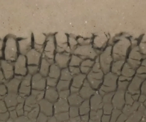
The freezing of colloidal and nano suspensions is of increasing importance in composite materials science, Earth and planetary science, cryobiology, microfluidics, food engineering and chromatography (Rempel Reference Rempel2010; Qian & Zhang Reference Qian and Zhang2011; Deville Reference Deville2013; Henderson et al. Reference Henderson, Ladewiq, Haylock, MacLean and O'Connor2013; Pawelec et al. Reference Pawelec, Husmann, Best and Cameron2014). Owing to the complexity of such systems, which involve flow and phase change in multicomponent suspensions and porous media, the development of models to predict ice morphology is challenging. During solidification of multi-component melts, solutions or alloys, the solid phase often forms an intricate microstructure of dendritic crystals aligned with the thermal gradient (figure 1a) within what is called a mushy layer. In these contexts, ‘microstructure’ refers to formations on a scale that is small compared with the dimensions of the partially solidified region or casting. Similarly intricate microstructures can form during the freezing of colloidal suspensions (figure 1b–d) but with a greater variety of patterns, including dendrites aligned with the thermal gradient (figure 1b), lenses perpendicular to the thermal gradient (figure 1c) and polygonal structures (figure 1d). Some of these structures, particularly the dendritic ones, arise from morphological instability of the interface between frozen solvent (ice) and unfrozen solution or colloidal suspension (Peppin, Worster & Wettlaufer Reference Peppin, Worster and Wettlaufer2007; El Hasadi & Kodadadi Reference El Hasadi and Kodadadi2015) but others form by regelative processes within partially frozen colloid (O'Neill & Miller Reference O'Neill and Miller1985; Rempel, Wettlaufer & Worster Reference Rempel, Wettlaufer and Worster2004; Anderson & Worster Reference Anderson and Worster2012).

Figure 1. Mushy layers formed in different materials frozen in vertical temperature gradients. (a) Dendritic mushy layer of ammonium chloride crystals formed from aqueous solution (photo M.A. Hallworth). (b) Dendritic mushy layer of ice platelets formed from a dilute suspension of bentonite clay in water (photo S. Peppin). (c) Mushy layer of horizontal lenses (lower layer) formed from a suspension of alumina particles in water (Anderson & Worster Reference Anderson and Worster2012). (d) Polygonal mushy layer formed from a concentrated suspension of bentonite clay in water (photo S. Peppin). The photographs in (a,b,d) are a few mm across, while that in (c) is approximately 3 cm across.
Mathematical models of mushy layers formed from solutions (Worster Reference Worster1992) often describe them with continuum equations, averaged over the microstructure, which can be used to predict the spatial distribution and temporal evolution of the solid fraction as well as any macro-segregation caused by solute diffusion or convection of the interstitial liquid. Here, we describe an approach to modelling mixed-phase regions (mushy regions) within solidifying colloidal suspensions that is independent of their microstructural morphology and independent, therefore, of their origin. We consider only hard-sphere interactions between the colloidal particles, though cohesion between particles can be an important influence on microstructural evolution.
2. Phase diagram
Key to the description of phase change in mixtures is the phase diagram, which shows which phases exist in thermodynamic equilibrium at a given temperature, composition and pressure. Here, we consider cases in which the external bulk pressure is constant and so concern ourselves with phase diagrams with respect to temperature and composition only. We also restrict attention to systems that do not contain solid solutions, so that any solid that forms contains only the pure solvent material. For convenience and definiteness, we refer to the solvent or suspending fluid as ‘water’ and its solid phase as ‘ice’. We define the bulk, thermodynamic pressure  $P$ as the pressure averaged over a thermodynamically representative region of the mixture, and the pervadic pressure $p$ as the pressure measured in solvent that is in equilibrium with but separated from the mixture by a semi-permeable membrane (figure 2a, Peppin, Elliot & Worster Reference Peppin, Elliot and Worster2005). The pervadic pressure is related to the specific chemical potential of the solvent $\mu _c$ by $\textrm {d}\mu _c = (1/\rho )\,\textrm {d}p - s\,\textrm {d}T$, where $s$ is the specific entropy of the solvent and $\rho$ is its density, which provides a helpful link in the context of solutions. However, in a concentrated suspension forming a porous medium, the pervadic pressure is best thought of as the pore pressure driving flow of the interstitial solvent. The generalised osmotic pressure $\varPi$ is defined by
 \begin{equation} \varPi = P - p. \end{equation}
Figure 2. (a) A defining sketch illustrating the macroscopic measurement of bulk pressure  $P$ and pervadic pressure $p$ in the case of a dilute suspension or solution (upper part) and in the case of a concentrated suspension (lower part). In each case, the bulk pressure is that measured by a transducer (narrower red boundary) that samples a thermodynamically representative region containing both solute (particles) and solvent (suspending fluid), while the pervadic pressure is measured by a transducer immersed in pure solvent separated by a semi-permeable membrane (dashed line) from the colloidal suspension but in equilibrium with it. (b) The equilibrium configuration between a colloidal suspension and solidified solvent (ice). The phase boundary acts as a semi-permeable membrane, allowing exchange of solvent but not particles.
Figure 2(b) shows a colloidal suspension in equilibrium with frozen solvent, from which we see that the solid–liquid interface acts as a semi-permeable membrane in the case that solid solutions cannot occur. The generalised Clausius–Clapeyron equation, considering the solvent alone, gives that
 \begin{equation} \rho L\frac{T_m - T}{T_m} = p_s - p_l, \end{equation}
where  $T$ is absolute temperature, $T_m$ is the absolute freezing temperature of the pure solvent, $\rho$ is the density of its solid phase but is assumed here to be independent of phase for simplicity, $L$ is the specific latent heat of fusion and $p_s$ and $p_l$ are the pressures in the solid and liquid phases of the solvent on either side of the phase boundary. With reference to figure 2(b), we see that $p_s = P$ and $p_l = p$ and so we can determine the equilibrium (Liquidus) temperature $T_L$ of a mixture of concentration (particle volume fraction) $\phi$ to be
 \begin{equation} T_L = T_m - \frac{T_m}{\rho L}\varPi(\phi). \end{equation}
 The osmotic pressure  $\varPi (\phi )$ of a hard-sphere suspension when the absolute temperature $T\approx T_m$ is given by $\varPi = k_B T_m \phi /v(R)$ when $\phi \ll 1$, where $k_B$ is Boltzmann's constant, $R$ is the radius of the hard spheres (assumed mono-disperse) and $v(R) = 4({\rm \pi} R^3)/3$ is the volume of each sphere (Einstein Reference Einstein1956). It varies inversely with $\phi _c - \phi$ as $\phi$ approaches the close-packed limit $\phi _c$ (Woodcock Reference Woodcock1981). For simplicity and clarity of presentation, we consider here an approximate functional form of the osmotic pressure that is the leading-order Padé approximant between these limits
 \begin{equation} \varPi(\phi, R) = \frac{k_B T_m }{v(R)}\frac{\phi}{(1 - \phi/\phi_c)}. \end{equation}
The key qualitative results of this paper result from the divergence as  $\phi \to \phi _c$, which is a necessary feature of the constitutive relationship for the osmotic pressure. Quantitatively, there is not much room for manoeuvre in this expression once the limiting behaviours are accounted for. In short, the results of this paper do not depend significantly on the precise form of (2.4).
Equation (2.4) can be used in (2.3) to determine the liquidus temperature  $T_L(\phi , R)$ as a function of particle fraction and size. This is illustrated in figure 3. We see that when $R = 0.2\ \textrm {nm}$, which is roughly comparable to the ionic radii of small molecular solutes (e.g. chlorine ions (0.18 nm) and sodium ions (0.1 nm)), the liquidus curve is characteristic of an aqueous salt solution. However, as the particle size increases, the liquidus temperature approaches the constant value $T_m$ except for concentrations very close to the close-packed limit $\phi _c - \phi \ll 1$. This behaviour can be understood by noting that the prefactor in (2.4) is very large when $R$ is small and so the liquidus temperature changes a lot for only small changes in $\phi$. Therefore, for modest undercooling, the particle volume fraction is small and the liquidus curve is approximately linear. Conversely, when $R$ is large, changes in $\phi$ cause a negligible reduction in the freezing temperature, which remains close to $T_m$, until $\phi$ approaches $\phi _c$.

Figure 3. Representative phase diagrams for hard-sphere, colloidal suspensions containing mono disperse particles for different particle radii  $R$ showing the freezing (liquidus) temperature as a function of particle concentration $\phi$. As $R$ increases, the liquidus temperature tends towards the constant bulk freezing temperature of the solvent $T_m$ except very close to the close-packed limit $\phi =\phi _c$. Note the reduced range of the abscissa and increased range of the ordinate in (a) compared with (b,c). The ice-entry temperatures $T_E$ are approximately $-1000\,^{\circ }\textrm {C}$, $-300\,^{\circ }\textrm {C}$ and $-60\,^{\circ }\textrm {C}$ for the three cases shown, and so do not enter the diagrams.
In this paper, we consider very small particles and modest undercoolings and so ignore the possibility of the pore water freezing, which can happen when the temperature falls below the ice-entry temperature  $T_E = T_m - (T_m/\rho L)(2\gamma /R_f)$, where $\gamma$ is the surface energy of an ice–water interface and $R_f < R$ is a typical pore radius. For reference, for the water–ice system, $T_E \approx -1\,^{\circ }\textrm {C}$ when the particle size $R\approx 0.3\ \mathrm {\mu }\textrm {m}$. We will see later that the interesting cross-over in behaviour that we highlight in this paper happens for suspensions of nano particles with $R < 0.03\ \mathrm {\mu }\textrm {m}$, for which the ice-entry temperature is below $-10\,^{\circ }\textrm {C}$.
The advantage of our approximate liquidus relationship for analytical modelling is that it is readily inverted to give the colloidal concentration at the phase boundary
 \begin{equation} \phi = \phi_L(T, R) \equiv \left[\frac{K\phi_c}{T_m - T} + 1\right]^{-1}\phi_c \end{equation}
in terms of the temperature there, where  $K(R) = (T_m/\rho L)(k_B T_m/v(R))$ is the magnitude of the liquidus slope at $\phi = 0$.
3. Relative motion in colloidal suspensions
In a dilute solution or suspension, it is familiar to think of diffusion in terms of random walks of the molecules or particles, in the latter case associated with Brownian motion. The random walks taken by individual molecules give rise to the self-diffusion of a species and an intermingling of the molecules. This is illustrated in figure 4(a), in which the identical particles are tagged with either red or blue colours, which by self-diffusion become mixed statistically homogeneously in time. The self-diffusion decreases with particle size, as illustrated by the expression for Stokes–Einstein diffusion of dilute suspensions
 \begin{equation} D = \frac{k_B T}{6{\rm \pi}\mu R}, \end{equation}
where  $\mu$ is the dynamic viscosity of the suspending fluid. By this description, the particle flux relative to the suspending fluid is given by
 \begin{equation} -\phi \boldsymbol{q} = - D\boldsymbol{\nabla}\phi, \end{equation}
where  $\boldsymbol {q}$ is the fluid flux relative to the particles per unit area of mixture (the Darcy flux).

Figure 4. (a,c) A dilute suspension with concentration decreasing from left to right tends to a uniform concentration by self-diffusion of the particles in time (top to bottom). (b,d) A concentrated suspension with concentration decreasing from left to right tends to a uniform concentration by jostling limited by interstitial fluid flow from right to left (shown by arrow). Concentration gradients relax but the intermingling of particles is limited.
By contrast, in a concentrated suspension, illustrated in figure 4(b), although the self-diffusion is small, even negligible, inhomogeneities of concentration still relax by Brownian jostling of the particles, limited by the viscous drag of the suspending fluid through the interstices of the particle cluster. By Darcy's law
 \begin{equation} \boldsymbol{q} = -\frac{k}{\mu}\boldsymbol{\nabla} p, \end{equation}
where  $k(\phi )$ is the permeability of the particle cluster. If the bulk pressure $P$ is uniform then $\boldsymbol {\nabla } p = -\boldsymbol {\nabla }\varPi$ and so, comparing (3.2) and (3.3), we see that
 \begin{equation} D(\phi) = \frac{\phi k(\phi)}{\mu}\frac{\partial\varPi}{\partial\phi}. \end{equation}
In this paper, we use the same expression for the permeability
 \begin{equation} k(\phi) = \tfrac{2}{9}R^2 {(1 - \phi)^6/\phi} \end{equation}
that was used by Peppin, Elliot & Worster (Reference Peppin, Elliot and Worster2006), obtained empirically by Russel, Saville & Schowalter (Reference Russel, Saville and Schowalter1989). Note that the combination of (3.4) and (3.5) together with (2.4) reproduces (3.1) in the limit  $\phi \ll 1$.
This brief description is a summary of the derivation provided by Peppin et al. (Reference Peppin, Elliot and Worster2005). We see that the osmotic pressure  $\varPi (\phi )$ is central to an understanding of both flow and phase in these freezing colloidal systems. There are many hydrodynamic and thermodynamic studies to determine higher-order expansions of (3.1) for small but finite $\phi$, for example the seminal paper of Batchelor (Reference Batchelor1976) and later papers by Batchelor (Reference Batchelor1983), Brady (Reference Brady1993) and Marath & Wettlaufer (Reference Marath and Wettlaufer2019). However, for illustration and clarity of exposition, we use the simple expression (2.4) throughout this paper to describe both the phase diagram and the hydrodynamic interactions.
4. Solidification from a plane boundary
4.1. Fickian formulation
Similarity solutions for one-dimensional solidification of a colloidal suspension from a planar boundary were presented by Peppin et al. (Reference Peppin, Elliot and Worster2006). We present a simpler version of those solutions here as a precursor to our study of the mushy layers that can form at sufficiently large undercoolings. The problem solved is shown schematically in figure 5. We ignore latent heat release at the phase boundary and assume that the density and specific heat capacity are the same for particles and solute and independent of phase. Therefore, the temperature is given by
 \begin{equation} T(z, t) = T_{\infty} + (T_B - T_{\infty})\text{erfc}\,\eta, \quad \eta = \frac{z}{2\sqrt{\kappa t}}, \end{equation}
where  $T_B$ is the temperature of the boundary $z=0$, $T_{\infty }$ is the temperature far from the boundary and $\kappa$ is the thermal diffusivity.

Figure 5. A schematic diagram of the solidification of a colloidal suspension to produce a layer of pure frozen solvent (ice) separated from the unfrozen suspension by a planar interface. The particles rejected by the ice accumulate ahead of the ice in a concentration boundary layer. If the concentration of particles in the boundary layer approaches the close-packed limit then the boundary layer forms a porous medium of almost uniform particle concentration with a much thinner, diffuse boundary layer of rapid variation of particle concentration separating it from the original suspension.
If  $T_B < T_L(\phi _{\infty }, R)$, where $\phi _{\infty }$ is the uniform particle concentration far from the boundary, then ice will form against the boundary and push particles ahead of it. For given $R$, we write $D(\phi , R) = D(\phi )$ for brevity, and the concentration of colloidal particles ahead of the layer of ice satisfies a diffusion equation
 \begin{equation} \frac{\partial\phi}{\partial t} = \frac{\partial}{\partial z} \left[D(\phi)\frac{\partial\phi}{\partial z}\right], \end{equation}
with boundary conditions
 \begin{equation} \phi(h) = \phi_L(T(h)) \quad\text{and} \quad \phi \to \phi_{\infty} \quad\text{as}\ z \to \infty, \end{equation}
where  $h = 2\lambda \sqrt {\kappa t}$ is the thickness of the layer of ice determined by the interfacial condition expressing local conservation of solute
 \begin{equation} \phi \dot{h} = \left.-D(\phi)\frac{\partial \phi}{\partial z}\right\vert_{z = h+}. \end{equation}
 Equation (4.2) can be written as a pair of first-order equations in the similarity variable  $\eta$ as
 \begin{equation} \phi' = -2\frac{\kappa}{D(\phi)}q, \quad q' = -2\frac{\kappa}{D(\phi)}\eta q, \end{equation}
with boundary conditions
 \begin{gather} \phi = \phi_L \quad\text{and}\quad q = \lambda \phi_L \quad\text{at}\ \eta=\lambda, \end{gather}
 \begin{gather} \phi\to\phi_{\infty} \quad\text{as}\ \eta\to\infty, \end{gather}
where  $\phi _L = \phi _L(T)$ is given by (2.5). Note that the dimensionless flux $q$ is introduced and defined by the first of (4.5a,b). The apparent simplicity of (4.5a,b) and (4.7) belies the fact that they become exceedingly stiff as $R$ increases. For example, if $\phi _{\infty } = 0.05$ and $R = 30\ \textrm {nm}$, $D(\phi )$ varies by a factor of greater than $10^{7}$ between the interface and the far field. The reason for this extreme variation is that, as the particles approach the close-packed limit, they have very short free-path lengths before interacting with other particles.
The equations were solved using the stiff solver ode15s in Matlab. An example program is given in the supplementary material available at https://doi.org/10.1017/jfm.2020.863. For a given value of  $\lambda$, (4.5a,b) were solved starting from conditions (4.6) at $\eta = \lambda$ to a specified far-field value of $\eta = \eta _{\infty }$ to determine the residual $\phi (\eta _{\infty }) - \phi _{\infty }$. The value of $\lambda$ was then varied within the Matlab function fzero until the residual was zero. Thus solutions could be found given the external conditions $\phi _{\infty }$, $R$ and $T_B$.
As shown by Peppin et al. (Reference Peppin, Elliot and Worster2006), if the boundary temperature is too low then constitutional supercooling (temperatures below the liquidus) can occur within the concentration boundary layer of particles ahead of the freezing front. Here, we determine the critical boundary temperature below which constitutional supercooling will occur adjacent to the ice–colloid interface. That is determined by the condition
 \begin{equation} \left.\frac{\partial T}{\partial z}\right\vert_{h+} = \left.\frac{\partial T_L}{\partial z}\right\vert_{h+}, \end{equation}
which can be used to determine
 \begin{equation} T_B(\lambda) = T_{\infty} - \sqrt{\rm \pi}\lambda \textrm{e}^{\lambda^2}\frac{T_m}{\rho L}\frac{\mu\kappa}{k(\phi(\lambda))}. \end{equation}
Note that, for a given value of  $\lambda$, the right-hand side of (4.9) depends on $T_B$ through the function $\phi = \phi _L(T)$. However, the equation can readily be solved numerically.
In figure 6, we show the marginal boundary temperature  $T_B$ as a function of particle radius $R$ for a given far-field concentration $\phi _{\infty } = 0.05$ and temperature $T_{\infty } - T_m = 10\, ^{\circ }\textrm {C}$. Other parameter values are listed in table 1. For molecular solutions with equivalent hard-sphere radii of less than approximately 10 nm the solute diffusivity (self-diffusion) decreases as the particle size increases, and constitutional supercooling becomes more likely, as shown by the critical value of the boundary temperature $T_B$ increasing with $R$. However, for hard-sphere radii greater than approximately 20 nm, the continuing decrease in self-diffusivity causes particles to accumulate against the phase boundary with a concentration approaching the close-packed fraction $\phi _c$, which causes the bulk diffusivity within the boundary layer to increase as $R$ increases, and constitutional supercooling becomes less likely. This cross-over of behaviour is captured by our solutions of the diffusion equation (4.5a,b), as shown by the solid curve in figure 6(a). However, not far into this regime, the equations became too stiff for us to solve using the tools described above and so we adopted a different formulation as described below.

Figure 6. (a) The boundary temperature  $T_B$ below which constitutional supercooling occurs ahead of the planar ice interface as a function of particle radius $R$. The solid curve shows the results of the full model, while the dashed curve shows the result of the simple model. The dashed line at $T_B=-4\, ^{\circ }\textrm {C}$ indicates the fixed boundary temperature used in the illustrative calculations of mushy layers in figure 8. (b–e) The thick curves show the trajectories of $(T, \phi )$ in the respective phase diagrams for different particle radii $R$ given the marginal values of $T_B$. The thin curves indicate the liquidus curves.
Table 1. Parameter values used in the illustrative calculations.

Before we leave this subsection, note the difference in behaviour shown for  $R = 5\ \textrm {nm}$ (figure 6d) versus $R = 25\ \textrm {nm}$ (figure 6e). At $R = 5\ \textrm {nm}$ there is no constitutional supercooling anywhere in the system when marginal supercooling pertains at the ice–colloid interface. We anticipate that for lower values of $T_B$, the interface will undergo a morphological instability to form a dendritic mushy layer. However, at $R = 25\ \textrm {nm}$ there is supercooling ahead of the concentration boundary layer of compacted particles while the ice–colloid interface is only marginally supercooled. In this circumstance, we anticipate that morphological instability of the interface may trigger spears of ice to grow through the compacted particles and nucleate a layer of ice ahead of the compacted particles to form a laddered mushy layer. This distinction was identified and quantified in a phase diagram by You, Wang & Worster (Reference You, Wang and Worster2018), who also determined conditions under which mushy layers with ice lenses transverse to the growth direction can form. These latter structures rely on the formation of pore ice (a frozen fringe) at temperatures below the ice-entry temperature and so are not captured by our analysis here. You et al. (Reference You, Wang and Worster2018) additionally performed laboratory experiments and showed that their results, as well as data and observations obtained by other authors, fitted well with their theoretical phase diagram.
4.2. Darcy formulation
When the diffusivity  $D(\phi )$ is very large, (4.5a,b) show that $\phi$ and $q$ are almost constant, and we have seen that, in the concentration boundary layer of particles, $\phi \approx \phi _c$ is essentially uniform. The picture then looks like an extreme version of figure 5, with the particle concentration field being piecewise constant having $\phi = \phi _{\infty }$ for $z > b(t) = 2\lambda _b\sqrt {\kappa t}$ and $\phi =\phi _c$ for $h(t) < z < b(t)$. The relative Fickian flux between particles and solute in the compacted layer $-D(\phi )\phi '$ tends towards infinity multiplied by zero and so this formulation becomes very difficult to work with. However, as described in § 2,
 \begin{equation} -D(\phi)\frac{\partial \phi}{\partial z} = -\frac{\phi k(\phi)}{\mu}\frac{\textrm{d}\varPi}{\textrm{d}\phi}\frac{\partial \phi}{\partial z} = \frac{\phi k(\phi)}{\mu}\frac{\partial p}{\partial z}, \end{equation}
given that the bulk pressure  $P$ is constant (set to zero), and so the relative flux can be determined from the pervadic-pressure (pore-pressure) field. When the particles are compacted, the pervadic-pressure gradient is constant and so
 \begin{equation} p = p_h + (p_{\infty} - p_h)\frac{z - h }{b - h}, \end{equation}
where
 \begin{equation} p_{\infty} = -\varPi(\phi_{\infty}) \approx 0 \quad \text{and} \quad p_h = -\varPi(\phi_h) = \frac{\rho L}{T_m} \left(T(\lambda) - T_m\right), \end{equation}
which is the so-called cryo-suction pressure, determined from (2.3).
Local conservation of particles at the ice–colloid interface (4.4) can be re-expressed as
 \begin{equation} \dot{h} = \left. \frac{k_c}{\mu}\frac{\partial p}{\partial z}\right\vert_{h+}, \end{equation}
which gives
 \begin{equation} \lambda = \frac{k_c}{2\mu\kappa}\frac{\rho L }{T_m} \frac{T_m - T(\lambda) }{\lambda_b - \lambda}, \end{equation}
where  $k_c = k(\phi _c)$. This is complemented by a condition of global conservation of particles
 \begin{equation} \lambda_b = \frac{\phi_c}{\phi_c - \phi_{\infty}}\lambda. \end{equation}
These equations can be combined to give
 \begin{equation} \lambda^2 = \frac{k_c}{2\mu\kappa}\frac{\rho L }{T_m}\frac{\phi_c - \phi_{\infty}}{\phi_{\infty}}(T_m - T(\lambda)). \end{equation}
To determine the marginal conditions for constitutional supercooling, these equations can be augmented by (4.9), which can be combined with (4.14) to give
 \begin{equation} T_B = T_{\infty} - \frac{\sqrt{\rm \pi}}{2}\frac{\textrm{e}^{\lambda^2}}{\lambda_b - \lambda}(T_m - T(\lambda)). \end{equation}
Equation (4.16) was readily solved numerically using the function fzero in Matlab to determine  $\lambda$, whence $\lambda _b$ could be evaluated from (4.15) and $T_B$ could be evaluated using (4.17) to give the dashed portion of the curve in figure 6. We see that it matches smoothly with the solid portion of the curve produced by solving the full diffusion equations and thereby completes the picture. This approach also offers an alternative explanation for the downturn in the critical boundary temperature, namely that the compacted layer of particles has a larger permeability the larger the particles, allowing for greater relative motion between species.
If the boundary temperature is below the critical value shown in figure 6 then we expect a mushy layer to form consisting of segregated ice, devoid of particles, and regions of concentrated colloidal suspension. Our goal now is to find a description of such mushy layers that is independent of the microstructure of the segregated ice.
5. Migration of clusters
Key to our understanding of mushy layers is a determination of the regelative motion of clusters of particles surrounded by ice when exposed to a temperature gradient.
There have been many studies of the regelative motion of single solid particles surrounded by ice when exposed to a temperature gradient  $\boldsymbol {\nabla } T$ (e.g. Gilpin Reference Gilpin1979; Rempel, Wettlaufer & Worster Reference Rempel, Wettlaufer and Worster2001), as illustrated in figure 7(a). When there is a (repulsive) disjoining force (for example a non-retarded van-der-Waals force) between the ice and solid across an intervening layer of water then the ice pre-melts against the solid so that, in equilibrium, there is a thin layer of water separating the ice from the solid even at temperatures below the bulk freezing temperature $T_m$. The thickness of the film decreases and the disjoining force increases as the undercooling increases, so there is a net disjoining force on the particle in the direction of the temperature gradient. The pre-melted liquid film forms a lubricating layer that allows the particle to migrate: ice melts ahead of the particle, flows as water through the film and refreezes behind the particle, all as the particle moves forwards, pushed by the disjoining forces. For example, a spherical particle of radius $a$ surrounded by a pre-melted film of mean thickness $d$ migrates parallel to an imposed temperature gradient $\boldsymbol {\nabla } T$ at velocity
 \begin{equation} \boldsymbol{V }= \frac{d^3}{6\mu a} \frac{\rho L}{T_m}\boldsymbol{\nabla} T, \end{equation}
where  $\mu$ is the dynamic viscosity of water. This regelative velocity clearly depends on the size of the particle $a$ and also depends on the shape of the particle because its local curvature affects the thickness of the water film $d$.
$d$.

Figure 7. (a) Regelation of a single, spherical particle. A pre-melted film exists around the particle that is thinner and is associated with a larger disjoining force where it is colder. There is therefore a net force on the particle acting in the direction of the temperature gradient balanced by a viscous drag force as water flows around the particle through the pre-melted film. (b) Similar disjoining forces push a particle cluster in the direction of the temperature gradient but now displacement of particles is compensated by the flow of unfrozen water through the interstices of the cluster.
Consider, in contrast, a cluster of many colloidal particles, not necessarily close-packed, as shown in figure 7(b). The net force on the cluster arising from the pre-melted films that separate it from the surrounding ice is given by its thermodynamic buoyancy
 \begin{equation} \boldsymbol{F}_T = -\frac{\chi\rho L}{T_m}\boldsymbol{\nabla} T, \end{equation}
where  $\chi$ is the volume of the cluster so that $\chi \rho$ is the mass of ice displaced by the cluster (Rempel et al. Reference Rempel, Wettlaufer and Worster2001). Like a single particle, the cluster migrates by ice melting at its warmer side, water passing from the warm side to the cool side and freezing on the cooler side. Unlike a single particle, the melted water can pass through the relatively large pores of the cluster rather than along the pre-melted films that surround it. The net hydrodynamic resistance on the cluster is therefore given by
 \begin{equation} \boldsymbol{F}_{\mu} = \int_{\partial{\mathcal{D}}} p \boldsymbol{n} \, \textrm{d}S = \int_{\mathcal{D}}\boldsymbol{\nabla} p\, \textrm{d}V , \end{equation}
by the divergence theorem. The pressure gradient is related to the water flux  $\boldsymbol {q}$ via Darcy's equation so that
 \begin{equation} \boldsymbol{F}_{\mu} = -\int_{\mathcal{D}}\frac{\mu \boldsymbol{q}}{k(\phi)}\, \textrm{d}V = \frac{\mu\chi}{k(\phi)}\boldsymbol{V}, \end{equation}
where  $\boldsymbol {V}$ is the migration velocity of the cluster. The net force on the cluster $\boldsymbol {F}_T + \boldsymbol {F}_{\mu }$ is zero and so the net particle flux associated with the cluster is
 \begin{equation} \chi\phi_c\boldsymbol{V} = \frac{\chi \phi k(\phi) }{\mu}\frac{\rho L}{T_m}\boldsymbol{\nabla} T, \end{equation}
which is independent of both the size and the geometry of the cluster, though it does depend (via the permeability) on the size of the particles that make up the cluster. Given the lack of dependence on size and shape, we can consider a mushy layer to be composed of many clusters all migrating at a rate dependent only on the local temperature (determining  $\phi$) and temperature gradient. Therefore, if $\chi$ represents the local volume fraction of unfrozen colloid then the net particle flux per unit area of mush is given by the right-hand side of (5.5).
6. Particle flux in a colloidal mushy layer
We can derive this same result slightly differently as follows. A key assumption in the theory of equilibrium mushy layers is that the interior of a mushy layer sits on the liquidus curve so that, everywhere within the mushy layer,
 \begin{equation} T = T_L(\phi) = T_m\left[ 1 - \frac{\varPi(\phi)}{\rho L}\right]. \end{equation}
As we have seen, the particle diffusivity in a colloidal suspension is related to its permeability by
 \begin{equation} D(\phi) = \frac{\phi k(\phi)}{\mu}\frac{\partial \varPi}{\partial\phi}. \end{equation}
Therefore, the particle flux in a colloidal mushy layer is given by
 \begin{equation} -\chi D(\phi)\boldsymbol{\nabla}\phi = -\chi D(\phi) \frac{\textrm{d}\phi}{\textrm{d}T}\boldsymbol{\nabla} T = \frac{\chi \phi k(\phi) }{\mu}\frac{\rho L}{T_m}\boldsymbol{\nabla} T, \end{equation}
which is the same result that we obtained above (5.5) by considering the migration of individual clusters of particles.
7. Formation of a colloidal mushy layer at a cooled boundary
In general, the thermal structure of a mushy layer can be determined by solving the diffusion equation for heat, taking account of the internal release of latent heat (Worster Reference Worster1986). Here, we make the same approximation as previously, that there is no latent heat and the density and specific heat capacities are constant, uniform and independent of material so that the temperature field is given by (4.1). Given the assumption of thermodynamic equilibrium, the concentration of particles in the interstices between segregated ice is given by the liquidus relationship
 \begin{equation} \phi = \phi_L(T). \end{equation}
All that remains to determine is the volume fraction  $\chi$ of unfrozen colloid. Conservation of solute (particles) is described by the diffusion equation for particle concentration
 \begin{equation} \frac{\partial}{\partial t}\left(\chi\phi\right) = \frac{\partial}{\partial z}\left[\chi D(\phi) \frac{\partial\phi }{\partial z}\right] = \frac{\partial}{\partial z}\left[\chi\frac{ \phi k(\phi) }{\mu}\frac{\rho L}{T_m} \frac{\partial T }{\partial z}\right], \end{equation}
which is a first-order, hyperbolic equation for  $\chi$.
This equation applies between the ice–mush interface  $z = a(t) = 2\lambda _a\sqrt {\kappa t}$ and the mush–colloid interface $z = b(t) = 2\lambda _b\sqrt {\kappa t}$. The positions of those interfaces can be determined without reference to (7.2) as follows. We apply the condition of marginal equilibrium (Worster Reference Worster1986) to the mush–colloid interface that
 \begin{equation} \left.\frac{\partial T}{\partial z}\right\vert_{b+} =\left. \frac{\partial T_L}{\partial z}\right\vert_{b+} \quad \Rightarrow \quad \left.\frac{\partial \phi}{\partial z}\right\vert_{b+} = \left.\frac{\partial \phi_L}{\partial T}\frac{\partial T}{\partial z}\right\vert_{b+}. \end{equation}
Equations (4.5a,b) are therefore solved with boundary conditions
 \begin{gather} \phi = \phi_L \quad\text{and}\quad q = \frac{\phi k(\phi)}{2\kappa\mu}\frac{\rho L}{T_m}T' \quad\text{at}\ \eta=\lambda_b, \end{gather}
 \begin{gather} \phi\to\phi_{\infty} \quad\text{as}\ \eta\to\infty \end{gather}
to determine  $\lambda _b$.
Local conservation of particles at the ice–mush interface is expressed by
 \begin{equation} \chi\phi\dot{a} = -\chi D(\phi)\left.\frac{\partial\phi}{\partial z}\right\vert_{a+}. \end{equation}
The characteristics of (7.2) are in the negative  $z$ direction and so $\chi (a)$ cannot be specified and will not in general be zero. Therefore $\chi$ can be divided from this equation and the quotient arranged to yield
 \begin{equation} \sqrt{\rm \pi}\lambda_a \textrm{e}^{\lambda_a^2} = \frac{\rho L} {T_m}\frac{k(\phi_L(T(\lambda_a)))}{\mu\kappa}(T_{\infty} - T_B), \end{equation}
which can readily be solved numerically to determine  $\lambda _a$. We used the function fzero in Matlab.
Once  $\lambda _b$ and $\lambda _a$ have been found, as described above, (7.2) can be integrated straightforwardly in similarity form
 \begin{equation} \frac{1}{2}\eta(\chi\phi)' = \left[\chi\frac{\phi k(\phi)}{\mu}\frac{\rho L} {T_m} T'\right]' \quad\text{with} \ \phi=\phi_L(T) \end{equation}
starting from  $\chi = 1$ at $\eta = \lambda _b$. An example program is given in the supplementary materials.
Results are shown in figure 8 for  $T_B = -4\, ^{\circ }\textrm {C}$, which also shows the scaled position $\lambda$ of the planar boundary computed using the models of § 4 without imposing the marginal-equilibrium constraint. We see that when $R$ is small, with values typical of simple ionic radii, the ice-fraction distribution in the mushy layer is typical of aqueous solutions (Worster Reference Worster1986). By contrast, when $R$ is approximately 10 nm and larger, the ice fraction $1-\chi$ in the mushy layer is essentially uniform, as shown by the shaded regions of figure 8. We also see that the layer of ice beneath the mushy layer first thins as the (self-) diffusivity decreases with $R$ and then thickens because the (bulk) diffusivity increases as the concentration in the interstices of the mushy layer approaches $\phi _c$ when $R$ increases further. Comparing the result for $R=5\ \textrm {nm}$ with that for $R=25\ \textrm {nm}$, we also see that the region of unfrozen colloid $\chi$ increases with $R$ for sufficiently large $R$, which implies that the regions of segregated ice within the mushy layer occupy a smaller volume fraction. This seems consistent with the expectation, described earlier, that at these larger values of $R$, the microstructure is likely to take the form of a laddered structure formed of ice spears and transverse lenses (You et al. Reference You, Wang and Worster2018).

Figure 8. (a) The thick curves show the scaled positions  $\lambda _a$ of the ice–mush interface and $\lambda _b$ of the mush–colloid interface as functions of the particle radius $R$ for fixed $T_B = -4\, ^{\circ }\textrm {C}$. The solid portions of the curves were computed by integrating the differential equations describing particle migration in the mushy layer, while the dashed portions were computed using the simple model that considers flow through compacted unfrozen colloid driven by gradients in pervadic pressure. The thin curve shows the scaled position $\lambda$ of a planar ice–colloid interface computed using the models described in § 4. The right-hand sides of (b–e) show with thick curves graphs of the unfrozen colloid fraction $\chi$ as functions of the scaled height above the cooled base $\eta = z/2\sqrt {\kappa t}$. The left-hand sides of the panels are simple reflections of the graphs to produce graphics that are illustrative of the distributions of ice (shaded) and unfrozen colloid within the mushy layer.
8. A simple model
From the results obtained from the differential model at larger values of  $R$, illustrated in figure 8(d,e), we anticipate that the unfrozen colloid fraction in the mushy layer $\chi$ is almost uniform and that the particle concentration $\phi$ and hence permeability $k(\phi )$ are also uniform, with values $\phi = \phi _c$ and $k = k_c = k(\phi _c)$ respectively. There is potentially an unfrozen layer of compacted particles above the mushy layer. However, given that $\phi$ would be uniform in the compacted layer, the pressure gradient and hence the gradient of the liquidus temperature within it are approximately uniform as well. Therefore, the condition of marginal equilibrium applied at the mush–colloid interface would leave a region of constitutional supercooling within the consolidated layer (cf. figure 6e and related discussion). So, under the assumption that the mushy layer consumes all constitutional supercooling there is no compacted layer ahead of the mushy layer, the picture is that illustrated in figure 9, and
 \begin{equation} T_b\equiv T(\lambda_b) = T_m \quad \Rightarrow \quad \text{erfc}\lambda_b = \frac{T_{\infty} - T_m}{T_{\infty} - T_B}. \end{equation}
Figure 9. A schematic representation and simple model of a colloidal mushy layer relevant to large particles (greater than approximately 10 nm given the parameter values used in this paper) in which there is no region of consolidated particles ahead of the mush–colloid interface, and the particle concentration of the unfrozen colloid (stippled) occupying the interstices of the mushy layer has the uniform, close-packed value  $\phi _c$. The volume fraction of the unfrozen colloid fraction has the uniform value $\chi$ while segregated ice (mid blue) containing no particles occupies a volume fraction $1-\chi$. The pattern of segregated ice and unfrozen colloid in this representation is merely figurative – the mathematical model is agnostic as to the micro-structural morphology. The blue lines show the uniform concentrations of particles in the original suspension above the mushy layer and the layer of pure ice below. The red lines show the piecewise linear pressure field assumed in the model.
The local conservation equation (7.6) at the ice–mush interface can be re-written in terms of the pressure field as
 \begin{equation} \dot{a} = \left.\frac{k_c}{\mu}\frac{\partial p}{\partial z}\right\vert_{a+} = \left.\frac{k_c}{\mu}\frac{\rho L}{T_m}\frac{\partial T}{\partial z}\right\vert_{a+}. \end{equation}
The first equality can be understood in terms of the water transport through the unfrozen colloid fraction towards the ice layer. Given the liquidus constraint applying throughout the mushy layer, the pervadic pressure is related via the osmotic pressure to the temperature, which gives the second equality. Given also that  $\chi \phi$ is approximately uniform, the Darcy flux and hence the pressure gradient are approximately uniform and (8.2) can be written in similarity variables as
 \begin{equation} \lambda_a = {\mathcal{K}}\frac{T_m - T_a}{\lambda_b - \lambda_a}, \quad \text{where} \ {\mathcal{K}} = \frac{k}{2\mu\kappa}\frac{\rho L}{T_m}. \end{equation}
The temperature difference in this equation should be understood as representing the pressure difference across the mushy layer, and the ice–mush and mush-colloid interfaces are at  $z = 2\lambda _a\sqrt {\kappa t}$ and $z = 2\lambda _b\sqrt {\kappa t}$ respectively.
Finally, global conservation of particles gives
 \begin{equation} \phi_{\infty}\lambda_b = \phi_c\chi(\lambda_b - \lambda_a), \quad \text{whence} \ \chi = \frac{\phi_{\infty}}{\phi_c}\frac{\lambda_b}{\lambda_b - \lambda_a}. \end{equation}
 Using simple numerical root finding, (8.1) can be used to determine  $\lambda _b$ and then (8.3) used to determine $\lambda _a$. These two values can be used directly within (8.4) to determine $\chi$. The results obtained using this simple model are shown by the dashed curves in figure 8, where we see again that they match smoothly with the results obtained at smaller values of $R$ using the full differential model.
9. Conclusions
We have extended the mathematical modelling of freezing colloidal suspensions from the cases of planar interfaces (Peppin et al. Reference Peppin, Elliot and Worster2006; You et al. Reference You, Wang and Worster2018) to situations in which mushy layers form comprising segregated ice and unfrozen colloid. It has already been understood that relative motion in colloidal systems can be determined equivalently by gradients in particle concentration or gradients in pervadic (pore) pressure (Peppin et al. Reference Peppin, Elliot and Worster2005) with the flux of particles relative to the suspending fluid given by
 \begin{equation} -D\boldsymbol{\nabla}\phi \equiv \frac{\phi k}{\mu}\boldsymbol{\nabla} p, \end{equation}
where  $\phi$ is the volume fraction of particles, $D(\phi )$ is the bulk particle diffusivity, $k(\phi )$ is the permeability, $\mu$ is the dynamic viscosity of the solvent and $p$ is the pervadic pressure. Key to our formulation of a continuum model of a colloidal mushy layer was the determination of the particle flux resulting from regelation so that, within a mushy layer, the particle flux relative to the frozen solvent (ice) can be expressed as
 \begin{equation} -D\boldsymbol{\nabla}\phi \equiv \frac{\phi k}{\mu}\boldsymbol{\nabla} p \equiv \frac{\phi k}{\mu}\frac{\rho L}{T_m}\boldsymbol{\nabla} T, \end{equation}
where  $L$ is the latent heat of fusion of the solvent and $T_m$ is its absolute melting temperature. The final equivalence was determined in two complementary ways: by considering the regelative motion of isolated clusters of particles; by considering local conservation of particles in a multi-phase (mushy) region and employing the central relationship between the pervadic pressure, the osmotic pressure and the equilibrium liquidus temperature for a colloidal system.
Our formulation encompasses behaviour of dilute ionic solutions through to dense particle suspensions. A cross-over of behaviour was found when the equivalent hard-sphere radius of the suspended particles or solute was a few tens of nanometres, given the particular parameter values that we investigated. Constitutional supercooling is less likely to occur for smaller particles because of higher self-diffusion and for larger particles because the reduction of self-diffusion leads to consolidation of particles towards the close-packed fraction causing a larger bulk diffusion and, equivalently, larger permeability. For given external forcing, mushy layers are most likely to occur for particles of intermediate size.
The modelling developed in this paper provides a framework for many future studies of colloidal solidification. In the natural world, examples of transport in colloidal mushy layers include frost heave (Rempel et al. Reference Rempel, Wettlaufer and Worster2004; Rempel Reference Rempel2010), subglacial hydrology (Rempel Reference Rempel2008) and the migration of solid impurities in ice sheets (Marath & Wettlaufer Reference Marath and Wettlaufer2020) used to infer past episodes of volcanism. The significant variation in behaviour relating to particle size that we have illustrated here could lead to a sieving or sorting behaviour in these systems. In technology, the freezing of colloidal suspensions can be used to fabricate micro-porous and composite materials, where again sorting by particle size might be exploited for or, conversely, detrimental to the creation of desired fabrics (Deville Reference Deville2013; You et al. Reference You, Wang and Worster2018). In most systems, whether in the natural world or in technology, phase behaviour in colloidal suspensions is significantly affected by additional dissolved solutes (Ginot et al. Reference Ginot, Lenavetier, Dedovets and Deville2020; Peppin Reference Peppin2020), resulting in ternary or multi-component systems. The ideal binary system investigated here is illustrative of important phenomena but will be significantly affected by the presence of other solutes, and so there are important extensions yet to be explored.
Supplementary material
Supplementary material is available at https://doi.org/10.1017/jfm.2020.863.
Acknowledgements
M.G.W.: it is an honour to contribute to this volume occasioned by George Batchelor's centenary. George's text An Introduction to Fluid Dynamics and his courses in Fluid Dynamics and Microhydrodynamics were inspirations to me. I was fortunate to be entrusted by George as an Associate Editor of JFM and then to co-edit the book Perspectives in Fluid Dynamics, which grew out of his ambition to revise and extend his Introduction. His legacy will continue for generations to come.
Funding
Much of this work was developed while S.S.L.P. was supported at Yale University and later while M.G.W. was generously funded by the E.P. Bass Distinguished Visiting Environmental Scholar Program through the Yale Institute of Biospheric Studies. J.S.W. acknowledges the support of Swedish Research Council grant no. 638-2013-9243.
Declaration of interests
The authors report no conflict of interest.


 Open access