


1. Introduction
The drying of sessile liquid droplets has applications in numerous industrial processes and natural phenomena. While the geometry of a droplet resting on a solid surface appears simple (figure 1), the coupling of contact-line dynamics to evaporation makes the problem difficult to study. Industrial applications include inkjet printing (Lohse Reference Lohse2022), lab-on-a-chip devices, spray coating and forensic analysis (Lohse & Zhang Reference Lohse and Zhang2020). In nature, drying sessile droplets allow sweat to cool our bodies, but also lead to complex phenomena such as the coffee-ring effect (Wilson & D'Ambrosio Reference Wilson and D'Ambrosio2022). Thus the study of drying droplets is a large, multidisciplinary field that has been approached experimentally, theoretically and numerically in order to develop fundamental understanding.

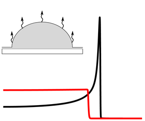
Figure 1. Schematic of an axisymmetric liquid droplet with thickness  $h'(r',t')$ resting on a solid substrate with constant thickness $b'$. The solid is heated to a temperature $T_b$ on its bottom face, and the liquid evaporates with a spatially non-uniform evaporative flux $J'$. The substrate is assumed to be covered by a thin liquid precursor film.
When modelling drying droplets, there are two fundamental complications that arise. The first complication is ameliorating motion of the three-phase contact-line with a no-slip condition at the solid substrate. There are several approaches to this (de Gennes Reference de Gennes1985; Oron, Davis & Bankoff Reference Oron, Davis and Bankoff1997; Kumar & Charitatos Reference Kumar and Charitatos2022), and in the present work we will use a precursor-film approach where the solid substrate is covered by a thin liquid film as depicted in figure 1. This lifts the contact line up from the solid, allowing it to move while still enforcing no-slip conditions at the liquid–solid interface. The liquid pressure is modified to account for van der Waals forces that control droplet spreading and also prevent the precursor film from evaporating. Such films have been observed experimentally (Popescu et al. Reference Popescu, Oshanin, Dietrich and Cazabat2012) and result in governing equations that are easier to solve than those obtained from alternative approaches (Savva & Kalliadasis Reference Savva and Kalliadasis2011). The second complication is modelling the evaporation process, which proceeds through two main steps: liquid first undergoes phase change into vapour and is then transported away from the liquid–gas interface into the surroundings.
Existing models for evaporation are distinguished largely by which of the two steps is assumed to be rate limiting. The two predominant evaporation models are the one-sided model, which assumes that phase change is rate limiting, and the diffusion-limited model, which assumes that diffusive transport of vapour is rate limiting. Both have been used widely in previous work, and their predictions can differ greatly from each other, but fundamental understanding of the physical mechanisms underlying these differences is largely lacking. We seek to develop this understanding in the present work, so we begin with an overview of each evaporation model and its use in previous work.
1.1. One-sided evaporation
The one-sided (or non-equilibrium one-sided) evaporation model assumes that evaporation is rate-limited by the phase change to vapour, and that the liquid is evaporating into its own saturated vapour. One-sided evaporation is driven by deviations from saturated conditions, and its description was pioneered by Schrage (Reference Schrage1953) using the kinetic theory of gases. The term ‘one-sided’ is used because the transport problem in the liquid decouples from that in the gas, and one obtains an analytical expression for the evaporative flux by considering only transport in the liquid (similar to that of a simple mass-transfer coefficient model) (Ajaev Reference Ajaev2005; Parrish & Kumar Reference Parrish and Kumar2020). This is typically done in the context of lubrication theory (thin droplets), yielding an evolution equation without any other assumptions on the droplet shape. Hence the one-sided model is more amenable to describing droplets with asymmetric shapes (Charitatos, Pham & Kumar Reference Charitatos, Pham and Kumar2021; Issakhani et al. Reference Issakhani, Jadidi, Farhadi and Bazargan2023). At its edge, the droplet merges onto a precursor film of constant thickness that does not evaporate away due to the inclusion of disjoining pressure.
Predictions from models using one-sided evaporation agree well with experiments on droplets evaporating in saturated conditions (Sodtke, Ajaev & Stephan Reference Sodtke, Ajaev and Stephan2008), and can fit experimental data even when the gas phase is not saturated vapour (Murisic & Kondic Reference Murisic and Kondic2011). This agreement, along with its simplicity, has led to one-sided evaporation being used in a number of theoretical studies of evaporating droplets as well as films (Burelbach, Bankoff & Davis Reference Burelbach, Bankoff and Davis1988; Oron et al. Reference Oron, Davis and Bankoff1997; Ajaev Reference Ajaev2005; Cazabat & Guéna Reference Cazabat and Guéna2010; Maki & Kumar Reference Maki and Kumar2011; Karapetsas, Sahu & Matar Reference Karapetsas, Sahu and Matar2016; Pham & Kumar Reference Pham and Kumar2017, Reference Pham and Kumar2019; Charitatos & Kumar Reference Charitatos and Kumar2020; Larsson & Kumar Reference Larsson and Kumar2022). Note that because the one-sided evaporation model considers only transport in the liquid, it cannot describe the interactions between multiple droplets via the vapour phase (e.g. shielding effects) (Masoud, Howell & Stone Reference Masoud, Howell and Stone2021; Wray et al. Reference Wray, Wray, Duffy and Wilson2021; Wilson & D'Ambrosio Reference Wilson and D'Ambrosio2022).
1.2. Diffusion-limited evaporation
The diffusion-limited evaporation model assumes that diffusive transport of vapour away from the liquid–gas interface is the rate-limiting step. Furthermore, it assumes that the liquid is in equilibrium with the vapour directly above it, establishing a relation between the thermodynamic states of the liquid and the gas (e.g. the Kelvin equation). Consequently, one must solve transport problems for both the liquid and gas phases that are coupled by the equilibrium condition and evaporative flux at the liquid–gas interface. This coupling makes diffusion-limited evaporation more complicated to implement, in general, than one-sided evaporation.
While diffusion-limited evaporation is often implemented without a precursor film, one can be included. Distinct from one-sided evaporation, the precursor film under diffusion-limited evaporation has a thickness that decays to a non-zero value inversely with distance from the droplet contact line (Eggers & Pismen Reference Eggers and Pismen2010). Note that because the diffusion-limited evaporation model uses information from both the vapour and liquid phases, it can be used to describe interactions between multiple droplets via the vapour phase, unlike the one-sided evaporation model.
If evaporation is slower than the relaxation time of the droplet, then capillary pressure will bring the droplet to a spherical-cap shape. With a spherical-cap droplet, diffusion-limited evaporation yields simple expressions for the evaporative flux and time-evolution of the droplet radius (it is sometimes referred to as the ‘lens’ evaporation model) (Deegan et al. Reference Deegan, Bakajin, Dupont, Huber, Nagel and Witten2000; Hu & Larson Reference Hu and Larson2002; Stauber et al. Reference Stauber, Wilson, Duffy and Sefiane2014; Wilson & D'Ambrosio Reference Wilson and D'Ambrosio2022). These expressions impart a great deal of physical insight that has been leveraged to develop fundamental understanding. For example, one can fit experimental measurements of the droplet radius to simple analytical expressions to obtain estimates of the evaporative flux profile and total evaporation rate (Shahidzadeh-Bonn et al. Reference Shahidzadeh-Bonn, Rafaï, Azouni and Bonn2006). Furthermore, knowledge of the structure of the evaporative flux near the contact line allows one to understand and derive expressions for apparent contact angles and thermal gradients (and thus Marangoni flow) in terms of simple physical parameters (Morris Reference Morris2001; Ristenpart et al. Reference Ristenpart, Kim, Domingues, Wan and Stone2007; Jambon-Puillet et al. Reference Jambon-Puillet, Carrier, Shahidzadeh, Brutin, Eggers and Bonn2018).
Diffusion-limited evaporation often well-approximates evaporation rates observed in simple drying-droplet experiments, so it has been attractive for both experimental and theoretical studies (usually assuming a spherical-cap droplet) (Poulard, Bénichou & Cazabat Reference Poulard, Bénichou and Cazabat2003; Hu & Larson Reference Hu and Larson2006; Shahidzadeh-Bonn et al. Reference Shahidzadeh-Bonn, Rafaï, Azouni and Bonn2006; Ristenpart et al. Reference Ristenpart, Kim, Domingues, Wan and Stone2007; Sefiane, David & Shanahan Reference Sefiane, David and Shanahan2008; Eggers & Pismen Reference Eggers and Pismen2010; Larson Reference Larson2014; Tsoumpas et al. Reference Tsoumpas, Dehaeck, Rednikov and Colinet2015; Diddens et al. Reference Diddens, Kuerten, van der Geld and Wijshoff2017a,b; Karpitschka, Liebig & Riegler Reference Karpitschka, Liebig and Riegler2017; Jambon-Puillet et al. Reference Jambon-Puillet, Carrier, Shahidzadeh, Brutin, Eggers and Bonn2018; Pahlavan et al. Reference Pahlavan, Lisong, Bain and Stone2021; Wray et al. Reference Wray, Wray, Duffy and Wilson2021; Gelderblom, Diddens & Marin Reference Gelderblom, Diddens and Marin2022; Thayyil Raju et al. Reference Thayyil Raju, Diddens, Li, Marin, van der Linden, Zhang and Lohse2022; Yariv Reference Yariv2023) and has also been used to model drying films (Dey, Doumenc & Guerrier Reference Dey, Doumenc and Guerrier2016; Loussert et al. Reference Loussert, Doumenc, Salmon, Nikolayev and Guerrier2017; Sobac, Colinet & Pauchard Reference Sobac, Colinet and Pauchard2019; Larsson & Kumar Reference Larsson and Kumar2022).
1.3. Overview of present paper
While both one-sided and diffusion-limited evaporation have been used widely in previous studies, few have compared them (Sultan, Boudaoud & Ben Amar Reference Sultan, Boudaoud and Ben Amar2005; Murisic & Kondic Reference Murisic and Kondic2011; Moore, Vella & Oliver Reference Moore, Vella and Oliver2021; Hartmann et al. Reference Hartmann, Diddens, Jalaal and Thiele2023). Note that while the physical assumptions made by each model are distinct, it is not always clear which model is appropriate to use to describe a given experiment (Shahidzadeh-Bonn et al. Reference Shahidzadeh-Bonn, Rafaï, Azouni and Bonn2006; Cazabat & Guéna Reference Cazabat and Guéna2010; Murisic & Kondic Reference Murisic and Kondic2011). Most notably, Murisic & Kondic (Reference Murisic and Kondic2011) compared directly one-sided and diffusion-limited evaporation by fitting predictions to experimental data for evaporating sessile droplets. They found that agreement of each model with experiment depended on the physical system (e.g. water versus isopropanol droplets), attributing the differences to inaccurately predicted thermal Marangoni flow. However, it is difficult to extract understanding of the physical mechanisms underlying these different predictions because Murisic & Kondic (Reference Murisic and Kondic2011) assume spherical-cap droplets, do not isolate thermal effects, and fit their model predictions to experimental data with widely varying droplet lifetimes.
Thus, in this work, we will develop this understanding by considering droplets with given lifetimes. We will then show how the two different evaporation models give rise to inaccurately predicted thermal gradients for some physical systems but not others (as observed by Murisic & Kondic Reference Murisic and Kondic2011). To better highlight physical mechanisms, we confine our analysis to the case of isolated droplets with a circular footprint. For the same reason, we treat each evaporation model separately rather than considering more complex evaporation models that can transition between these two limiting cases (Sultan et al. Reference Sultan, Boudaoud and Ben Amar2005).
First, the mathematical model is presented in § 2. Next, in § 3, we highlight a novel hybrid spectral finite-difference method that we have developed to solve the governing equations, and the challenges it overcomes. Because the two models exhibit significant differences in evaporation behaviour, we discuss the droplet-lifetime-matching procedure in § 4. Direct comparisons without thermal effects are given in § 5. In § 6, we show that thermal Marangoni flow is always directed away from the contact line under one-sided evaporation, in contrast to diffusion-limited evaporation, where it is known that the direction depends on the liquid/solid thermal conductivity ratio (Ristenpart et al. Reference Ristenpart, Kim, Domingues, Wan and Stone2007). Conclusions are given in § 7.
2. Mathematical model
We consider a thin, axisymmetric droplet of pure solvent as depicted in figure 1. The droplet height is given by  $h'(r', t')$, where $r'$ is the radial coordinate, and $t'$ is time. The evaporative flux $J'(r',t')$, in general, also varies with space and time.
2.1. Hydrodynamics
The liquid is Newtonian with density  $\rho$, viscosity $\mu$, and surface tension $\sigma '$. The characteristic vertical and lateral length scales of the droplet are given by $H$ and $L$, respectively. Their ratio, $\epsilon =H/L\ll 1$, is assumed small so that lubrication theory may be leveraged. The liquid motion is subject to no-slip and no-penetration conditions at the solid substrate, and stress balances at the liquid–gas interface.
We use the scale  $p^*=\sigma _0\epsilon ^2/H$ for the pressure $p'$,
$p'$,  $v_r^*=\epsilon ^3\sigma _0/\mu$ for the $r$ velocity $v_r'$, $v_z^*=\epsilon v_r^*$ for the $z$ velocity $v_z'$, and $t^*=H/v_r^*\epsilon$ for the time $t'$. These scales are derived from balancing terms in the mass and momentum balances (Larsson & Kumar Reference Larsson and Kumar2021). The quantity $\sigma _0$ is the surface tension at the saturation temperature $T_s$ and is used to scale $\sigma '$. Finally, for the evaporative flux $J'$, we use a general scale $J^*$ (defined in § 2.2) and non-dimensionalize the temperature $T'$ as $T=(T'-T_{s})/(T_b-T_s)$, where $T_b>T_s$ is the temperature of the heated substrate. For the remainder of this work, we use dimensionless variables (indicated without a prime superscript):
 \begin{equation} \left.\begin{gathered} r'=\epsilon^{-1}Hr,\quad z'=Hz,\quad h'=Hh,\quad T'=(T_b-T_s)T+T_{s},\\ v_r' = v_r^*v_r,\quad v_z'=\epsilon v_r^*v_z,\quad p'=p^*p,\quad t'=t^*t,\quad J'=J^*J. \end{gathered}\right\} \end{equation}
Surface tension  $\sigma$ is assumed to vary linearly with the dimensionless interface temperature $T_I=T\vert _{z=h}$:
 \begin{equation} \sigma=1-\epsilon^2\,Ma\,T_I, \end{equation}
where the Marangoni number is  $Ma=(\partial \sigma '/\partial T' )(T_b-T_s)/\sigma _0\epsilon ^2$.
Under the lubrication approximation, the Navier–Stokes equations become
 $$\begin{gather} \frac{\partial^2 v_r}{{\partial z}^2}=\frac{\partial p}{\partial r}, \end{gather}$$
 $$\begin{gather}\frac{\partial p}{\partial z}=0, \end{gather}$$
 $$\begin{gather}\frac{1}{r}\,\frac{\partial}{\partial r}(rv_r)+\frac{\partial v_z}{\partial z}=0, \end{gather}$$
with the boundary conditions  $v_r=v_z=0$ at $z=0$, and
 $$\begin{gather} p=-\frac{1}{r}\,\frac{\partial}{\partial r}\left( r\,\frac{\partial h}{\partial r} \right)-\varPi, \end{gather}$$
 $$\begin{gather}\frac{\partial v_r}{\partial z}=-Ma\,\frac{\partial T_I}{\partial r}, \end{gather}$$
at  $z=h$, where $\varPi$ is the disjoining pressure.
As stated, the no-slip condition imposed at the substrate does not allow for contact-line motion. There are several approaches to ameliorating this, and in this work we use a precursor-film approach because the resulting equations are much easier to solve (Savva & Kalliadasis Reference Savva and Kalliadasis2011; Kumar & Charitatos Reference Kumar and Charitatos2022). It is assumed that the substrate is covered with a thin precursor film and the liquid pressure is modified with a disjoining pressure to account for van der Waals interactions. As in previous work (Schwartz Reference Schwartz1998; Murisic & Kondic Reference Murisic and Kondic2011; Espín & Kumar Reference Espín and Kumar2017; Pham & Kumar Reference Pham and Kumar2017, Reference Pham and Kumar2019; Charitatos & Kumar Reference Charitatos and Kumar2020), we use a two-term disjoining pressure that includes both attractive and repulsive interactions,
 \begin{equation} \varPi(h)=A_1\left( \left( \frac{A_2}{h} \right)^3-\left( \frac{A_2}{h} \right)^2 \right), \end{equation}
where  $A_1$ is a dimensionless Hamaker constant, and $A_2$ controls the thickness at which the disjoining pressure vanishes. The constants $A_1$ and $A_2$ also control the scaled equilibrium contact angle $\theta _{eq}$ through the relation (Schwartz Reference Schwartz1998)
 \begin{equation} \theta_{eq}\approx\sqrt{A_1A_2}. \end{equation}
This is related to the lab-frame contact angle  $\theta _{eq}'$ by $\theta _{eq}'\approx \epsilon \theta _{eq}$. The precursor-film thickness $h_p$ is determined by the condition $J(h_p)=0$, which will be discussed in §§ 2.3.1 and 2.3.2. We have found that using a one-term attractive model for $\varPi$ (corresponding to a perfectly wetting liquid) results in smaller apparent contact angles, but does not change qualitatively the findings presented in this work (Ajaev Reference Ajaev2005; Eggers & Pismen Reference Eggers and Pismen2010; Maki & Kumar Reference Maki and Kumar2011; Karpitschka et al. Reference Karpitschka, Liebig and Riegler2017).
Solving (2.3) and (2.4) subject to boundary conditions (2.6) and (2.7) yields the radial velocity
 \begin{equation} v_r=\left( \frac{1}{2}\,z^2-hz \right)\frac{\partial p}{\partial r}-z\,Ma\,\frac{\partial T_I}{\partial r}. \end{equation}
Finally, mass conservation at the interface  $z=h$ coupled with the continuity equation (2.5) gives the kinematic condition governing the film height:
 \begin{equation} \frac{\partial h}{\partial t}=-\frac{1}{r}\,\frac{\partial}{\partial r}\int_0^hrv_r\,\textrm{d}{z}-EJ=\frac{1}{3r}\,\frac{\partial}{\partial r} \left( rh^3\,\frac{\partial p}{\partial r}\right)+\frac{Ma}{2r}\,\frac{\partial}{\partial r}\left( rh^2\,\frac{\partial T_I}{\partial r}\right)-EJ, \end{equation}
where the pressure  $p$ is given by (2.6), the evaporative number is $E=J^*/\epsilon \rho v_r^*$ (the ratio of evaporative and convective fluxes), and specific expressions for the evaporative flux $J$ will be given in § 2.3. This equation is subject to the symmetric boundary condition $h(r)=h(-r)$ as well as matching onto the precursor film $h\to h_p$ as $r\to \infty$.
2.2. Energy transport
The solid substrate is held at a constant dimensionless temperature  $T=1$ on its bottom face at $z=-b$, where $b=b'/H$ is the thickness of the solid substrate. The solid and liquid have thermal conductivities $k_s$ and $k_\ell$, respectively. Because the droplet is thin, the temperature is governed by
 \begin{equation} \frac{\partial^2 T}{{\partial z}^2}=0 \end{equation}
in both phases, and subject to the boundary conditions
 $$\begin{gather} \left.T\right\vert_{z=-b}=1,\quad \left.T\right\vert_{z=0^-}=\left.T\right\vert_{z=0^+}, \end{gather}$$
 $$\begin{gather}\left.\frac{\partial T}{\partial z}\right\vert_{z=0^-}=\frac{\kappa}{b}\left.\frac{\partial T}{\partial z}\right\vert_{z=0^+},\quad -\left.\frac{\partial T}{\partial z}\right\vert_{z=h}=J, \end{gather}$$
where  $\kappa =bk_\ell /k_s$ is a scaled thermal conductivity ratio, and we use the evaporative flux scale $J^*=\Delta T'\,k_\ell /L_m H$, where $L_m$ is the latent heat of vaporization.
Solving these equations yields the temperature field
 \begin{equation} T = \begin{cases} 1-\kappa J\left( 1+\dfrac{z}{b} \right), & -b \leq z < 0, \\ 1-J\left( z+\kappa \right), & 0 \leq z \leq h. \end{cases} \end{equation}
Of chief concern is the temperature at the liquid–gas interface,
 \begin{equation} T_I=\left.T\right\vert_{z=h}=1-J(h+\kappa), \end{equation}
which depends on the evaporative flux  $J$, the film height $h$, and the conductivity ratio $\kappa$.
2.3. Evaporation
We now present expressions for the evaporative flux  $J$ that appears in (2.11) and (2.16) for both one-sided and diffusion-limited evaporation.
2.3.1. One-sided evaporation
The one-sided evaporation model gives a constitutive relation for the evaporative flux  $J$, which is (in non-dimensional form) (Burelbach et al. Reference Burelbach, Bankoff and Davis1988; Ajaev Reference Ajaev2005)
 \begin{equation} KJ=\delta p+T_I, \end{equation}
where
 \begin{equation} K=\frac{k_\ell\sqrt{2{\rm \pi} R_gT_s^3}}{\rho_vL_m^2\alpha H},\quad \delta=\frac{p^*T_s}{\rho L_m\,\Delta T}. \end{equation}
Here,  $R_g$ is the specific gas constant, $\rho _v$ is the density of the vapour, and $\alpha$ is the accommodation coefficient. The parameter $K$ gives a measure of kinetic effects and the volatility of the liquid, and can be interpreted as the inverse of an effective mass-transfer coefficient (Ajaev Reference Ajaev2005; Parrish & Kumar Reference Parrish and Kumar2020). The parameter $\delta$ measures the effect of changes in local pressure on the phase-change temperature (Ajaev Reference Ajaev2005). Substituting (2.16) into (2.17) yields the one-sided evaporative flux
 \begin{equation} J=\frac{1+\delta p}{K+h+\kappa}, \end{equation}
which is an explicit, local function of the film height  $h$.
$h$.
The precursor-film thickness  $h_p$ is determined by the condition $J=0$ for a flat film. With the pressure given by (2.6), (2.19) reduces to finding the roots of a cubic polynomial:
 \begin{equation} 0=1+\delta p=1-\delta\,\varPi(h_p) \quad\Rightarrow\quad 0=h_p^3+\delta A_1A_2^2h_p-\delta A_1A_2^3. \end{equation}
The discriminant of this polynomial is negative, thus the single real root is
 \begin{equation} h_p=2A_2\sqrt{\frac{\delta A_1}{3}}\sinh\left[ \frac{1}{3}\ \text{asinh} \left(\frac{3}{2}\sqrt{\frac{3}{\delta A_1}} \right)\right], \end{equation}
where  $\sinh$ is the hyperbolic sine function, and $\textrm {asinh}$ is its inverse. This relation is used to determine the precursor-film thickness in the initial condition to the numerical method described in § 3 when using one-sided evaporation.
2.3.2. Diffusion-limited evaporation
Under diffusion-limited evaporation, the evaporative flux  $J$ is determined by the diffusive flux of vapour at the liquid–gas interface $z=h$. It has been shown that in many scenarios, transient effects as well as convection are negligible in the gas phase (Larson Reference Larson2014), so the transport problem reduces to pseudo-steady-state diffusion. The droplet interface is assumed to be in thermodynamic equilibrium, allowing us to relate the thermodynamic states of the liquid and gas phases.
Figure 2 depicts the problem for the dimensionless gas-phase concentration  $c_g$ above the droplet. We use the vertical coordinate $z^*=z'/L$ since there is no apparent vertical scale (unlike inside the droplet), and $c_g$ is defined on the semi-infinite domain $z^*\in (\epsilon h, \infty )$ and $r\in (0,\infty )$. Because the droplet is thin and $\epsilon h\ll 1$, we can neglect the droplet height and instead use the constant domain $z^*\in (0,\infty )$ (shown formally in Appendix A). It is assumed that the vapour is at an ambient concentration $c_\infty$ far from the droplet, so we non-dimensionalize $c_g'$ as $c_g=(c_g'-c_\infty ')/c_{s}$, where $c_s$ is the concentration of saturated vapour. We then have $c_g\to 0$ as $r\to \infty$ or $z^*\to \infty$, as shown in figure 2.

Figure 2. Schematic of the vapour concentration  $c_g$ problem in the semi-infinite domain $r\in (0,\infty )$ and $z^*\in (0,\infty )$. The thin liquid droplet (and precursor film) is in thermodynamic equilibrium with the vapour phase, so we use the Kelvin equation to describe $c_g$ at $z^*=0$.
The governing equation for  $c_g$ is
 \begin{equation} 0=\nabla^2c_g=\frac{\partial^2 c_g}{{\partial z^*}^2}+\frac{1}{r}\,\frac{\partial}{\partial r}\left( r\,\frac{\partial c_g}{\partial r} \right). \end{equation}
For boundary conditions in  $r$, we have the symmetric condition $c_g(r)=c_g(-r)$, which implies that $\partial c_g/\partial r$ and ${\partial ^3 c_g}/{\partial r^3}$ vanish at $r=0$. We also enforce matching to the ambient concentration $c_g\to 0$ as $r\to \infty$. In $z^*$, we match to the ambient concentration as $z^*\to \infty$ and then enforce thermodynamic equilibrium with the liquid droplet at $z^*=0$. For this, we use the Kelvin equation, which accounts for the effect of interface curvature and disjoining pressure on thermodynamic equilibrium (Eggers & Pismen Reference Eggers and Pismen2010):
 \begin{equation} \left.c_g\right\vert_{z^*=0}={\rm e}^{Zp}-c_\infty, \end{equation}
where  $c_\infty = c_\infty '/c_s<1$, $Z=Mp^*/\rho R_g^* T$ is an effective compressibility factor, $M$ is the molecular weight of the liquid, and $R_g^*$ is the universal gas constant. If $Z=0$, then we obtain $c_g\vert _{z^*=0}=1-c_\infty$, or in dimensional terms, $c_g'\vert _{z^*=0}=c_s$, which is consistent with the classical diffusion-limited evaporation model. However, note that the term $Zp$ in (2.23) is never negligible in the precursor film due to large disjoining pressures (see (2.6) and (2.8)) that prevent the film from evaporating away. Later, we will adjust the values of $c_\infty$ and $Z$ to match the droplet lifetime with that from one-sided evaporation.
To obtain the evaporative flux  $J$, we employ Fick's law so that
 \begin{equation} J=-\frac{J_D^*}{J^*}\left.\frac{\partial c_g}{\partial z^*}\right\vert_{z^*=0}, \end{equation}
where  $J_D^*=c_s D\epsilon /H$ is the evaporative-flux scale arising from diffusion (opposed to $J^*$ from energetic considerations), and $D$ is the diffusivity of the vapour. For the purpose of this work, we assume the ratio $J_D^*/J^*$ to be near unity and neglect it, but in practice it may be absorbed into the evaporative number $E$ without loss of generality. A noteworthy result is the analytical solution for $J$ developed by Eggers & Pismen (Reference Eggers and Pismen2010); considering a problem analogous to that shown in figure 2, they showed that (in the current notation)
 \begin{equation} J(r)=-\int_0^\infty\mathcal{K}(r,r')\,\frac{\partial c_g\vert_{z^*=0}}{\partial r'}\,\textrm{d}{r'}, \end{equation}
where the kernel  $\mathcal {K}$ involves the complete elliptic integrals of the first and second kind. As will be discussed in § 3, we have found numerical solution of (2.22) and (2.24) to be more stable in our nonlinear simulations, but the analytical results encapsulated in (2.25) offer valuable insight into the behaviour of $c_g$ and $J$, and will be leveraged in § 3. Furthermore, (2.25) demonstrates that $J$ is a global function of $h$ – distinct from the local function of $h$ obtained under one-sided evaporation (2.19).
The precursor-film thickness  $h_p$ is determined by $J=0$, which is equivalent to $(\partial c_g/\partial z^*)\vert _{z^*=0}=0$ by (2.24). For a flat film at steady state (e.g. a precursor film), (2.22) implies that $c_g$ depends linearly on $z^*$. Since $c_g$ vanishes far from the film, and since the first derivative of $c_g$ vanishes at the film surface, $c_g=0$ everywhere for a flat film at steady state. Equation (2.23) then yields the cubic equation
 \begin{equation} 0=h_p^3+\frac{ZA_1A_2^2}{-\ln c_\infty}\,h_p-\frac{ZA_1A_2^3}{-\ln c_\infty}, \end{equation}
which is equivalent to (2.20) with  $\delta$ replaced by $Z/(-\ln c_\infty )$ (note that $c_\infty <1$). Thus through the same method employed to obtain (2.21), we obtain
 \begin{equation} h_p=2A_2\sqrt{\frac{ZA_1}{-3\ln c_\infty}}\sinh\left[ \frac{1}{3}\ \text{asinh} \left( \frac{3}{2}\sqrt{-\frac{3\ln c_\infty}{ZA_1}} \right) \right]. \end{equation}
This relation is used to determine the precursor-film thickness in the initial condition to the numerical method described in § 3 when using diffusion-limited evaporation.
2.4. Parameter values
The effects of the key dimensionless groups shown in table 1 will be investigated in §§ 5 and 6. The remaining parameters –  $A_1$ and $A_2$ for the disjoining pressure, $\delta$ and $K$ for one-sided evaporation, and $Z$ and $c_\infty$ for diffusion-limited evaporation – are fixed for the remainder of this work. The constants $A_1=10^2$ and $A_2=10^{-3}$ are chosen close to those used in previous work (Pham & Kumar Reference Pham and Kumar2017; Charitatos et al. Reference Charitatos, Pham and Kumar2021) and give a scaled equilibrium contact angle $\theta _{eq}\approx 18^\circ$ (see (2.9)). Following Murisic & Kondic (Reference Murisic and Kondic2011), we choose $K=10$ and $\delta =10^{-3}$ (determined by fitting predictions to experimental measurements of evaporating water droplets), giving $h_p\approx 3.9\times 10^{-4}$. As will be discussed in § 4, we choose $Z=7.69\times 10^{-5}$ and $c_\infty =9.26\times 10^{-1}$ to match the total evaporation time as well as $h_p$ under diffusion-limited evaporation. Note that at this small value of $Z$, the vapour concentration is very nearly constant over the droplet surface as discussed in § 2.3.2.
Table 1. Important dimensionless parameters and typical values.

3. Numerical method
Equations (2.11) and (2.22) are solved numerically from the initial condition
 \begin{equation} h(t=0,r)=\begin{cases} h_p+\left( h_0-h_p \right)\left( 1-\left(\dfrac{r}{R_0}\right)^2 \right), & r \leq R_0, \\ h_p, & r > R_0, \end{cases} \end{equation}
which represents an initially parabolic droplet with height  $h_0$ and radius $R_0$. In this work, we fix $h_0=2$ and $R_0=1$ since the droplet relaxes rapidly to an equilibrium shape before significant evaporation occurs. Even though the initial condition has discontinuous slope, it is smoothed out quickly in the simulations. For (2.11) (excepting the evaporative flux $J$), we use a second-order centred finite-difference method (Diez & Kondic Reference Diez and Kondic2002). To compute $J$ under each evaporation model, we use the methods described in §§ 3.1 and 3.2.
3.1. One-sided evaporative flux
Under one-sided evaporation,  $J$ given by (2.19) is an explicit, local function of the liquid thickness $h$ and is thus easily computed alongside the finite-difference method used to solve (2.11). There are no additional numerics required.
3.2. Diffusion-limited evaporative flux
Under diffusion-limited evaporation,  $J$ is obtained from the solution of (2.22) and is thus an implicit, global function of $h$ (see (2.25)). When approached numerically, commonly (2.22) is solved with a finite-element method (Diddens Reference Diddens2017; Diddens et al. Reference Diddens, Kuerten, van der Geld and Wijshoff2017a; Pahlavan et al. Reference Pahlavan, Lisong, Bain and Stone2021; Thayyil Raju et al. Reference Thayyil Raju, Diddens, Li, Marin, van der Linden, Zhang and Lohse2022), but many analytical simplifications have been developed. Eggers & Pismen (Reference Eggers and Pismen2010) derived (2.25), which removes the necessity of solving a partial differential equation (PDE) at each time step. However, the kernel $\mathcal {K}$ is ill-conditioned and singular at $r'=r$, so computation of the integral is numerically complex and prone to error that can induce instability in the time-stepping algorithm. An alternative is to assume that the droplet is a spherical cap, in which case the evaporative flux is given by
 \begin{equation} J= \frac{2}{\rm \pi}\,\frac{1-c_\infty}{\sqrt{R^2-r^2}}, \end{equation}
which removes any numerical complications when computing the evaporative flux (note that a similar approximation can also used for non-thin droplets) (Wilson & D'Ambrosio Reference Wilson and D'Ambrosio2022). Equation (3.2) is simple and useful for gaining physical insight, so we will reference it when discussing our results. However, we seek to develop understanding for more general droplet shapes, so to compute  $J$ in our nonlinear simulations, we solve (2.22) using the novel hybrid spectral finite-difference method detailed below.
Since the value of  $h$ is required in the equilibrium boundary condition for $c_g$ (2.23), it is convenient to choose the same discretization for $r$ for both (2.11) and (2.22) (second-order centred finite differences). This necessitates a finite $r$ domain despite the boundary conditions for (2.22) as $r\to \infty$. It has been shown that, away from the contact line, $h$ decays to the precursor-film thickness as $1/r$ (Eggers & Pismen Reference Eggers and Pismen2010), so an $r$ domain that is significantly larger than the droplet radius is required to resolve the evaporative flux properly. We choose $r\in (0,100)$ because scaling relations (Eggers & Pismen Reference Eggers and Pismen2010), as well as numerical results from our simulations, show that this is adequate to resolve the evaporative flux within numerical tolerances.
We must also discretize (2.22) in the  $z^*$ domain. It is possible to similarly choose a finite distance (Diddens Reference Diddens2017; Loussert et al. Reference Loussert, Doumenc, Salmon, Nikolayev and Guerrier2017) and solve in a truncated $z^*$ domain by finite elements or finite differences. However, unlike the $r$ domain, the proper distance in the $z^*$ domain is unclear. Furthermore, we are not restrained by boundary data as in the $r$ domain, so it is possible to use a different discretization that is capable of resolving semi-infinite domains. Thus we use a spectral method in $z^*$ with Laguerre basis functions on the domain $z^*\in (0,\infty )$. The Laguerre functions (Boyd Reference Boyd2001) $L_n(z^*)$ are a modification of the Laguerre polynomials (Abramowitz & Stegun Reference Abramowitz and Stegun1964) $\ell _n(z^*)$ to a semi-infinite domain:
 \begin{equation} L_n(z^*)=\exp({-z^*/2})\,\ell_n(z^*). \end{equation}
We choose these basis functions over other candidates because they decay exponentially, which matches the exponential decay of  $c_g$ shown by Eggers & Pismen (Reference Eggers and Pismen2010).
This hybrid spectral finite-difference method represents the gas-phase concentration as the expansion
 \begin{equation} c_g(r,z^*,t)\approx\sum_{n=0}^{M-1}a_n(r,t)\,L_n(z^*), \end{equation}
where the coefficients  $a_n$ depend on $r$ and $t$. Inserting this into (2.22) and applying orthogonality of the Laguerre functions gives the PDE
 \begin{equation} a_n''+\frac{1}{r}\,\frac{\partial}{\partial r}\left( r\,\frac{\partial a_n}{\partial r} \right)=0, \end{equation}
for each  $n$, where $a_n''(a_1,\ldots,a_{n})$ gives the coefficients of the second $z^*$ derivative of $c_g$. This PDE can be discretized further in $r$ with the same finite-difference method, and solved for $a_n$ alongside (2.11). The evaporative flux is then obtained from the relation
 \begin{equation} J(r,t)=-\sum_{n=0}^{M-1}a_n'(r,t), \end{equation}
which follows from the identity  $L_n(0)=1$. Here, $a_n'$ are the coefficients of the first $z^*$ derivative of $c_g$.
The end result of this numerical method is the reduction of (2.22) to an  $NM\times NM$ banded system of equations with bandwidth $4M$, where $M$ is the number of Laguerre functions, and $N$ is the number of finite-difference cells, that is solved efficiently by standard banded-system solvers. This requires computational time and memory similar to a full finite-difference/element method, but is capable of resolving the entire semi-infinite domain with spectral accuracy in $z^*$. To the best of our knowledge, this is the first numerical method to employ Laguerre functions in the context of evaporation. See the supplementary material available at https://doi.org/10.1017/jfm.2023.873 for a detailed discussion of implementing this method.
For accuracy, we must have high resolution near the droplet contact line. However, this level of resolution is not necessary far from the droplet. Thus, near the droplet, we use cells with constant width, but those far from the droplet become wider. Formally, the cells at a radius less than a critical radius,  $r< r_c$, have constant width, and each cell beyond $r_c$ is a factor $c$ wider than the previous one. For a given number of nodes $N$, the number of nodes inside the critical radius $N_i$ is given by
 \begin{equation} N_i=-\alpha+\frac{1}{\ln c}\,{W}(\alpha c^{N+\alpha}\ln c), \end{equation}
where  $\alpha =cr_c/(c-1)(d-r_c)$, $d$ is the size of the $r$ domain, and $W$ is the principal branch of the Lambert- $W$ function (Corless et al. Reference Corless, Gonnet, Hare, Jeffrey and Knuth1996). In this work, we use $r_c=2$, $c=1.05$, $d=100$ and $N=4000$ nodes, giving $N_i\approx 3807$. This approach covers the entire domain $r\in (0,100)$ with only minor cell stretching, while placing over $95\,\%$ of the cells near or inside the droplet ( $r<2$).
This hybrid spectral finite-difference method also allows computation of the vapour field  $c_g$ above the droplet, whereas direct expressions for $J$ such as (2.25) and (3.2) provide no information about $c_g$. Figure 3 shows $c_g$ above a droplet with radius $R\approx 1.4$ (located at $z^*=0$) where we present $z^*$ on a logarithmic scale to show that the vapour concentration $c_g$ decays exponentially. Vapour is concentrated near the droplet at $z^*=0$ and approaches the scaled ambient value $c_g=0$ as $z^*\to \infty$ or $r\to \infty$. Note that establishing this vapour field is critical to the diffusion-limited evaporation model; processes such as convection can interfere and cause the diffusion-limited model to become inaccurate (Shahidzadeh-Bonn et al. Reference Shahidzadeh-Bonn, Rafaï, Azouni and Bonn2006). As will be discussed in § 5, one-sided evaporation may offer a more accurate description in such a scenario.

Figure 3. (a) Example of the vapour concentration  $c_g$ above the droplet (located at $z^*=0$). (b) Plots of the vapour concentration $c_g$ at fixed $r$. Straight dashed lines are provided for reference to show that $c_g$ decays exponentially ( $\ln c_g\sim z^*$) for sufficiently large $z^*$.
4. Evaporation time matching
In this section, we develop expressions for the droplet lifetime under diffusion-limited and one-sided evaporation. By equating these expressions, we obtain relations between parameters that ensure a consistent droplet lifetime between the two evaporation models.
To begin, we integrate (2.11) over the droplet radius to obtain
 \begin{equation} \frac{{\rm d}}{{\rm d} t}\int_0^R rh\,\textrm{d}{r}=-E\int_0^R rJ\,\textrm{d}{r}. \end{equation}
Note that this equation is simply conservation of volume, balancing the change in droplet volume with the total evaporation rate. For simplicity, we assume in this derivation that the droplet shape is given by the lubrication limit of a spherical cap,
 \begin{equation} h(r,t) = \frac{R(t)}{2}\tan\theta_a\left( 1-\left(\frac{r}{R(t)}\right)^2 \right), \end{equation}
where  $\theta _a$ is the apparent contact angle (assumed constant). While technically this is a parabola, we will refer to it as a spherical-cap shape for simplicity. We then have the volume change
 \begin{equation} \frac{{\rm d}}{{\rm d} t}\int_0^R rh\,\textrm{d}{r}=\frac{3}{8}\,R^2\tan\theta_a\,\frac{{\rm d} R}{{\rm d} t}. \end{equation}
Under diffusion-limited evaporation with a spherical-cap droplet, we have
 \begin{equation} J_{tot}=\int_0^R rJ\,\textrm{d}{r}=\frac{2(1-c_\infty)}{\rm \pi} \int_0^R\frac{r}{\sqrt{R^2-r^2}}\,\textrm{d}{r}=\frac{2}{\rm \pi}\,R(1- c_\infty), \end{equation}
where we substituted (3.2) for  $J$. It is known that the total evaporation rate for diffusion-limited evaporation is proportional to the droplet radius (Shahidzadeh-Bonn et al. Reference Shahidzadeh-Bonn, Rafaï, Azouni and Bonn2006; Wilson & D'Ambrosio Reference Wilson and D'Ambrosio2022); here, we see that the constant of proportionality is $2(1-c_\infty )/{\rm \pi}$ in (4.4). Inserting (4.3) and (4.4) into (4.1) and integrating gives the relation
 \begin{equation} R(t)=\sqrt{C_d\left(t_0^{(d)}-t\right)}, \end{equation}
where  $C_d=32E(1-c_\infty )/3{\rm \pi} \tan \theta _a$, and $t_0^{(d)}$ is the droplet lifetime for diffusion-limited evaporation ( $R(t_0^{(d)})=0$). With an initial radius $R_i=R(t=0)$, we can solve for $t_0^{(d)}$:
 \begin{equation} t_0^{(d)}=\frac{R_i^2}{C_d}=\frac{3{\rm \pi}}{32}\,\frac{R_i^2\tan\theta_a}{E(1-c_\infty)}. \end{equation}
When dimensionalized (accounting for the factor  $J^*_D/J^*$ discussed in § 2.3.2), this expression is equivalent to that shown in Wilson & D'Ambrosio (Reference Wilson and D'Ambrosio2022).
Under one-sided evaporation, with (4.2) for  $h$, we have the total evaporation rate
 \begin{equation} J_{tot}=\int_0^R rJ\,\textrm{d}{r}=\int_0^R\frac{r}{K+h+\kappa}\,\textrm{d}{r}=\frac{R}{\tan\theta_a} \ln\left( 1+\frac{R\tan\theta_a}{2\left( K+\kappa \right)}\right), \end{equation}
where we have neglected the pressure contribution  $\delta p$ in (2.19) for $J$. In addition to allowing us to make analytical progress, this is a physically reasonable approximation since $p\sim 1$ in the bulk of the droplet due to our use of a capillary scale, and with $\delta \ll 1$ as described in § 2.4, the term $\delta p\ll 1$ is negligible in the bulk of the droplet. Substituting (4.3) and (4.7) into (4.1) and integrating gives the relation
 \begin{equation} {li}(\left( 1+\varGamma \right)^2)-{li} \left( 1+\varGamma \right)-\ln 2=\frac{2E}{3(K+\kappa)^2}\,(t_0^{(o)}-t), \end{equation}
where  $li$ is the logarithmic integral function (Abramowitz & Stegun Reference Abramowitz and Stegun1964), $\varGamma =R\tan \theta _a/2(K+\kappa )$, and $t_0^{(o)}$ is the droplet lifetime under one-sided evaporation. While this expression is complicated and implicit in the droplet radius $R$, it will be shown in § 5 that with $\varGamma \ll 1$, it reduces to a linear dependence $R\sim t_0^{(o)}-t$. We note that if additional assumptions are made, then an expression for the droplet lifetime under one-sided evaporation can be obtained using the method of matched asymptotic expansions ((4.2) in Savva, Rednikov & Colinet Reference Savva, Rednikov and Colinet2017).
By equating  $t_0^{(d)}$ from (4.6) and $t_0^{(o)}$ from (4.8), we obtain an expression for $c_\infty$ in terms of parameters from the one-sided evaporation model:
 \begin{equation} \frac{1}{1- c_\infty}=\frac{4}{\rm \pi}\,\frac{\tan\theta_a}{\varGamma_i^2} [{li}((1+\varGamma_i)^2)-{li}(1+\varGamma_i)-\ln 2], \end{equation}
where  $\varGamma _i=R_i\tan \theta _a/2(K+\kappa )$. Note that this assumes a spherical-cap droplet and constant $\theta _a$. Furthermore, $c_\infty$ from (4.9) depends on the initial radius of the droplet $R_i$ since the two evaporation models have different dependencies on the droplet radius, (4.4) and (4.7). Relation (4.9) thus serves as starting point for time matching, where given $K$,
$K$,  $R_i$ and an approximate $\theta _a$ (e.g. from numerical results), an initial estimate for $c_\infty$ can be obtained. The parameter $Z$ (see (2.23)) is then obtained from the relation
 \begin{equation} Z=-\delta\ln c_\infty \end{equation}
that ensures (2.21) and (2.27) yield the same precursor-film thickness  $h_p$.
As discussed in § 2.4, all results presented use  $K=10$ and $\delta =10^{-3}$, which were found by Murisic & Kondic (Reference Murisic and Kondic2011) to well-approximate evaporating water droplets. Using $E=10^{-2}$, these parameters result in an evaporation time $t_0^{(o)}\approx 630$ in the nonlinear simulations with one-sided evaporation. From (4.9) and (4.10), we then obtain $c_\infty \approx 9.38\times 10^{-1}$ and $Z\approx 6.4\times 10^{-5}$ for diffusion-limited evaporation. While close, these parameters do not give exactly the same evaporation time due to the assumptions used to obtain (4.9) and (4.10). Thus we iteratively adjust $c_\infty$ and $Z$ from the initial guess provided by (4.9) and (4.10) until we obtain $t_0^{(d)}\approx t_0^{(o)}\approx 630$; we found that $c_\infty =9.26\times 10^{-3}$ with $Z\approx 7.69\times 10^{-5}$ achieves this. Remarkably, the value of $c_\infty$ predicted by (4.9) was within $1\,\%$ of the value required for time-matching in the full nonlinear simulations.
Because we are concerned with comparing one-sided and diffusion-limited evaporation, and not the specific behaviour of a single model, we do not present the effects of varying  $K$,
$K$,  $\delta$, $Z$ or $c_\infty$ in this work. They do not change qualitatively the comparisons presented in §§ 5 and 6, and many studies have investigated each model in isolation (see the discussion in § 1). However, we will investigate the effect of varying $E$ in § 5 because it accentuates the models’ fundamental differences.
5. Comparison of droplet radius and contact angle
In this section, we make direct comparisons between predictions of the droplet radius and contact angle under one-sided and diffusion-limited evaporation. We begin by discussing the main qualitative features of predictions from each evaporation model. Figure 4(a) shows an example of the droplet height evolution under diffusion-limited evaporation; the droplet spreads out rapidly from the initial radius  $R_0=1$ (not shown) and then begins to retract as evaporation proceeds. The droplet profile under one-sided evaporation is similar, qualitatively. Figure 4(b) shows the evaporative flux $J$ halfway through the droplet lifetime, $t=t_0/2$, for both one-sided and diffusion-limited evaporation. Note that the one-sided evaporative flux (red line) is nearly constant throughout the droplet and decays rapidly to $J=0$ at the contact line. The diffusion-limited evaporative flux (black line) varies more throughout the droplet, resembling the spherical cap solution given by (3.2) (though not singular due to the precursor film). It increases rapidly near the contact line before decaying to $J=0$ in the precursor film.

Figure 4. (a) Droplet shape sampled at intervals of  $t_0/5$ under diffusion-limited evaporation, starting from $t=t_0/10$, where $t_0$ is the droplet lifetime. The arrow points in the direction of increasing time. The evolution is qualitatively similar under one-sided evaporation. (b) The evaporative flux $J$ for both evaporation models at $t=t_0/2$. Note that the droplet radius is larger under diffusion-limited evaporation, despite the same $t_0$, due to different dependencies on the droplet radius (see (4.4) and (4.7)).
The diffusion-limited evaporative flux shown in figure 4(b) (black line) is similar to what has been reported in previous studies. Note, however, that qualitatively different profiles can be obtained, such as a nearly constant profile for droplets resting on hydrogels (Boulogne, Ingremeau & Stone Reference Boulogne, Ingremeau and Stone2016). For one-sided evaporation, the qualitative shape of the evaporative flux (red line) changes depending on the value of the parameter  $K$ in (2.19). When $K\gg h$, the evaporative flux is insensitive to the droplet profile, and $J\approx K^{-1}$ is nearly constant throughout the droplet. However, if $K\sim h$ or $K\ll h$, then $J$ will increase as the droplet thins near the contact line, and the one-sided evaporative flux will resemble qualitatively the diffusion-limited evaporative flux (see Ajaev Reference Ajaev2005; Pham & Kumar Reference Pham and Kumar2017). Thus the evaporative flux is not always nearly constant under one-sided evaporation. In this work, we focus on the case where $K\gg h$ since this is the parameter regime investigated by Murisic & Kondic (Reference Murisic and Kondic2011) and also allows an insightful analytical simplification that will be discussed in § 5.1. Furthermore, the value of $K$ does not affect the qualitative behaviour of the temperature profiles that we investigate in § 6.
Figure 5 shows the droplet radius  $R$ and apparent contact angle $\theta _a$ versus time for both evaporation models. Under diffusion-limited evaporation (black lines), the droplet radius (figure 5a) is well-approximated by (4.5) (dashed line) which shows the expected scaling $R\sim \sqrt {t_0-t}$, and the apparent contact angle (figure 5b) remains nearly constant throughout most of the droplet lifetime. This behaviour of the radius and contact angle has been observed in previous experimental studies (Shahidzadeh-Bonn et al. Reference Shahidzadeh-Bonn, Rafaï, Azouni and Bonn2006; Sefiane et al. Reference Sefiane, David and Shanahan2008). However, under one-sided evaporation (red lines), the radius shrinks almost linearly with time (figure 5a), and the apparent contact angle decreases noticeably over time (figure 5b), which is qualitatively distinct from the behaviour under diffusion-limited evaporation. Note that in the analysis below, we will disregard the initial spreading phase (giving the initial increase in $R$ and decrease in $\theta _a$) as well as the end of the droplet lifetime where the droplet is small enough so that the bulk is no longer distinct from the contact-line region (resulting in another decrease in $\theta _a$).

Figure 5. (a) Radius  $R$ and (b) apparent contact angle $\theta _a$ over time for both evaporation models. Analytical approximations given by (4.5) (black) and (5.3) (red) are plotted as dashed lines in (a). Note that they do not capture the initial spreading phase of the droplet. The apparent contact angle $\theta _a$ is computed from the maximum slope of the liquid–gas interface.
5.1. Comparison of droplet radius
We now compare the two evaporation models to understand the differences in the predictions of the droplet radius. Turning first to diffusion-limited evaporation, the droplet radius shown in figure 5(a) (black lines) is well-approximated by (4.5) because the droplet shape is well-approximated by a spherical cap. Note that this results in (4.4) for the total evaporative flux  $J_{tot}\sim R$ which scales with the droplet circumference. This result holds regardless of the parameters $c_\infty$ and $Z$ as long as the droplet shape is well-approximated by a spherical cap. For other situations, such as those where gravity is important, this approximation may not hold. Note that the nonlinear simulations are not restricted to the case of spherical-cap droplets.
Now focusing on one-sided evaporation and assuming a spherical-cap shape (4.2), we may rewrite  $J$ given by (2.19) in terms of $\varGamma$ (neglecting the pressure contribution because it is unimportant in the bulk):
 \begin{equation} J=\frac{\left(K+\kappa\right)^{-1}}{1+\varGamma\left( 1-\left( \dfrac{r}{R} \right)^2 \right)}. \end{equation}
In the limit that  $\varGamma =R\tan \theta _a/2(K+\kappa )\ll 1$, this reduces to the constant evaporative flux $J\approx ( K+\kappa )^{-1}$. The total evaporative flux then becomes
 \begin{equation} J_{tot}=\int_0^R rJ\,\textrm{d}{r}\approx\frac{R^2}{2(K+\kappa)}. \end{equation}
The condition  $\varGamma \ll 1$ states that the droplet shape does not influence the evaporative flux, hence giving a nearly constant $J$ throughout the bulk. In contrast to the simple analytical relations that one obtains for diffusion-limited evaporation (4.4), (5.2) is valid only in parameter regimes where $\varGamma \ll 1$.
With  $R\sim 1$, $\theta _a\approx 23^\circ$ and $K+\kappa =10$, we have $\varGamma \ll 1$ for results presented in this work – as evidenced by the nearly constant one-sided evaporative flux in figure 4(b). Substituting (5.2) into (4.1) results in a linear scaling for the droplet radius under one-sided evaporation:
 \begin{equation} R(t)=\frac{4E}{3\tan\theta_a(K+\kappa)}\,(t_0^{(o)}-t). \end{equation}
Note that this assumes a constant apparent contact angle  $\theta _a$, and despite $\theta _a$ varying as shown in figure 5(b), well-approximates the radius evolution shown in figure 5(a) (red lines). Equivalently, (5.3) can be obtained by simplifying (4.8) in the limit $\varGamma \ll 1$. We note that a similar linear relationship can be derived for non-thin droplets undergoing constant evaporation (Masoud & Felske Reference Masoud and Felske2009).
In experimental studies of drying droplets, it has been observed that  $J_{tot}$ is proportional to the surface area ( ${\sim }R^2$) in some systems (such as forced convection over the droplet) (Shahidzadeh-Bonn et al. Reference Shahidzadeh-Bonn, Rafaï, Azouni and Bonn2006), and diffusion-limited evaporation fails to capture the evolution because it predicts $J_{tot}$ proportional to the circumference of the droplet ( $J_{tot}\sim R$ as shown in (4.4)). In such a scenario, one-sided evaporation may be able to capture the droplet evolution since it predicts $J_{tot}\sim R^2$ when $\varGamma \ll 1$; by treating the value of $K$ in relations (5.2) and (5.3) as a fitting parameter, one can adjust the evaporation rate to fit experimental data.
5.2. Comparison of droplet contact angle
We now discuss trends in the apparent contact angle  $\theta _a$ and elucidate fundamental differences in the structure of the two evaporation models near the droplet contact line. Figure 5(b) shows that after the initial spreading phase, $\theta _a$ remains nearly constant under diffusion-limited evaporation (black line) but decreases steadily under one-sided evaporation (red line). To understand this difference, we must look more closely at the dynamics near the droplet contact line that give rise to $\theta _a$. Figure 6 shows a scaled-up view of the droplet contact line, where capillary effects tend to spread the droplet while evaporation tends to contract it. Eggers & Pismen (Reference Eggers and Pismen2010) showed that under diffusion-limited evaporation, the size of the contact-line region $w$ scales as $w\sim R^{1/3}$, so $\xi$ depicted in figure 6 is a scaled distance away from the contact line such that $\xi \sim 1$ in the contact-line region:
 \begin{equation} \xi\sim\frac{R-r}{R^{1/3}}. \end{equation}


The driving force for spreading arises from the difference in capillary pressure in the bulk and disjoining pressure in the precursor film. For a spherical-cap droplet, substituting (4.2) into (2.6) (and neglecting disjoining pressure in the bulk) gives
 \begin{equation} p\approx-\frac{1}{r}\,\frac{\partial}{\partial r}\left( r\,\frac{\partial h}{\partial r} \right)=\frac{2\tan\theta_a}{R(t)}. \end{equation}
While the pressure in the precursor film  $p=-\varPi (h_p)$ remains constant and negative, the bulk pressure scales as $p\sim R^{-1}$, which grows as the droplet shrinks. Thus the driving force for spreading becomes larger as the droplet evaporates, which tends to decrease $\theta _a$ over time.
Opposing this capillary spreading is evaporation, where a non-uniform evaporative flux that is focused at the contact line will tend to increase  $\theta _a$. Under diffusion-limited evaporation (assuming a spherical cap for simplicity), we can use (3.2) and (5.4) to show that near the contact line
 \begin{equation} J\sim\frac{1}{\sqrt{R^2-r^2}}\sim\frac{1}{\sqrt{R(R-r)}}\sim\frac{1}{R^{2/3}\sqrt{\xi}}. \end{equation}
First, we see that  $J$ grows like the classical square-root singularity (Eggers & Pismen Reference Eggers and Pismen2010) $\xi ^{-1/2}$ as we move towards the contact line ( $\xi \to 0$), obtaining its maximum (singular) value at $r=R$. Second, note that as the droplet shrinks and $R$ decreases, $J$ increases and becomes more non-uniform (the peak shown in figure 4(b) becomes steeper). Thus diffusion-limited evaporation tends to increase $\theta _a$ as the droplet shrinks, balancing the increasing capillary pressure and giving the nearly constant $\theta _a$ shown in figure 5(b) (black line).
For one-sided evaporation, note that near the contact line we have  $h\approx h_p$, and the pressure is dominated by the disjoining pressure, so we have from (2.19) that
 \begin{equation} J=\frac{1+\delta p}{K+h+\kappa}\approx\frac{1}{K+h_p+\kappa}\left( 1-\delta\,\varPi(h) \right). \end{equation}
Thus, as we move towards the contact line and precursor film where  $1-\delta \,\varPi (h)\to 0$ (see (2.20)), the evaporative flux $J$ decreases (shown in figure 4b). This behaviour is opposite to that for diffusion-limited evaporation, resulting in the steady decrease in $\theta _a$ shown in figure 5(b) (red line). This may explain the decreasing contact angle observed experimentally by Murisic & Kondic (Reference Murisic and Kondic2011) for evaporating water droplets well-described by one-sided evaporation.
These effects are amplified as the evaporative number  $E$ is increased. Figure 7 shows the apparent contact angle $\theta _a$ over time for both one-sided and diffusion-limited evaporation as $E$ is increased. With slow evaporation, the droplet will assume its equilibrium shape, and the contact angle will remain nearly constant at $\theta _{eq}$ under both evaporation models (though the radius evolution remains qualitatively different, as shown in figure 5a). This is what we observe for $E=10^{-3}$ in figure 7 (black lines). Now, as $E$ is increased under diffusion-limited evaporation, $\theta _a$ increases but remains nearly constant throughout most of the droplet lifetime. As $E$ is increased, the effect of evaporation increasing $\theta _a$ is intensified (see figure 6), leading to a larger $\theta _a$. This in turn increases the bulk capillary pressure (5.5), maintaining the balance between capillary spreading and non-uniform evaporation. However, one-sided evaporation tends to decrease $\theta _a$. So while increasing $E$ results in a net increase in $\theta _a$ due to faster overall evaporation, there is a steeper decrease in $\theta _a$ over time due to increasing capillary pressure.

Figure 7. The apparent contact angle  $\theta _a$ over time for (a) diffusion-limited and (b) one-sided evaporation as $E$ is increased by an order of magnitude for each line. The black line is for $E=10^{-3}$. Note that $\theta _a$ approaches the equilibrium contact angle $\theta _{eq}\approx 18^\circ$ (see § 2.4) as $E$ is decreased because the droplet approaches its equilibrium shape.
6. Comparison of thermal gradients
In this section, we discuss how the fundamental differences revealed in § 5 give rise to qualitative differences in the predicted temperature profiles under each evaporation model. Specifically, we will show that the contact line is always warmer than the bulk droplet under one-sided evaporation, whereas it can be warmer or cooler under diffusion-limited evaporation. For the results presented here, we set  $Ma=0.1$; we have found that the magnitude of Marangoni flow does not change our findings qualitatively.
Figure 8 shows temperature profiles  $T_I$ at the liquid–gas interface under diffusion-limited (black line) and one-sided (red line) evaporation. The temperature profile at the interface is given by (2.16), so the temperature will change throughout the droplet as $J$ and $h$ vary, and then rapidly increase to $T_I=1$ in the precursor film where $J=0$. For an infinitely conductive substrate, we have $\kappa =0$, and figure 8(a) shows that both evaporation models predict qualitatively similar temperature profiles; the droplet is cooler in the centre and warms as it thins towards the contact line where more heat is transported from the substrate to the liquid–gas interface. However, at a larger conductivity ratio $\kappa =2/3$ (less conductive or thicker substrate), figure 8(b) shows that the evaporation models predict opposite trends in the temperature profile. While one-sided evaporation still predicts a warmer contact line, diffusion-limited evaporation now predicts a colder contact line. This trend for diffusion-limited evaporation is consistent with findings by Ristenpart et al. (Reference Ristenpart, Kim, Domingues, Wan and Stone2007) where the sign of thermal gradients near the contact line reverses as $\kappa$ is increased above a critical value $\kappa _c$.

Figure 8. Interface temperature  $T_I$ profiles at $t=t_0/2$ for (a) $\kappa =0$ and (b) $\kappa =2/3$. Note that the temperature reaches its maximum $T_I=1$ in the precursor film where $J=0$ and there is no evaporative cooling. The droplet radius at $t=t_0/2$ is larger under diffusion-limited evaporation, despite the same $t_0$, due to different dependencies on the droplet radius (see (4.4) and (4.7)).
Figure 8(b) shows that thermal gradients under one-sided evaporation do not reverse at the same  $\kappa _c$ as diffusion-limited evaporation; we will show that one-sided evaporation always predicts a warmer contact line. For a general evaporative flux $J$, thermal gradients at the interface are given by
 \begin{equation} \frac{\partial T_I}{\partial r}=-\underbrace{(h+\kappa)\,\frac{\partial J}{\partial r}}_{{(a)}}- \underbrace{J\,\frac{\partial h}{\partial r}}_{{(b)}}, \end{equation}
which has contributions from (a) gradients in evaporative cooling/heating, and (b) gradients in the droplet thickness – a thinner droplet will conduct more heat from the substrate to the liquid–gas interface. Note that for most droplets,  $\partial h/\partial r<0$, so term (b) contributes to positive thermal gradients (a warmer contact line). To have a negative thermal gradient, the evaporative flux $J$ must offset this and satisfy the inequality
 \begin{equation} \frac{1}{J}\,\frac{\partial J}{\partial r}>-\frac{1}{h+\kappa}\,\frac{\partial h}{\partial r}. \end{equation}
That is, the evaporative flux must increase sufficiently fast to offset heating from the substrate.
Recall from (5.7) that the one-sided evaporative flux decreases as one approaches the contact line (see figure 4b), so  $\partial J/\partial r<0$ and inequality (6.2) can never be satisfied. Thus one-sided evaporation always results in a warmer contact line. Substituting (2.19) into (6.1) gives
 \begin{equation} \frac{\partial T_I}{\partial r}=-\frac{1}{K+h+\kappa}\left(\delta(h+\kappa)\,\frac{\partial p}{\partial r}+KJ\,\frac{\partial h}{\partial r}\right). \end{equation}
Noting that both  $\partial p/\partial r<0$ and $\partial h/\partial r<0$ near the contact line, $\partial T_I/\partial r$ is strictly positive near the contact line under one-sided evaporation for all values of $K$,
$K$,  $\delta$ and $\kappa$. While increasing $\kappa$ decreases the influence of substrate heating in inequality (6.2), it also decreases the evaporative flux given by (2.19). This is not the case with diffusion-limited evaporation, where the evaporative flux does not depend explicitly on $\kappa$. As shown in figure 4(b), the diffusion-limited evaporative flux (black line) increases rapidly near the contact line, so $\partial J/\partial r>0$. For a sufficiently large $\kappa >\kappa _c$, this increase in $J$ is larger than the substrate heating effect on the right-hand side of (6.2), and we observe a cooler contact line as shown in figure 8(b).
While it does not affect our results qualitatively, we discuss briefly the influence of Marangoni flow on droplet evolution. When the contact line is warmer than the bulk, as in figure 8(a), Marangoni flow is directed away from the contact line towards the bulk. This causes the droplet to retract and have a smaller radius  $R$ and larger apparent contact angle $\theta _a$. Consequently, evaporation is slower in both one-sided and diffusion-limited evaporation (see (4.4) and (5.2)). When the contact line is colder than the bulk droplet, as for diffusion-limited evaporation (black line in figure 8b), Marangoni flow is directed outwards towards the contact line. This causes the droplet to spread, giving larger $R$ and smaller $\theta _a$, and consequently faster evaporation. This effect of Marangoni flow is consistent with what has been observed previously theoretically and experimentally for evaporating sessile droplets (Maki & Kumar Reference Maki and Kumar2011; Murisic & Kondic Reference Murisic and Kondic2011; Tsoumpas et al. Reference Tsoumpas, Dehaeck, Rednikov and Colinet2015).
7. Conclusions
In this work, we have compared predictions from one-sided and diffusion-limited evaporation to develop a fundamental understanding of the physical mechanisms responsible for their different predictions. First, while it is known that the diffusion-limited evaporation rate is proportional to the droplet circumference ( ${\sim }R$), we show that for a sufficiently large inverse mass-transfer coefficient, the one-sided evaporation rate is proportional to the droplet surface area ( ${\sim }R^2$). Previous work has reported that in some scenarios (e.g. forced convection over a droplet), experimentally measured evaporation rates are proportional to the droplet surface area ( ${\sim }R^2$), and diffusion-limited evaporation is inaccurate (Shahidzadeh-Bonn et al. Reference Shahidzadeh-Bonn, Rafaï, Azouni and Bonn2006). Our results suggest that one-sided evaporation may be able to capture experimental data in these scenarios by treating the inverse mass-transfer coefficient as a fitting parameter since it predicts the $R^2$ dependence of the evaporation rate.
Second, we show that fundamental differences in the structure of the evaporation models near the contact line lead to fundamentally different behaviour of apparent contact angles. Under diffusion-limited evaporation, the apparent contact angle remains nearly constant throughout most of the droplet lifetime; the diffusion-limited evaporative flux grows increasingly quickly near the contact line as the droplet shrinks, counteracting increasing capillary pressures to give a nearly constant apparent contact angle. In contrast, under one-sided evaporation, the apparent contact angle decreases appreciably as the droplet shrinks; the one-sided evaporative flux decreases near the contact line and cannot oppose increasing capillary pressures. This may explain the decrease in  $\theta _a$ observed experimentally by Murisic & Kondic (Reference Murisic and Kondic2011) for evaporating water droplets well-described by one-sided evaporation.
The form of the one-sided evaporative flux near the contact line leads to it always predicting a warmer contact line; because the evaporative flux decreases near the contact line, evaporative cooling cannot compete with heating from the substrate as the droplet thins. In contrast, the contact line under diffusion-limited evaporation can be either warmer or colder than the bulk, depending on the conductivity ratio of the liquid and solid.
To conclude, we speculate on the differences in deposition patterns under one-sided and diffusion-limited evaporation. The formation of a coffee-ring-like deposition pattern is linked to pinning of the contact line that leads to particle accumulation (Deegan et al. Reference Deegan, Bakajin, Dupont, Huber, Nagel and Witten2000; Pham & Kumar Reference Pham and Kumar2017; Wilson & D'Ambrosio Reference Wilson and D'Ambrosio2022). The diffusion-limited evaporative flux shown in figure 4(b) (black line) increases sharply near the contact line, which is expected to cause particle accumulation there. This accumulation would increase the viscosity and possibly cause self-pinning (Deegan Reference Deegan2000), leading to a coffee-ring-like deposition pattern. In contrast, the one-sided evaporative flux shown in figure 4(b) (red line) is not as peaked at the contact line, so one might expect a coffee-ring-like deposition pattern to form more slowly and to be less pronounced. However, as discussed in § 5, under some conditions the one-sided evaporative flux resembles the diffusion-limited evaporative flux, in which case we would expect the deposition patterns to be more similar.
Supplementary material
Supplementary material is available at https://doi.org/10.1017/jfm.2023.873.
Funding
This work was supported by the Industrial Partnership for Research in Interfacial and Materials Engineering of the University of Minnesota. The authors acknowledge partial support through a fellowship awarded to C.L. by the PPG Foundation, as well as the Minnesota Supercomputing Institute (MSI) at the University of Minnesota for providing computing resources.
Declaration of interests
The authors report no conflict of interest.
Appendix A. Effect of droplet height on gas phase concentration
We can justify rigorously the change in domain  $z^*\in (\epsilon h, \infty )\mapsto z^*\in (0,\infty )$ discussed in § 2.3.2 by the mapping
 \begin{equation} z^* \mapsto z^*-\epsilon h. \end{equation}
Note that  $z^*$ derivatives are unaffected by this translation, but $x$ derivatives must be transformed using the chain rule:
 \begin{equation} \frac{\partial}{\partial x}\mapsto \frac{\partial}{\partial x}-\epsilon\,\frac{\partial h}{\partial x}\,\frac{\partial}{\partial z^*}=\frac{\partial}{\partial x}+O(\epsilon). \end{equation}
The correction in (A2) is  $O(\epsilon )$ and may be neglected provided that derivatives of $h$ and $c_g$ are $O(1)$. Thus $x$ derivatives are also unaffected (up to $O(\epsilon )$), and this change of domain causes no change in the governing equations; we may neglect the droplet height at $z^*=\epsilon h$, instead applying boundary conditions at $z^*=0$, with only $O(\epsilon )$ error.


 Open access