


1. Introduction
Gravity-driven flows under a viscous regime are recurrent in the industry (outflow from plants, process engineering applications) and environment (both in surface and subsurface domains) (Simpson Reference Simpson1982; Huppert Reference Huppert2006). These phenomena are described by nonlinear diffusion equations with counterparts in several fields of physics, such as heat conduction by electrons and by radiation, or flow in porous media under the Dupuit–Forchheimer approximation (Diez, Gratton & Minotti Reference Diez, Gratton and Minotti1992a). In many applications having a simple geometry, the spreading is adequately described by self-similar solutions of the first kind, representing intermediate asymptotics according to the definition by Barenblatt (Barenblatt & Zel'Dovich Reference Barenblatt and Zel'Dovich1972). In this case the variables that entangle space and time (these are the two independent variables in most problems) can be found on the basis of concepts of simple dimensional analysis. The seminal publications by Huppert (Reference Huppert1982) and Didden & Maxworthy (Reference Didden and Maxworthy1982), later extended to porous media flow in plane (Huppert & Woods Reference Huppert and Woods1995) and axisymmetric geometry (Lyle et al. Reference Lyle, Huppert, Hallworth, Bickle and Chadwick2005), are relevant examples of the application of first-kind self-similarity to modelling the free-surface advancement of Newtonian fluids into air or another fluid.
Extensions of this kind of modelling to non-Newtonian rheology, mainly of power-law (PL) nature, were first due to Aronsson & Janfalk (Reference Aronsson and Janfalk1992), Kondic, Palffy-Muhoray & Shelley (Reference Kondic, Palffy-Muhoray and Shelley1996) and Kondic, Shelley & Palffy-Muhoray (Reference Kondic, Shelley and Palffy-Muhoray1998): these works dealt with the analysis of fingering in Hele-Shaw cells. A contribution devoted to bubble contraction analysis in a Hele-Shaw cell for the case in which the surrounding fluid is of PL type is due to McCue & King (Reference McCue and King2011). Further contributions of interest are Gratton, Minotti & Mahajan (Reference Gratton, Minotti and Mahajan1999), Perazzo & Gratton (Reference Perazzo and Gratton2003), Di Federico, Archetti & Longo (Reference Di Federico, Archetti and Longo2012) and Perazzo & Gratton (Reference Perazzo and Gratton2005); Longo, Di Federico & Chiapponi (Reference Longo, Di Federico and Chiapponi2015b). The combined effect of rheology and confining boundaries was analysed in Longo et al. (Reference Longo, Ciriello, Chiapponi and Di Federico2015a).
More variegate are the theoretical and experimental studies of gravity currents in fractures (Di Federico Reference Di Federico1998) and in porous media, possibly with variable permeability and analysing the coupled effect of non-Newtonian rheology and spatial heterogeneity (see Lauriola et al. (Reference Lauriola, Felisa, Petrolo, Di Federico and Longo2018) and references therein).
Pressurized flows of PL fluids in porous media with variable conductivity are also amenable to self-similar solutions of the first kind (Ciriello, Longo & Di Federico Reference Ciriello, Longo and Di Federico2013); the same holds for unsteady flows of shear-thinning fluids in infinite domains with pressure-dependent properties and different geometries, owing to a generalized formulation incorporating the three main cases: plane, radial and spherical (Longo & Di Federico Reference Longo and Di Federico2015).
A key step in the process of looking for a self-similar solution to a propagation problem is the individuation of the transformation (a group) that combines two independent variables, space and time, into a single one, thus reducing a set of partial differential equations (PDEs) into an ordinary differential equation (ODE), provided the initial and boundary conditions coalesce as well. The fundamental element is the principle of general covariance in physics: whenever we individuate a transformation that leaves a mathematical problem invariant, the best and minimum number of variables completely describing that problem are invariant within the same transformation. A power function structure of the terms involved in the differential problem is propitious for self-similar solutions, and this justifies the choice, as a trial set-up, of a variation of the channel gap  $\propto x^k$. Managing an ODE is by far simpler than solving a PDE, and allows in some cases analytical solutions. The transformation is mostly of the form $\xi =x/ t^{\beta }$ (a well-known exception is the transformation $\xi =c t-x$, $c$ being velocity, adopted in solving wave propagation problems on the surface of heavy fluids, see Stokes (Reference Stokes1880), although this case too can be reduced to the standard power form, see Gratton & Minotti Reference Gratton and Minotti1990) where the exponent $\beta$ is obtained by balancing the dimensions of all terms of the equations, including initial and boundary conditions. The solution to the resulting ordinary (nonlinear) differential problem represents the system behaviour in an intermediate time interval: not too early, as initial and boundary conditions at an early stage still control the details of the flow; not too late because, in general, the solutions do not describe properly the ultimate equilibrium state of the system (Barenblatt Reference Barenblatt1996), mainly due to the instability of the solution under small perturbations or to inconsistencies in balances when time tends to infinity.
Another class of propagation problems is again self-similar, as shown by numerical integration or by experiments, but the evaluation of the exponent  $\beta$ is impossible simply via dimensional analysis; the solution of the whole problem is required, with a procedure similar to the determination of eigenvalues in linear problems. This type of self-similarity is quoted as ‘second-kind’ or ‘incomplete similarity’; an indicator of a possible self-similarity of second kind is the presence of scales of the problem in excess, with fewer dimensional equations than variables (Barenblatt Reference Barenblatt2003).
Early analyses of these kind of solutions for gravity currents are due to Gratton & Minotti (Reference Gratton and Minotti1990), Diez et al. (Reference Diez, Gratton and Minotti1992a); Diez, Gratton & Gratton (Reference Diez, Gratton and Gratton1992b), Aronson & Graveleau (Reference Aronson and Graveleau1993), Angenent & Aronson (Reference Angenent and Aronson1995a,Reference Angenent and Aronsonb) and Aronson, Van Den Berg & Hulshof (Reference Aronson, Van Den Berg and Hulshof2003). The work by Zheng, Christov & Stone (Reference Zheng, Christov and Stone2014) accounts for second-kind self-similar solutions arising in converging flows in heterogeneous porous media. A subsequent contribution adopted a similar set-up and developed a theoretical and experimental analysis in the presence of a permeable substrate (Zheng, Shin & Stone Reference Zheng, Shin and Stone2015).
A general approach containing the tools for selecting first-kind and second-kind self-similar solution is the phase-plane formalism, described in the context of viscous gravity currents by Gratton & Minotti (Reference Gratton and Minotti1990), and applied also to inviscid gravity currents by Slim & Huppert (Reference Slim and Huppert2004). A general description of singularities and their role in second-kind self-similar solution, in the context of phase-plane formalism, is contained in Eggers & Fontelos (Reference Eggers and Fontelos2015). The phase-plane formalism was adopted also in Daly & Porporato (Reference Daly and Porporato2004), where different classes of problems connected to mathematical hydraulics and non-Newtonian fluids are discussed. In many cases, numerical methods are used for integration, although an asymptotic approach has also been developed, based on the idea that some second-kind similarity solutions can be viewed as a perturbation of problems with known similarity solution (Cole & Wagner Reference Cole and Wagner1996; Wagner Reference Wagner2005).
The present work focuses on the theoretical and experimental analysis of gravity currents of PL fluids in a context where a second kind of self-similarity is expected. The PL rheology is the simplest model that approximates the behaviour of a non-Newtonian fluid in which the strain rate is scaled nonlinearly with applied stress, a category of fluids that is widespread not only in environmental flows on the surface (Coussot & Meunier Reference Coussot and Meunier1996) but also in the food industry (Lareo, Fryer & Barigou Reference Lareo, Fryer and Barigou1997), sewage treatment (Eshtiaghi et al. Reference Eshtiaghi, Markis, Yap, Baudez and Slatter2013), biomechanics (Carpenter et al. Reference Carpenter, Gholipour, Ghayesh, Zander and Psaltis2020), oil and gas drilling systems (Epelle & Gerogiorgis Reference Epelle and Gerogiorgis2020) and pipeline flow (Livescu Reference Livescu2012). Its limitation is valid over only a limited range of shear rates, hence its properties depend on the range of shear rates taken into account. Yet, it constitutes the most frequently adopted model in engineering applications.
The possibility to have reliable solutions to adopt as benchmarks for the asymptotic behaviour of numerical solutions, and to extract relevant scalings for the front speed and depth of gravity currents, justifies the extension of the analyses already available in literature for a Newtonian fluid to the PL model. The two specific settings examined both involve converging gravity currents and are: (i) a horizontal channel or fracture of variable width; and (ii) an axisymmetric geometry. Analytical solutions and numerical results based on second-kind self-similarity adopting the phase-plane formalism are derived for both the pre-closure phase (before the current nose reaches the origin) and the post-closure phase (after the nose reaches the origin and the current flows back). The first theoretical results in axisymmetric geometry are due to Gratton & Perazzo (Reference Gratton and Perazzo2010), results confirmed in the present work and extended to experimental verification.
This article is structured as follows. Section 2 presents the problem formulation for the horizontal channel and its solution, whereas § 3 contains the same analysis for radial geometry. Section 4 provides details on the experimental set-ups and on three sets of experiments, comparing the theoretical and experimental positions of the front of the current and its profiles for both pre- and post-closure phase. Section 5 contains the conclusion. Two appendices complete the paper: Appendix A reports the numerical values of the critical eigenvalue  $\delta _c$ governing self-similar propagation for the two set-ups; Appendix B describes plane flow of a PL fluid converging toward the origin in a porous medium with porosity and permeability varying in the horizontal direction. Under the conditions of validity of the Hele-Shaw analogy for PL fluids, the solution to the problem is analogous to that of converging flow in a channel of varying gap thickness.
2. Converging flow in a channel of variable cross-section
A viscous gravity current of a Ostwald–de Waele fluid (PL) (Ostwald Reference Ostwald1929; Morrell & De Waele Reference Morrell and De Waele1920) propagates in the negative  $x$ direction within a channel (or fracture or Hele-Shaw cell) of variable cross-section (see figure 1), starting at $x_0$ and reaching the origin $x=0$ at a finite touch-down time $t_c$.
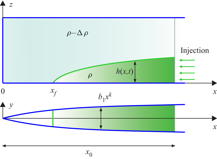
Figure 1. Horizontal channel with varying gap thickness  $b_1x^k$: a converging gravity current in viscous-buoyancy balance propagates toward the origin. Here $x_f$ is the instantaneous front position and $x_0$ is the front position at time $t=0$.
The PL model for a shear-thinning/thickening fluid reads in one dimension
 \begin{equation} \tau = \mu_0|\dot{\gamma}|^{n-1}\dot{\gamma} \end{equation}
in terms of the tangential stress  $\tau$ and of the strain rate $\dot {\gamma }$. The consistency index $\mu _0$ represents a viscosity-like parameter, and the fluid behaviour index $n$ controls the extent of shear-thinning ( $n<1$) or shear-thickening ( $n>1$); $n=1$ corresponds to the Newtonian case. A slightly more complicated description using tensors is required for three-dimensional flows; this general formulation is not reported here as a one-dimensional problem is considered. The fluid advances in a horizontal channel with a gap thickness varying as $b(x)=b_1x^k$ ( $[b_1]=L^{1-k}$, where L is a length scale and $0<k<1$), see figure 1, under the hypotheses of (i) hydrostatic pressure distribution; (ii) $\tau _{xy}\gg \tau _{xz}$ and negligible $\tau _{yz}$, i.e. tangential stress acting on the plane of normal $x$ along the cross direction $y$, is dominant with respect to tangential stress acting on the same plane in vertical direction $z$; (iii) no slip at the side wall at $y=\pm b/2$ and symmetry at $y=0$; (iv) negligible surface tension and no fingering at the interface with the ambient fluid; and (v) inviscid ambient fluid. The lubrication approximation holds and the flow is one-dimensional along the $x$ axis except near the origin, where also the capillary length is comparable to the gap thickness and $\tau _{xz}$ is comparable to $\tau _{xy}$. The streamwise horizontal velocity of the current averaged over the cross-section is
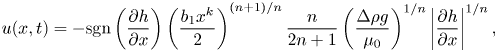 \begin{equation} u(x,t)={-}\mathrm{sgn}\left(\dfrac{\partial h}{\partial x}\right)\left(\dfrac{b_1x^k}{2}\right)^{(n+1)/n}\dfrac{n}{2n+1}\left(\dfrac{\Delta\rho g}{\mu_0}\right)^{1/n} \left|\dfrac{\partial h}{\partial x}\right|^{1/n}, \end{equation}
where  $h(x,t)$ is the current depth, $\Delta \rho \equiv \rho _c-\rho _a$ is the density difference between the intruding current and the ambient fluid and $g$ is gravity. The mass conservation reads
 \begin{equation} \dfrac{\partial h}{\partial t}+\dfrac{1}{x^k}\dfrac{\partial (x^khu)}{\partial x}=0. \end{equation}
 The boundary conditions are motivated by the singular points in the phase plane described later. We anticipate that the boundary conditions allowing a solution are as follows: for  $t<t_c$ are $h=0$ for $x=x_f$ and $u=0$ for $x\to \infty$, where $t_c$ is the touch-down time required by the front of the current to reach the origin of the channel; for $t> t_c$ are $u=0$ and $\partial h/\partial x=0$ for $x=0$; for $t=t_c$ a singularity is reached, which is then removed upon a proper reformulation of the dependent variables. The integral mass conservation, although not specifically involved in the sought self-similar solution of the second kind, are important in numerical integration schemes; the most common representation corresponds to $V\propto t^{\sigma }$, where $\sigma =0$ is the lock release of a finite and constant volume of fluid, $\sigma =1$ is the constant inflow rate, $0<\sigma < 1$ is a waning and $\sigma >1$ is a waxing inflow rate, respectively.
A first-kind self-similar solution cannot be obtained and a second-kind self-similar approach is pursued introducing the phase formalism with the adoption of the independent variables,  $x$ and $t$, as length and time scales, respectively, to render the governing equations dimensionless. We let
 \begin{gather} u(x,t)=\dfrac{x}{t_r}U(x,t_r), \end{gather}
 \begin{gather}h(x,t)=\left(\dfrac{2}{b_1}\right)^{n+1}\left(\dfrac{2n+1}{n}\right)^n\left( \dfrac{\mu_0}{\Delta\rho g}\right)\dfrac{x^{(n+1)(1-k)}}{t_r|t_r|^{n-1}}H(x,t_r), \end{gather}
where  $H$ and $U$ are dimensionless and $t_r=t_c-t$. Here $t_r>0$ represents the pre-closure phase, with the fluid advancing towards the origin of the channel; $t_r<0$ identifies the post-closure phase, with the fluid occupying the entire channel length, the fluid surface undergoing a progressive levelling and the front position being $x_f=0$. In the pre-closure phase $U$ is negative and $H$ is positive, and change sign during the post-closure phase because $t_r$ becomes negative.
Substituting (2.4a) and (2.4b) into (2.2) and (2.3) yields
 \begin{gather} U\left|U\right|^{n-1}+(n+1)(1-k)H+x\dfrac{\partial H}{\partial x}=0, \end{gather}
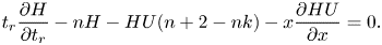 \begin{gather}t_r\dfrac{\partial H}{\partial t_r}-nH-HU(n+2-nk)-x\dfrac{\partial HU}{\partial x}=0. \end{gather}
 We assume a similarity variable  $\xi =xt_r^{-1}|t_r|^{1-\delta }$, where the exponent $\delta$ cannot be determined by using dimensional arguments and must be determined in a different way. Inserting the similarity variable into (2.5a) and (2.5b) gives
 \begin{gather} U\left|U\right|^{n-1}+\xi H'+(n+1)(1-k)H=0, \end{gather}
 \begin{gather}\delta\xi H'+nH+\xi (HU)'+(n+2-nk)HU=0, \end{gather}
where the prime indicates the derivative with respect to  $\xi$ and where the variable $t_r$ does not appear. Eliminating $\xi$ from the two equations results in
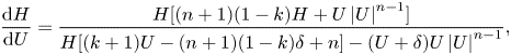 \begin{align} &\dfrac{\mathrm{d}H}{\mathrm{d}U}=\dfrac{H[(n+1)(1-k)H+U\left|U\right|^{n-1}]}{H[(k+1)U-(n+1)(1-k)\delta+n]-(U+\delta)U\left|U\right|^{n-1}}, \end{align}
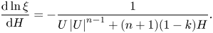 \begin{align} &\dfrac{\mathrm{d}\ln\xi}{\mathrm{d}H}={-}\dfrac{1}{U\left|U\right|^{n-1}+(n+1)(1-k)H}. \end{align}
 These two equations are a set of autonomous planar ODEs, with boundary conditions represented by points in the phase space. We note that the similarity variable has been embedded in its logarithm, with  $\textrm {d}\xi /\xi \equiv \textrm {d}(\ln \xi )$. We define as singular points the simultaneous zeros of numerator and denominator of (2.7a), with a further singular point obtained by setting the denominator to infinity. Hence, there are four singular points, namely
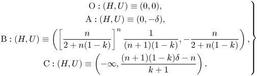 \begin{equation} \left.\begin{gathered} \mathrm{O}:(H,U) \equiv (0,0),\\ \mathrm{A}:(H,U) \equiv(0,-\delta),\\ \mathrm{B}:(H,U) \equiv\left(\left[\dfrac{n}{2+n(1-k)}\right]^n\dfrac{1}{(n+1)(1-k)},-\dfrac{n}{2+n(1-k)}\right),\\ \mathrm{C}:(H,U) \equiv\left(-\infty,\dfrac{(n+1)(1-k)\delta-n}{k+1}\right). \end{gathered}\right\} \end{equation}
In the phase plane a solution connects two points representing the boundary conditions. In this sense, the singular points are crucial because they are the candidates for the role of representatives of the boundary conditions, and the behaviour of the solution must be sought in the neighbourhood of these singularities.
Point O corresponds to null velocity and height at  $t_r=0$ (and to $\xi \to \infty$); point A corresponds to the moving front where $h(x_f(t),t)=0$, with $x_f$ the front position and $x_f(t=0)=x_0$ (and to $\xi =\xi _f$); point B has no specific clear meaning, and from an analytic point of view corresponds to the condition $\textrm {d}^2H/\textrm {d}U^2\equiv \textrm {d}H/\textrm {d}U=0$; point C is active during the post-closure levelling of the current, and represents the asymptotic flow condition (it also corresponds to $\xi =0$). For $n=1$ point B corresponds to the value given in Zheng et al. (Reference Zheng, Christov and Stone2014) (where $n$ in Zheng et al. (Reference Zheng, Christov and Stone2014) corresponds to our $k$).
$k$).
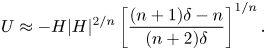
The expansion about point O, computed by assuming  $H=\varpi U^\nu$, substituting in (2.7a) and balancing the smaller-order terms to calculate $\varpi$ and $\nu$, gives
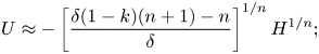 \begin{equation} U\approx{-}\left[\dfrac{\delta(1-k)(n+1)-n}{\delta}\right]^{1/n} H^{1/n}; \end{equation}
the expansion about point A, the front of the current, computed by assuming  $H=\varpi (U+\delta )^\nu$, substituting in (2.7a) and balancing the smaller-order terms, yields
 \begin{equation} U\approx\left[\dfrac{(2+n-kn)\delta-n}{2\delta^n}\right]^{1/n} H-\delta; \end{equation}
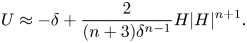
the asymptotic expression for  $H\rightarrow -\infty$ (point C) is computed by assuming $1/H=\varpi (1-U/U_C)^\nu$, substituting in (2.7a) and balancing the smaller-order terms, and gives
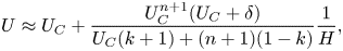 \begin{equation} U\approx U_C+\dfrac{U_C^{n+1}(U_C+\delta)}{U_C(k+1)+(n+1)(1-k)}\dfrac{1}{H}, \end{equation}
where  $U_C$ is the coordinate of the singular point C.
Given these properties of the singular points, we expect that the pre-closure phase is described by an integral curve joining A and O, the post-closure phase by a curve joining O and C.
Numerical integration with Mathematica (Wolfram Research, Inc. 2017) has been performed in the pre-closure time interval ( $t<t_c$) by adopting (2.7a), starting nearby the origin O and assuming that $U=-\epsilon$ with the local expansion for $H$ given by (2.9) in the form
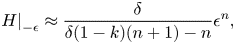 \begin{equation} \left.H\right|_{-\epsilon}\approx\dfrac{\delta}{\delta(1-k)(n+1)-n} \epsilon^n, \end{equation}
with  $\epsilon =10^{-5}$, and computing $H(U)$ in the interval $U \in [-\delta ,-\epsilon ]$. An initial value of $\delta$ was chosen, with iterative modifications of this value and stop criterion when $H(-\delta )<10^{-3}$. The computed eigenvalues, named critical eigenvalues $\delta _c$, are listed in table 2 of Appendix A.
Numerical integration in the post-closure interval ( $t>t_c$) has been performed with the same equation (2.7a) used for the pre-closure interval, but starting near point C where $U=U_C-\epsilon$, with the expansion for $H$ given by (2.11) in the form
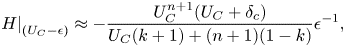 \begin{equation} \left.H\right|_{(U_C-\epsilon)}\approx{-}\dfrac{U_C^{n+1}(U_C+\delta_c)}{U_C(k+1)+(n+1)(1-k)} \epsilon^{{-}1}, \end{equation}
again with  $\epsilon =10^{-5}$, and computing $H(U)$ in the interval $U \in [\epsilon ,U_C-\epsilon ]$. No iteration was required because the value of $\delta _c$ was already known.
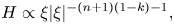
Figure 2 shows the phase portrait of (2.7a) with the trajectories for the critical eigenvalue  $\delta _c=1.5836$ for $n=0.5$ (a typical value for a shear-thinning fluid) and $k=0.5$ (a fracture enlarging with the square root of the abscissa). Continuous and dashed curves describe the pre-closure and post-closure phases, respectively. Figure 3(a) shows the heteroclinic trajectories connecting: (i) point A and point O (continuous curves, pre-closure) and (ii) point O and point C (dashed curves, post-closure or levelling) for fixed $n=0.5$ and increasing $k$ values. For $k\to 1$ the variation of the current depth with $U$ tends to zero near the front and to $-\infty$ near the origin, and $U_C\to 0$. Figure 3(b) shows the same curves but for fixed $k=0.5$ and increasing values of the flow-behaviour index
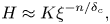
  $n$. Figure 4 shows the eigenvalues as a function of $k$ for different $n$. The asymptotic value for $k\to 1$ is $\delta _c\approx n/[(n+1)(1-k)]$ and corresponds to $U_C\to 0$. The Newtonian fluid ( $n=1$) shows the minimum eigenvalues for a given value of the width coefficient $k$. Relative differences between eigenvalues corresponding to different values of $n$ are modest while $k\leqslant 0.7$, then increase rapidly, especially for very shear-thinning fluids. We observe that the eigenvalues are not monotonic with $n$, and are decreasing with $n$ if $n<1$, increasing if $n>1$, see also the numerical values of $\delta _c$ in table 2. An increase in the eigenvalue results in a higher front velocity ( $U_f=-\delta _c$). This seems to be the result of an interplay between rheology and channel geometry. Observing figure 5(a), it appears that the slope of the free surface current (i.e. the gradient pressure) for $\xi \to \xi _f$ increases with $n$. The front speed results from a balance between gradient pressure and flow resistance. For shear thinning fluids the reduction of resistance with $n$ is more than the reduction of gradient pressure, and the nose of the current is faster for decreasing $n$; for shear-thickening fluids the increase of resistance is less than the increase of the gradient pressure, and again the nose of the current is faster for increasing $n$.
$n$.

Figure 2. Converging gravity current in a fracture of gap thickness  $b=b_1x^k$. Phase portrait of (2.7a) for $n=0.5$ (shear-thinning fluid) and $k=0.5$, with $\delta _c=1.5836$. The singular points are $\mathrm {O}:(0,0)$, $\mathrm {A}:(0,-1.5836)$, $\mathrm {B}:(0.6285, -0.2222)$ and $\mathrm {C}:(-\infty , 0.4585)$. The continuous curve refers to the pre-closure phase, the dashed curve refers to the post-closure (levelling) phase, the thin red vertical line indicates the asymptote in the levelling phase, the dash-dot blue curves are the approximate solutions about points O and A.
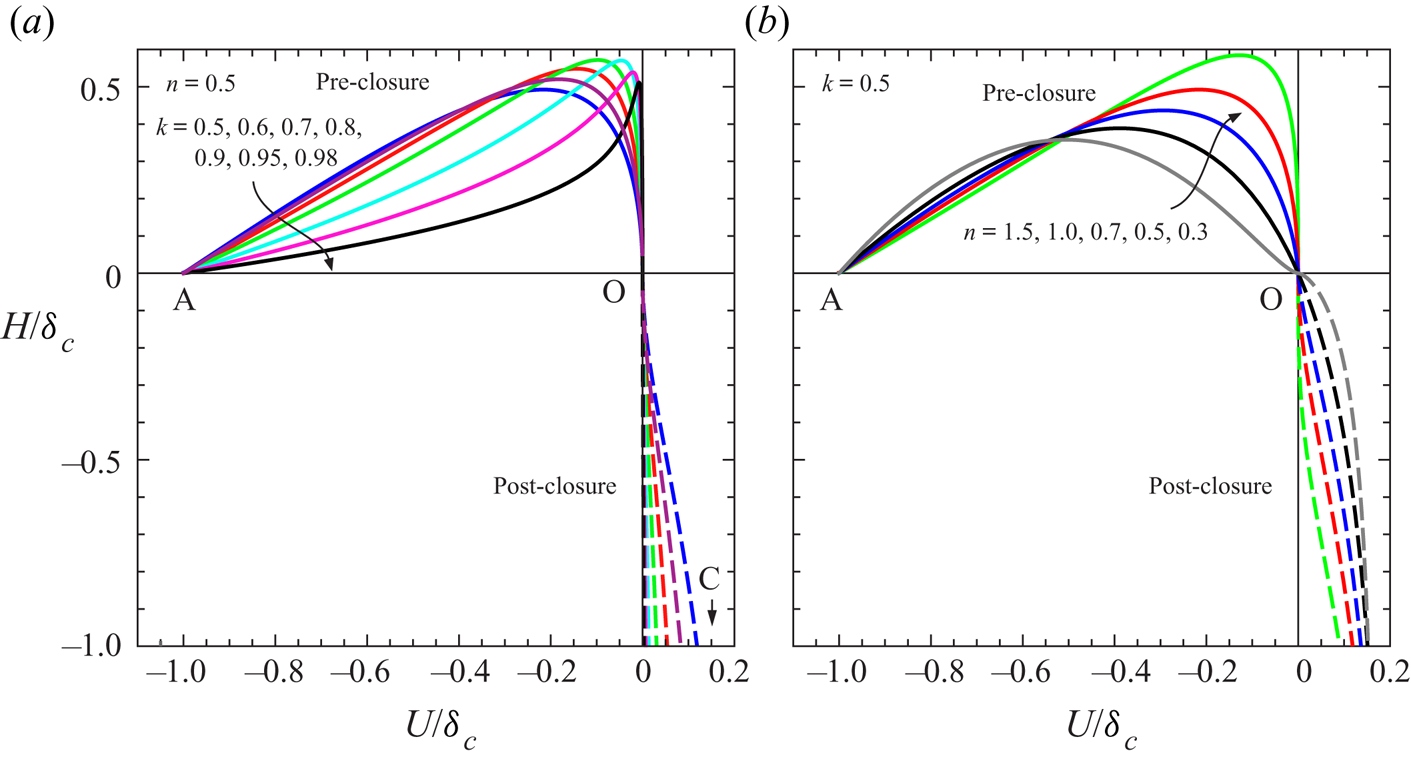
Figure 3. Converging gravity current in a channel of gap thickness  $b=b_1x^k$. Shape of the heteroclinic trajectories in rescaled coordinates for (a) $n=0.5$ (shear-thinning fluid) as $k\rightarrow 1$; (b) $k=0.5$ (a fracture enlarging with the square root of the abscissa) as $n$ varies from 0.5 (shear-thinning) to 1 (Newtonian) and to 1.5 (shear-thickening). Continuous curves refer to pre-closure, dashed curves to post-closure (levelling) phase.
Figure 4. Converging gravity current in a channel of gap thickness  $b=b_1x^k$. Eigenvalues representing the exponent of the similarity variable $\xi =x/(t_c-t)^{\delta _c}$ for fluids with different flow behaviour index $n$. The dashed pink curve refers to a shear-thickening fluid with $n=1.5$, the hatched area is limited by the upper boundary, $1/(1-k)$, and by the lower boundary, $n/[(n+1)(1-k)]$, for $n=0.3$, of the critical eigenvalues.

Figure 5. Converging gravity current in a channel of gap thickness  $b=b_1x^k$. Self-similar current shape profiles and velocity profiles for $k=0.5$ (a fracture enlarging with the square root of the abscissa) and for $n=0.3,0.5,0.7,1.0,1.5$ (a) in the pre-closure phase and (b) in the post-closure phase.
Once the function  $H(U)$ has been computed, in order to evaluate the independent similarity variable $\xi$ it is convenient to rewrite the left-hand side of (2.7b) as $\textrm {d}\ln (\xi )/\textrm {d}U$ via the chain rule and the inverse function theorem using (2.7a), and also to map the domain of varying size $\xi \in [\xi _f,\infty ]$ into $\xi /\xi _f\in [1,\infty ]$. The resulting differential equation
 \begin{equation} \dfrac{\mathrm{d}\ln\xi/\xi_f}{\mathrm{d}U}={-}\dfrac{H}{H[(k+1)U-(n+1)(1-k)\delta_c+n]-(U+\delta_c)U\left|U\right|^{n-1}} \end{equation}
can be integrated in the range  $U \in [-\delta _c,-\epsilon ]$ starting from point A, the front of the current, with the boundary condition $\left .\xi /\xi _f\right |_{U=-\delta _c}=1$, equivalent to $\left .\textrm {d}\ln (\xi /\xi _f)\right |_{U=-\delta _c}=0$. The origin O is reached for $U\to 0$ at $\xi /\xi _f\to \infty$.
Figure 5(a) shows the self-similar current shape profiles and the velocity profiles in the pre-closure phase, for  $k=0.5$ and different values of $n$. We note that velocity profiles are almost coincident, whereas the shape of the current is markedly influenced by the flow behaviour index $n$, with a crest near the front more evident the more shear-thickening is the fluid.
A similar approach is adopted for the post-closure phase, when the front of the current has reached the origin and a progressive levelling occurs. In this phase it is convenient to integrate (2.7b) from point O, with  $\left .\ln \xi \right |_{H=-\epsilon }=-(\delta _c/n)\ln (\epsilon )$. For increasing $H$ (in absolute value), the similarity variable $\xi \to 0$, the neighbourhood of point C where $U\to U_C$. Figure 5(b) shows the current depth and velocity for different values of the fluid behaviour index $n$ and for $k=0.5$. The results for other values of the width exponent $k$ are similar (not shown).
Inserting the expansion (2.9) near the origin O into (2.7b) and solving the resulting differential equation, yields
 \begin{gather} H\approx K\xi^{{-}n/\delta_c}, \end{gather}
 \begin{gather}U\approx{-}\left[\dfrac{\delta_c(1-k)(n+1)-n}{\delta_c}\right]^{1/n} K^{1/n}\xi^{{-}1/\delta_c}. \end{gather}
Switching to dimensional variables gives
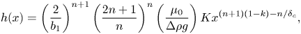 \begin{gather} h(x)=\left(\dfrac{2}{b_1}\right)^{n+1}\left(\dfrac{2n+1}{n}\right)^n\left(\dfrac{\mu_0}{\Delta\rho g}\right)Kx^{(n+1)(1-k)-n/\delta_c}, \end{gather}
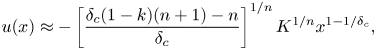 \begin{gather}u(x)\approx{-}\left[\dfrac{\delta_c(1-k)(n+1)-n}{\delta_c}\right]^{1/n} K^{1/n}x^{1-1/\delta_c}, \end{gather}
where  $K$ is a constant. Notably, (2.17) and (2.18) are time independent.
For  $x\to \infty$ the depth of the current grows in the positive direction, hence $\textrm {d} h/\textrm {d} x>0$ that, in turn, implies
 \begin{equation} \delta_c>\dfrac{n}{(n+1)(1-k)}, \end{equation}
which also satisfies the condition of a negative velocity. The minimum value of  $\delta _c$ grows with $n$ and $k$, and tends to infinity for $k\to 1$ (a linearly expanding fracture).
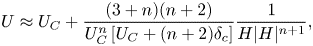
In a similar manner, inserting the expansion (2.11) near point C into (2.7b) and solving the differential equation, yields
 \begin{equation} H\propto \xi|\xi|^{-(n+1)(1-k)-1}, \end{equation}
or
 \begin{equation} h\propto t_r|t_r|^{\delta_c(n+1)(1-k)-n-1}, \end{equation}
in dimensional variables. Equation (2.21) is independent on  $x$ and represents the levelling process near $x=0$.
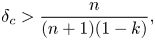
The condition of a time increasing  $h$ during levelling, $\textrm {d}h/\textrm {d}t>0$, equivalent to $\textrm {d}h/\textrm {d}t_r<0$, requires that
 \begin{equation} \dfrac{\textrm{d}h}{\textrm{d}t_r}\propto [\delta_c(n+1)(1-k)-n]t_r|t_r|^{\delta_c(n+1)(1-k)-n-2}<0\rightarrow \delta_c>\dfrac{n}{(n+1)(1-k)}, \end{equation}
coincident with the condition (2.19). Imposing that the levelling process vanishes in time, i.e.
 \begin{equation} \lim_{t_r\to -\infty}\dfrac{\textrm{d}h}{\textrm{d}t_r}=0, \end{equation}
requires that
 \begin{equation} \delta_c<\dfrac{1}{1-k}. \end{equation}
In conclusion, the critical eigenvalue is bounded above and below, i.e.
 \begin{equation} \dfrac{n}{(n+1)(1-k)}<\delta_c<\dfrac{1}{1-k}, \end{equation}
with the two bounds collapsing to  $1/(1-k)=\delta _c$ for an infinitely shear-thickening fluid or $n\to \infty$. Note that the upper bound is independent on the fluid nature. The lower bound for $n=1$ coincides with the result by Zheng et al. (Reference Zheng, Christov and Stone2014) (their $n$ is our $k$). For $k\to 0$ (constant gap thickness) and $n\to \infty$, it results $\delta _c=1$.
Owing to these constraints on the eigenvalues, the time exponent of the depth growth rate at the origin during levelling, defined in (2.21), varies in the range  $[0,1]$, see figure 6 where its value is depicted versus $k$ for different values of the flow behaviour index $n$. As the parameter $k$ describing the growth rate of the fracture gap increases, the same exponent decreases up to a minimum value depending on the fluid rheology, then modestly increases; this is so only for shear-thinning fluids, whereas the exponent for shear-thickening and Newtonian fluids reaches a minimum and remains approximately constant. The minimum value of the exponent in (2.21) is reached for $k=0.75 \text {--}1$. Finally, the exponent increases as the flow behaviour index decreases from shear-thickening to shear-thinning rheology.
Figure 6. Converging gravity current in a channel of gap thickness  $b=b_1x^k$. Time exponent of the growth rate of the depth of the current at the origin during levelling (see (2.21)) as a function of $k$ for fluids with different flow behaviour index $n$ ranging from shear-thinning to shear-thickening. The dashed thin curve indicates the minimum for each $n$ value.
In Appendix B we consider a related problem: the propagation of a plane gravity current of profile  $h(x,t)$ toward the origin of the coordinate system in an heterogeneous porous medium with spatially variable permeability and porosity. If both quantities exhibit a PL variation in the streamwise direction $x$, a formal analogy can be established between two domains, the porous medium and the Hele-Shaw cell or channel of variable gap thickness. The analogy is subject to constraints in the values of parameters describing the heterogeneity as detailed in Appendix B.
3. Converging axisymmetric flow
We consider the converging flow of a cylindrical gravity current as shown in figure 7: the current propagates towards the origin of a cylindrical coordinate system. We assume again: (i) the current to be thin, allowing a hydrostatic pressure distribution; (ii)  $\tau _{rz}$ to be the dominant shear, with negligible contributions by $\tau _{r\theta }$ and $\tau _{\theta z}$; and (iii) no surface tension effects and no fingering at the interface with the ambient fluid; (iv) inviscid ambient fluid. Gravity is the driving force balanced by viscous forces. In the limits of lubrication model, the vertically averaged horizontal velocity in the radial direction, calculated by imposing the no slip condition $u=0$ for $z=0$ and a zero tangential stress at the interface with the ambient fluid, corresponding to $\partial u/\partial x=0$ for $z=h$, is
 \begin{equation} u(r,t)={-}\textrm{sgn}\left(\dfrac{\partial h}{\partial r}\right)h^{(n+1)/n}\dfrac{n}{2n+1}\left(\dfrac{\Delta\rho g}{\mu_0}\right)^{1/n}\left|\dfrac{\partial h}{\partial r}\right|^{1/n}, \end{equation}
and mass conservation reads
 \begin{equation} \dfrac{\partial h}{\partial t}+\dfrac{1}{r}\dfrac{\partial (ruh)}{\partial r}=0. \end{equation}
Again, in a general approach we should specify the initial and boundary conditions, but as already discussed in § 2, the boundary conditions are motivated by the singular points in the phase plane.
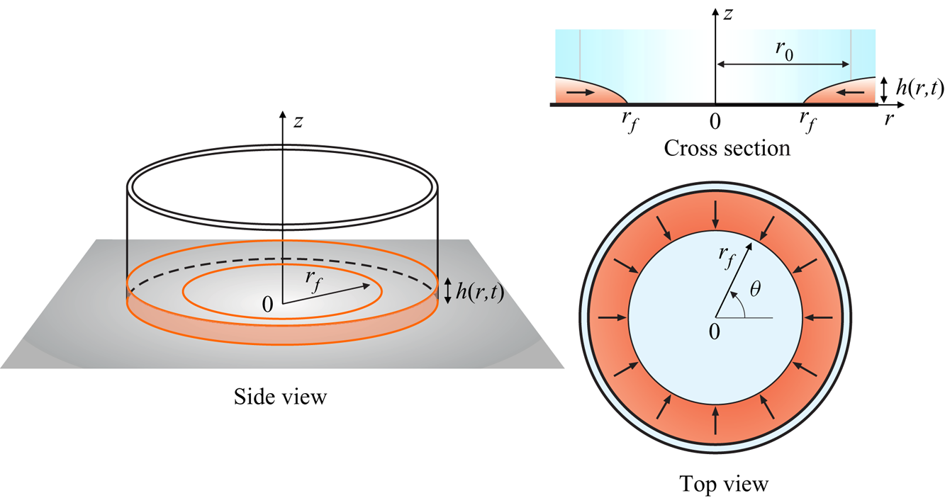
Figure 7. Radial converging flow: a gravity current in viscous-buoyancy balance propagates towards the origin. Here  $r_f$ is the instantaneous front position and $r_0$ is the front position at time $t=0$.
The dependent variables  $u$ and $h$ are rendered non-dimensional as follows:
 \begin{gather} u(r,t)=\dfrac{r}{t_r}U(r,t_r), \end{gather}
 \begin{gather}h(r,t)=\left(\dfrac{2n+1}{n}\right)^{n/(n+2)}\left(\dfrac{\mu_0}{\Delta\rho g}\right)^{1/(n+2)} \dfrac{r^{(n+1)/(n+2)}}{t_r|t_r|^{{-}2/(n+2)}}H(r,t_r). \end{gather}
Then the similarity independent variable  $\xi =r t_r^{-1}|t_r|^{1-\delta }$ is introduced, where $\delta$ is the yet unknown eigenvalue. With the same approach described for converging flow in a horizontal fracture, equations (3.1) and (3.2) are rearranged to obtain
 \begin{align} &\dfrac{\mathrm{d}U}{\mathrm{d}H}=\dfrac{H|H|^{n+1}[2(n+2)U-(n+1)\delta+n]-(U+\delta)(n+2)U\left|U\right|^{n-1}}{H[(n+1)H|H|^{n+1}+(n+2)U\left|U\right|^{n-1}]}, \end{align}
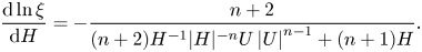 \begin{align} &\dfrac{\mathrm{d}\ln\xi}{\mathrm{d}H}={-}\dfrac{n+2}{(n+2)H^{{-}1}|H|^{{-}n}U\left|U\right|^{n-1}+(n+1)H}. \end{align}
The singular points are
 \begin{equation} \left.\begin{gathered} \mathrm{O}:(H,U) \equiv (0,0),\\ \mathrm{A}:(H,U) \equiv(0,-\delta),\\ \mathrm{B}:(H,U) \equiv\left(\left[\dfrac{n+2}{n+1}\right]^{1/(n+2)}\left[\dfrac{n}{5+3n}\right]^{n/(n+2)},-\dfrac{n}{5+3n}\right),\\ \mathrm{C}:(H,U) \equiv\left(-\infty,\dfrac{(n+1)\delta-n}{2(n+2)}\right), \end{gathered}\right\} \end{equation}
and have the same meaning of the points described for converging fracture flow.
The case  $n=1$ refers to a Newtonian fluid, and (3.4a)–(3.4b) become
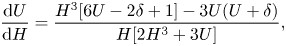 \begin{align} &\dfrac{\mathrm{d}U}{\mathrm{d}H}=\dfrac{H^{3}[6U-2\delta+1]-3U(U+\delta)}{H[2H^{3}+3U]}, \end{align}
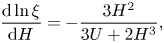 \begin{align} &\dfrac{\mathrm{d}\ln\xi}{\mathrm{d}H}={-}\dfrac{3H^2}{3U+2H^3}, \end{align}
and the singular points are
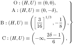 \begin{equation} \left.\begin{gathered} \mathrm{O}:(H,U) \equiv (0,0),\\ \mathrm{A}:(H,U) \equiv(0,-\delta),\\ \mathrm{B}:(H,U) \equiv\left(\left[\dfrac{3}{16}\right]^{1/3},-\dfrac{1}{8}\right),\\ \mathrm{C}:(H,U) \equiv\left(-\infty,\dfrac{2\delta-1}{6}\right), \end{gathered}\right\} \end{equation}
corresponding to the differential problem in Diez et al. (Reference Diez, Gratton and Gratton1992b) with a different definition of the variables. The results are equivalent to those reported in McCue et al. (Reference McCue, Jin, Moroney, Lo, Chou and Simpson2019), where a slightly different approach and a broader perspective is adopted, with an improved clarity of the various steps. See also Gratton & Perazzo (Reference Gratton and Perazzo2010).
Numerical integration of the pre-closure phase starts with a first tentative value of  $\delta$ and moving from the origin O ( $\xi \to \infty$), where $H\to 0$ and the solution for $U$ is approximated by
 \begin{equation} U\approx{-}H|H|^{2/n}\left[\dfrac{(n+1)\delta-n}{(n+2)\delta}\right]^{1/n}. \end{equation}
Upon successive iterations with changes of the  $\delta$ value, the integral curve reaches exactly point A ( $\xi =\xi _f$), the front of the gravity current, where $H\to 0$ and the approximate solution for $U$ is
 \begin{equation} U\approx{-}\delta+\dfrac{2}{(n+3)\delta^{n-1}}H|H|^{n+1}. \end{equation}
The value of  $\delta$ that allows the integral curve to reach point A from O is the critical eigenvalue $\delta _c$.
Numerical integration of the post-closure phase starts about point C, where  $H\to -\infty$ (and $\xi \to 0$) and where the approximate solution for $U$ is
 \begin{equation} U\approx U_C+\dfrac{(3+n)(n+2)}{U_C^n\left[U_C+(n+2)\delta_c\right]}\dfrac{1}{H|H|^{n+1}}, \end{equation}
and the integral curve reaches point O ( $\xi \to \infty$), where the approximate solution is (3.8). In this second integration, iterations are not necessary because $\delta _c$ is already known. The expansion about the singular points O, A and C has been obtained in the same way as that reported for the differential problem describing the gravity current in a converging channels, see § 2.
Figure 8 shows the phase portrait for a shear-thinning fluid with  $n=0.5$, with the integral curves for the pre- and post-closure phases, corresponding to an eigenvalue $\delta _c=0.78261$. The eigenvalues for different values of $n$ are listed in table 3 of Appendix A and are shown in figure 9, where a shear-thinning behaviour is accompanied by higher $\delta _c$, although the variability is quite modest; the corresponding integral curves are depicted in figure 10(a), followed by the shape profiles and velocity profiles in the pre-closure phase in figure 10(b). No specific trend is observed, although the thickness of the current immediately behind the front is larger for more shear-thinning fluids. The horizontal velocity is almost indistinguishable for currents with different value of the fluid behaviour index. The results for the eigenvalues coincide with those shown in Figure 1 in Gratton & Perazzo (Reference Gratton and Perazzo2010), after converting the horizontal axis and with their $\lambda$ equal to $1/n$ in the present notation.
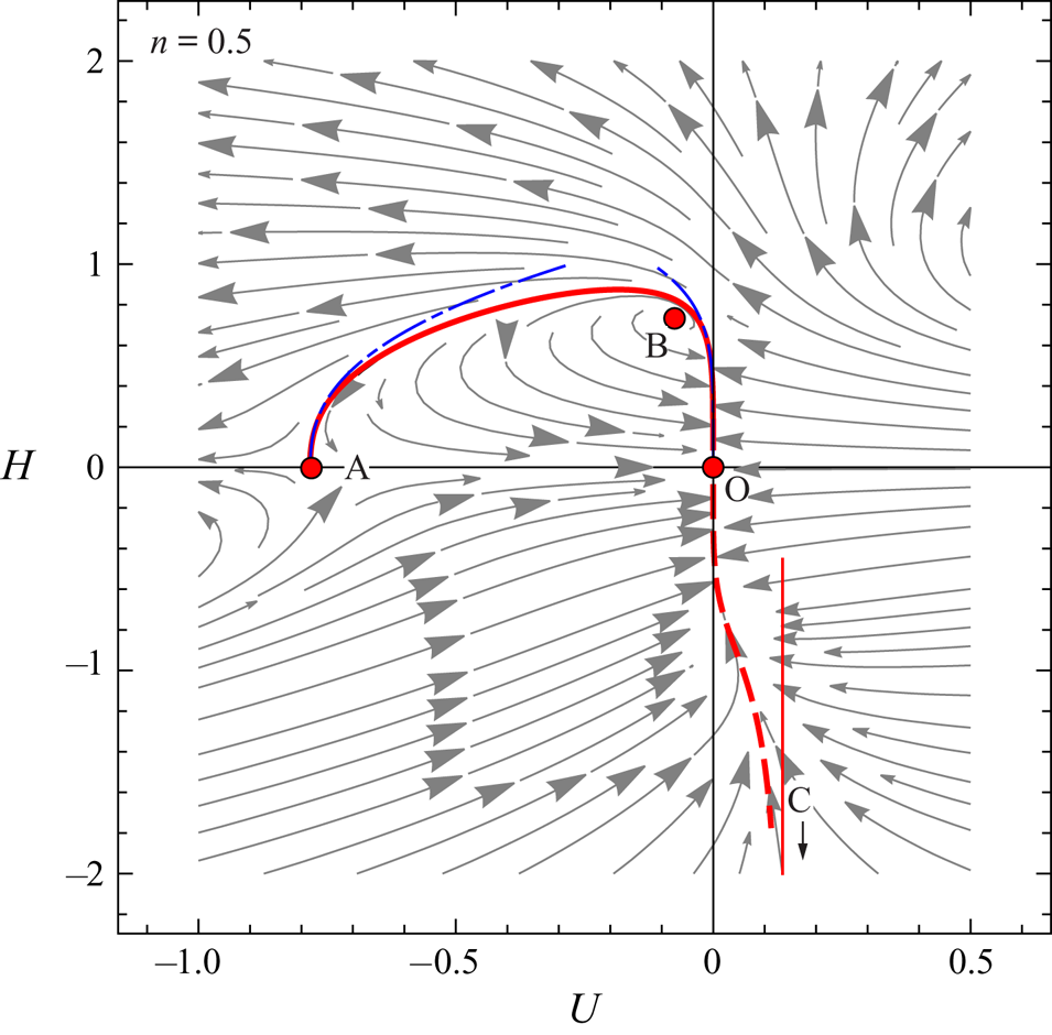
Figure 8. Converging radial gravity current. Phase portrait of (3.4a) for  $n=0.5$ (shear-thinning fluid), $\delta _c=0.78261$. The continuous curve refers to the pre-closure phase, the dashed curve refers to the post-closure (levelling) phase, the thin red vertical line indicates the asymptote in the levelling phase and the dash-dot blue curves are the approximate solutions about points O and A.
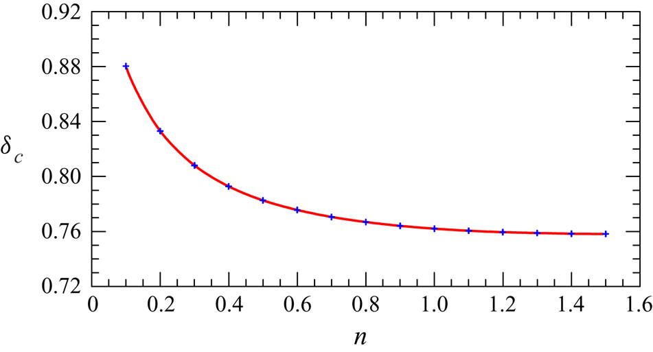
Figure 9. Converging radial gravity current. Eigenvalues representing the exponent of the similarity variable  $\xi =x/(t_c-t)^{\delta }$ for axisymmetric flow towards the origin for fluids with different flow behaviour index $n$.
$n$.

Figure 10. Converging radial gravity current: (a) shape of the heteroclinic trajectories in the pre-closure (continuous curves) and post-closure (dashed curves) phase; and (b) shape profiles and velocity profiles in the pre-closure phase as  $n$ varies from 0.5 (shear-thinning) to 1 (Newtonian) and to 1.5 (shear-thickening).
The behaviour of the integral curves approaching O can be obtained by expanding  $H=a_0\xi ^b+a_1\xi ^{b+1}+\ldots\, $. Then introducing the approximation (3.8) in (3.4b) and balancing yields
 \begin{gather} H=K\xi^{{-}n/[\delta_c(n+2)]}, \end{gather}
 \begin{gather}U={-}K^{(2+n)/n}\left[\dfrac{(n+1)\delta_c-n}{(n+2)\delta_c}\right]^{1/n}\xi^{{-}1/\delta_c}, \end{gather}
where  $K$ is a constant. Switching to dimensional variables, one obtains for the current depth and velocity
 \begin{gather} h(r)=\left(\dfrac{2n+1}{n}\right)^{{n}/({n+2})}\left(\dfrac{\mu_0}{\delta_c\rho g}\right)^{{1}/({n+2})} Kr^{({(n+1)\delta_c-n})/({(n+2)\delta_c})}, \end{gather}
 \begin{gather}u(r)={-}K^{(2+n)/n}\left[\dfrac{(n+1)\delta_c-n}{(n+2)\delta_c}\right]^{1/n}r^{(\delta_c-1)/\delta_c}, \end{gather}
that are time-independent. For  $r\to \infty$, the depth of the current grows in the positive direction, hence $\textrm {d} h/\textrm {d} r>0$ that in turn implies $\delta _c>n/(n+1)$, which also ensures a negative velocity.
A similar analysis can be conducted to describe the post-closure phase, with results similar to those obtained for converging flow in a horizontal fracture.
4. Experimental validation
4.1. Experimental set-up
Three different experimental set-ups were developed in the Laboratory of Hydraulics of the University of Parma in order to validate the theoretical models.
The first set-up consists of a tank to reproduce the propagation of gravity currents in converging channel flow. The channel consists of two rectangular plates, 150 cm long and 20 cm high, with a front wall made of transparent plastic for an easy visualization, while the back wall is made of yellow polyvinyl chloride (PVC) machined with a computerized numerical control machine; the gap thickness is  $b(x)=b_1\,x^{0.6}$, where $x$ is the abscissa with origin at the corner, as shown in figure 11; $b_1=0.01176\ \textrm {m}^{0.4}$ and the width of the channel at $x=150\ \textrm {cm}$ equals $1.5\ \textrm {cm}$. Lock release gravity currents were generated with different lengths of the lock, equal to $12, 14, 20, 30 \ \mathrm {cm}$. One experiment was performed with a different boundary condition of given flux, in order to check the sensitivity of the solution to the inflow mode. A similar set-up was adopted in Zheng et al. (Reference Zheng, Christov and Stone2014) and also documented in Ghodgaonkar (Reference Ghodgaonkar2019), with a length of $75\ \textrm {cm}$. With this set-up, the heavy fluid was Newtonian or non-Newtonian PL shear-thinning, whereas the ambient fluid was always air.
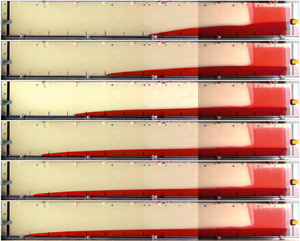
Figure 11. Experimental set-up  $\#1$, a tank with a gap thickness of $b_1 \, x^{0.6}$: (a) front view; (b) top view; (c) a photo during one of the tests; the lock is almost empty but a thin layer of fluid still adheres to the transparent wall, marking the volume occupied by the fluid in the lock before lifting the gate.
A second series of experiments reproduced radial converging gravity currents and was carried out in a transparent plastic cell shaped as a circular sector (a wedge) with an angle at the centre  $\beta = 12^\circ$, a radius $R=75\ \textrm {cm}$ and a height of $h=18\ \textrm {cm}$. The front, side and top view are shown in figure 12(a–c), respectively. The front vertical wall is rigidly attached to the bottom, while the back wall is removable. At a distance $r_0=60\ \textrm {cm}$ a vertical gate is inserted in order to separate the heavy fluid in the upstream lock from the light ambient fluid in the downstream chamber. Three clamps are applied on top of the tank in order to push the walls against the bottom and prevent any leakage. Figure 12(d) is a photograph of the experimental apparatus.
Figure 12. Experimental set-up  $\#2$, a circular sector cell with an angle at the centre $\beta = 12^\circ$: (a) front view; (b) lateral view; (c) top view; and (d) snapshot of the tank.
A third set of experiments for radial converging gravity currents was conducted in a fully metallic cylinder with an inner radius of  $R_2 = 30 \ \mathrm {cm}$ (figure 13). A smaller cylinder with an external radius $R_1 = 19.5 \ \mathrm {cm}$ is positioned concentrically to the prior one and pushed against the glass bottom (a soft rubber sealing gasket is present) in order to create an annular lock with a gap $\Delta R = R_2 - R_1 = 10.5 \ \mathrm {cm}$. Particular attention was paid to the levelling of the base of the apparatus, so as to prevent asymmetries due to the gravitational force. An electronic level is used for this purpose, with an accuracy of $0.1^{\circ }$. The annulus is filled with dense fluid up to a depth of $h_0 = 3.3 \text {--} 4.5 \ \mathrm {cm}$. The inner cylinder is filled with light ambient fluid. At the beginning of the experiments, the inner cylinder is lifted up to a known height $h < h_0$. A similar set-up was used in Diez et al. (Reference Diez, Gratton and Gratton1992b), with radius of the external/internal cylinder of 20 and 5 cm, respectively.
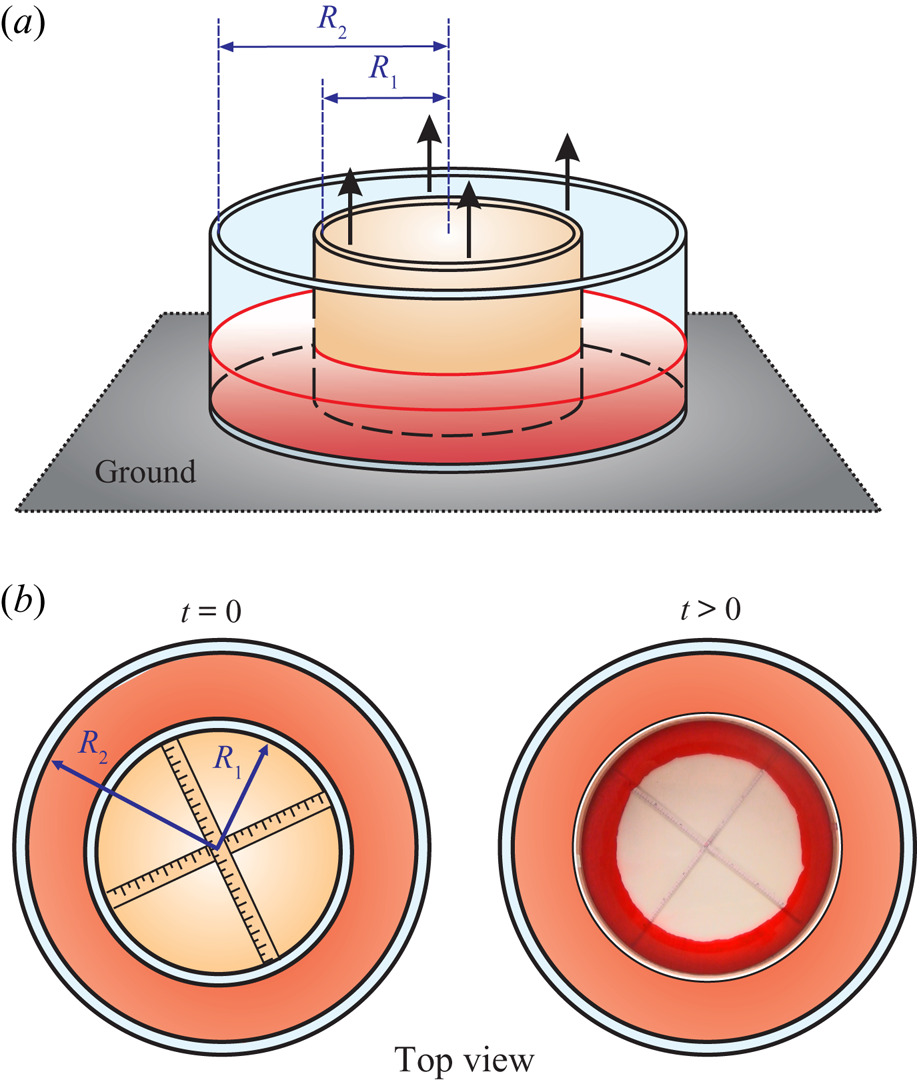
Figure 13. Experimental set-up  $\#3$, a radial symmetric cell: (a) front view; (b) top view at $t = 0$, before the lift of the inner cylinder (sketch), and for $t>0$, after the lift of the inner cylinder (photo).
For the currents in converging channel flow (set-up  $\#1$), the Newtonian fluids were prepared with glycerol, while the non-Newtonian fluids were prepared with (i) a mixture of water (95 % vol.), glycerol (5 % vol.) and carboxymethyl cellulose (CMC, 2 % by weight), or a (ii) a mixture of water (40 % vol.), glycerol (60 % vol.) and E415 (0.1 % by weight). All the non-Newtonian fluids have PL shear-thinning rheology.
For the radial converging currents (set-ups #2 and #3), the Newtonian fluids were prepared with either glycerol or a mixture of glycerol, salt and water, and non-Newtonian fluids with a mixture of water (60 % vol.), glycerol (40 % vol.) and xanthan gum (E415, 0.25 % by weight). The light ambient fluid is water or a mixture of water, salt and glycerol with a density slightly less than the current fluid. The combination of different ambient fluids and intruding fluids was required in order to guarantee the viscous regime, with negligible inertial effects, and to increase the duration of the experiments for an accurate estimation of  $t_c$. Aniline water color was finally added to the denser fluid for an easy visualization of the propagating current.
The rheology was measured by the parallel plate twin-driver MCR702 rheometer by Anton Paar, at a temperature of  $\varTheta = 25\text {--}27^{\circ }$, equal to the ambient temperature during the experiments. Several different tests were performed in order to evaluate the fluid behaviour index and consistency index for non-Newtonian fluids, and the dynamic viscosity of Newtonian fluids. Figure 14 shows the experimental shear-stress/shear-rate curves for two different shear-thinning fluids. The limited range of shear rate is dictated by the evidence that, except at the early stage of the current propagation, after the gate lift, the average shear rate is quite modest. The estimated accuracy is $\Delta n/n\leqslant 4\,\%$ and $\Delta \mu _0/\mu _0\le 6\,\%$. The mass density of the fluids was measured by a hydrometer (STV350023 Salmoraghi), and by the DMA 5000 by Anton Paar, with an accuracy of $\Delta \rho /\rho _0 \leqslant 0.1\,\%$.
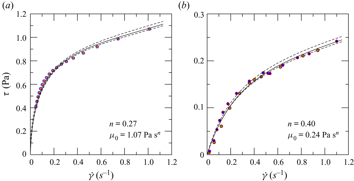
Figure 14. Experimental rheometry of two shear-thinning fluids: (a) mixture of water, NaCl and xanthan gum,  $\varTheta =27\,^{\circ }\textrm {C}$; (b) mixture of water, NaCl and xanthan gum, with two series of measurements to check repeatability, $\varTheta =25\,^{\circ }\textrm {C}$. The solid curves are the PL interpolation and the dashed curves are the 95 % confidence limits.
The profiles of the advancing current after the lift of the gate, are recorded by either a high-resolution video camera (Canon Legria  $1920 \times 1080$ pixels) operating at 25 frames per second (fps), or an iPhone 4k video camera working at 30 fps. For some experiments both videos were used in order to capture the whole profile of the current with an adequate resolution, see figure 11(c) where the panoramic image results from two frames extracted from two synoptic videos. The frames extracted from the video are post-processed using a Matlab code that converts pixels into metric coordinates. This conversion is possible thanks to a square grid attached onto the inner side of the front vertical wall, which allows compensation of the optical distortion. The overall accuracy in detecting the position of the nose and the profile of the current is approximately 0.1 cm, while the accuracy in measuring time is negligible (1/50–1/60 s).
Figure 15 shows a sequence of snapshots for one of the experiments in lock-release, experiment 11, with both pre- and post-closure instants. After closure, the effect of capillarity near the origin is evident, with an increase in the level compared with the average value observed far from the origin. Local level for post-closure analysis was obtained correcting data for capillarity uprise.
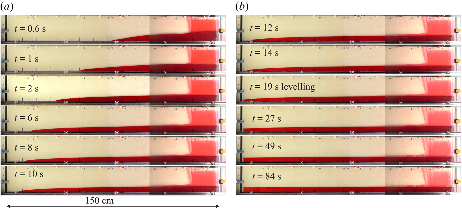
Figure 15. Time lapse of the current profile for experiment 11 in a channel of varying gap thickness. Closure is at  $t_c=16.4\ \textrm {s}$, then levelling starts.
4.2. Experiments
The parameters of the experiments are listed in table 1; 10 experiments were performed in the converging channel and 11 experiments in radial geometry, either in the  $12^\circ$ sector or in the full circle configuration. The theory assumes the dominance of viscous and buoyancy forces over inertia. The Reynolds number for channel flow can be expressed as ratio between the inertial and viscous forces per unit volume,
 \begin{equation} F_i\sim \Delta\rho\dfrac{u^2}{L},\quad F_v\sim\mu_0\dfrac{u^n}{L^{n+1}},\quad \rightarrow {Re}=\dfrac{\Delta\rho u^{2-n}L^n}{\mu_0}, \end{equation}
where  $L$ is taken to be equal to the channel maximum width $L=b_1x_0^k$. The velocity scale can be assumed equal to $x_0/t_c$, hence
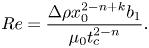 \begin{equation} {Re}= \dfrac{\Delta\rho x_0^{2-n+k}b_1}{\mu_0t_c^{2-n}}. \end{equation}
Table 1. Parameters for the experiments on converging flow in a channel of variable thickness and in radial geometry. The second column indicates the geometry of the flow field, where ‘c’ denotes channel and ‘r12’ and ‘r360’ denote radial geometry with an angle at the centre of  $12^\circ$ and $360^\circ$, respectively. We use ‘c-Q’, ‘l-r’ and ‘c-h’ to denote constant inflow rate, lock-release and constant head; $h$ and $h_0$ are the constant head or the initial depth in the lock; $a$ is the height of the slot at the bottom of the gate; $r_0,x_0$ is the initial position of the front of the current in radial geometry and in the channel; $n$ and $\mu _0$ are the fluid behaviour index and the consistency index (the viscosity for Newtonian fluids) of the current fluid, respectively; $\rho _c,\rho _a$ are the current/ambient fluid density; $t_c$ is the touch-down time; and Re is the Reynolds number according to the expressions (4.2)–(4.4), where an average value $h=2\ \textrm {cm}$ is assumed for radial gravity currents.
For radial gravity currents a similar analysis brings to a Reynolds number defined as
 \begin{equation} {Re}=\dfrac{\Delta\rho u^{2-n}h^{n+1}}{\mu_oR},\quad\textrm{with}\ u\sim\left(\dfrac{\Delta\rho g}{\mu_0}\right)^{1/n}\dfrac{h^{(n+2)/n}}{R^{1/n}}, \end{equation}
hence
 \begin{equation} {Re}=\left(\dfrac{\Delta\rho}{\mu_0}\right)^{2/n}g^{(2-n)/n}\dfrac{h^{(n+4)/n}}{R^{2/n}}. \end{equation}
 The values of Reynolds number listed in the last column of table 1 refer to the initial stage of the current propagation; for channel flow  ${Re}<1$ and for radial flow ${Re} \ll 1$, with only one test initially characterized by ${Re}\approx 0.8$. In the other tests, inertial effects are negligible from the very beginning, and the viscous balance dominates the advancement of the currents at all stages.
Figure 16 shows the time series of the front position for the experiments in converging channel flow. The experiments are separated in two groups, namely Newtonian and shear-thinning gravity currents. For the former tests the theoretical eigenvalue is  $\delta _c=1.787$ and the corresponding trajectory is fairly well followed by the experiments. Similar experiments were conducted in Zheng et al. (Reference Zheng, Christov and Stone2014) in channels with different width exponent $k$, although only in lock-release mode. In the present Newtonian subset, four tests are in lock-release mode, whereas experiment 1 is a constant influx experiment. The results indicate that in lock-release mode the current requires a much longer time to forget the initial condition and to reach self-similarity, whereas with a constant influx the current evolves rather quickly to reach the intermediate asymptotic regime of self-similarity. The different lengths of the locks do not have a significant effect on the current propagation in the far field. The grey symbols are considered outliers attributed to several disturbances and interferences, such as capillarity and three dimensionality of the flow field not modelled in the theory. Experiments 3 and 5 are a repetition with the same fluid and under the same conditions, to obtain an estimate of the repeatability and uncertainty.
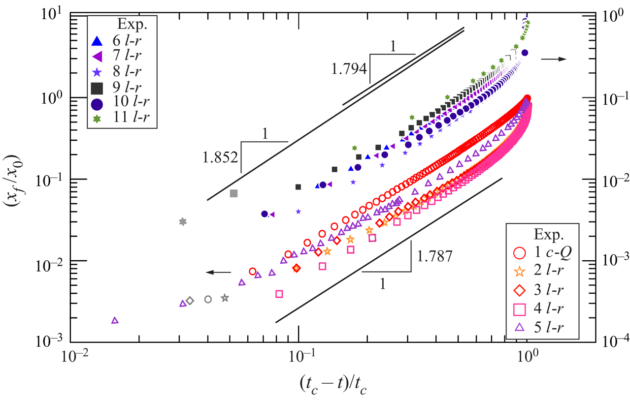
Figure 16. Front position of gravity currents in converging channel flow with  $k=0.6$. Experiments 1–5 refer to Newtonian fluid (left vertical axis) and experiments 6–11 refer to shear-thinning fluids (right vertical axis). The straight lines correspond to the theoretical curves for $n=1$ and $n=0.54\text {--}0.90$, respectively, with eigenvalues $\delta _c=1.787$ and $\delta _c=1.852\text {--}1.794$. The parameters of the experiments are listed in table 1.
For the non-Newtonian fluid experiments the fluid behaviour index ranges from 0.54 to 0.90, and the consistency index ranges from 0.42 to  $2.63\ \textrm {Pa}\ \textrm {s}^n$. The two straight lines in figure 16 correspond to extreme values of $\delta _c\approx 1.79$ and $\approx 1.85$. Again the experimental results, all in lock-release mode, adequately follow the theory, reaching the self-similar regime although the differences with the value of $n$ cannot be appreciated. Essentially, the long tank favours the evolution of the current with enough space to forget the inlet and initial conditions and before reaching the proximity of the origin, where capillarity renders the theoretical model invalid.
A comparison of the shape of the current with the experiments is reported for two experiments, with Newtonian and PL fluids, respectively. A main variable in checking the validity of the model is the time position of the front of the current. We expect that  $x_f(t)\propto t_r^{\delta _c}$, hence
 \begin{equation} \dfrac{x_f(t)}{x_0}=\alpha\left(\dfrac{t_r}{t_c}\right)^{\delta_c}, \end{equation}
where the dimensionless coefficient  $\alpha$ is the intercept of the straight interpolating line in a diagram $x_f/x_0-t_r/t_c$ drawn in logarithmic scale. We also have the result
 \begin{equation} \xi_f=\dfrac{\alpha x_0}{t_c^{\delta_c}}, \end{equation}
which is a constant for each experiment. The value of  $\alpha$ is obtained by interpolating the experimental front position of the advancing current in pre-closure phase.
Figure 17(a,b) refers to the pre-closure phase for experiments 5 and 11, with experimental profiles sampled in several sections at different times and the continuous curve representing the theoretical model. For the Newtonian fluid case, the early time profiles show a significant discrepancy with theory, which however decreases after approximately  $190\ \textrm {s}$. That means that at least for approximately $35\ \textrm {s}$ the current is in self-similar regime, ended by the insurgence of capillarity effects near the origin. For the PL fluid, experiment 11, the profile at $t=6\ \textrm {s}$ differs from the rest of the time snapshots which collapse onto one curve, so they are self-similar; all profiles differ from theory at the peak around $\xi /\xi _f\approx 2.5$ and are in excess to the same degree that the profile at $t=6\ \textrm {s}$ differs around $\xi /\xi _f\approx 10$, and is in defect. We observe that experiment 11 has the highest initial Reynolds number and shows an initial stage when inertial effects are comparable to viscous effects. However, the current forgets its original regime and evolves towards self-similarity. This is another validation of the memoryless behaviour of the gravity currents, which not only forget the type of influx (lock-release or constant influx), but also their initial regime (inertial or in transition). The analysis of the time requested by self-similar solutions to approximate within a given accuracy the (numerical) solutions was discussed by Ball et al. (Reference Ball, Huppert, Lister and Neufeld2017) and Ball & Huppert (Reference Ball and Huppert2019) in the context of gravity currents, also considering different shapes of the lock or inflow rate variations. The results obtained for first-kind self-similar solutions can be extended to experiments and to second-kind self-similar processes: the approximation improves with time, unless disturbances effects (such as capillarity) render the model invalid. It explains the different agreement in times between experiments and theory, which improves for $t>6\ \textrm {s}$ although the peak value of $H$ is underestimated by approximately $15\,\%$. The numerous approximations of the model are responsible for this discrepancy, but the self-similar nature of the profiles is adequately confirmed.
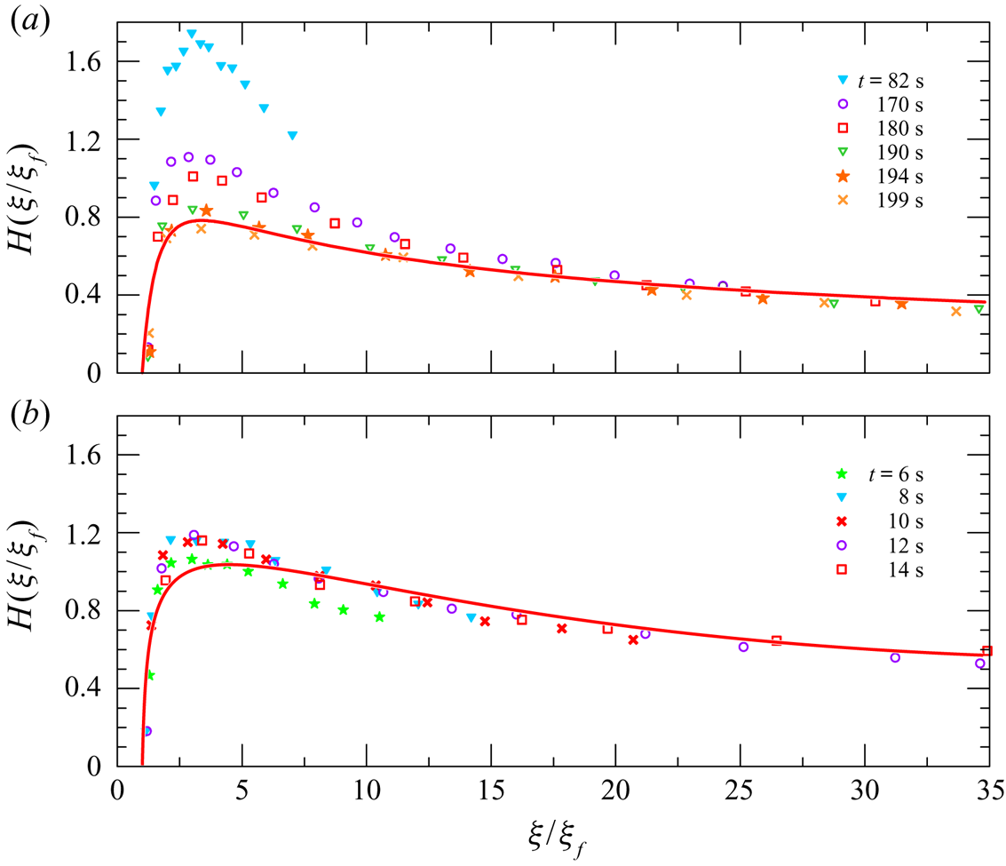
Figure 17. Experimental profiles of the current in converging channel flow with  $k=0.6$ during pre-closure (symbols) compared with the theoretical self-similar solution (bold line): (a) experiment 5, Newtonian fluid, $t_c=229\ \textrm {s}$, $\delta _c=1.7874$, $\alpha =0.30$; (b) experiment 11, PL fluid, $t_c=16.4\ \textrm {s}$, $\delta _c=1.8534$, $\alpha =0.19$.
A comparison between experiments and theory has been conducted also for the post-closure stage, with the current levelling near the origin. In this case the pre-factor refers to the time evolution of the current depth in the origin, where, in the self-similar stage, we have the result
 \begin{equation} \dfrac{h(0,t)}{h_\infty}=\alpha'\left(\dfrac{-t_r}{t_c}\right)^{\delta_c(n+1)(1-k)-n}. \end{equation}
 Figure 18 shows the comparison between theory and experiments for experiments 5 and 11. During post-closure, the pre-factor  $\alpha '$ is computed by considering the experimental time evolution of the depth $h(0,t)$, which is initially varying according to (4.7), see the insets. The theoretical exponent of the current depth growth in the origin is $\delta _c(n+1)(1-k)-n$, equal to 0.429 and to 0.602 for experiments 5 and 11, respectively; the experimental values are 0.42 and 0.51, with a fairly good agreement for the first, an acceptable agreement for the second. The overall adherence between experiments and theory is striking, with a better collapse of the experimental data and of the theoretical curve for increasing time after closure.
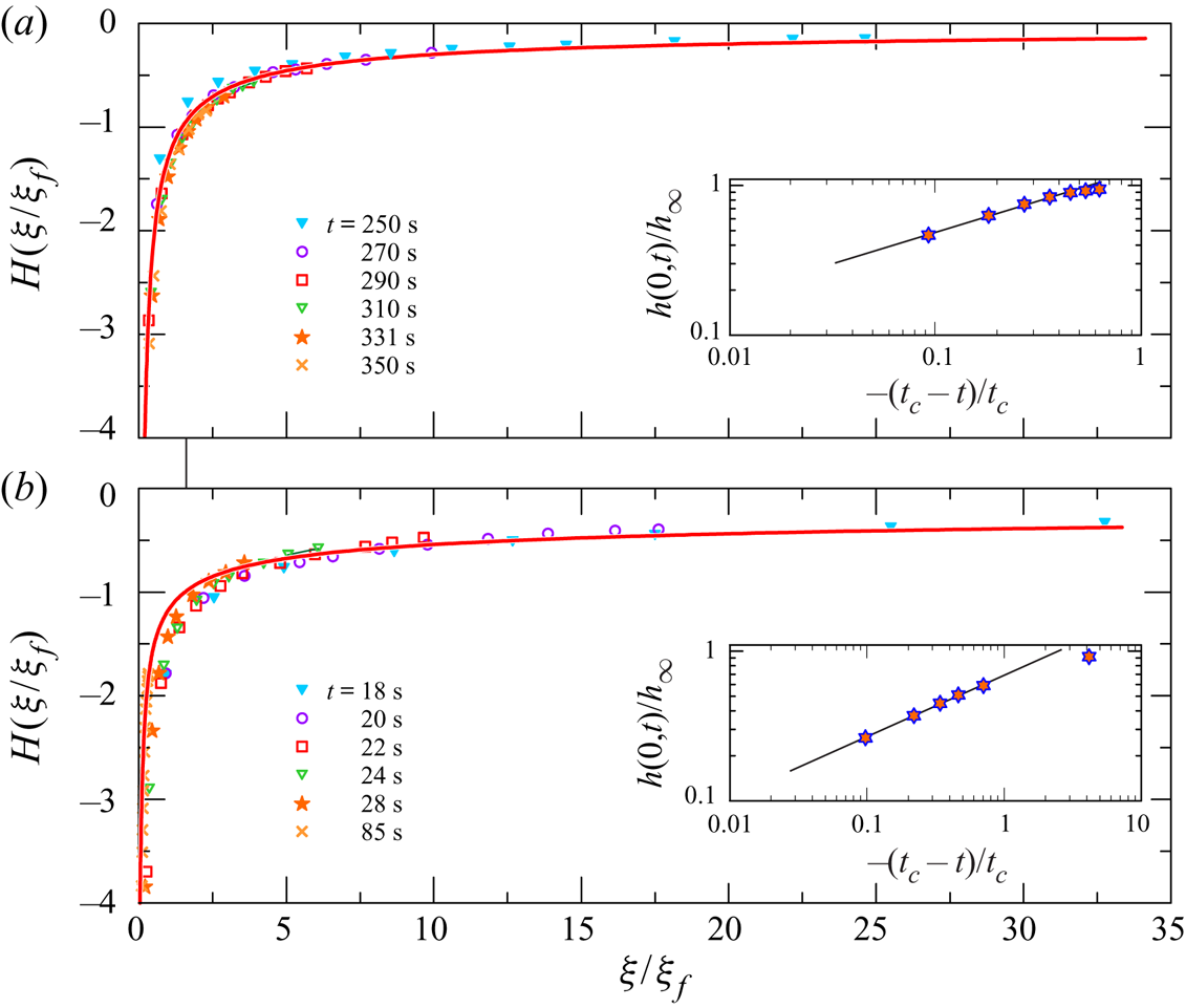
Figure 18. Experimental profiles of the current in converging channel flow with  $k=0.6$ during levelling (symbols) compared with the theoretical self-similar solution (bold line): (a) experiment 5, Newtonian fluid $n=1$, $t_c=229\ \textrm {s}$, $\delta _c=1.7874$, $\alpha '=1.29$; (b) experiment 11, PL fluid $n=0.54$, $t_c=16.4\ \textrm {s}$, $\delta _c=1.8534$, $\alpha '=0.41$. The insets are the time level series at the origin adopted to estimate the pre-factor $\alpha '$.
The theoretical formulation for converging radial currents was also experimentally validated. Figure 19 shows the time position of the front of the current in radial geometry: experiments are divided in two groups with Newtonian and shear-thinning fluids, respectively. The Newtonian fluid case was already validated by Diez et al. (Reference Diez, Gratton and Gratton1992b). Experiments 19 and 20 have very different closure times and different time evolution of the front position, although the characteristics of the fluid are practically similar, the only difference being the density, for both fluids a few per cent higher than water, the ambient fluid. As an explanation of this anomaly, we remind that the difference in density is small, but the reduced gravity appearing in buoyancy is significantly different. In addition, both tests are partially influenced by diffusive processes which further reduce the density difference between the current and the ambient fluid, to a greater extent for experiment 19 (less-dense current fluid of the two) than for experiment 20 (denser fluid of the current between the two). Ultimately, under such experimental conditions small variations in the parameters can amplify differences.
Figure 19. Front position of gravity currents in radial converging flow. Experiments 12–16 refer to Newtonian fluid (left vertical axis), experiments 17–21 refer to shear-thinning fluids (right vertical axis). The straight lines correspond to the theoretical curves for  $n=1$ and $n=0.29\text {--}0.63$, respectively, with eigenvalues $\delta _c=0.762$ and $\delta _c=0.822\text {--}0.772$. The parameters of the experiments are listed in table 1.
In radial geometry the eigenvalue has an almost constant value for  $n>0.8$ although a significant deviation from the average value of approximately $0.78$ can be observed only for very shear-thinning fluids. Observing the time series of the front position, there are no significant differences for experiments in full circle and partial circle configuration, and also the different mode of inflow does not apparently affect the results. However, we expect that the two different geometries, the circular sector and the full circle, can guarantee the experimental reproduction of self-similarity for different time intervals. In the case of the circular sector, when the current is approaching closure the flow field becomes three-dimensional, with comparable tangential stresses in the vertical planes; moreover, capillarity introduces, for the circular sector, disturbances that are not present in full-circle geometry. In summary, the full circle provides the conditions for the establishment of self-similarity more than the circular sector. This happens to a greater extent the smaller the angle at the centre of the circular sector.
The agreement between theory and experiments is generally good, with some dispersion of the data when the current is near the closure, owing to the dominance of interferences. The early stage adaptation to the self-similar solution has a different duration for different tests, but the duration of the intermediate self-similar regime is always quite long.
5. Conclusion
We have conducted an analysis of gravity currents advancing toward the origin in a channel, or fracture, of variable gap thickness and in radial geometry. Previous studies had discovered a second-kind self-similarity solution for Newtonian fluids and provided its experimental validation. Here, we have extended the analysis to PL fluids, a useful approximation of some real complex fluids frequently adopted in industrial and environmental applications. The theoretical analysis was focused on the behaviour of the solution about the singular points in the phase plane, computing the limiting eigenvalues consistent with the physical behaviour of the current, and was followed by numerical integration for the pre-closure and post-closure phase, respectively. A quite long converging channel was built to favour the experimental onset of the self-similarity regime, and two other tanks where also constructed, with two different radial geometries, a full radial and a sector  $12^\circ$ wide. The experiments were conducted with dam-break, constant head and constant inflow rate; in all cases the self-similarity was achieved as detected by measuring the front position in time, giving evidence that the initial conditions do not influence the propagation of the current after a certain time lag. The achievement of the self-similar condition is faster for constant inflow rate than for lock release or constant head. This is a major difference with respect to gravity currents propagating with a self-similar regime of the first kind, which, for example, experimentally do not depend on the precise geometry of the injector (Lyle et al. Reference Lyle, Huppert, Hallworth, Bickle and Chadwick2005), but still have a different shape depending on whether the overall volume of the current is constant or varies with time. We recall that the behaviour of the second-kind self-similar currents is predicted by the singular points joined by the integral curve. From the experimental point of view this dependence is not so strong, and any case the injection mode influences the time required to reach self-similarity. The existence of an experimental self-similarity confirms that the theoretical solution is also stable.
Specific findings are as follows.
(i) The eigenvalue for converging channel flow is influenced more by the fracture geometry (width parameter $k$) than by the fluid nature (flow behaviour index $n$); it approaches unity for $k\to 0$ and infinity for $k\to 1$ (a wedge-like channel); its minimum value increases with $n$ and $k$.
(ii) Relative differences between eigenvalues corresponding to different values of
$n$ are modest until $k\leqslant 0.7$, then increase rapidly, especially for low $n$ values (very shear-thinning fluids).(iii) The critical eigenvalue has bounds
$n/[(n+1)(1-k)]<\delta _c<1/(1-k)$, with the upper bound independent of the fluid nature.(iv) Levelling near the origin implies a time exponent less than unity for the growth of the current depth; levelling is faster for very shear-thinning fluids and lower values of width parameter
$k$.(v) In the case of radial converging flow, results for eigenvalues are qualitatively similar to those for channel flow; in particular, the critical eigenvalue has an average value of approximately
$0.78$, an almost constant value for $n>0.8$ and shows a significant increase from the average value only for very shear-thinning fluids (low $n$).


Perspectives for future extension include the adoption of more realistic rheological models of widespread use in technical applications, such as Herschel–Bulkley (three-parameter) or truncated PL (four-parameter) models. For example, a preliminary analysis shows that for a Herschel–Bulkley fluid the present approach brings to a spatial (three-dimensional) ODE system, with three dependent variables; this is in variance with the present work on converging motion of PL fluids in channelized or radial flow, where a planar system of equations arises. Thus far, such problems have not arisen in this sub-field of fluid mechanics.
Other classical effects often included in gravity current modelling, such as fluid infiltration or ex-filtration due, e.g., to a porous substrate, need attention: these phenomena imply source/sink terms representing mass addition or subtraction and complicating the differential problem. Similar issues arise with chemical reactions. In addition, surface tension effects can be dominant in very thin fractures, almost ubiquitous in many natural formations, and require a proper analysis in order to be included in the model.
As a last point, possible extensions include the analysis of converging currents with non-axisymmetric geometry of the holes, following the analysis performed for Newtonian fluids in Angenent et al. (Reference Angenent, Aronson, Betelu and Lowengrub2001) and Diez et al. (Reference Diez, Thomas, Betelú, Gratton, Marino, Gratton, Aronson and Angenent1998).
Funding
S.L. gratefully acknowledges the financial support from Anton Paar for co-funding the Anton Paar DMA 5000 density meter and TwineDrive MCR 702 rheometer. The Department of Engineering and Architecture, with its Rheometrica lab, is in the list of the Anton Paar reference research centres for the testing and development of experimental apparatus in the field of rheology. The cost of the equipment used for this experimental investigation was partly supported by the University of Parma through the Scientific Instrumentation Upgrade Programme 2018. V.D.F. gratefully acknowledges the financial support from Università di Bologna ‘Almaidea 2017 Linea Senior grant’ and ‘Ricerca Fondamentale Orientata (RFO) 2017’.
Declaration of interests
The authors report no conflict of interest.
Appendix A. Numerical values of $\delta _c$

Tables 2 and 3 list the eigenvalues computed for converging gravity flow of a PL fluid in a channel of varying gap thickness and in radial geometry, respectively.
Table 2. Eigenvalues evaluated for converging flow in a channel of gap thickness  $b=b_1x^k$ for different values of $k$ and of fluid behaviour index $n$.
$n$.
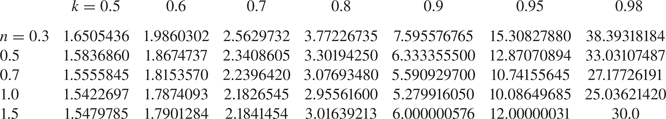
Table 3. Eigenvalues evaluated for converging radial gravity flow for different fluid behaviour index  $n$.
$n$.
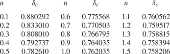
Appendix B. Flow in a porous medium of varying permeability and porosity and Hele-Shaw analogy
Consider a plane gravity current of a PL fluid propagating on a horizontal impermeable bottom toward the origin of a porous domain saturated by a lighter fluid at rest; motion is driven by the density difference  $\Delta \rho$ between the two fluids. The current is released at a distance $x_0$ from the origin and reaches it at time $t_c$. Under the assumptions of (i) sharp interface, (ii) thin intruding current, (iii) negligible capillarity effects, the spreading is described by the current height $h(x,t)$, vertical velocities are neglected, and pressure is hydrostatic with $\partial p/\partial x=\Delta \rho g(\partial h/\partial x)$. The porous domain is heterogeneous with deterministic variations in permeability $k$ and porosity $\phi$ along the horizontal direction $x$ given by
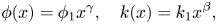 \begin{equation} \phi(x)=\phi_{1} x^{\gamma},\quad k(x)=k_{1} x^{\beta}, \end{equation}
where  $\phi _1$, $k_1$ are constants of dimensions $[L^{-\gamma }]$ and $[L^{2-\beta }]$, respectively, and $\gamma$, $\beta$ are dimensionless non-negative constants; for a homogeneous medium $\gamma =\beta =0$.
The filtration law for the PL fluid described by (2.1) is given by (Di Federico et al. Reference Di Federico, Longo, Chiapponi, Archetti and Ciriello2014)
 \begin{equation} \boldsymbol{\nabla} p-\rho {\boldsymbol{g}}={-}\frac{1}{\varLambda k^{(n+1)/2}}\left|{\boldsymbol{v}}\right|^{n-1}{\boldsymbol{v}};\quad \varLambda=\varLambda(\phi,\mu_0,n)=\frac{8^{(n+1)/2}}{2}\left(\frac{n}{3n+1}\right)^n\frac{\phi^{(n-1)/2}}{\mu_0} \end{equation}
with  $p$ the pressure, ${\boldsymbol {g}}$ gravity and ${\boldsymbol {v}} \equiv (u,v,w)$ the Darcy velocity. The mass balance for 1-D flow reads
 \begin{equation} \frac{\partial}{\partial x}\left(\int_0^hu\,\textrm{d}z\right)={-}\frac{\partial}{\partial t}\left(\int_0^h\phi\,\textrm{d}z\right). \end{equation}
Substituting the horizontal velocity from (B2) into (B3) and using (B1) yields
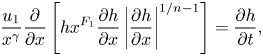 \begin{equation} \dfrac{u_1}{x^{\gamma}}\dfrac{\partial}{\partial x}\left[hx^{F_1}\dfrac{\partial h}{\partial x}\left|\dfrac{\partial h}{\partial x}\right|^{1/n-1}\right]=\dfrac{\partial h}{\partial t}, \end{equation}
with
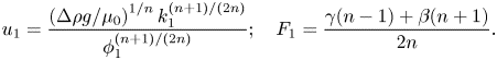 \begin{equation} u_1=\dfrac{\left(\Delta\rho g / \mu_0 \right)^{1/n}k_1^{(n+1)/(2n)}}{\phi_1^{(n+1)/(2n)}};\quad F_1=\dfrac{\gamma(n-1)+\beta(n+1)}{2n}. \end{equation}
The problem thus stated is amenable to a self-similar solution of the second kind analogous to that described in § 2 for converging flow in a channel of variable gap thickness. The dimensional counterpart of (B4) for channel flow is easily derived from (2.2) and (2.3) as
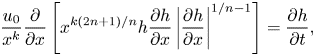 \begin{equation} \frac{u_0}{x^k}\frac{\partial}{\partial x}\left[x^{k(2n+1)/n}h\frac{\partial h}{\partial x}\left|\frac{\partial h}{\partial x}\right|^{1/n-1}\right]=\frac{\partial h}{\partial t}, \end{equation}
where
 \begin{equation} u_0=\left(\frac{\varDelta\rho g}{\mu_0}\right)^{1/n}\frac{n}{2n+1}\left(\frac{b_1}{2}\right)^{(n+1)/n}. \end{equation}
Comparing exponents in (B4) and (B6) it is seen that the Hele-Shaw analogy for PL fluids (Ciriello et al. Reference Ciriello, Longo, Chiapponi and Di Federico2016) requires
 \begin{equation} \begin{cases} \gamma=k\\ \beta=3k. \end{cases} \end{equation}
Under the validity of equations (B8) the analogy is established and one can proceed as in § 2, the critical eigenvalues will be the same. The above conditions are, however, quite restrictive; a wider choice of parameter combinations is available using a mapping parameter, see appendix A.2 in Ciriello et al. (Reference Ciriello, Longo, Chiapponi and Di Federico2016).
Non-standard Hele-Shaw cells with tapered plates have been widely applied in thin-film flows and slow viscous flows with a moving boundary, see, e.g., Al-Housseiny, Tsai & Stone (Reference Al-Housseiny, Tsai and Stone2012), Dias & Miranda (Reference Dias and Miranda2013), Al-Housseiny & Stone (Reference Al-Housseiny and Stone2013) and Bongrand & Tsai (Reference Bongrand and Tsai2018). See also Morrow, Moroney & McCue (Reference Morrow, Moroney and McCue2019) where a non-standard Hele-Shaw cell configuration (tapered of rotating) was investigated aiming to improve the efficiency in controlling interfacial instabilities.


