


1. Introduction
Sretenski (Reference Sretenski1936) and Moiseev (Reference Moiseev1953) were probably the first to show that sloshing coupled with the lateral and/or angular oscillatory tank motions is characterised by the natural sloshing frequencies  $\sigma _{s,i}$, which, generally, differ from those frequencies $\sigma _i$ without that coupling. By following the Sretenski linear unforced analysis, Herczyński & Weidman (Reference Herczyński and Weidman2012) confirmed this fact for the simplest possible case without restoring (spring-related) forces applied to the rigid tank. Practically, this happens for sway motions of a floating tank. Rognebakke & Faltinsen (Reference Rognebakke and Faltinsen2003) studied these motions in an incident two-dimensional wave whose frequency is close to the lowest coupled resonant frequency. Figure 1(a,b) exemplify the Sretenski–Moiseev-type coupled mechanical systems, which were considered by Herczyński & Weidman (Reference Herczyński and Weidman2012) and Rognebakke & Faltinsen (Reference Rognebakke and Faltinsen2003), respectively. Specifically, there are no structural eigenfrequencies in these cases (considering a ‘pseudo-frozen’ contained liquid). If the forcing frequency is close to a coupled natural frequency, e.g. the lowest one $\sigma _{s,1}$, the severe resonant sloshing in these rectangular containers should be analysed within the framework of a nonlinear theory.
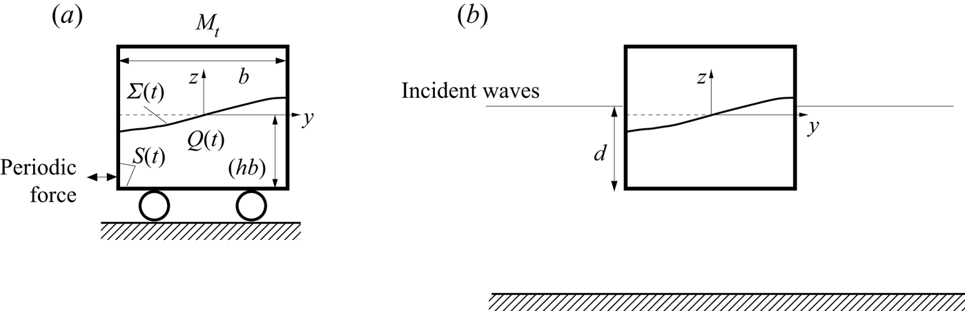
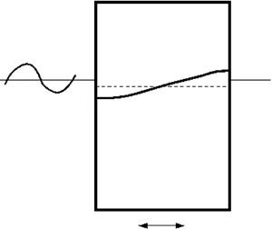
Figure 1. Two resonant sloshing problems in sloshing-affected rectangular containers, which are considered in the present paper: panel (a) depicts a resonantly forced sloshing in a rigid sloshing-affected vehicle and panel (b) sketches the swaying floating tank in incident two-dimensional waves. In these two cases, the time-dependent liquid domain  $Q(t)$, the free surface $\varSigma (t)$ and the wetted tank surface $S(t)$ are observed in the tank-fixed coordinate system $Oyz$. There is no stiffness or dashpot in the case in panel (a) as normally assumed in the Sretenski-type problem. The mechanical system is fully undamped. The damping in the case in panel (b) is not zero. In our theoretical studies, it is associated with external wave radiation and viscosity.
Nonlinear analytical sloshing theories for prescribed periodic tank motions were originated by Moiseev (Reference Moiseev1958) and further developed by Faltinsen (Reference Faltinsen1974) and Ockendon & Ockendon (Reference Ockendon and Ockendon1973). They mainly centre around steady-state resonant waves when the forcing frequency  $\sigma$ is close to the lowest natural sloshing frequency $\sigma _1$. The theories construct asymptotic solutions of the original free-surface problem and investigate their stability. Faltinsen et al. (Reference Faltinsen, Rognebakke, Lukovsky and Timokha2000) developed the so-called nonlinear multimodal method to extend the asymptotic theories on the resonant transient waves. The multimodal method establishes a link between the asymptotic steady-state wave approximation by Faltinsen (Reference Faltinsen1974) and periodic solutions of the Narimanov–Moiseev-type (modal) system of nonlinear ordinary differential equations, which couple the hydrodynamic generalised coordinates (see, Ibrahim, Pilipchuk & Ikeda (Reference Ibrahim, Pilipchuk and Ikeda2001), Ikeda (Reference Ikeda2003), Ikeda (Reference Ikeda2007), Hermann & Timokha (Reference Hermann and Timokha2005), Love & Tait (Reference Love and Tait2013) and references therein). These generalised coordinates are the time-dependent coefficients in a functional representation of the free surface by the natural sloshing modes, which are the same as the Stokes standing-wave profiles for a rectangular tank shape (Faltinsen & Timokha Reference Faltinsen and Timokha2009, chapter 4). Because the coupled natural sloshing frequencies differ from the natural sloshing (Stokes waves) frequencies without coupling, including for the lowest $\sigma _{s,1}$ and $\sigma _1$, a non-resonant sloshing can be expected when the forcing frequency $\sigma$ is close to $\sigma _1$ for the benchmark problems figure 1(a,b). As a consequence, the aforementioned analytical nonlinear theories including the multimodal Narimanov–Moiseev theory by Faltinsen et al. (Reference Faltinsen, Rognebakke, Lukovsky and Timokha2000) may fail to adequately predict resonant sloshing and its coupling with lateral motions of the two-dimensional rigid tanks.
Thus, resonant sloshing for prescribed tank motions differs from resonant sloshing coupled with lateral tank motions when the tank (rigid body) dynamics is affected by the hydrodynamic sloshing force. Resonant sloshing in the coupled systems is characterised by other linear resonance frequencies and wave profiles, which differ from the Stokes-type standing-wave solution, well known as the natural sloshing frequencies and modes in a static two-dimensional rectangular basin. A particular conclusion is that the multimodal analysis by Faltinsen et al. (Reference Faltinsen, Rognebakke, Lukovsky and Timokha2000), as well as asymptotic steady-state sloshing theories by Faltinsen (Reference Faltinsen1974) and Ockendon & Ockendon (Reference Ockendon and Ockendon1973), should then be revised by suggesting a non-Stokes modal representation of the free surface. The present paper makes the required revisions for the coupled mechanical system in figure 1(a) by deriving a novel Narimanov–Moiseev-type nonlinear modal system, constructing its steady-state (periodic) solutions, and investigating their stability. These steady-state wave results are used to analytically quantify the resonant coupling in figure 1(b) and compare the theoretical sway amplitudes with the measurements in incident regular waves by Rognebakke & Faltinsen (Reference Rognebakke and Faltinsen2003).
The coupled sloshing-vehicle dynamics in figure 1(a) is studied in § 2 by neglecting the frictional forces in connection with the wheel–rail system, assuming an inviscid incompressible liquid with two-dimensional irrotational flows, and using Lukovsky's formula for the horizontal hydrodynamic sloshing force (see, Lukovsky (Reference Lukovsky2015), Faltinsen & Timokha (Reference Faltinsen and Timokha2009), chapters 7, 8 and (2.5)). There is a given periodic lateral excitation force, which causes a resonant non-prescribed response of both the swaying tank and sloshing. Keeping the fully nonlinear statement, the Lukovsky formula makes it possible to decouple the free-surface sloshing problem from the Newton law governing the horizontal vehicle motions. The decoupled sloshing problem is formulated with respect to the free-surface elevations by  $z=\zeta (y,t)$ and the relative velocity potential $\phi (y,z,t)$ defined in the body-fixed coordinate system $Oyz$. It does not have any vehicle-related components but contains an extra integral term and external (periodic) force (applied to the body) in the dynamic boundary condition on the free surface. When the external periodic force is zero, solutions of the derived (and linearised) free-surface problem consists of a superposition of non-Stokes standing waves whose frequencies coincide with the coupled eigenfrequencies. The waves (hereafter, the non-Stokes natural sloshing modes and frequencies) are analytically derived from the corresponding spectral boundary problem. The non-Stokes natural sloshing frequencies coincide with those by Herczyński & Weidman (Reference Herczyński and Weidman2012) who obtained the frequencies from the fully coupled linear tank-sloshing statement and analytical results by Faltinsen & Timokha (Reference Faltinsen and Timokha2009, chapter 5) who derived the sloshing-related frequency-dependent added-mass coefficient. The non-Stokes frequencies and modes are functions of the non-dimensional liquid depth $h$ and the ratio $M_t/M_l$ between the tank $M_t$ and liquid $M_l$ masses.
The next subsections in § 2 construct linear and nonlinear modal theories, which are based on the non-Stokes natural sloshing modes. In the linear case, the infinite-dimensional modal equations adopting either Stokes or non-Stokes modal representation are equivalent, mathematically and from an applied point of view. The situation changes for the resonant coupled motions, which need an adequate nonlinear theory. The main goal is the Narimanov–Moiseev-type (single dominant) nonlinear modal system, which is a generalisation of the modal system by Faltinsen et al. (Reference Faltinsen, Rognebakke, Lukovsky and Timokha2000) to the case when vehicle motions are not prescribed. The derived modal system (of nonlinear ordinary differential equations) couples not two (as in Faltinsen et al. (Reference Faltinsen, Rognebakke, Lukovsky and Timokha2000)) but an infinite number of the second- and third-order hydrodynamic generalised coordinates in terms of the dominant (lowest-order) primarily excited non-Stokes mode. When the forcing frequency  $\sigma$ is close to the lowest coupled eigenfrequency $\sigma _{s,1}$ (equals the lowest non-Stokes natural sloshing frequency), the second- and third-order generalised coordinates can be amplified due to the secondary resonance phenomenon, whose appearance is extensively discussed by Faltinsen & Timokha (Reference Faltinsen and Timokha2009, chapter 8) including in the shallow water limit. Even though the adaptive and Narimanov–Moiseev modal theories accurately quantify the steady-state sloshing for finite liquid depths ( $0.3\lesssim h$), they correctly predict the secondary resonances in the hydrodynamic system for any values of $h$. Because the derived Narimanov–Moiseev modal system couples an infinite set of the second- and third-order hydrodynamic generalised coordinates, whereas Faltinsen & Timokha (Reference Faltinsen and Timokha2001) predicts secondary resonances only in the shallow liquid limit ( $h\to 0$), coupling with the vehicle motions causes the secondary resonances along several curves in the $(h,M_t/M_l)$-plane with $h=O(1)$.
To describe the steady-state resonant sloshing in figure 1(a), which occurs due to harmonic excitations of the lowest non-Stokes natural sloshing frequency  $\sigma _{s,1}$, an asymptotic periodic solution of the Narimanov–Moiseev-type modal system is derived. Its stability is investigated by implementing the linear Lyapunov method (Faltinsen & Timokha Reference Faltinsen and Timokha2009, chapter 8). The corresponding amplitude response curves demonstrate either soft-spring or hard-spring type behaviour. The behaviour switches along a curve in the $(h,M_t/M_l)$-plane instead of at the well known critical liquid depth $h=0.3368\ldots$, which determines the switch for prescribed tank motions and/or is the limiting case for $M_t/M_l\to \infty$. Typical linear and nonlinear (undamped) steady-state response curves are shown for both the sloshing and vehicle amplitudes. Whereas the sloshing-amplitude response curves seem qualitatively similar to those by Faltinsen et al. (Reference Faltinsen, Rognebakke, Lukovsky and Timokha2000), the tank amplitude has the minimum (zero in the linear case) in a neighbourhood (exactly at) of the lowest natural Stokes frequency $\sigma _1$.
Nonlinearity and damping play an important role for experimental and numerical results by Rognebakke & Faltinsen (Reference Rognebakke and Faltinsen2003) who considered a two-dimensional flow problem with a rigid floating rectangular tank that is free to sway in incident regular waves with frequency  $\sigma$ in a wide range covering both the Stokes $\sigma _1$ and non-Stokes $\sigma _{s,1}$ lowest natural sloshing frequencies. This coupled mechanical system is schematically depicted in figure 1(b). Even though damping is neglected in the steady-state analysis of § 2, the constructed undamped periodic solutions can be employed to derive analytical expressions, which describe the coupled dynamics in the (quasi)-linear (linear sloshing + linear and nonlinear damping) and/or Narimanov–Moiseev-type (nonlinear sloshing + linear and nonlinear damping) approximations.
Analytical studies and numerical examples in § 3 centre around the experimental set-up and measured data by Rognebakke & Faltinsen (Reference Rognebakke and Faltinsen2003) when the external liquid flow can be modelled within the framework of the linear free- and body-boundary conditions of the surface wave theory. A focus is on the frequency-domain problem. Various numerical solvers exist to effectively compute the corresponding frequency-dependent sway added mass  $A_{22}(\sigma )$, wave-radiation damping $B_{22}(\sigma )$ and the horizontal wave-excitation force ${F}_0(\sigma )$ associated with the external flows. We adopt the numerical coefficients from computations by Rognebakke & Faltinsen (Reference Rognebakke and Faltinsen2003).
Along with the wave-radiation damping coefficient  $B_{22}$, one should account for the nonlinear viscous damping caused by external drag forces mainly due to the flow separation (increases with increasing tank amplitude) and, specifically, the nonlinear (increases with decreasing tank amplitude) frictional force caused by the bearings in the experimental equipment. The equivalent linearisation technique is used to incorporate these two damping sources into our analytical model. Another viscous damping is associated with the laminar viscous boundary layer along the inner wetted tank surface. The latter damping can be accounted for by the Narimanov–Moiseev steady-state theory, which assumes that the lowest non-Stokes natural sloshing mode dominates and, therefore, the viscous sloshing damping could be related to the damping ratio $\xi _1$ for this dominant sloshing mode. Theoretical and experimental results by Keulegan (Reference Keulegan1959) are useful to roughly estimate $\xi _1$. Damping caused by possible internal breaking waves is not considered.
Adopting the constructed asymptotic solutions for the damped steady-state sloshing in a floating body with rectangular tanks, the theoretical amplitude response curves are drawn and compared with the measured data by Rognebakke & Faltinsen (Reference Rognebakke and Faltinsen2003). The comparison outlines conclusions regarding the resonant behaviour of the floating tanks. First, the tank-related linear resonance frequency is consistent with the undamped sloshing analysis, it coincides with the lowest non-Stokes natural sloshing frequency. Second, the sloshing-related nonlinearity matters. The derived Narimanov–Moiseev-type modal system and its steady-state solutions provide a rather accurate quantification of the measured tank sway amplitudes. Third, the Narimanov–Moiseev steady-state theory detects a narrow frequency range in the experimental cases by Rognebakke & Faltinsen (Reference Rognebakke and Faltinsen2003) where all steady-state solutions are not stable. Appearance of this range is a consequence of the external frequency-dependent damping and hydrodynamic force. According to § 2, the range is absent for the undamped case. Experimental runs in this range were discussed by Rognebakke & Faltinsen (Reference Rognebakke and Faltinsen2003) as an ‘unstable situation’ by commenting that ‘the sway amplitude shifts and thus two steady-state responses take place during one run’. Alternative numerical simulations in this frequency range by Shen et al. (Reference Shen, Greco, Faltinsen and Ma2020), who used a fully nonlinear potential flow solver, also reported difficulties to achieve a clearly steady-state wave regime.
2. Resonant sloshing and its coupling with the lateral tank motions
2.1. The coupled sloshing-vehicle dynamics: two equivalent formulations
Figure 1(a) illustrates the coupled mechanical system consisting of a rigid vehicle with mass  $M_t$ containing a rectangular container with internal breadth $b$, which is partly filled by an ideal incompressible liquid (irrotational flows) with a finite liquid depth ( $h$ is the depth-to-breadth ratio). The vehicle performs horizontal oscillations affected by the sloshing-induced ${\mathcal {F}}_{slosh}(t)$ and external ${\mathcal {F}}_{ext}(t)$ forces. No restoring and frictional forces are assumed and, therefore, no stiffness and dashpot are drawn in figure 1(a). The external force ${\mathcal {F}}_{ext}(t)$ is prescribed and periodic with the circular frequency $\sigma$, which belongs to a relatively wide range covering the lowest natural (Stokes) sloshing frequency $\sigma _1=\sqrt {(g{\rm \pi} /b) \tanh ({\rm \pi} h)}$ ( $g$ is the gravity acceleration). The hydrodynamic force ${\mathcal {F}}_{slosh}(t)$ is associated with the classical sloshing (free-surface) problem ((2.2) by Faltinsen et al. (Reference Faltinsen, Rognebakke, Lukovsky and Timokha2000)), which couples the absolute velocity potential $\varPhi$, the free surface elevations and the translatorial rigid tank velocity ${\boldsymbol v}_O(t)$ (the instant angular velocity ${\boldsymbol \omega }(t)$ is zero). The latter implies that the viscous damping is neglected and, because we neglect frictional structural forces, this section considers undamped motions of the coupled mechanical system in figure 1(a). Applicability of the hydrodynamic model of ideal liquid with irrotational flows and no surface tension accounted for is extensively discussed by Faltinsen & Timokha (Reference Faltinsen and Timokha2009, chapters 2 and 4).
2.1.1. Coupling between the free-surface sloshing problem and the lateral vehicle motions
The free-surface sloshing problem by Faltinsen et al. (Reference Faltinsen, Rognebakke, Lukovsky and Timokha2000, (2.2)) is normally formulated in the tank-fixed coordinate system  $Oyz$. When the translational velocity
 \begin{equation} {\boldsymbol v}_O(t)=b \left(\dot\eta_2(t),0\right),\quad \eta_{2b}(t)=b\eta_2(t) \end{equation}
is determined by the non-dimensional generalised coordinate (sway)  $\eta _2(t)$, adopting the spatial normalisation by $b$ and introducing the $b$-scaled relative velocity potential,
 \begin{equation} \phi(y,z,t)=\varPhi(y,z,t)/b^2-y\dot\eta_2(t), \end{equation}
where  $y$ and $z$ are the non-dimensional body-fixed coordinates, transform the two-dimensional free-surface sloshing problem to the form
 \begin{equation} \left. \begin{gathered} \nabla^2\phi=0\quad \text{in}\ Q(t);\quad \frac{\partial\phi}{\partial n} =0 \quad \text{on}\ S(t),\\ \frac{\partial\phi}{\partial n} =\frac{\partial\zeta}{\partial t}/\sqrt{1+({\partial\zeta}/{\partial y})^2}\quad \text{on}\ \varSigma(t); \quad \int_{{-}l/2}^{l/2}\zeta\,\textrm{d}y =0,\\ \frac{\partial\phi}{\partial t}+ \frac 12 (\boldsymbol{\nabla}\phi)^2 + \underbrace{\bar g}_{g/b}\zeta ={-}y\ddot\eta_2(t)\quad \text{on}\ \varSigma(t), \end{gathered} \right\} \end{equation}
where  $g$ is the gravity acceleration, $z=\zeta (y,t)$ defines the free surface $\varSigma (t)$, $Q(t)$ is the time-dependent liquid domain, $S(t)$ is the wetted tank surface, which are normalised by $b$, and ${\boldsymbol n}$ is the outer normal.
Because  $\ddot \eta _2(t)$ in the dynamic boundary condition of (2.3) is unknown, one should, in addition, introduce the Newton law with respect to $\eta _2(t)$,
 \begin{equation} b (M_t+M_l)\,\ddot \eta_2 = {\mathcal{F}}_{ext}(t)+ {\mathcal{F}}_{slosh}(t), \end{equation}
where  $M_t$ is the rigid tank mass and $M_l=\rho _l V_l$ is the liquid mass ( $\rho _l$ and $V_l$ are the liquid density and volume, respectively). The present section excludes from consideration both the frictional (structural damping) and restoring forces. As for the restoring force, it is negligibly small for sway motions of a floating tank, whose studies are the primary goal of the present paper. No damping in the original formulation is a mathematical requirement of the multimodal and almost all analytical methods in sloshing problems. The methods need the linear eigensolution (natural sloshing modes and frequencies) of the (here, coupled tank-slosh) problem, which becomes mathematically impossible with non-zero damping in the mechanical system. However, the damping terms can be incorporated into the modal equations after these are derived from the undamped formulation. How to do that is demonstrated in § 3.
The sloshing-related horizontal hydrodynamic force  ${\mathcal {F}}_{slosh}(t)$ should be derived from a pressure integral over the wetted vertical tank walls, where the pressure is computed by using the Bernoulli equation in the body-fixed coordinate system (Faltinsen & Timokha Reference Faltinsen and Timokha2009, (2.60)). Alternatively, ${\mathcal {F}}_{slosh}(t)$ can be found by using the Lukovsky formula (see details in Faltinsen & Timokha (Reference Faltinsen and Timokha2009), chapter 7),
 \begin{equation} {\mathcal{F}}_{slosh}(t)={-} M_l \ddot y_C(t)={-} M_l \frac{\textrm{d}^2}{\textrm{d}t^2} \int_{Q(t)}y\, \textrm{d}Q/V_l={-}\frac{M_l}{b^2h} \int_{{-}1/2}^{1/2}y\, \frac{\partial^2}{\partial t^2}\zeta(y,t)\,\textrm{d}y, \end{equation}
which analytically expresses the horizontal hydrodynamic force in terms of the horizontal coordinate  $y_C(t)$ of the liquid mass centre.
Equations (2.3)–(2.5) govern the coupled sloshing-tank dynamics, where the three  $b$-normalised unknowns $\zeta (y,t)$, $\phi (y,z,t)$ and $\eta _2(t)$ are defined in the body-fixed coordinate system $Oyz$. The unknowns are fully coupled, i.e. $\eta _2$ is present in the free-surface problem (2.3) and $\zeta$ appears in the Newton law (2.4).
2.1.2. Decoupling the free-surface sloshing problem from  $\eta _2(t)$

Substituting the Lukovsky formula, (2.5), into (2.4) gives
 \begin{equation} \ddot \eta_2(t) = \underbrace{\frac{{\mathcal{F}}_{ext}(t)}{b(M_t+M_l)}}_{=\bar{\mathcal{F}}_{ext}(t)} - \underbrace{\frac{M_l}{(M_l+M_t)h}}_{{=}K>0} \int_{{-}1/2}^{1/2}y\, \frac{\partial^2}{\partial t^2}\zeta(y,t)\,\textrm{d}y= \bar{\mathcal{F}}_{ext}(t)-K\ddot y_C(t). \end{equation}
Furthermore, using this formula in (2.3) partly decouples (2.3)–(2.5) so that (2.3) takes the form
 \begin{equation} \left. \begin{gathered} \boldsymbol{\nabla}^2\phi=0\quad \text{in}\ Q(t);\quad \frac{\partial\phi}{\partial n} = 0 \quad \text{on}\ S(t),\\ \frac{\partial\phi}{\partial n} =\frac{\partial\zeta}{\partial t}\left/\sqrt{1+\left(\frac{\partial\zeta}{\partial y}\right)^2}\right.\quad \text{on}\ \varSigma(t); \quad \int_{{-}1/2}^{1/2}\zeta\, \textrm{d}y=0,\\ \frac{\partial\phi}{\partial t}+ \frac 12 (\boldsymbol{\nabla}\phi)^2 -\underline{K y \int_{{-}1/2}^{1/2} y \frac{\partial^2\zeta}{\partial t^2}\,\textrm{d}y}+ \bar g \zeta ={-}y\, \bar{\mathcal{F}}_{ext}(t)\quad \text{on}\ \varSigma(t), \end{gathered} \right\} \end{equation}
where  $K$ and $\bar {\mathcal {F}}_{ext}(t)$ are defined in (2.6). The free-surface (sloshing) problem (2.7) does not contain the tank-related generalised coordinate $\eta _2(t)$; it exclusively links $\zeta (y,t)$ and $\phi (y,z,t)$. The problem describes sloshing visible through a camera installed on the rigid body .
The two mathematical formulations (2.3)–(2.5) and (2.6)–(2.7) are equivalent. They describe the coupled slosh-vehicle dynamics, forced ( ${\mathcal {F}}_{ext}\not =0$) and/or unforced ( ${\mathcal {F}}_{ext}=0$). The coupled (linear) eigenfrequencies following from these mathematical formulations were, for instance, computed by Herczyński & Weidman (Reference Herczyński and Weidman2012). The linear frequency-domain problem can also be solved by employing the sloshing-related frequency-dependent sway added-mass coefficient $A_{22}^{slosh}(\sigma )$ from Faltinsen & Timokha (Reference Faltinsen and Timokha2009, (5.134)) that deduces the governing equation
 \begin{equation} \left(M_t+M_l+A_{22}^{slosh}(\sigma)\right)\ddot\eta_{2b}(t)={\mathcal{F}}_{ext}(t) \end{equation}
from the Newton law (2.4) so that the dispersion equation for computing the coupled eigenfrequencies implies the zero coefficient at  $\ddot \eta _2(t)$, i.e. $M_t+M_l+A_{22}^{slosh}(\sigma )=0$. Here, because $A_{22}^{slosh}(\sigma )\to \pm \infty$ as $\sigma \to \sigma _1\pm$, the solution $\sigma _{s,1}>\sigma _1$.
The nonlinearity of the coupled sloshing-tank dynamics is exclusively associated with the free-surface problems (2.3) and (2.7). When considering the prescribed tank motions ( $\eta _2(t)$ is known in (2.3)), one can construct analytical approximations of the nonlinear resonant sloshing problem (2.3) in terms of the Stokes standing-wave (natural sloshing) modes in the stationary two-dimensional rectangular tank (Faltinsen & Timokha (Reference Faltinsen and Timokha2009), chapter 4). An example is the Narimanov–Moiseev multimodal theory by Faltinsen et al. (Reference Faltinsen, Rognebakke, Lukovsky and Timokha2000). This and other asymptotic analytical theories require that the forcing frequency $\sigma$ is close to the first natural sloshing frequency $\sigma _1$. The closeness is the necessary condition. However, the resonance coupled eigenfrequency $\sigma _{s,1}\not =\sigma _1$ and, therefore, applying the theories to (2.3) does not guarantee they provide an accurate prediction of the resonant coupled motions.
Because the free-surface problem (2.7) is self-contained and determines the main resonant properties of the coupled tank-sloshing mechanical system ((2.6) simply returns  $\eta _2(t)$ for the given wave elevations by $\zeta (y,t)$), the coupled eigenfrequencies should be a subset of the natural sloshing frequencies following from the linearised and unforced (2.7). Moreover, the boundary value problems (2.3) and (2.7) are mathematically similar and differ only by the underlined integral term in (2.7) (in the dynamic boundary condition on $\varSigma (t)$), which is absent in (2.3). Hence, as long as we know an analytical approach to the free-surface problem (2.3) with the prescribed acceleration $\ddot \eta _2(t)$, where $\sigma$ is close to the lowest natural sloshing frequency $\sigma _1$, mathematically, the approach could be extended to the free-surface problem (2.7) with the prescribed force $\bar {\mathcal {F}}_{ext}(t)$, where $\sigma$ is close to $\sigma _{s,1}$. How to do this extension for the nonlinear multimodal approach by Faltinsen et al. (Reference Faltinsen, Rognebakke, Lukovsky and Timokha2000) will be described in the next subsections. The procedure suggests constructing the corresponding non-Stokes natural sloshing modes and frequencies, derivation of the Narimanov–Moiseev-type (single-dominant) modal system, and studying its periodic solutions, which describe the steady-state resonant sloshing coupled with lateral tank motions.
2.2. The non-Stokes natural sloshing modes and frequencies
Because the underlined integral term in (2.7) is linearly dependent on the free-surface elevation  $\zeta$, it should affect the linear sloshing including the corresponding natural frequencies and modes. To get them, one should exclude the external forcing, $\bar {\mathcal {F}}_{ext}=0$, linearise (2.7), and pose its solution as $\phi =\varphi _s(y,z)\exp (\text {i}\sigma _s t),\, \textrm {i}^2=-1$. This leads to the following spectral boundary problem:
 \begin{equation} \left. \begin{gathered} \nabla^2\varphi_s=0\quad \text{in} \ Q_0; \quad \frac{\partial \varphi_s}{\partial n}=0\quad \text{on}\ S_0; \quad \int_{\varSigma_0} \frac{\partial \varphi_s}{\partial z}\,\textrm{d}y=0,\\ -\sigma^2_s \left(\varphi_s- K y \int_{{-}1/2}^{1/2} y \frac{\partial \varphi_s}{\partial z}\,\textrm{d}y\right) +\bar g \frac{\partial \varphi_s}{\partial z}=0\quad \text{on}\ \varSigma_0, \end{gathered} \right\} \end{equation}
where  $Q_0$ is the hydrostatic (non-dimensional) liquid domain, $\varSigma _0$ is the unperturbed free surface ( $z=0$), $S_0$ is the mean wetted tank surface and $\sigma _s$ is the corresponding natural sloshing frequency.
When the coefficient  $K=0$ (sloshing does not couple the vehicle dynamics), the spectral boundary problem (2.9) transforms to the classical spectral boundary problem in a stationary tank (Faltinsen & Timokha (Reference Faltinsen and Timokha2009), chapter 4). This determines the natural Stokes sloshing modes $\varphi _m(y,z)$ and frequencies $\sigma _m$,
 \begin{align} \varphi_{m}(y,z)= \underbrace{\cos\left({\rm \pi} m(y+\tfrac 12)\right)}_{f_{m}(y)} \underbrace{\frac{\cosh({\rm \pi} m(z+h))}{\kappa_m\cosh({\rm \pi} mh)}}_{Z_{m}(z)}; \quad \sigma^2_{m}=\bar g \ \underbrace{{\rm \pi} m \tanh({\rm \pi} m h)}_{\kappa_m},\ m\ge 1, \end{align}
which are documented, e.g. in Faltinsen & Timokha (Reference Faltinsen and Timokha2009, § 4.3.1.1).
When  $K\not =0$, the natural sloshing modes $\varphi _{s,m}(y,z)$ and frequencies $\sigma _{s,m}$ by (2.9) coincide with (2.10) for even (symmetric) wave profiles, i.e. $\varphi _{s,2i}(y,z)=\varphi _{2i}(y,z)$ and $\sigma _{s,2i}^2=\sigma _{2i}^2$ but the antisymmetric sloshing modes $\varphi _{s,2i-1}(y,z)$ and frequencies $\sigma _{s,2i-1}$ modify and become functions of $K$. The modified $\varphi _{s,2i-1}(y,z)$ and $\sigma _{s,2i-1}$ can be derived by using the harmonic functional basis (2.10) and the Treftz method, which employs the ‘antisymmetric ansatz’,
 \begin{equation} \varphi_{s,2k-1}(y,z)=\sum_{i=1}^N a_i \varphi_{2i-1}(y,z)=\sum_{i=1}^N a_i f_{2i-1}(y) Z_{2i-1}(z),\ N\to\infty. \end{equation}
The ansatz automatically satisfies the Laplace equation and the zero-Neumann condition on  $S_0$. Substituting (2.11) into the spectral boundary condition on $\varSigma _0$ in (2.9), multiplying it by $f_{2k-1}(y), k=1,\ldots ,N$ and integrating over the mean free surface leads to the spectral matrix problem
 \begin{equation} \left[\bar g I-\sigma^2_s \underbrace{(D-K\, M)}_{{\mathcal{M}}}\right] {\boldsymbol a}={\boldsymbol 0}, \end{equation}
where  ${\boldsymbol a}=(a_1,\ldots ,a_N)$ is the eigenvector, $I$ is the unit (identity) matrix, $D=\text {diag} \{ \kappa _{2m-1}^{-1}\}$, and
 \begin{equation} M=\left\{ 2 \int_{{-}1/2}^{1/2} y \,f_{2m-1}(y)\,\textrm{d}y \int_{{-}1/2}^{1/2} y \,f_{2i-1}(y)\,\textrm{d}y \right\} =\left\{ \frac{8}{{\rm \pi}^4} \frac{1 }{(2m-1)^2(2i-1)^2} \right\}. \end{equation}
Because the mass-matrix  ${\mathcal {M}}$ is symmetric, the spectral matrix problem (2.12) has the real eigenspectrum $\{\sigma _{s,2k-1}^2,\, k=1,\ldots ,N\}$.
Let  $\sigma _s^2$ be a fixed eigenvalue corresponding to the eigenvector ${\boldsymbol a}=(a_1,\ldots ,a_N)$. By introducing the auxiliary real parameter $\mu =\sum _{i=1}^N {a_i}/{(2i-1)^{2}}$ and, using the $N$ rows in the matrix problem (2.12), derives the non-zero eigenvector as follows:
 \begin{equation} {\boldsymbol a}=\left(a_m={-}K\mu \frac{8}{{\rm \pi}^4} \frac{\kappa_{2m-1} \sigma_s^2 }{(2m-1)^2 (\sigma_{2m-1}^2-\sigma_s^2)},\ m=1,\ldots,N \right) \Rightarrow \mu\not=0. \end{equation}
Inserting  $\{ a_m\}$ into the ansatz (2.11) gives the desired non-Stokes natural sloshing mode , which corresponds to the frequency $\sigma _s$.
To find the corresponding non-Stokes sloshing frequency  $\sigma _s$, one should substitute (2.14) into the expression for $\mu$. This derives the dispersion equation
 \begin{equation} {\mathcal{S}}(\sigma_s^2)= 1+K \frac{8}{{\rm \pi}^3 } \sum_{i=1}^N \frac{\sigma_s^2 \tanh({\rm \pi} (2i-1) h)}{(2i-1)^3 (\sigma_{2i-1}^2-\sigma_s^2)}=0,\quad N\to\infty, \end{equation}
which is mathematically equivalent to the zero-determinant condition (2.12).
The non-Stokes natural sloshing frequencies by (2.15) are the eigenfrequencies of the original coupled tank-sloshing system. As a consequence, the dispersion equation (2.15) is, to within the introduced notations, identical to Herczyński & Weidman (Reference Herczyński and Weidman2012, (3.8)) who analysed these coupled eigenfrequencies by using a direct integration of the pressure over the tank wall and have validated the dispersion relation by experiments. The dispersion relation looks a rather obvious consequence from expression on the sloshing-related sway added-mass coefficient  $A_{22}^{slosh}(\sigma )$ by Faltinsen & Timokha (Reference Faltinsen and Timokha2009, (5.134)). The coupled eigenfrequencies correspond to zeros of the summarised mass $M_t+M_l+A_{22}^{slosh}(\sigma )=0$, which is the same as $(M_t+M_l){\mathcal {S}}(\sigma ^2)=0$.
Our derivations of (2.15) are based on the spectral boundary problem (2.9), which deals exclusively with sloshing and has no tank-related degree of freedom. That is why they may look a little bit unusual and even complicated. Most studies are based on the fully coupled linearised problem (2.3)–(2.5). However, our goal is the non-Stokes natural sloshing modes and matrices  $D$ and ${\mathcal {M}}$, which will further be extensively employed in nonlinear sloshing theories. These theories are not derivable from (2.3)–(2.5), they need the partial decoupling, i.e. eliminating $\eta _2(t)$ from the free-surface sloshing problem.
2.2.1. Frequencies $\sigma _{s,m}$

The dispersion equation (2.15) expresses balance between inertial forces of the rigid tank + frozen liquid mechanical system and the hydrodynamic sloshing forces. In the limit  $N\to \infty$, it has an infinite set of positive real roots $\{\sigma _{s,2k-1}^2,\, k\ge 1\}$, which satisfy
 \begin{align} \sigma^2_{2i-1}<\sigma^2_{s,2i-1}<\sigma^2_{2i+1},\quad i=1,2,\ldots \quad \text{and}\quad \sigma^2_{s,2i-1}/\sigma^2_{2i-1}\to 1+\quad \text{as} \ i\to \infty. \end{align}
Because the even (symmetric) sloshing modes are not coupled with lateral tank motions in the linear approximation,
 \begin{equation} \sigma^2_{2i}=\sigma^2_{s,2i}, \quad i=1,2,\ldots . \end{equation}
However, the symmetric sloshing modes play an important role in the nonlinear resonant sloshing theories.
The theoretical ratios  $\sigma _{s,1}/\sigma _1$ and $\sigma _{s,3}/\sigma _3$ between the non-Stokes and Stokes natural sloshing frequencies are shown in figure 2(a) versus $M_t/M_l$ for three finite liquid depths $h$. The figure illustrates that the ratios tend to one with increasing $M_t/M_l$ (heavyweight tank) and $h$ (deep water). Herczyński & Weidman (Reference Herczyński and Weidman2012) have experimentally investigated $\sigma _{s,1}$ and $\sigma _{s,3}$ versus $M_l/M_t$ by varying the tank filling and compared them with the theoretical values by (2.15). Because $h$ and $M_l/M_t=[M_l/M_t](h)$ changes in a complex way in these experiments, we were not able, technically, to incorporate the measured values in figure 2(a). On the other hand, comparison by Herczyński & Weidman (Reference Herczyński and Weidman2012) confirms a good agreement between the theoretical formula (2.15) and the experimental data.

Figure 2. Natural sloshing frequencies and modes for the two-dimensional coupled sloshing-rectangular tank motion problem illustrated in figure 1(a). Panel (a) shows the two lowest antisymmetric non-Stokes natural sloshing frequencies normalised by the corresponding Stokes natural sloshing frequencies,  $\sigma _{s,1}/\sigma _1$ (the solid lines) and $\sigma _{s,3}/\sigma _3$ (the dashed deep-blue lines) versus the tank-liquid mass ratio $M_t/M_l$ for three non-dimensional liquid depths $h=0.3, 0.5$ and 0.7 (the $h$-values are used as the curves labels). Panels (b,c) compare the non-Stokes ( $z=f_{s,1}(y)$ and $=f_{s,3}(y)$ by (2.22), the deep-blue dashed lines) and Stokes ( $z=f_1(y)$ and $=f_3(y)$, the bold black solid lines) standing wave profiles for different $M_tM_l$ and $h$. Panel (b) focuses on the weightless tank ( $M_t/M_l=0$); the curves are marked by the $h$ values. The mean liquid depth $h=0.5$ is adopted in panel (c), the curves are tagged by the $M_t/M_l$ values.
2.2.2. Modes $\varphi _{s,m}$

Because of (2.14), each natural sloshing frequency  $\sigma _{s,2m-1},\, m=1,\ldots ,N$ determines the corresponding eigenvector $\boldsymbol {a}^{(2m-1)}$ whose scalar elements can be written down as
 \begin{equation} a_i^{(2m-1)}=\frac{\tanh({\rm \pi} (2i-1)h)}{(2i-1)(\sigma_{2i-1}^2/\sigma_{s,2m-1}^2-1)}, \quad i=1,\ldots,N. \end{equation}
When normalising these eigenvectors by  $\|\boldsymbol {a}^{(2m-1)}\|=\sqrt {\sum _{i=1}^N (a_i^{(2m-1)})^2}$ (the sum converges as $N\to \infty$), one can introduce the orthonormal eigenbasis
 \begin{align} {\boldsymbol q}^{(m)}= \frac{\boldsymbol{a}^{(2m-1)}}{\|\boldsymbol{a}^{(2m-1)}\|}=(q_1^{(m)}, q_2^{(m)},\ldots, q_N^{(m)})=(q_{1m}, q_{2m},\ldots,q_{Nm}),\quad m=1,\ldots,N \end{align}
so that the orthogonal matrices  $Q=\{q_{im}\}$ and $Q^T$ ( $Q^TQ=I$) diagonalise the mass-matrix ${\mathcal {M}}$, i.e.
 \begin{equation} Q^T{\mathcal{M}}Q=\text{diag} \left(\frac{1}{\kappa_{s,2k-1}}\right), \quad \text{where}\ \kappa_{s,2k-1}=\frac{\sigma^2_{s,2k-1}}{\bar g}. \end{equation}
Employing the eigenvectors (2.19) in (2.11) introduces
 \begin{equation} \varphi_{s,2m-1}(y,z)=\sum_{i=1}^N q_{im} f_{2i-1}(y) Z_{2i-1}(z),\quad N\to\infty, \end{equation}
which defines the corresponding (orthogonal) antisymmetric non-Stokes standing wave profiles
 \begin{equation} f_{s,2m-1}(y)=\left.\frac{\partial\varphi_{s,2m-1}}{\partial z}\right|_{z=0}=\sum_{i=1}^N q_{im} f_{2i-1}(y),\quad N\to \infty. \end{equation}
Specifically, the mean square root integral over  $f_{2m-1}(y)$ and $f_{s,2m-1}(y)$ are equal, i.e. $\|\,f_{2m-1}\|= \|\,f_{s,2m-1}\|=1/\sqrt {2}$. The standing antisymmetric Stokes wave profiles $f_{2m-1}(y)$ can be restored from $f_{s,2m-1}(y)$ by using $Q$ as follows:
 \begin{equation} f_{2i-1}(y)=\sum_{m=1}^N q_{im} f_{s,2m-1}(y),\quad N\to \infty. \end{equation}
 The symmetric natural sloshing modes coincide with the Stokes modes,  $\varphi _{s,2m}=\varphi _{2m}$.
The black solid lines in figure 2(b,c) show the Stokes standing wave profiles  $z=f_{1}(y)$ and $z=f_{3}(y)$, which are defined by (2.10). These wave profiles do not depend on the non-dimensional parameters $h$ and $M_t/M_l$. The antisymmetric non-Stokes wave profiles $z=f_{s,1}(y)$ and $z=f_{s,3}(y)$ by (2.22) are functions of $h$ and $M_t/M_l$.
Figure 2(b) focuses on the weightless vehicle,  $M_t/M_l=0$. The dashed curves $z=f_{s,1}(y)$ and $z=f_{s,3}(y)$ are labelled by the non-dimensional mean liquid depths ${h=0.3, 0.4, 0.7}$ and 1.5. Figure 2(c) assumes that the mean liquid depth $h$ is fixed ( $h=0.5$ in these numerical examples) but the wave profiles $z=f_{s,1}(y)$ and $z=f_{s,3}(y)$ are drawn for $M_t/M_l=0.0, 0.5, 1.0$ and 3.0 (the values are used as the tags).
Comparisons in figure 2(b,c) demonstrate that the non-Stokes natural sloshing modes are increasingly affected by the vehicle sway motions with decreasing  $h$ and $M_t/M_l$. It is most clearly seen for the lowest sloshing mode $z=f_{s,1}(y)$. An interesting feature of the non-Stokes standing wave profiles $z=f_{s,1}(y)$ and $z=f_{s,3}(y)$ is that, in contrast to the Stokes wave modes, the high spot point is situated away from the wall. Similar linear ‘high-spot’ results for the Stokes natural sloshing modes are well known for the ice-fishing problem and tanks with non-vertical walls (Kulczycki & Kuznetsov Reference Kulczycki and Kuznetsov2009, Reference Kulczycki and Kuznetsov2011). These are not connected with the flip-through phenomenon, which is of strongly nonlinear nature. As we can see, the coupling also causes the high spot point away from the wall for rectangular tanks with upright walls.
2.3. Adaptive weakly nonlinear modal equations
Faltinsen & Timokha (Reference Faltinsen and Timokha2001, (3.1)) derived a series of adaptive nonlinear modal systems (of ordinary differential equations), which couple the hydrodynamic generalised coordinates  $\beta _i(t)$ in the modal representation of the free surface by the Stokes modes,
 \begin{equation} \zeta(y,t)=\sum_{i=1}^{2N} \beta_i(t) f_i(y),\quad N\to\infty. \end{equation}
The derivations assumed prescribed tank motions (the generalised coordinate)  $\eta _2(t)$ in the variational statement of (2.3). When following these derivations for non-prescribed tank motions, the underlined integral in the free-surface problem (2.7), with the given function $\bar {\mathcal {F}}_{ext}(t)$ instead of $\ddot \eta _2(t)$ in (2.3), adds extra linear terms to the ‘odd’ modal equations governing the antisymmetric natural sloshing modes so that the aforementioned adaptive modal equations take the form
 \begin{gather} \sum_{i=1}^N \mu_{mi}\ddot\beta_{2i-1} +\bar g \beta_{2m-1} +\kappa_{2m-1}^{{-}1}N_{2m-1}=\lambda_{m}\bar{\mathcal{F}}_{ext}(t),\quad m=1,\ldots,N, \end{gather}
 \begin{gather} \ddot\beta_{2m} +\sigma_{2m}^2\beta_{2m}+ N_{2m}=0,\ \ m=1,\ldots,N, \end{gather}
where
 \begin{align} N_k=\sum_{a,b=1}^{2N} d^{1,k}_{a,b} \ddot\beta_a \beta_b +\sum_{a,b,c=1}^{2N} d^{2,k}_{a,b,c} \ddot\beta_a \beta_b \beta_c +\sum_{a,b=1}^{2N} t^{0,k}_{a,b} \dot\beta_a \dot\beta_b +\sum_{a,b,c=1}^{2N} t^{1,k}_{a,b,c} \dot\beta_a \dot\beta_b\beta_c+\ldots \end{align}
are the nonlinear components (Faltinsen & Timokha (Reference Faltinsen and Timokha2001) give explicit formulae for the  $h$-dependent hydrodynamic coefficients $d^{1,k}_{a,b}, d^{2,k}_{a,b,c}, t^{0,k}_{a,b}$, $t^{1,k}_{a,b,c},$ etc. up to the fifth polynomial terms by the generalised coordinates $\beta _i$). Furthermore,
 \begin{equation} \lambda_m={-}2\int_{{-}1/2}^{1/2} y f_{2m-1}(y)\,\textrm{d}y = \frac{4}{ {\rm \pi}^{2} (2m-1)^{2}} \end{equation}
and
 \begin{equation} \mu_{mi}=\frac{\delta_{mi}}{\kappa_{2m-1}}-K\frac{8}{{\rm \pi}^4} \frac{1 }{(2m-1)^2(2i-1)^2} \end{equation}
( $\delta _{mi}$ is the Kronecker delta) are elements of the symmetric mass-matrix ${\mathcal {M}}=\{\mu _{mi}\}$, which was introduced in (2.12).
When  $K=0$, the mass-matrix ${\mathcal {M}}$ becomes diagonal and, multiplying (2.25) by $\kappa _{2m-1}$ leads to (3.1) by Faltinsen & Timokha (Reference Faltinsen and Timokha2001) in which linear components by the hydrodynamic generalised coordinates are decoupled and $\ddot \eta _2(t)$ appears instead of ${\mathcal {F}}_{ext}(t)$. For the coupled motions, $K=M_l/(h(M_l+M_t))\not =0$ and, therefore, the mass-matrix ${\mathcal {M}}$ is not diagonal. As a consequence, the linear components in (2.25) remain coupled.
The decoupling with  $K=0$ played the fundamental role in all analytical nonlinear resonant sloshing theories. It means, in particular, that, when the forcing frequency $\sigma$ is close to the lowest natural sloshing $\sigma _1$, the only lowest natural Stokes mode has the lowest-order (dominant) asymptotic order $O(\epsilon ^{1/3})$. The lowest Fourier harmonic of the lowest hydrodynamic generalised coordinate $\beta _1(t)$ can be chosen as the lowest-order approximation of the steady-state sloshing. When $\sigma \to \sigma _{s,1}$ and $K\not =0$ in (2.25) and because of the linear coupling, an infinite set of the Stokes natural sloshing modes (generalised coordinates $\beta _{2m-1}(t)$) have the lowest Fourier harmonic of the order $O(\epsilon ^{1/3})$. There is not a clear single-dominant mode and the existing asymptotic schemes become inapplicable.
Adopting the multimodal language, appropriate revisions of these theories for the rectangular tank should be associated with replacement of (2.24) by
 \begin{equation} \zeta(y,t)=\sum_{i=1}^{N} b_{2i}(t) f_{2i}(y)+\sum_{i=1}^{N} b_{2i-1}(t) f_{s,2i-1}(y),\quad N\to\infty, \end{equation}
which employs the orthogonal functional set (2.22) by the non-Stokes natural sloshing modes and the generalised coordinates  $b_i(t),\, i=1,\ldots ,2N$ instead of $\beta _{i}(t),\, i=1,\ldots ,2N$. Formulae (2.22) and (2.23) show that transition from (2.24) to (2.29) and back is associated with algebraic operations involving the already introduced orthogonal matrices $Q$ and $Q^T$ by (2.19). In terms of $b_i(t),\, i=1,\ldots ,2N$ and $\beta _{i}(t),\, i=1,\ldots ,2N$,
 \begin{align} \beta_{2k-1}(t)
&=\sum_{i=1}^N q_{ki} b_{2i-1}(t) \iff b_{2k-1}(t)
=\sum_{i=1}^N q_{ik} \beta_{2i-1}(t);\notag\\
b_{2k}(i)&=\beta_{2k}(t),\ k=1,\ldots,N.
\end{align}
\begin{align} \beta_{2k-1}(t)
&=\sum_{i=1}^N q_{ki} b_{2i-1}(t) \iff b_{2k-1}(t)
=\sum_{i=1}^N q_{ik} \beta_{2i-1}(t);\notag\\
b_{2k}(i)&=\beta_{2k}(t),\ k=1,\ldots,N.
\end{align}
This means that one can obtain the desired nonlinear modal system with  $b_i(t),\, i=1,\ldots ,2N$ transforming (2.25) via algebraic operations with $Q$ and $Q^T$. Indeed, substituting $\beta _k(t)$ through $b_k(t)$ by (2.30) in all the modal equations of (2.25), (2.26) and, furthermore, multiplying (2.25a) by $Q^T$ from the left diagonalises the linear components of the entire adaptive modal system, which takes the form
 \begin{align} &\ddot b_{2m-1}
+\sigma_{s,2m-1}^2b_{2m-1}\notag\\ &\qquad +\sum_{a,b=1}^N \left(
d_{a,b}^{eo,2m-1}\ddot b_{2a}b_{2b-1}
+d_{a,b}^{oe,2m-1}\ddot
b_{2a-1}b_{2b}+t_{a,b}^{eo,2m-1}\dot b_{2a}\dot
b_{2b-1}\right)\nonumber\\ &\qquad +\sum_{a,b,c=1}^N
\left(d_{a,b,c}^{ooo,2m-1} \ddot
b_{2a-1}b_{2b-1}b_{2c-1}+t_{a,b,c}^{ooo,2m-1}\dot
b_{2a-1}\dot b_{2b-1} b_{2c-1}\right.\nonumber\\ &\qquad + \left. d_{a,b,c}^{oee,2m-1} \ddot
b_{2a-1}b_{2b}b_{2c} +d_{a,b,c}^{eoe,2m-1}\ddot b_{2a} b_{2b-1}
b_{2c}\right.\nonumber\\ &\qquad + \left. t_{a,b,c}^{eeo,2m-1}\dot b_{2a}\dot b_{2b} b_{2c-1}+
t_{a,b,c}^{oee,2m-1}\dot b_{2a-1}\dot b_{2b}
b_{2c}\right)\nonumber\\
&\quad =P_{2m-1}\bar{\mathcal{F}}_{ext}(t),\quad m=1,\ldots,N;
\end{align}
\begin{align} &\ddot b_{2m-1}
+\sigma_{s,2m-1}^2b_{2m-1}\notag\\ &\qquad +\sum_{a,b=1}^N \left(
d_{a,b}^{eo,2m-1}\ddot b_{2a}b_{2b-1}
+d_{a,b}^{oe,2m-1}\ddot
b_{2a-1}b_{2b}+t_{a,b}^{eo,2m-1}\dot b_{2a}\dot
b_{2b-1}\right)\nonumber\\ &\qquad +\sum_{a,b,c=1}^N
\left(d_{a,b,c}^{ooo,2m-1} \ddot
b_{2a-1}b_{2b-1}b_{2c-1}+t_{a,b,c}^{ooo,2m-1}\dot
b_{2a-1}\dot b_{2b-1} b_{2c-1}\right.\nonumber\\ &\qquad + \left. d_{a,b,c}^{oee,2m-1} \ddot
b_{2a-1}b_{2b}b_{2c} +d_{a,b,c}^{eoe,2m-1}\ddot b_{2a} b_{2b-1}
b_{2c}\right.\nonumber\\ &\qquad + \left. t_{a,b,c}^{eeo,2m-1}\dot b_{2a}\dot b_{2b} b_{2c-1}+
t_{a,b,c}^{oee,2m-1}\dot b_{2a-1}\dot b_{2b}
b_{2c}\right)\nonumber\\
&\quad =P_{2m-1}\bar{\mathcal{F}}_{ext}(t),\quad m=1,\ldots,N;
\end{align}
 \begin{align} &\ddot b_{2m}
+\sigma_{s,2m}^2b_{2m}\notag\\ &\qquad +\sum_{a,b=1}^N\left(
d_{2a,2b}^{1,2m}\ddot b_{2a}b_{2b} +d_{a,b}^{1q,2m}\ddot
b_{2a-1}b_{2b-1}+t_{2a,2b}^{0,2m}\dot b_{2a}\dot
b_{2b}+t_{a,b}^{0q,2m}\dot b_{2a-1}\dot b_{2b-1}
\right)\nonumber\\ &\qquad +\sum_{a,b,c=1}^N\left(\ddot
b_{2a}\left[
d_{2a,2b.2c}^{2,2m}b_{2b}b_{2c}+d_{a,b,c}^{2q,2m}b_{2b-1}b_{2c-1}\right]\right.\notag\\ &\qquad +\left.
b_{2c}\left[t_{2a,2b,2c}^{1,2m}\dot b_{2a}\dot
b_{2b}+t_{a,b,c}^{1q,2m}\dot b_{2a-1}\dot
b_{2b-1}\right]\right.\nonumber\\ &\qquad + \left.b_{2c-1}\left[
\bar d_{a,b,c}^{2q,2m}\ddot
b_{2a-1}b_{2b}+\bar t_{a,b,c}^{1q,2m}\dot b_{2a}\dot
b_{2b-1}\right]\right)=0,\quad \ m=1,\ldots,N,
\end{align}
\begin{align} &\ddot b_{2m}
+\sigma_{s,2m}^2b_{2m}\notag\\ &\qquad +\sum_{a,b=1}^N\left(
d_{2a,2b}^{1,2m}\ddot b_{2a}b_{2b} +d_{a,b}^{1q,2m}\ddot
b_{2a-1}b_{2b-1}+t_{2a,2b}^{0,2m}\dot b_{2a}\dot
b_{2b}+t_{a,b}^{0q,2m}\dot b_{2a-1}\dot b_{2b-1}
\right)\nonumber\\ &\qquad +\sum_{a,b,c=1}^N\left(\ddot
b_{2a}\left[
d_{2a,2b.2c}^{2,2m}b_{2b}b_{2c}+d_{a,b,c}^{2q,2m}b_{2b-1}b_{2c-1}\right]\right.\notag\\ &\qquad +\left.
b_{2c}\left[t_{2a,2b,2c}^{1,2m}\dot b_{2a}\dot
b_{2b}+t_{a,b,c}^{1q,2m}\dot b_{2a-1}\dot
b_{2b-1}\right]\right.\nonumber\\ &\qquad + \left.b_{2c-1}\left[
\bar d_{a,b,c}^{2q,2m}\ddot
b_{2a-1}b_{2b}+\bar t_{a,b,c}^{1q,2m}\dot b_{2a}\dot
b_{2b-1}\right]\right)=0,\quad \ m=1,\ldots,N,
\end{align}
where  $\sigma _{s,i}$ are the non-Stokes natural sloshing frequencies,
 \begin{equation} P_{2m-1} =\kappa_{s,2m-1} {\sum_{j=1}^N q_{jm} \lambda_j}=\kappa_{s,2m-1} \mu_m \end{equation}
( $\kappa _{s,2m-1}$ are defined in (2.20) and $\lambda _i$ come from (2.27)). The hydrodynamic coefficients at the nonlinear terms are computed by the following formulae:
 \begin{gather} d_{a,b}^{eo,2m-1}=\kappa_{s,2m-1}\sum_{k,i=1}^Nq_{km}q_{ib} \frac{d_{2a,2i-1}^{1,2k-1}}{\kappa_{2k-1}};\quad d_{a,b}^{oe,2m-1}=\kappa_{s,2m-1}\sum_{k,i=1}^Nq_{km}q_{ia} \frac{d_{2i-1,2b}^{1,2k-1}}{\kappa_{2k-1}}; \end{gather}
 \begin{gather} t_{a,b}^{eo,2m-1}=\kappa_{s,2m-1}\sum_{k,i=1}^Nq_{km}q_{ib} \frac{t_{2a,2i-1}^{0,2k-1}+t_{2i-1,2a}^{0,2k-1}}{\kappa_{2k-1}}; \end{gather}
 \begin{gather} d_{a,b,c}^{ooo,2m-1}=\kappa_{s,2m-1}\sum_{k,i,j,l=1}^Nq_{km}q_{ia}q_{jb}q_{lc}\frac{d_{2i-1,2j-1,2l-1}^{2,2k-1}}{\kappa_{2k-1}}; \end{gather}
 \begin{gather} t_{a,b,c}^{ooo,2m-1}=\kappa_{s,2m-1}\sum_{k,i,j,l=1}^Nq_{km}q_{ia}q_{jb}q_{lc}\frac{t_{2i-1,2j-1,2l-1}^{1,2k-1}}{\kappa_{2k-1}}; \end{gather}
 \begin{gather} d_{a,b,c}^{oee,2m-1}=\kappa_{s,2m-1}\sum_{k,i=1}^Nq_{km}q_{ia} \frac{d_{2i-1,2b,2c}^{2,2k-1}}{\kappa_{2k-1}};\quad t_{a,b,c}^{eeo,2m-1}=\kappa_{s,2m-1}\sum_{k,i=1}^N q_{km}q_{ic} \frac{t_{2a,2b,2i-1}^{1,2k-1}}{\kappa_{2k-1}}; \end{gather}
 \begin{gather} d_{a,b,c}^{eoe,2m-1}=\kappa_{s,2m-1}\sum_{i,k=1}^Nq_{km}q_{ib} \frac{d_{2a,2i-1,2c}^{2,2k-1}+d_{2a,2l,2i-1}^{2,2k-1}}{\kappa_{2k-1}}; \end{gather}
 \begin{gather} t_{a,b,c}^{oee,2m-1}=\kappa_{s,2m-1}\sum_{k,i=1}^N q_{km}q_{ia} \frac{t_{2i-1,2b,2c}^{1,2k-1}+t_{2b,2i-1,2c}^{1,2k-1}}{\kappa_{2k-1}}; \end{gather}
 \begin{gather} d_{a,b}^{1q,2m}=\sum_{i,j=1}^Nq_{ia}q_{jb}d_{2i-1,2j-1}^{1,2m};\quad t_{a,b}^{0q,2m}=\sum_{i,j=1}^Nq_{ia}q_{jb}t_{2i-1,2j-1}^{0,2m}; \end{gather}
 \begin{gather} d_{a,b,c}^{2q,2m}=\sum_{i,j=1}^Nq_{ib}q_{jc}d_{2a,2i-1,2j-1}^{2,2m};\quad \bar d_{a,b,c}^{2q,2m}=\sum_{i,j=1}^Nq_{ia}q_{jc} (d_{2i-1,2b,2j-1}^{2,2m}+d_{2i-1,2j-1,2b}^{2,2m}); \end{gather}
 \begin{gather} t_{a,b,c}^{1q,2m}=\sum_{i,j=1}^N q_{ia}q_{jb} t_{2i-1,2j-1,2c}^{1,2m};\quad \bar t_{a,b,c}^{1q,2m}=\sum_{i,j=1}^N q_{ib}q_{jc}(t_{2a,2i-1,2j-1}^{1,2m}+t_{2i-1,2a,2j-1}^{1,2m}). \end{gather}
As long as we know a solution of the modal system (2.31), which describes an undamped resonant sloshing coupled with the tank motions, using (2.6), (2.24), (2.27), (2.30) and (2.32) derives the following linear expression for the vehicle sway acceleration
 \begin{equation} \ddot \eta_2(t) = \bar{\mathcal{F}}_{ext}(t)+ \tfrac 12 K \sum_{m=1}^N \mu_m \ddot b_{2m-1}(t), \end{equation}
where  $\mu _m$ are defined in (2.32).
2.4. The linear modal theories
The non-resonant sloshing may effectively be described by using both Stokes and non-Stokes modal representations within the framework of the linear sloshing theory, which assumes the asymptotically small external force,
 \begin{equation} \bar{\mathcal{F}}_{ext}(t) = \sigma^2 O(\epsilon), \quad \epsilon\ll 1, \end{equation}
so that the free-surface elevation and other hydrodynamic characteristics are of the same order  $O(\epsilon )$,
 \begin{equation} \eta_2\sim \beta_{m}\sim b_m =O(\epsilon),\quad m=1,2,\ldots. \end{equation}
Furthermore, the  $o(\epsilon )$-order components are neglected.
2.4.1. Two equivalent linear modal equations
Let us take the well known linear modal system from § 5.4.2 by Faltinsen & Timokha (Reference Faltinsen and Timokha2009):
 \begin{equation} \ddot \beta_{2m-1} +\sigma_{2m-1}^2 \beta_{2m-1}=\kappa_{2m-1} \lambda_m \ddot\eta_2;\quad \ddot \beta_{2m} +\sigma_{2m}^2b_{2m}=0,\quad m=1,\ldots,N. \end{equation}
Because the sway motion  $\eta _2(t)$ is unknown, using (2.46a,b) requires the Newton law (2.6), which should be rewritten in the form
 \begin{equation} \ddot\eta_2(t)=\bar{\mathcal{F}}_{ext}(t) +\frac 12 K \sum_{m=1}^N \lambda_m \ddot\beta_{2m-1}(t). \end{equation}
The system of linear ordinary differential equations (2.46a,b), (2.47) describes the linear coupled dynamics in terms of the generalised coordinates  $\eta _2$ and $\beta _{2m-1}$. The even hydrodynamic coordinates $\beta _{2m}$ do not effect the coupling and, therefore, can be excluded from the linear analysis.
Alternatively, one can focus on the linearised modal equations (2.31),
 \begin{align} \ddot b_{2m-1} +\sigma_{s,2m-1}^2b_{2m-1}=P_{2m-1}\bar{\mathcal{F}}_{ext};\quad \ddot b_{2m} +\sigma_{s,2m}^2b_{2m}=0,\quad m=1,\ldots,N. \end{align}
These equations do not contain  $\eta _2(t)$. They describe the internal wave motions, not the tank motions. However, when solving (2.48a,b) and substituting $b_{2m-1}(t)$ into (2.43), we get an explicit expression for $\ddot \eta _2(t)$.
The systems of ordinary differential equations (2.46a,b) + (2.47) and (2.48a,b) + (2.43) imply two equivalent linear modal systems, which describe the coupled dynamics. An advantage of (2.48a,b) + (2.43) is that it concentrates on sloshing but the associated tank motions by  $\eta _2(t)$ become automatically derivable (known) if we know the hydrodynamic generalised coordinates $b_{2i-1}(t)$. On the other hand, derivations of the linear modal equations (2.48a,b) require knowledge of the non-Stokes sloshing frequencies $\sigma _{s,2i-1}$ and matrix $Q$ while the hydrodynamic coefficients in (2.46a,b) + (2.47) can be computed by using rather simple analytical formulae.
2.4.2. Steady-state wave motions
The steady-state linear analysis suggests the small-amplitude harmonic force
 \begin{equation} \bar{\mathcal{F}}_{ext}(t)=\sigma^2f_0\cos\sigma t,\quad 0\not=f_0=O(\epsilon)\ll 1. \end{equation}
Substituting (2.49) into either (2.46a,b) + (2.47) or/and (2.48a,b) + (2.43) derives the two equivalent periodic (steady-state) solutions in terms of  $\beta _{2m-1}$ or/and $b_{2m-1}$,
 \begin{align} \beta_{2m-1}(t)=\beta_{0,2m-1}\cos\sigma t;\quad b_{2m-1}(t)=b_{0,2m-1}\cos\sigma t;\quad \eta_2(t)=a_t\cos\sigma t, \end{align}
where
 \begin{equation} \beta_{0,2m-1}={-}\frac{\sigma^2 \kappa_{2m-1}\lambda_m}{\sigma_{2m-1}^2-\sigma^2}a_t;\quad b_{0,2m-1}=\frac{\sigma^2 P_{2m-1}}{\sigma_{s,2m-1}^2-\sigma^2}f_0. \end{equation}
Furthermore, (2.46a,b) + (2.47) gives the transmission function for the sway amplitude  $a_t$:
 \begin{equation} \frac{a_t}{f_0} ={-} \frac{1}{S(\sigma^2)}, \end{equation}
where the function  $S(\sigma ^2)$ was introduced when defining the dispersion equation (2.15). An alternative expression of the dispersion function is also derivable when using the linear modal equations (2.48a,b) + (2.43); the result is
 \begin{equation} -\frac {1}{S(\sigma^2)} ={-}1 +\frac 12 K \sum_{m=1}^N \frac{\mu_m^2 \kappa_{s,2m-1}}{\bar\sigma_{s,2m-1}^2-1},\quad \bar\sigma_{s,2m-1}=\frac{\sigma_{s,2m-1}}{\sigma}. \end{equation}
The key difference between (2.15) and (2.53) is that the first expression employs the Stokes natural sloshing frequencies  $\sigma _{2m-1}$ but the second one is based on the non-Stokes natural sloshing frequencies $\sigma _{s,2m-1}$.
When the forcing frequency  $\sigma$ tends to $\sigma _{s,2m-1}$, the second formula in (2.51a,b) and (2.52) ( $S(\sigma ^2)\to 0$ as $\sigma ^2\to \sigma _{s,2m-1}^2$) show that both the amplitude $b_{0,2m-1}$ (of the hydrodynamic generalised coordinate $b_{2m-1}$) and the tank amplitude $a_t$ tend to infinity. In other words, $\sigma _{s,2m-1}$ is the resonant frequency for both the liquid and vehicle motions.
When the forcing frequency  $\sigma$ tends to the Stokes natural sloshing frequency $\sigma _{2m-1}$, ( $S(\sigma ^2)\to \infty$ according to (2.15)), and, therefore, the tank amplitude $a_t$ tends to zero according to (2.52). This limit explains why $\sigma _{2m-1}$ are not the resonance sloshing frequencies anymore, even though the first formula in (2.51a,b) has the denominator $\sigma _{2m-1}^2-\sigma ^2$. Inserting $a_t$ from (2.52) into the formula for $\beta _{0,2m-1}$ in (2.51a,b) and using L’Hôpital's rule proves that $\beta _{0,2m-1}\to {\rm \pi}^2 (2m-1)^2 f_0 /(2K)$ as $\sigma \to \sigma _{2m-1}$, i.e. the sloshing amplitude is finite at the Stokes resonance frequencies unless $M_t/M_l\to \infty$.
Coupling between steady-state sloshing and tank motions introduces both the vehicle and sloshing amplitudes. The vehicle amplitude is associated with  $\mbox {max}\, |\eta _2(t)|$, which is, in the linear case, the same as $|a_t|$ (the modulus of the first Fourier harmonic). Because the Stokes natural sloshing modes reach the high spot on the wall, the sloshing amplitude can be associated with max $|\sum \beta _i(t)|$ in terms of the modal representation (2.24) (the maximum wave elevation at the wall). Figure 2(b,c) demonstrates that the high-spot point of $z=f_{s,2m-1}(y)$ is not on the wall and, therefore, analogous direct sum by $b_i(t)$ cannot be used as definition of the sloshing amplitude when adopting (2.29). An alternative definition of the sloshing amplitude could be associated with the $b$-normalised amplitude of the liquid mass centre in the horizontal direction (relative to the $Oyz$ frame)
 \begin{equation} \max|y_C(t)|, \quad \text{where}\ y_C(t)=\frac{1}{h}\int_{{-}1/2}^{1/2} y\zeta(y,t)\,\textrm{d}y ={-}\frac{1}{2 h}\sum_{m=1}^N \mu_m b_{2m-1}(t), \end{equation}
which is independent of the high-spot position of  $z=f_{s,2m-1}(y)$. Physically, $\ddot y_C(t)$ is by the Lukovsky formula (2.5) related to the horizontal hydrodynamic sloshing force. The position of $y_C(t)$ is utilised in phenomenological sloshing models such as the concentrated mass model by Ishikawa et al. (Reference Ishikawa, Kondou, Matsuzaki and Yamamura2016).
Substituting  $b_{2m-1}(t)$ by (2.51a,b) derives the linear steady-state liquid-mass motions in the horizontal direction
 \begin{equation} y_C(t)=a_s\cos\sigma t, \end{equation}
so that  $|a_s|$ is the sloshing amplitude in the linear case. The transmission function for $a_s$ takes the form
 \begin{equation} \frac{a_s}{f_0}={-}\frac{1}{2h} \sum_{m=1}^N \frac{\mu_m^2\kappa_{s,2m-1}}{\bar\sigma_{s,2m-1}^2-1}= \frac{M_t+M_l}{M_l}\left[\frac{1}{S(\sigma^2)}-1\right]. \end{equation}
Comparing (2.56) and (2.52) shows that amplitudes  $a_t$ and $a_s$ become infinite and change their sign at $\sigma = \sigma _{s,2m-1}$. As we discussed above, when $\sigma \to \sigma _{2m-1}$, the sway amplitude of the vehicle tends to zero but $a_s/f_0\to -(1+M_t/M_l)$. A particular consequence of the latter limit is that, if $M_t/M_l=O(1)$, $a_s\sim f_0$ at $\sigma =\sigma _{2m-1}$, and, therefore, the resonant steady-state sloshing in the small vicinity of $\sigma _1$ should be rather accurately approximated within the framework of the linear sloshing theory.
The transmission functions  $a_s/f_0$ and $a_t/f_0$ by (2.56) and (2.52), respectively, are drawn in figure 3 for $h=0.5$ and $M_t/M_l=1$. Positive values of $a_t/f_0$ and $a_s/f_0$ mean that the liquid mass centre and/or vehicle oscillate in-phase with the external harmonic forcing (2.49) but the negative values imply the out-of-phase oscillation. As usual for the linear harmonically forced oscillator, $a_s/f_0$ (the deep-blue dashed lines), the liquid mass oscillations change the phase when going through the resonance at $\sigma _{s,1}$. However, $a_t/f_0$ (the solid lines) shows that the vehicle oscillations change their phase twice, at the resonance frequency $\sigma _{s,1}$ and at the first Stokes natural sloshing frequency ( $\sigma /\sigma _{s,1}= \sigma _1/\sigma _{s,1}=0.874677\ldots$ for the chosen input data) so that the vehicle oscillates in-phase only in the interval $\sigma _1<\sigma <\sigma _{s,1}$. Why $a_t=0$ and $a_s/f_0=-1-M_t/M_l$ at $\sigma =\sigma _1$ is discussed above in the text.

Figure 3. Transmission functions  $a_t/f_0$ (the solid lines) for the tank sway amplitude and $a_s/f_0$ (the deep-blue dashed lines) for the liquid mass amplitude in the horizontal direction by (2.52) and (2.56), respectively. The computations were done with $h=0.5$ and $M_t/M_l=1$. The graphic representation demonstrates that the tank does not move but the liquid mass centre oscillates in the horizontal direction with the amplitude $-1-M_t/M_l$ when $\sigma =\sigma _1$. Positive vertical values of the transmission functions imply the in-phase oscillations with the harmonic external force $\bar {\mathcal {F}}_{ext}(t)$ by (2.49).
2.5. The Narimanov–Moiseev nonlinear modal theory
2.5.1. The single-dominant modal system
Resonant sloshing with a finite liquid depth and  $\sigma$ approaching the lowest natural sloshing frequency is normally well quantified within the framework of the so-called Narimanov–Moiseev asymptotic theory (Narimanov Reference Narimanov1957; Moiseev Reference Moiseev1958; Ockendon & Ockendon Reference Ockendon and Ockendon1973; Faltinsen Reference Faltinsen1974). Faltinsen et al. (Reference Faltinsen, Rognebakke, Lukovsky and Timokha2000) and Faltinsen & Timokha (Reference Faltinsen and Timokha2001) derived the corresponding modal system for the prescribed harmonic tank forcing.
The corresponding derivations for the modal system (2.31) start with the primarily excited generalised coordinate  $b_1(t)$, which should, according to the Narimanov–Moiseev theory, possess the lowest asymptotic order $O(\epsilon ^{1/3})$ equipped with the Moiseev-type detuning
 \begin{equation} \sigma_{s,1}^2/\sigma^2-1= O(\epsilon^{2/3}), \end{equation}
that measures the ‘closeness’ between  $\sigma$ and $\sigma _{s,1}$ in terms of $f_0=O(\epsilon )\ll 1$. Assuming $b_1(t)=O(\epsilon ^{1/3})$ and utilising symmetry/antisymmetry of the non-Stokes natural sloshing modes $f_{s,m}(y)$ leads to the following asymptotic relations:
 \begin{equation} b_1(t)=O(\epsilon^{1/3}),\quad b_{2m}(t)=O(\epsilon^{2/3}),\quad b_{2m+1}(t)=O(\epsilon),\quad m=1,\ldots,N,\ N\to\infty. \end{equation}
 Adopting (2.58a–c) and excluding the  $o(\epsilon )$-order terms yields the following system of ordinary differential (Narimanov–Moiseev-type modal) equations:
 \begin{align} &\ddot b_{1}
+\sigma_{s,1}^2 b_{1} + d_2 (\ddot b_1 b_1^2 +\dot b_1^2
b_1) +\sum_{b=1}^N \left( d_{1,b} \left[\ddot b_1 b_{2b}
+\dot b_1 \dot b_{2b} \right] + d_{3,b} b_1 \ddot b_{2b}
\right)\nonumber\\ &\quad =P_{2m-1}\bar{\mathcal{F}}_{ext}(t),
\end{align}
\begin{align} &\ddot b_{1}
+\sigma_{s,1}^2 b_{1} + d_2 (\ddot b_1 b_1^2 +\dot b_1^2
b_1) +\sum_{b=1}^N \left( d_{1,b} \left[\ddot b_1 b_{2b}
+\dot b_1 \dot b_{2b} \right] + d_{3,b} b_1 \ddot b_{2b}
\right)\nonumber\\ &\quad =P_{2m-1}\bar{\mathcal{F}}_{ext}(t),
\end{align}
 \begin{align} &\ddot
b_{2n}+\sigma_{s,2n}^2 b_{2n}+ d_4^{(n)} \ddot b_1 b_1+
d_5^{(n)} \dot b_1\dot b_1=0,\quad n=1,\ldots,N,
\end{align}
\begin{align} &\ddot
b_{2n}+\sigma_{s,2n}^2 b_{2n}+ d_4^{(n)} \ddot b_1 b_1+
d_5^{(n)} \dot b_1\dot b_1=0,\quad n=1,\ldots,N,
\end{align}
 \begin{align} &\ddot b_{2m-1}
+\sigma_{s,2m-1}^2 b_{2m-1} + d_7^{(m)} \ddot b_1 b_1^2
+d_{10}^{(m)} \dot b_1^2 b_1\notag\\ &\qquad +\sum_{b=1}^N \left(
d^{(m)}_{6,b} \ddot b_1 b_{2b} +d^{(m)}_{8,b}\ddot
b_{2b}b_1 + d_{9,b}^{(m)} \dot b_1 \dot b_{2b}
\right)\nonumber\\ &\quad =P_{2m-1}\bar{\mathcal{F}}_{ext}(t),\ \
m=2,\ldots,N. \end{align}
\begin{align} &\ddot b_{2m-1}
+\sigma_{s,2m-1}^2 b_{2m-1} + d_7^{(m)} \ddot b_1 b_1^2
+d_{10}^{(m)} \dot b_1^2 b_1\notag\\ &\qquad +\sum_{b=1}^N \left(
d^{(m)}_{6,b} \ddot b_1 b_{2b} +d^{(m)}_{8,b}\ddot
b_{2b}b_1 + d_{9,b}^{(m)} \dot b_1 \dot b_{2b}
\right)\nonumber\\ &\quad =P_{2m-1}\bar{\mathcal{F}}_{ext}(t),\ \
m=2,\ldots,N. \end{align}
The hydrodynamic coefficients at the nonlinear terms are functions of the mean liquid depth  $h$ and the mass ratio $M_t/M_l$. They are computed by the formulae
 \begin{align}
d_{1,b}&=d_{6,b}^{(1)}=d_{9,b}^{(1)}=
d_{1,b}^{oe,1}=t_{b,1}^{eo,1}= \kappa_{s,1}\sum_{k,i=1}^N
q_{k1}q_{i1} \frac{d_{2i-1,2b}^{1,2k-1}}{\kappa_{2k-1}}\notag\\ &=
\kappa_{s,1} \sum_{k,i=1}^N q_{k1}q_{i1}
\frac{t_{2b,2i-1}^{0,2k-1}+t_{2i-1,2b}^{0,2k-1}}{\kappa_{2k-1}};
d_2=d_7^{(1)}=d_{10}^{(1)}= d_{1,1,1}^{ooo,1}=t_{1,1,1}^{ooo,1}\notag\\
&=\kappa_{s,1}\sum_{k,i,j,l=1}^Nq_{k1}q_{i1}q_{j1}q_{l1}\frac{d_{2i-1,2j-1,2l-1}^{2,2k-1}}{\kappa_{2k-1}}
= \kappa_{s,1}\sum_{k,i,j,l=1}^Nq_{k1}q_{i1}q_{j1}q_{l1}\frac{t_{2i-1,2j-1,2l-1}^{1,2k-1}}{\kappa_{2k-1}};\notag\\
d_{3,b}&=d_{8,b}^{(1)}= d_{b,1}^{eo,1}=\kappa_{s,1}\sum_{k,i=1}^Nq_{k1}q_{i1}
\frac{d_{2b,2i-1}^{1,2k-1}}{\kappa_{2k-1}}; \end{align}
\begin{align}
d_{1,b}&=d_{6,b}^{(1)}=d_{9,b}^{(1)}=
d_{1,b}^{oe,1}=t_{b,1}^{eo,1}= \kappa_{s,1}\sum_{k,i=1}^N
q_{k1}q_{i1} \frac{d_{2i-1,2b}^{1,2k-1}}{\kappa_{2k-1}}\notag\\ &=
\kappa_{s,1} \sum_{k,i=1}^N q_{k1}q_{i1}
\frac{t_{2b,2i-1}^{0,2k-1}+t_{2i-1,2b}^{0,2k-1}}{\kappa_{2k-1}};
d_2=d_7^{(1)}=d_{10}^{(1)}= d_{1,1,1}^{ooo,1}=t_{1,1,1}^{ooo,1}\notag\\
&=\kappa_{s,1}\sum_{k,i,j,l=1}^Nq_{k1}q_{i1}q_{j1}q_{l1}\frac{d_{2i-1,2j-1,2l-1}^{2,2k-1}}{\kappa_{2k-1}}
= \kappa_{s,1}\sum_{k,i,j,l=1}^Nq_{k1}q_{i1}q_{j1}q_{l1}\frac{t_{2i-1,2j-1,2l-1}^{1,2k-1}}{\kappa_{2k-1}};\notag\\
d_{3,b}&=d_{8,b}^{(1)}= d_{b,1}^{eo,1}=\kappa_{s,1}\sum_{k,i=1}^Nq_{k1}q_{i1}
\frac{d_{2b,2i-1}^{1,2k-1}}{\kappa_{2k-1}}; \end{align}
 \begin{align} d^{(n)}_4&=d_{1,1}^{1q,2n}=\sum_{i,j=1}^Nq_{i1}q_{j1}d_{2i-1,2j-1}^{1,2n},\quad d^{(n)}_5=t_{1,1}^{0q,2n}=\sum_{i,j=1}^Nq_{i1}q_{j1}t_{2i-1,2j-1}^{0,2n}; \end{align}
 \begin{align} &\left. \begin{gathered} d_{6,b}^{(m)} = d_{1,b}^{oe,2m-1}=\kappa_{s,2m-1}\sum_{k,i=1}^Nq_{km}q_{i1} \frac{d_{2i-1,2b}^{1,2k-1}}{\kappa_{2k-1}},\\ d_7^{(m)} =d_{1,1,1}^{ooo,2m-1}=\kappa_{s,2m-1}\sum_{k,i,j,l=1}^Nq_{km}q_{i1}q_{j1}q_{l1}\frac{d_{2i-1,2j-1,2l-1}^{2,2k-1}}{\kappa_{2k-1}},\\ d_{8,b}^{(m)} =d_{b,1}^{eo,2m-1}=\kappa_{s,2m-1}\sum_{k,i=1}^Nq_{km}q_{i1} \frac{d_{2b,2i-1}^{1,2k-1}}{\kappa_{2k-1}},\\ d_{9,b}^{(m)} = t_{b,1}^{eo,2m-1}=\kappa_{s,2m-1}\sum_{k,i=1}^Nq_{km}q_{i1} \frac{t_{2b,2i-1}^{0,2k-1}+t_{2i-1,2b}^{0,2k-1}}{\kappa_{2k-1}},\\ d_{10}^{(m)} =t_{1,1,1}^{ooo,2m-1}=\kappa_{s,2m-1}\sum_{k,i,j,l=1}^Nq_{km}q_{i1}q_{j1}q_{l1}\frac{t_{2i-1,2j-1,2l-1}^{1,2k-1}}{\kappa_{2k-1}}. \end{gathered} \right\} \end{align}
 In contrast to the prescribed tank motions when the Narimanov–Moiseev-type modal system (Faltinsen et al. (Reference Faltinsen, Rognebakke, Lukovsky and Timokha2000), (5.24)) nonlinearly couples only three degrees of freedom,  $\beta _1(t),\beta _2(t)$ and $\beta _3(t)$, the Narimanov–Moiseev-type modal system (2.59) couples an infinite set of the second-order, $b_{2m}(t)=O(\epsilon ^{2/3})$, and third-order, $b_{2m+1}(t)=O(\epsilon ^{3/3})$, hydrodynamic generalised coordinates.
2.5.2. Steady-state resonance sloshing and its stability
Let us assume (2.49) and  $\sigma$ belong to a neighbourhood of the lowest natural sloshing frequency $\sigma _{s,1}$ so that (2.57) is satisfied. Our goal consists of constructing a steady-state wave (periodic) solution of the Narimanov–Moiseev-type modal system (2.59), studying its stability, and analysing the corresponding response curves, which are associated with either the sloshing or tank amplitudes versus the forcing frequency $\sigma$.
The primarily excited generalised coordinate  $b_1(t)$ has the lowest asymptotic order and this dominant asymptotic contribution is associated with the first Fourier harmonic, i.e.
 \begin{equation} b_1(t)=a\cos\sigma t +o(\epsilon^{1/3}),\quad a=O(\epsilon^{1/3}). \end{equation}
Substituting (2.61) into modal equations (2.59b) derives
 \begin{equation} b_{2n}(t)=a^2 (l_{0,n} +h_{0,n}\cos 2\sigma t) + o(a^3), \end{equation}
where
 \begin{equation} l_{0,n}=\frac{d_4^{(n)}-d_5^{(n)}}{2\bar\sigma_{s,2n}^2},\quad h_{0,n}=\frac{d_4^{(n)}+d_5^{(n)}}{2(\bar\sigma_{s,2n}^2-4)},\quad \bar\sigma_{s,i}=\frac{\sigma_{s,i}}{\sigma}. \end{equation}
Inserting (2.61) and (2.62) into (2.59a) and gathering all quantities at the first harmonic yields the cubic secular (solvability) condition, which couples the forcing frequency  $\sigma$, the forcing amplitude $f_0$ and the dominant sloshing amplitude $a$ as follows:
 \begin{equation} a \left(\varLambda(\sigma^2) + m_1a^2\right) =P_1 f_0=\varepsilon=O(\epsilon),\quad \varLambda(\sigma^2)= \bar\sigma_{s,1}^2-1, \end{equation}
where  $P_1$ is defined in (2.32) and
 \begin{equation} m_1={-}\tfrac 12 d_2 + \sum_{i=1}^N \left( d_{1,i} \left[{-}l_{0,i} +\tfrac 12 h_{0,i}\right] -2 d_{3,i}h_{0,i}\right). \end{equation}
 Furthermore, assuming  $a$ is found from the secular condition (2.64) and gathering the corresponding asymptotic terms in (2.59a) up to the $O(\epsilon )$ order derives
 \begin{equation} b_1(t)=a\cos\sigma t + a^3 \frac{N_{2,1}}{\bar\sigma_{s,1}^2-9} \cos 3\sigma t + o(a^3). \end{equation}
Making the same operation with (2.59c) gives the third-order approximation
 \begin{align} b_{2m-1}(t)=\frac{P_{2m-1}f_0-N_{1,m}a^3}{\bar\sigma_{s,2m-1}^2-1}\cos\sigma t + a^3 \frac{N_{2,m}}{\bar\sigma_{s,2m-1}^2-9} \cos 3\sigma t + o(a^3),\quad m\ge 2, \end{align}
where
 \begin{equation} \left. \begin{gathered} N_{1,m}={-}\frac 34 d_7^{(m)}+\frac 1 4 d_{10}^{(m)} +\sum_{i=1}^N \left[ h_{0,i}\left( -\frac 12 d_{6,i}^{(m)}-2d_{8,i}^{(m)}+d_{9,i}^{(m)}\right) -l_{0,i}d_{6,i}^{(m)}\right],\\ N_{2,m}= \frac 14 d_7^{(m)}+\frac 1 4 d_{10}^{(m)}+\sum_{i=1}^N h_{0,i}\left( \frac 12 d_{6,i}^{(m)}+2d_{8,i}^{(m)}+d_{9,i}^{(m)}\right). \end{gathered} \right\} \end{equation}
Specifically, according to the relations between the hydrodynamic coefficients (2.60),  $m_1=N_{1,1}$ ( $m_1$ is defined in (2.65)) and the secular equation (2.64) implies $a=(P_1f_0-N_{1,1}a^3)/(\bar \sigma _{s,1}^2-1)$. As a consequence, expression (2.67) can uniformly be used for all $m\ge 1$.
Because of the Moiseev detuning (2.57),  $\varLambda (\sigma ^2)=O(\epsilon ^{2/3})$ and, therefore, the secular equation (2.64) is asymptotically correct if and only if $m_1=O(1)$. The coefficient $m_1$ is a function of the three non-dimensional parameters $h, K$ and $\bar \sigma _{s,1}=1+\varLambda$. As discussed by Faltinsen, Rognebakke & Timokha (Reference Faltinsen, Rognebakke and Timokha2003), taking $\bar \sigma _{s,1}=1$ in the analytical expression for $m_1$ keeps all the $O(\epsilon )$-order components in the secular equation. The coefficient $m_1$ becomes then only a function of $h$ and $M_t/M_l$. The same logics is acceptable for $N_{1,m}$ and $N_{2,m}$ at $a^3$, which can be assumed independent of $\sigma$.
Stability of the asymptotic solution (2.62), (2.66), (2.67) can be studied by utilising the fast- and slow-time separation and the linear Lyapunov method. The procedure is well described by Faltinsen & Timokha (Reference Faltinsen and Timokha2009, § 9.2.3). Introducing the slow time  $\tau = (\sigma \epsilon ^{2/3} t)/2$ and infinitesimal perturbations $\alpha (\tau )$ and $\tilde \alpha (\tau )$ in the lowest-order approximation
 \begin{equation} b_1= (a+\alpha(\tau))\cos\sigma t + \tilde\alpha(\tau)\sin\sigma t, \end{equation}
inserting (2.69) into the original modal system, gathering the lowest-order terms and the corresponding lowest harmonics, and keeping the linear terms in  $\alpha$ and $\tilde \alpha$ leads to the following system of linear differential equations:
 \begin{equation} \frac {\textrm{d}
}{\textrm{d}\tau} \left( \begin{array}{c} \alpha \\
\tilde\alpha \end{array} \right) = \left[
\begin{array}{cc} 0 & -\varLambda - m_1 a^3\\ \varLambda +
3 m_1 a^3 & 0 \end{array} \right] \left( \begin{array}{c}
\alpha \\ \tilde\alpha \end{array} \right) = C \left(
\begin{array}{c} \alpha \\ \tilde\alpha \end{array}
\right). \end{equation}
\begin{equation} \frac {\textrm{d}
}{\textrm{d}\tau} \left( \begin{array}{c} \alpha \\
\tilde\alpha \end{array} \right) = \left[
\begin{array}{cc} 0 & -\varLambda - m_1 a^3\\ \varLambda +
3 m_1 a^3 & 0 \end{array} \right] \left( \begin{array}{c}
\alpha \\ \tilde\alpha \end{array} \right) = C \left(
\begin{array}{c} \alpha \\ \tilde\alpha \end{array}
\right). \end{equation}
The fundamental solution of (2.70) is the  $\exp (\gamma \tau )$-dependent function where $\gamma$ is one of two eigenvalues of the matrix $C$. These are solutions of the characteristic equation $\gamma ^2+(\varLambda + m_1 a^2) (\varLambda + 3 m_1 a^2)=0$, which means that the steady-state solution is unstable when
 \begin{equation} (\varLambda + m_1 a^2) (\varLambda + 3m_1 a^2)<0. \end{equation}
2.5.3. Dimension $N$ in (2.59) and secondary resonances

In the limiting case  $M_t/M_l\to \infty$ (the vehicle is not affected by sloshing), the infinite-dimensional Narimanov–Moiseev-type modal equations (2.59) couple only three hydrodynamic generalised coordinates, or, in other words, $N=1$, and, in particular, $d_4^{(m)}=d_5^{(m)}=0,\, m\ge 2$ in (2.59b). When $M_t/M_l=O(1)$, all the derived expressions should formally be tested on convergence as $N\to \infty$. However, the tests can be dropped when remembering that we deal with asymptotic approximations within the framework of the Narimanov–Moiseev theory. This means in particular that, if the hydrodynamic coefficients $d_4^{(n)}$ and $d_5^{(n)}$ at nonlinear terms of (2.59b) are comparable or smaller than $O(\epsilon ^{1/3})$, these equations and the corresponding second-order generalised coordinates can be neglected. Specifically, $d_4^{(1)}\sim d_5^{(1)}=O(1)$ and, therefore, conclusions about the asymptotic smallness should involve the ratio $\sqrt {(d_4^{(n)})^2+(d_5^{(n)})^2}/\sqrt {(d_4^{(1)})^2+(d_5^{(1)})^2}$ for $n\ge 2$.
Figure 4(a,b) demonstrates the ratio for  $n=1,\ldots ,8$ and $h=0.4$ (panel (a)) and 0.8 (panel b)) with the mass ratios $M_t/M_l=0$, 1, 5, and 10 whose values are employed as labels. Because the realistic forcing amplitudes $\epsilon \sim \varepsilon \sim 10^{-2}$ ( $\varepsilon$ is defined in (2.64)), panels (a,b) show that taking $N=4$ in (2.59b) should provide a satisfactory asymptotic approximation of the second-order wave component. Moreover, when $M_t/M_l\ge 5$, one can restrict the asymptotic analysis to the single second-order hydrodynamic coordinate $b_2(t)$ as it happens for the prescribed tank motion in Faltinsen et al. (Reference Faltinsen, Rognebakke, Lukovsky and Timokha2000).

Figure 4. The relative values (ratios)  $\sqrt {(d_4^{(n)})^2+(d_5^{(n)})^2}/\sqrt {(d_4^{(1)})^2+(d_5^{(1)})^2}$ for $n=1,\ldots ,8$, two different mean liquid depths $h$ and four ratios $M_t/M_l$. Panel (a) corresponds to $h=0.4$ but panel (b) is drawn with $h=0.8$. The computed ratios are labelled by the $M_t/M_l$-values. These two panels show that asymptotic approximation of the second-order wave component may be restricted to $b_2, b_4$, $b_6$ and $b_8$ unless the secondary resonance by $b_{2n},\, n\ge 1$ matters. Panel (c) draws curves in the $(h,M_t/M_l)$ plane along which the secondary resonance by $b_{2n},\, n\ge 1$ may occur. It shows that the secondary resonance is only possible for $b_4$ and $b_6$ (the curves are labelled by the indices). Panel (d) demonstrates the pairs $(h,M_t/M_l)$ about which the secondary resonances occur for the third-order hydrodynamic generalised coordinates $b_{2m-1},\, m\ge 2$. For the studied $h$ and $M_t/M_l$, only $b_9(t),\ldots ,b_{15}(t)$ can theoretically be amplified due to the secondary resonance phenomenon.
The higher hydrodynamic generalised coordinates can be affected by the secondary resonance phenomenon. The secondary resonance concept was extensively elaborated and discussed by Faltinsen & Timokha (Reference Faltinsen and Timokha2009, chapter 8) for prescribed tank motions. The secondary (internal) resonance is generated by the higher Fourier harmonics. For the prescribed resonant tank motions,  $N=1$ in the corresponding Narimanov–Moiseev-type modal equations and $\sigma \approx \sigma _1$, the secondary resonances are expected when $n\sigma \approx n\sigma _1\approx \sigma _n,\, n\ge 2$. Because the latter secondary resonance condition is based on the natural sloshing spectrum, which, in turn, is a function of $h$, one can theoretically estimate the non-dimensional liquid depth when the secondary resonances occur. According to Faltinsen & Timokha (Reference Faltinsen and Timokha2009, chapter 8), the resonances are expected only in the asymptotic limit $h\to 0$ (in the shallow-water approximation).
The derived Narimanov–Moiseev-type modal equations formally contain an infinite number of  $b_{2n}(t),\, n\ge 2$. This derives the secondary resonance condition $\sigma _{s,2n}^2/\sigma _{s,1}^2=4$ with respect to $h$ and $M_t/M_l$ yields two curves in the $(h, M_t/M_l)$-plane, which are depicted in figure 4(c). The curve ‘4’ corresponds to $b_4(t)$ but ‘6’ is responsible for $b_6(t)$. For the hydrodynamic generalised coordinates $b_{2n},\, n\ge 4$, the secondary resonance phenomenon is not possible, at least, in the interval $0.4\le h\le 0.9$. Specifically, the curve ‘6’ in figure 4(c) suggests an unrealistically lightweight vehicle and, therefore, the secondary resonance by the second-order generalised coordinates practically matters only for $b_4(t)$ when $(h,M_t/M_l)$ is close to the upper curve ‘4’. Based on the numerical data in figure 4(a–c), one can restrict the second-order generalised coordinates in (2.59a), (2.59b) to $b_2(t), b_4(t)$, $b_6(t)$ and $b_8(t)$ ( $N=3$) for $h$ and $M_t/M_l$ away from the curves ‘4’ and ‘6’ in figure 4(c). Moreover, one can pose $N=1$ when $10\lesssim M_t/M_l$.
The third-order sloshing approximation by the hydrodynamic generalised coordinates  $b_{2m-1}(t), m\ge 2$ are governed by (2.59c). These generalised coordinates are ‘driven’, they do not affect the secularity condition (2.64). However, they can potentially be amplified due to the secondary resonance phenomenon, which is associated with zeros of the second denominator $\sigma _{s,2m-1}^2/\sigma _{s,1}^2-9=0$ (the first denominator is never equal to zero as $\sigma \approx \sigma _{s,1}$). Solving $\sigma _{s,2m-1}^2/\sigma _{s,1}^2=9$ with respect to $h$ and $M_t/M_l$ yields the curves in figure 4(d). The curves are labelled by the mode numbers, $2m-1$. Panel (d) demonstrates that only modes $f_{s,2m-1},\, m=5,\ldots ,8$ could be excited due to the secondary resonance. Because these higher wave modes can be significantly affected by viscous damping, their resonant amplification looks unrealistic from a practical point of view.
2.5.4. Soft- and hard-spring type behaviours
Within the framework of the Narimanov–Moiseev theory, the constructed steady-state solution is valid for finite liquid depths,  $h=O(1)$, and no secondary resonances occur. Another specific limitation is that the coefficient $m_1=O(1)$ in the secular equation (2.64). When $O(1)=m_1<0$, the nonlinear sloshing response curves in the $(\sigma /\sigma _{s,1},|a|)$-plane should demonstrate the soft-spring type behaviour but $O(1)=m_1>0$ causes the hard-spring type behaviour. If $m_1\approx 0$, the Narimanov–Moiseev theory fails. The limiting case $M_t/M_l\to \infty$ causes the critical depth $h= 0.3368\ldots$, for which $m_1=0$. A detailed analysis of sloshing with this critical depth is given by Faltinsen & Timokha (Reference Faltinsen and Timokha2009), chapter 8.
For the sloshing-affected vehicle,  $m_1$ is a function of $h$ and $M_t/M_l$. Figure 5 demonstrates the solid bold curve along which $m_1=0$. The curve divides the $(h,M_t/M_l)$ plane into the two areas; it has a vertical asymptote at $h=0.3368\ldots$. The left-hand area implies the hard-spring type behaviour but the right-hand one means the soft-spring type. These are illustrated by the corresponding schematic response curves in the $(\sigma /\sigma _{s,1},|a|)$ plane.

Figure 5. The solid bold curve consists of the pairs  $(h,M_t/M_l)$ along which $m_1=0$ in the secular equation (2.64). The curve separates the plane into two domains, where the $(\sigma /\sigma _{s,1},|a|)$ response curves (coming from (2.64)) demonstrate the soft-spring ( $m_1<0$) and hard-spring ( $m_1>0$) type behaviours; when $M_t/M_l\to \infty$, the critical liquid depth tends to $0.3368\ldots$ (Faltinsen & Timokha (Reference Faltinsen and Timokha2009), chapter 8). The embedded pictures schematically depict the soft- and hard-spring type branchings where the solid lines correspond to stable solutions but the dashed lines mark the instability according to (2.71). The turning point $T$ results from intersection with $\gamma _3: \varLambda +3m_1 a^2=0$. The skeleton line $\gamma _0: \varLambda +m_1 a^2=0$ divides the two branches of (2.64). The Narimanov–Moiseev theory fails in a neighbourhood of the dashed red (secondary resonance for the second-order generalised coordinates $b_4$ and $b_6$) and dotted blue (secondary resonance by the third-order generalised coordinates $b_5, b_7,\ldots , b_{15}$ marked in the clockwise direction) lines. Three green squares specify the experimental cases I, II, and III by Rognebakke & Faltinsen (Reference Rognebakke and Faltinsen2003), which are studied in § 3. The experimental cases exhibit realistic values of the structural (+ added mass)/liquid mass ratios. Positions of these ‘green’ experimental points also show that no secondary resonances occur for these experiments and the corresponding amplitude response curves should be of the soft-spring type.
When drawing the solid bold curve in figure 5, we neglected the secondary resonance phenomenon. However, the Narimanov–Moiseev theory fails when these resonances occur and, therefore, one should exclude the pairs  $(h,M_t/M_l)$ along which the denominators in (2.63) and (2.68) are zero. These pairs are indicated by the dashed (red) lines for the secondary resonances of the second-order generalised coordinates $b_{2n}$ and the dotted (blue) lines – for the secondary resonances by $b_{2m-1},\, m\ge 2$. The figure also shows three points (in green), which are associated with experimental cases I, II and III on a floating rectangular tank by Rognebakke & Faltinsen (Reference Rognebakke and Faltinsen2003) – the cases will be considered in § 3.
2.5.5. Nonlinear resonance response curves
When working on the linear response curves in figure 3, we defined the vehicle and sloshing amplitudes by selecting the first Fourier harmonics  $a_t$ and $a_s$ in the generalised coordinate $\eta _2(t)$ and the horizontal liquid-mass coordinate $y_C(t)$, respectively. In the linear theory, the higher Fourier harmonics do not exist. The nonlinear sloshing theory invertible yields the non-negligible higher harmonics and, therefore, we must return to the original definition by choosing $\max |\eta _2(t)|$ and $\max |y_C(t)|$ as non-dimensional wave amplitudes of vehicle and sloshing, respectively.
Substituting (2.66) and (2.67) into (2.54) gives the Narimanov–Moiseev approximation of the horizontal liquid mass centre,
 \begin{align} y_C(t)=\underbrace{-(2h)^{{-}1} \left[\mu_1 a +A_0(\sigma) f_0 +A_1 a^3\right]}_{a_s}\cos\sigma t -(2h)^{{-}1} A_2a^3 \cos 3\sigma t +O(a^5), \end{align}
where
 \begin{align} A_0(\sigma^2)=\sum_{m=2}^N\frac{\kappa_{s,2m-1}\mu_m^2}{\bar\sigma_{s,2m-1}^2-1},\quad A_1={-}\sum_{m=2}^N\frac{\mu_m N_{1,m}}{\bar\sigma_{s,2m-1}^2-1}, \quad A_2=\sum_{m=1}^N\frac{\mu_m N_{2,m}}{\bar\sigma_{s,2m-1}^2-9}, \end{align}
where  $A_1$ and $A_2$ can be computed, without loss of generality, at $\sigma =\sigma _{s,1}$ (see, arguments regarding $m_1$ in (2.64)) but $A_0$ is an attribute of the linear theory and, therefore, if we require that the nonlinear steady-state solution (2.72) transforms into the linear one away from the resonance, $A_0$ should be considered as a function of $\sigma ^2$.
Inserting (2.72) into (2.6) gives
 \begin{align} \eta_2(t)= \underbrace{\left[{-}f_0+\tfrac 12 K(\mu_1a + A_0(\sigma^2)f_0+A_1a^3)\right]}_{a_t}\cos\sigma t +\tfrac 12 K A_2 a^3\cos 3\sigma t +O(a^5), \end{align}
which presents the Narimanov–Moiseev approximation of the steady-state vehicle-sway motion.
In contrast to the linear case, the lowest Fourier harmonics in expressions for  $y_C(t)$ and $\eta _2(t)$ are not unique; one should consider the non-zero Fourier component at $\cos 3\sigma t$. As a consequence, computing the response curves should be based on $\max | y_C(t)|$ and $\max | \eta _2(t) |$ instead of $a_s$ and $a_t$. These response curves are drawn and compared with linear transmission functions in figure 6 for input parameters in figure 3. When $h=0.5$ and $M_t/M_l=1$, the nonlinear response curves in the $(\sigma /\sigma _{s,1}, \max | \eta _2(t) |/f_0)$ and $(\sigma /\sigma _{s,1}, \max | y_C(t) |/f_0)$ planes demonstrate the soft-spring type behaviour. It is consistent with expectations in figure 5. The bold solid lines in figure 6 specify the stable steady-state nonlinear sloshing but the magenta solid lines indicate the unstable nonlinear forced sloshing. Condition (2.71) is utilised to detect the stability/instability. As explained in the schematic embedded response curves of figure 5, the instability zone is defined by the skeleton line $\gamma _0: \varLambda (\sigma ^2)+m_1a^2=0$ and the curve $\gamma _3: \varLambda (\sigma ^2)+3 m_1a^2=0$. The latter curve intersects the turning point $T$ on the lower branch of figure 6(b).

Figure 6. The steady-state amplitude response curves, which characterise vehicle-sway oscillations ( $\max | \eta _2(t) |$ by (2.74)) and sloshing (the non-dimensional horizontal amplitude of the mass centre, $\max | y_C(t)|$ by (2.72)) within the framework of the Narimanov–Moiseev asymptotic theory. The soft-spring type behaviour happens for the input date in figure 3, i.e. for $h=0.5$ and $M_t/M_l=1$. The computations are conducted with the non-dimensional forcing amplitude $f_0=0.01$. The nonlinear results depend on $f_0$ but, to easily compare the linear (the dotted blue lines) and nonlinear (the solid lines (stability) and dashed lines (instability)) branching, the amplitudes are normalised by $f_0$. In contrast to the linear case, the tank-sway amplitude is not equal to zero at $\sigma =\sigma _1$ within the framework of the nonlinear theory. However, it has a minimum at the point $M$, which is located slightly to the left of $\sigma _1$.
The dashed deep-blue lines specify the linear transmission functions from figure 3. The linear branching does not depend on the forcing amplitude, but the nonlinear responses are functions of  $f_0$; the present computations are made with $f_0=0.01$. The linear theory implies that the tank amplitude is exactly equal to zero at $\sigma =\sigma _1$. However, $A_2\not =0$ and, therefore, the modulus of (2.74) is never equal to zero. The graphs in figure 6 demonstrate, however, a minimum at the point $M$, which is located slightly to the left of $\sigma _1/\sigma _{s,1}$.
To the authors’ best knowledge, the literature does not contain appropriate experimental data to validate the undamped steady-state results in figure 3. However, the constructed steady-state solution will be used in the next section to describe sway of a floating tank in an incident regular wave when the damping due to external wave radiation and the free-surface nonlinearity play an important role. A good agreement with experiments will be shown.
3. Incident wave-induced sway response of a floating body with rectangular tank(s) in two-dimensional flow conditions
The present section compares the constructed theory with two-dimensional experiments by Rognebakke & Faltinsen (Reference Rognebakke and Faltinsen2003) (see, figure 1b) as a step towards analysing ocean wave-induced response of a floating marine structure with internal tanks in resonant sloshing conditions. The primary focus is on the steady-state sway amplitude. The measurements were earlier compared with numerical simulations by Lee, Choi & Faltinsen (Reference Lee, Choi and Faltinsen2010), Lee et al. (Reference Lee, Jo, Kim, Choi and Faltinsen2011) and Shen et al. (Reference Shen, Greco, Faltinsen and Ma2020).
Rognebakke & Faltinsen (Reference Rognebakke and Faltinsen2003) conducted model tests in a narrow wave flume, which has an overall length of 13.5 m and is 0.603 m wide. It is equipped with an electronically operated single-flap wave maker calibrated for a water depth of 1.03 m. A rigid hull with a constant rectangular cross-section contains two identical rectangular tanks. The hull is allowed to slide along rails on top of the wave flume so that the corresponding friction force was negligibly small. The hull draft is  $d=0.2\ \textrm {m}$. The hull/tanks dimensions as well as other geometric parameters are demonstrated in figure 7(a). The hull length $L=0.599\ \textrm {m}$ is only 4 mm shorter than the flume width so that there is 2 mm between the flume and hull walls. The external hull breadth $B=0.4\ \textrm {m}$, which is close to the inner tank breadth $b=0.376 \ \textrm {m}$. The sum $M_b=M_t+M_l$ was chosen to provide less than 1 % of the buoyancy, which was estimated as $M_b=47.5\ \textrm {kg}$. A system of horizontal springs with the total stiffness $30.9\ \textrm {N}\ \textrm {m}^{-1}$ was installed to prevent a horizontal steady drift of the hull, i.e. $C_{22}=30.9\ \textrm {N}\ \textrm {m}^{-1}$ in (3.1). The bearing-induced constant horizontal force was estimated to be 2 N. An objective has been to create two-dimensional flow conditions. Local three-dimensional flows are only possible in a narrow gap between the body and the wave flume walls.

Figure 7. The graphic information on experimental set-up, measurements and computations by Rognebakke & Faltinsen (Reference Rognebakke and Faltinsen2003) regarding a swaying rigid rectangular body in incident regular waves in figure 1(b). Panel (a) shows side and top views on the experimental body, as well as the dimensional amplitudes of the incident waves  $\zeta _a$ (discontinuous at three values of $\sigma$). The body contains two tanks and has the length $L$, which is only 4 mm less than the experimental flume width; this allows for implementing the two-dimensional external surface-wave theory. Using this linear theory, Rognebakke & Faltinsen (Reference Rognebakke and Faltinsen2003) computed the sway added-mass $A_{22}(\sigma )$ and wave radiation damping $B_{22}(\sigma )$ coefficients, as well as the horizontal wave excitation force. The computed values are illustrated in panels (b,c) in terms of $A_{22}(\sigma ), 2\varXi _{22}(\sigma )$, and ${F}_0(\sigma )$ as introduced in (3.1). The mass-measured coefficient $C_{22}^{(0)}=C_{22}/\sigma ^2$ is associated with a system of springs in the experimental set-up, used to prevent a steady drift of the rigid hull. In all the panels, a focus is on the experimental resonance zone, which was chosen by Rognebakke & Faltinsen (Reference Rognebakke and Faltinsen2003) to localise the lowest natural Stokes sloshing frequency somewhere in its middle. Panel (d) compares the experimental sway amplitudes (scaled by $\zeta _a$) and their linear theoretical prediction $\bar a_t$ for the empty floating rectangular section by formulae (3.3) and (3.4). Accounting for the viscous damping and bearings-induced friction (the dotted blue line) significantly improves the purely linear theoretical prediction by (3.3). Effect of the spring-type system in the experimental set-up can be totally neglected in the resonance zone.
The model tests focused on the steady-state sway motions in incident regular waves of amplitude  $\zeta _a$ and frequency $\sigma$ (see, the classical definition of the linear surface wave theory in, e.g. Faltinsen & Timokha (Reference Faltinsen and Timokha2009), chapter 3) as demonstrated in figure 7(a). There are jumps at 7.5, 7.0 and $5.5\ \textrm {rad}\ \textrm {s}^{-1}$ (the correct positions of these jumps are published by Rognebakke & Faltinsen (Reference Rognebakke and Faltinsen2001)). The studied resonant phenomena are mainly localised in the experimental resonant zone (range) $7.0\ \textrm {rad}\ \textrm {s}^{-1} \lesssim \sigma \lesssim 11.0\ \textrm {rad}\ \textrm {s}^{-1}$ (widely covers $\sigma _1$), so that jumps 3 and 2 are not important but jump 1 may only matter for experimental series with the intermediate depth $h=0.25$, which is not considered in the present paper. Interested readers are referred to the original paper by Rognebakke & Faltinsen (Reference Rognebakke and Faltinsen2003) where they can find more details on the experimental set-up used and the model tests conducted, including appropriate photographs and a description of the measurement technique.
The main difference between the steady-state analysis of the case in panel (b) from the steady-state results for the case in panel (a) in figure 1 consists of external flows caused by incident deep water regular harmonic waves. Rognebakke & Faltinsen (Reference Rognebakke and Faltinsen2003) stated that external sea loads and interaction with the swaying hull can be approximated within the framework of the linear surface wave theory for the wave frequencies from the resonant experimental zone in figure 7. Their arguments were that the measured wave steepness  $2{\rm \pi} \zeta _a/\lambda$ ( $\lambda =2{\rm \pi} g/\sigma ^2$ is the incident wavelength) and the horizontal non-dimensional steady-state tank amplitude $\max | \eta _{2b}(t)|/B$, where $\eta _{2b}(t)$ is the dimensional body sway by (2.1a,b), are small values of the same asymptotic order. Furthermore, because $B\sim b \sim \lambda /2$ for the forcing frequencies $\sigma$ in the experimental resonance zone, these small values can be related to the forcing amplitude $O(\epsilon )=\bar {\mathcal {F}}_{ext}/\sigma ^2\ll 1$ applied to the tank, where the external horizontal dimensional (hydrodynamic) force is scaled by the summarised mass $M_t+M_l+A_{22}(\sigma )$ and $A_{22}(\sigma )$ is the frequency-dependent sway added-mass coefficient, i.e. $\bar {\mathcal {F}}_{ext}(t)={\mathcal {F}}_{ext}(t)/(b(M_t+M_l+A_{22}(\sigma ))$.
An appropriate mathematical model for the theoretical steady-state analysis of the experimental data by Rognebakke & Faltinsen (Reference Rognebakke and Faltinsen2003) can adopt the free-surface sloshing problem (2.3), but the dimensional Newton law (2.4) with respect to the dimensional generalised coordinate  $\eta _{2b}(t)$ should be revised to account for external liquid flows, as well as some specific features of the experimental set-up. Strictly speaking, because the inner (sloshing) nonlinearity causes higher Fourier harmonics, the external hydrodynamic loads due to sway should be represented in terms of the convolution integrals. However, Rognebakke & Faltinsen (Reference Rognebakke and Faltinsen2003) showed that a representation of external hydrodynamic loads in terms of added-mass and damping coefficients was an appropriate approximation. The Newton law takes then the form
 \begin{align}
&\left(\overbrace{M_t+M_l}^{M_b}+A_{22}(\sigma)\right)
\ddot\eta_{2b} + \underbrace{
\overbrace{C_{22}}^{C^{(0)}_{22}(\sigma)\sigma^2}
\eta_{2b}}_{{\mathcal{H}}(\eta_{2b})}\notag\\ &\qquad +
\underbrace{\overbrace{B_{22}(\sigma)}^{2\sigma\varXi_{22}(\sigma)}
\dot\eta_{2b}+\overbrace{B_{22}^{v}}^{\frac 12 \rho_e (Ld)
C_D } \dot\eta_{2b} |\dot\eta_{2b} | +B_{22}^b\, \mbox{sgn}
(\dot\eta_{2b})}_{{\mathcal{D}}(\dot\eta_{2b})}\nonumber\\
&\quad ={\mathcal{F}}_{slosh}+\underbrace{{\mathcal{F}}_{ext}(\sigma,t)}_{\zeta_a\sigma^2
{F}_0(\sigma)\cos(\sigma t+\alpha)},
\end{align}
\begin{align}
&\left(\overbrace{M_t+M_l}^{M_b}+A_{22}(\sigma)\right)
\ddot\eta_{2b} + \underbrace{
\overbrace{C_{22}}^{C^{(0)}_{22}(\sigma)\sigma^2}
\eta_{2b}}_{{\mathcal{H}}(\eta_{2b})}\notag\\ &\qquad +
\underbrace{\overbrace{B_{22}(\sigma)}^{2\sigma\varXi_{22}(\sigma)}
\dot\eta_{2b}+\overbrace{B_{22}^{v}}^{\frac 12 \rho_e (Ld)
C_D } \dot\eta_{2b} |\dot\eta_{2b} | +B_{22}^b\, \mbox{sgn}
(\dot\eta_{2b})}_{{\mathcal{D}}(\dot\eta_{2b})}\nonumber\\
&\quad ={\mathcal{F}}_{slosh}+\underbrace{{\mathcal{F}}_{ext}(\sigma,t)}_{\zeta_a\sigma^2
{F}_0(\sigma)\cos(\sigma t+\alpha)},
\end{align}
where, according to the linear (external) surface wave theory,  $A_{22}(\sigma )$ is the frequency-dependent sway added mass, $B_{22}(\sigma )$ is the sway wave radiation damping, ${\mathcal {F}}_{slosh}$ is the horizontal hydrodynamic sloshing force and ${\mathcal {F}}_{ext}$ is the horizontal external wave excitation force, in which we introduce the relative phase lag $\alpha$ between the first Fourier harmonic in $\eta _{2b}(t)=\eta _{2a}\cos \sigma t$ and the wave-induced external force. Calculations of $A_{22}(\sigma )$, $B_{22}(\sigma )$ and ${F}_{0}(\sigma )$ are based on the strip theory; their numerical values are given by Rognebakke & Faltinsen (Reference Rognebakke and Faltinsen2003).
The difference from the coupled undamped fluid–vehicle dynamics in § 2 with the floating tank whose sway is described by the Newton law consists of the additional horizontal restoring force  ${\mathcal {H}}$, the damping term ${\mathcal {D}}$ and the frequency-dependent added-mass coefficient in the front of $\ddot \eta _{2b}$. The added-mass coefficient $A_{22}(\sigma )$, the external wave radiation damping coefficient $B_{22}(\sigma )$ as well as the horizontal force ${\mathcal {F}}_{ext}(\sigma ,t)$ are frequency dependent within the framework of the linear external surface wave theory and steady-state oscillatory conditions. These are a necessary attribute of the considered problem. Another necessary damping component is caused by viscous flows around the floating rigid body. It contains the viscous damping coefficient $B_{22}^{v}=(\rho _e C_D (Ld))/2$, where $\rho _e$ is the external liquid density, $L$ is the hull length and $C_D$ is the drag coefficient, which is mainly associated with the flow separation. Whereas $B_{22}(\sigma )$ is only a function $\sigma$, the viscous damping is amplitude dependent; it increases with increasing tank amplitude for the fixed $C_D$.
Appearance of the restoring force  ${\mathcal {H}}$ and the nonlinear damping quantity $B_{22}^b\textrm {sgn}(\dot \eta _{2b})$ are caused by imperfections in the experimental set-up. Ideally, these should be zero or negligible. The restoring force is a consequence of a soft spring system, which prevents a slow horizontal tank drift. Rognebakke & Faltinsen (Reference Rognebakke and Faltinsen2003) discovered the set-up damping, which is expressed by $B_{22}^b\, \textrm {sgn}(\dot \eta _{2b})$ where ‘sgn’ is the signum function. It was associated with frictions of the bearings. The bearings were slightly pretensioned which caused a constant frictional force $B_{22}^b$ acting against the motion. The importance of this kind of amplitude and frequency dependent structural damping increases with decreasing body amplitude . To handle the nonlinear viscous damping, one can apply the equivalent linearisation technique, which assumes that the first Fourier harmonic in $\eta _{2b}(t)$ dominates. This yields a linear-type expression (in term of $\eta _{2b}(t)$) for the second and third summands of ${\mathcal {D}}$ as follows:
 \begin{equation} |\dot\eta_2|\, \dot\eta_2 \approx \frac{8} {3{\rm \pi}} |a_t| \sigma\, \dot\eta_2,\quad \text{sgn}(\dot\eta_{2b})= \text{sgn}\, (\dot \eta_2) \approx \frac {4}{{\rm \pi} \sigma |a_t|} \dot\eta_2,\quad \eta_2=\frac{\eta_{2b}}{b}, \end{equation}
where  $\eta _{2b}$ is normalised by the tank breadth $b\sim B$ (as in (2.1a,b) for the vehicle problem), $a_t$ is the already-introduced (in § 2) non-dimensional (scaled by $b$) coefficient at the first (dominating) Fourier harmonic of $\eta _2(t)$. The linear approximation (3.2a–c) implicitly demonstrates that small and large amplitudes $a_t$ can significantly increase the damping in the mechanical system. It is applicable in the linear sloshing analysis and within the framework of the Narimanov–Moiseev-type asymptotic approximation when the lowest Fourier harmonic of $\eta _2(t)$ dominates. Approximation (3.2a–c) becomes invalid when the higher Fourier harmonics give comparable contributions as may happen for transient motions.
Figure 7(b,c) presents  $M_b$, $A_{22}(\sigma )$, $2\varXi _{22}(\sigma )$, $C_{22}^{(0)}(\sigma )$ and ${F}_0(\sigma )$ (all in kilograms), which are introduced in (3.1). Whereas the kilograms are the natural measure for $M_b$ and $A_{22}(\sigma )$, the kilogram-measured coefficients $2\varXi _{22}(\sigma )$, $C_{22}^{(0)}(\sigma )$ and ${F}_0(\sigma )$ are artificially introduced to compare $M_b$ and $A_{22}(\sigma )$ with the external radiation damping, restoring force in the set-up, and the external horizontal force, respectively. Comparing these frequency dependent functions in the experimental resonance zone makes it possible to estimate the effect of the corresponding physical factors as well as the experimental set-up imperfections, which are associated with the restoring force ${\mathcal {H}}$.
Figure 7(b) demonstrates the leading effect of  $M_b$, $2\varXi _{22}(\sigma )$ and the added mass $A_{22}(\sigma )$. The means that the structural mass and the external wave effect matter. The parameter $C_{22}^{(0)}$ is small in the experimental resonance zone. Taking the mean value of $C_{22}^{(0)}(\sigma )$ in this zone causes the structural frequency at $0.54\ \textrm {rad}\ \textrm {s}^{-1}$, which is far from $7.0\ \textrm {rad}\ \textrm {s}^{-1}$ (the lower bound of the frequency zone). These facts and our computations confirm that the auxiliary spring system can be neglected in the studied cases and, therefore, the set-up imperfection quantity ${\mathcal {H}}$ can be excluded from the forthcoming analysis.
The external wave excitation force is proportional to  $\zeta _a$. The external wave excitation force (scaled to be measured in kilograms) is shown in figure 7(c).
Rognebakke & Faltinsen (Reference Rognebakke and Faltinsen2003) report experimental measurements of the horizontal tank amplitude  $\max |\eta _{2b}(t)|$ normalised by $\zeta _a$ for empty tanks. Within the framework of the linear surface wave theory, the non-dimensional ( $b$-scaled) tank oscillations can be posed as $\eta _2(t)=\eta _{2b}(t)/b=\eta _{2a}/b\cos \sigma t=a_t\cos \sigma t$. Excluding ${\mathcal {F}}_{slosh}$, neglecting ${\mathcal {H}}$ (computations showed that the restoring force gives less than 0.5 % of contribution) and the nonlinear damping components in (3.1) derives the $\zeta _a$ scaled tank amplitude
 \begin{equation} \bar a_t=\frac{a_t b}{\zeta_a}=\frac{{F}_0(\sigma)}{\sqrt{ (M_b+A_{22}(\sigma))^2+4\varXi^2_{22}(\sigma) }}. \end{equation}
Furthermore, using the equivalent linearisation for the nonlinear damping components derives the following equation with respect to  $\bar a_t$:
 \begin{equation} \bar a_t^2\left( [M_b+A_{22}(\sigma)]^2+4\left[\varXi_{22}(\sigma)+\bar B_{22}^b/|\bar a_t|+ \bar B_{22}^{v}|\bar a_t|\right]^2 \right)={F}_0^2(\sigma), \end{equation}
where
 \begin{equation} \bar B_{22}^{b}= \frac{2\, B_{22}^{b}}{{\rm \pi} \zeta_a\sigma^2}\quad \text{and}\quad \bar B_{22}^{v}=\frac{2}{3{\rm \pi}} \rho_e L d \zeta_a C_D. \end{equation}
 The theoretical tank amplitude  $\bar a_t$ according to the two theoretical predictions (3.3) and (3.4) is compared in figure 7(d) with measurements by Rognebakke & Faltinsen (Reference Rognebakke and Faltinsen2003). The solid line is used to mark computations by (3.3) (without nonlinear damping sources) but the dotted blue line implies (3.4), which accounts for the nonlinear damping. The first line is continuous. The second line demonstrates two jumps due to the discontinuity of $\zeta _a$ as is shown in figure 7(a). This is because $\bar B_{22}^{b}$ and $\bar B_{22}^{v}$ depend on $\zeta _a$. Specifically, two different measured values are located at ‘jump 2’, which make invisible the theoretical jump at $\sigma = 7.5\ \textrm {rad}\ \textrm {s}^{-1}$. The theoretical jump 2 at $\sigma =7\ \textrm {rad}\ \textrm {s}^{-1}$ is relatively small but it clearly exists on the graph. Influence of the bearings-related friction is more important and provides a sufficient effect on the tank amplitude. Our computations adopt $C_D=3$ (arguments for choosing this value are given by Rognebakke & Faltinsen (Reference Rognebakke and Faltinsen2003, Reference Rognebakke and Faltinsen2001) who showed that varying $C_D$ at this value weakly affects the steady-state wave result).
Because the constructed nonlinear sloshing theory assumes finite liquid depth, we exclude experiments with the intermediate liquid depth ( $h=0.25$) but concentrate on the cases I, II, and III in table 1. According to normalisation (2.6) and definition (2.49), excluding the non-necessary terms and performing the equivalent linearisation, the governing equation (3.1) will be adopted in the following non-dimensional form:
 \begin{align} &\ddot\eta_2+{K}(\sigma)
\int_{{-}1/2}^{1/2}y\, \frac{\partial^2}{\partial
t^2}\zeta(y,t)\,\textrm{d}y + \underbrace{2\sigma
\left[\varXi(\sigma)+\varXi_+(\sigma)|a_t|+
\frac{\varXi_-(\sigma)}{|a_t|} \right]
\dot\eta_2}_{{\mathcal{D}}(\dot\eta_2)} \nonumber\\ &\quad =
\sigma^2 {f}_0(\sigma)\cos(\sigma t +\alpha),
\end{align}
\begin{align} &\ddot\eta_2+{K}(\sigma)
\int_{{-}1/2}^{1/2}y\, \frac{\partial^2}{\partial
t^2}\zeta(y,t)\,\textrm{d}y + \underbrace{2\sigma
\left[\varXi(\sigma)+\varXi_+(\sigma)|a_t|+
\frac{\varXi_-(\sigma)}{|a_t|} \right]
\dot\eta_2}_{{\mathcal{D}}(\dot\eta_2)} \nonumber\\ &\quad =
\sigma^2 {f}_0(\sigma)\cos(\sigma t +\alpha),
\end{align}
where the non-dimensional coefficients are
 \begin{align} {K}(\sigma)&=\frac{M_l}
{(M_b+A_{22}(\sigma)) h},\quad
{f}_0(\sigma)=\frac{\zeta_a}{b}
\frac{{F}_0(\sigma)}{M_b+A_{22}(\sigma)},
\end{align}
\begin{align} {K}(\sigma)&=\frac{M_l}
{(M_b+A_{22}(\sigma)) h},\quad
{f}_0(\sigma)=\frac{\zeta_a}{b}
\frac{{F}_0(\sigma)}{M_b+A_{22}(\sigma)},
\end{align}
 \begin{align}
\varXi(\sigma)&=\frac{\varXi_{22}(\sigma)}{M_b+A_{22}(\sigma)},\quad
\varXi_+(\sigma)= \frac{2\rho_e Ld\, b
C_D}{3{\rm \pi}(M_b+A_{22}(\sigma))},\notag\\
\varXi_-(\sigma)&=\frac{2 B_{22}}{{\rm \pi}\sigma^2 b
(M_b+A_{22}(\sigma))}
\end{align}
\begin{align}
\varXi(\sigma)&=\frac{\varXi_{22}(\sigma)}{M_b+A_{22}(\sigma)},\quad
\varXi_+(\sigma)= \frac{2\rho_e Ld\, b
C_D}{3{\rm \pi}(M_b+A_{22}(\sigma))},\notag\\
\varXi_-(\sigma)&=\frac{2 B_{22}}{{\rm \pi}\sigma^2 b
(M_b+A_{22}(\sigma))}
\end{align}
and  $a_t$ is the non-dimensional coefficient at the lowest Fourier harmonic of the non-dimensional generalised coordinate $\eta _2(t)$.
Table 1. Details on the experimental cases I, I, III by Rognebakke & Faltinsen (Reference Rognebakke and Faltinsen2003) conducted with a finite sloshing liquid depth and the floating hull whose geometric details are presented in figure 7(a). The Stokes natural sloshing frequency  $\sigma _1$ by (2.10) is only function of the non-dimensional sloshing-liquid depth $h$. The non-Stokes natural sloshing frequencies in the sloshing-affected tank are computed from the dispersion equation (2.15), in which the parameter $K=$ K $(\sigma )$ is defined in (3.7a). These frequencies as well as linear and nonlinear response curves are strongly affected by $h$ and the mass ratio $(M_t+A_{22}(\sigma _{s,1}))/M_l$, which is an analogy of $M_t/M_l$ in § 2. The experimental pairs $(h,(M_t+A_{22}(\sigma _{s,1}))/M_l)$ determine three green points in figure 5.

3.1. Quasi-linear steady-state analysis
3.1.1. Resonant frequencies
Computations with empty tanks showed that the external flows caused damping of the swaying body, which cannot generally be neglected. However, the undamped analysis of the governing equation (3.6) would be useful for evaluating resonance frequencies, which are associated with the corresponding non-Stokes natural sloshing frequencies  $\sigma _{s,2m-1}$ introduced in § 2.2. Indeed, taking ${\mathcal {D}}= {f}_0=0$ in (3.6) and following the analytics in the aforementioned section, we arrive at the dispersion equation (2.15) with the frequency-dependent coefficient $K={K}(\sigma )$ from (3.7a). The lowest resonance frequencies $\sigma _{s,1}$ for the experimental cases I, II, and III are documented in table 1 together with the lowest Stokes natural sloshing frequency $\sigma _1$ by (2.10) and their ratios.
The Stokes natural sloshing frequency  $\sigma _1$ is only function of the non-dimensional mean tank liquid depth $h$ and, therefore, it is the same in the cases I and III, where one/two tanks have the same fillings. The lowest resonant frequency $\sigma _{s,1}$ is a complicated function of $h$ and $(M_t+A_{22}(\sigma _{s,1}))/M_l$, which plays the same role as $M_t/M_l$ in § 2. The ratio is presented in the last column of table 1 to show that it decreases with these experimental cases. As a consequence, the frequency ratio $\sigma _1/\sigma _{s,1}$ decreases according to the expectation of the undamped sloshing theory in sloshing-affected vehicles.
3.1.2. Quasi-linear periodic solution
Using the corresponding linear modal steady-state solution from § 2.4.2, which is represented by (2.50a–c), (2.51a,b), adopting the quasi-linear damping terms in (3.6) and gathering all quantities at  $\cos \sigma t$ and $\sin \sigma t$, we arrive at the following system of equations:
 \begin{align} -S(\sigma^2) a_t = {f}_0(\sigma) \cos\alpha;\quad 2\left[\varXi(\sigma)+\varXi_+(\sigma) |a_t| + \varXi_-(\sigma) |a_t|^{{-}1} \right] a_t = {f}_0(\sigma)\sin\alpha \end{align}
with respect to the unknown non-dimensional tank amplitude  $a_t$ (the linear solution has only the first Fourier harmonic) and the already-introduced phase lag $\alpha$ between the first Fourier harmonic in $\eta _2(t)$ and the incident wave. Taking the sum of squares and introducing the sloshing amplitude $a_s$ as in § 2.4.2 leads to
 \begin{align} &a_t^2 \left(
S^2(\sigma^2) +4 \left[\varXi(\sigma)+\varXi_+(\sigma)
|a_t| + \frac{\varXi_-(\sigma)}{ |a_t|}\right]^2\right)
={f}_0^2(\sigma),\notag\\ &\quad a_s=\frac{a_t}{h\,
K(\sigma)}\left[S(\sigma^2)-1\right].
\end{align}
\begin{align} &a_t^2 \left(
S^2(\sigma^2) +4 \left[\varXi(\sigma)+\varXi_+(\sigma)
|a_t| + \frac{\varXi_-(\sigma)}{ |a_t|}\right]^2\right)
={f}_0^2(\sigma),\notag\\ &\quad a_s=\frac{a_t}{h\,
K(\sigma)}\left[S(\sigma^2)-1\right].
\end{align}
Finding  $a_t$ from the first equation and substituting it into the second expression makes it possible to describe the single-harmonic quasi-linear steady-state horizontal motions of the tank and liquid mass centre.
Amplitudes  $a_t$ and $a_s$ are finite at the resonance frequency $\sigma _{s,1}$, where $S(\sigma _{s,1}^2)=0$. As in the undamped theory from § 2.4.2, $a_t\to 0$ and the sloshing amplitude is finite, $a_s\to f_0(\sigma _1)/(h\, K(\sigma _1))$, as $\sigma$ tends to the first Stokes natural sloshing frequency $\sigma _1$.
3.2. The Narimanov–Moiseev steady-state asymptotic solution
The undamped steady-state solution from §§ 2.5.2 and 2.5.5 can be used to construct the coupled slosh–body–sea–wave motions when sloshing is modelled by the Narimanov–Moiseev-type equations (2.59). Because the phase lag  $\alpha$ appears only in the right-hand side of (3.6), one can take this steady-state solution, which contains only cosine-type components, with replacing $f_0$ by ${f}_0(\sigma )\cos \alpha$ and $K$ by ${K}(\sigma )$ introduced in (3.7a). This means, in particular, that the secular equation (2.64) takes the form
 \begin{equation} {f}_0(\sigma)\cos\alpha =P_1^{{-}1} a\left(\varLambda(\sigma^2)+m_1 a^2\right) \end{equation}
but the first Fourier harmonic amplitude  $a_t$ in (2.74) is defined as
 \begin{equation} a_t=a_t(a,\sigma)=a\left( B_0(\sigma) + B_2(\sigma) a^2\right), \end{equation}
where
 \begin{equation} \left. \begin{gathered} B_0(\sigma)={-}\frac{\varLambda(\sigma^2)}{P_1}+\frac 12 {K}(\sigma) \left(\mu_1 + \frac{\varLambda(\sigma^2)}{P_1}A_0(\sigma^2)\right),\\ B_2(\sigma)={-} \frac{m_1}{P_1} +\frac 12 {K}(\sigma)\left(A_1 + \frac{m_1}{P_1} A_0(\sigma^2)\right). \end{gathered} \right\} \end{equation}
 Substituting the first Fourier harmonic approximation  $a_t\cos \sigma t$ of $\eta _2(t)$ into the governing equation and gathering the sinusoidal components caused by the damping yields
 \begin{align} {f}_0(\sigma)\sin\alpha = 2 a \underbrace{\left[\left| B_0(\sigma) + B_2(\sigma) a^2\right| \left(\varXi(\sigma) +\varXi_+(\sigma) |a_t(a,\sigma)| +\frac{\varXi_-(\sigma)}{|a_t(a,\sigma)|}\right)\right]}_{\varXi_{ext}(a,\sigma)}. \end{align}
 Equations (3.10) and (3.13) couple the lowest-order amplitude  $a$ in the Narimanov– Moiseev asymptotic steady-state solution and the phase lag $\alpha$. They are the mathematical basis to take into account the sloshing-related damping and analyse stability of the constructed steady-state solution as was done in § 2.5.2.
3.2.1. Sloshing-related viscous damping and stability
Equations (3.10) and (3.13) are derived assuming the damping is fully associated with the external flow. However, Rognebakke & Faltinsen (Reference Rognebakke and Faltinsen2003) demonstrated that the sloshing-related viscous damping and wave breaking may matter not only in the transient wave phase. Using the Narimanov–Moiseev asymptotic theory with the single-dominant generalised coordinate  $b_1(t)$ in (2.60) makes it possible to link the mean damping with, primarily, damping in the lowest (dominant) equation (2.59a) by incorporating the linear damping term $2\xi _1\dot b_1(t)$, where $\xi _1$ is the (mean) damping ratio.
Going this way and introducing the phase lag  $\alpha$ into (2.49) as $\bar {\mathcal {F}}_{ext}(t)=\sigma ^2f_0\cos (\sigma t+\alpha )$ derives the secular equation (2.64) in the form $f_0\cos \alpha =P_1^{-1} a(\varLambda (\sigma ^2)+m_1 a^2)$ as well as the damping-related expression $f_0\cos \alpha =2 a [P_1^{-1}\xi _1]$. Comparing (3.13) with this expression shows that $\varXi _{ext}$ plays the same role as $\varXi _{slosh}=P_1^{-1}\xi _1$ in the Narimanov–Moiseev theory in which the sloshing-related damping is included in the dominant modal equation. Summarising both damping sources means that (3.13) needs to be taken in the form
 \begin{equation} {f}_0(\sigma)\sin\alpha = 2 a \underbrace{\left(\varXi_{slosh}+ \varXi_{ext}(a,\sigma)\right)}_{\varXi_{damp}(a,\sigma)}. \end{equation}
 For each forcing frequency  $\sigma$, the system of (3.10), (3.14) governs the lowest-order amplitude parameter in the Narimanov–Moiseev steady-state solution $a$ and the phase lag $\alpha$. Taking the sum of squares gives the following equation:
 \begin{equation} \frac{{f}_0^2(\sigma)}{a^2} = \left(\frac{\varLambda(\sigma^2)+m_1a^2}{P_1}\right)^2 +4 \, \varXi_{damp}^2(a,\sigma) \end{equation}
with respect to the lowest-order sloshing amplitude  $a$.
$a$.
Accounting for damping in the nonlinear modal equations corrects zones of stable and unstable sloshing. Following Faltinsen & Timokha (Reference Faltinsen and Timokha2017) who show how to separate fast- and slow-time scales in modal systems with linear damping terms derives the sloshing instability condition
 \begin{equation} (\varLambda(\sigma^2) + m_1 a^2) (\varLambda(\sigma^2) + 3m_1 a^2)<{-}\varXi_{damp}^2(a,\sigma)<0, \end{equation}
which replaces (2.71) for the damped nonlinear sloshing in a rectangular floating tank.
3.2.2. Nonlinear response curves
After solving the secularity (solvability) equation (3.15), the lowest-order amplitude  $a$ should be substituted into (2.72), which describes lateral oscillations of the liquid mass centre
 \begin{equation} y_C(t) =\underbrace{a(B_1+B_3a^2)}_{a_s(a,\sigma)} \cos\sigma t -\frac{A_2}{2h} a^3\cos 3\sigma t +o(a^3), \end{equation}
where
 \begin{align} B_1(\sigma)={-}\frac{1}{2h} \left(\mu_1+\frac{A_0(\sigma^2)}{P_1}\varLambda(\sigma^2)\right),\quad B_3(\sigma)={-}\frac{1}{2h} \left(A_1+\frac{A_0(\sigma^2)m_1}{P_1}\right). \end{align}
 The non-dimensional amplitude  $a_t$ by (3.11) appears at the first Fourier harmonic of $\eta _2(t)$. However, the generalised coordinate $\eta _2(t)$ also contains the third Fourier harmonic. Formula (2.74) expresses it for the undamped oscillations with the constant multiplier $K$, which should change to ${K}(3\sigma )$ so that the corresponding formula now takes the form
 \begin{equation} \eta_2(t)= a_t(a,\sigma) \cos\sigma t +\tfrac 12 {K}(3\sigma) A_2\, a^3\cos 3\sigma t +o(a^3). \end{equation}
 Inserting the third Fourier harmonic component of (3.19) into the damping terms of the linear governing equation (3.6) requires using  $\varXi (3\sigma )$ instead of $\varXi (\sigma )$, which is rather small according to figure 7(b) and, therefore, this quantity can be neglected. The quantity $\varXi _+(3\sigma )a_t$ has order $O(a^4)$ for the experimental data by Rognebakke & Faltinsen (Reference Rognebakke and Faltinsen2003) and can, therefore, be excluded within the framework of the Narimanov–Moiseev theory. The third quantity is caused by $\textrm {sgn}(\dot \eta _{2b})$ when $\dot \eta _{2b}$ is a single first-harmonic function. If the first Fourier harmonic of $\dot \eta _{2b}$ dominates (as in the present case), $\textrm {sgn}(\dot \eta _{2b})$ does not depend on the third harmonic and the corresponding term in (3.6) only reflects the first Fourier harmonic but the higher Fourier harmonics disappear. The damping of the $3\sigma$ harmonic component can be neglected and (3.19) is the final asymptotic expression for the tank oscillations.
3.3. Comparison with experiments
In order to validate the constructed analytical solutions, the theoretical sway amplitude will be compared with measurements by Rognebakke & Faltinsen (Reference Rognebakke and Faltinsen2003) for the experimental cases I, II, and III (figure 7 and table 1). As we have already said, the fourth experimental case was done with intermediate liquid depth which is not accurately described by the Narimanov–Moiseev theory. Both the quasi-linear (3.9) and nonlinear asymptotic Narimanov–Moiseev (3.15) theories will be employed. Following the original figures by Rognebakke & Faltinsen (Reference Rognebakke and Faltinsen2003), the comparison implies drawing the amplitude response curves for steady-state sway and sloshing and posing the measured data in the plane  $(\sigma , \max |\eta _{2b}(t)|/\zeta _a)$. We will draw, in a parallel way, the theoretical amplitude response curves in the plane $(\sigma , \max |y_C(t)|b/\zeta _a)$.
Because the quasi-linear steady-state solution contains only the first Fourier harmonic with the non-dimensional multipliers  $a_t$ (the tank) and $a_s$ (the liquid mass centre), the $\zeta _a$-scaled tank amplitude is defined by $|ba_t /\zeta _a|$, where $a_t$ comes from the first equation in (3.9) but the $\zeta _a$-scaled sloshing amplitude is defined by $| ba_s/\zeta _a|$, where $a_s$ is computed from the second expression in (3.9). The quasi-linear solution does not account for the free-surface nonlinearity and neglects viscous damping for the contained liquid. Moreover, the quasi-linear analysis is not able to detect whether the steady-state wave regimes are stable.
To get the nonlinear Narimanov–Moiseev steady-state wave solution, one should solve (3.15) with respect to the dominant sloshing amplitude  $a$, substitute the obtained root $a$ into (3.17) and (3.19), where the first Fourier harmonic coefficient $a_t$ is computed by (3.11), and evaluate $\max |\eta _2(t)|\, b/\zeta _a$ (sway amplitude) and $\max |y_C(t)|\, b/\zeta _a$ (sloshing amplitude). The important advantage of the nonlinear theory is that using (3.16) makes it possible to discriminate stable and unstable steady-state sloshing and, therefore, select stable and unstable sway oscillations of the floating tank. The constructed Narimanov–Moiseev solution also accounts for the sloshing-related viscous damping by adding $\varXi _{slosh}=\xi _1/P_1$ to $\varXi _{damp}(a,\sigma )$ in (3.14)–(3.16), where $\xi _1$ is the damping ratio of the lowest non-Stokes natural sloshing mode.
Accounting for this kind of viscous damping is important for an accurate quantification of experimental results by Rognebakke & Faltinsen (Reference Rognebakke and Faltinsen2003). This was extensively discussed in both the original experimental paper (Rognebakke & Faltinsen Reference Rognebakke and Faltinsen2003) and the following-up publications by Lee et al. (Reference Lee, Choi and Faltinsen2010), Lee et al. (Reference Lee, Jo, Kim, Choi and Faltinsen2011) and Shen et al. (Reference Shen, Greco, Faltinsen and Ma2020), who discussed the measured data and compared them with direct simulations.
The lower bound of  $\xi _1$ is usually associated with the laminar viscous boundary layer on the wetted tank surface and the bulk viscosity. For the Stokes natural sloshing modes, this estimate can be computed by using (6.139) and (6.140) by Faltinsen & Timokha (Reference Faltinsen and Timokha2009). In the experimental cases I, II, and III, the formulae deduce $0.00375\le \xi _1$. Getting similar estimates for the first non-Stokes natural sloshing mode deserves a dedicated study. However, as we will discuss below, the formulae provide only a rough lower-bound approximation even for the lowest Stokes wave mode, $z=f_1(y)$. That is why it can be adopted as a lower bound for the damping ratio of the non-Stokes sloshing mode $z=f_{s,1}(y)$.
Referring to Keulegan (Reference Keulegan1959), Faltinsen & Timokha (Reference Faltinsen and Timokha2009, § 6.3.1) discuss the difference between the theoretical value of  $\xi _1$ for the Stokes sloshing mode $z=f_1(y)$, which follows from the laminar boundary layer prediction, and its experimentally detected values for containers whose length $l$ is less than 20 cm. Owing to surface tension, $\xi _1$ for $l=15$ cm (see, figure 7a) can be from 18 % (glass tank surface) to 75 % (Lucite) larger than the adopted laminar boundary layer prediction. The model tank by Rognebakke & Faltinsen (Reference Rognebakke and Faltinsen2003) is made of Plexiglas = Lucite and, therefore, we should account for the conclusions of Keulegan (Reference Keulegan1959) regarding the surface tension effect. Equations (6.139) and (6.140) by Faltinsen & Timokha (Reference Faltinsen and Timokha2009) compute the lower bound of $\xi _1/P_1$ from 0.0025 to 0.0033 in the experimental cases I, II, and III. It neglects surface tension. Remembering the results of Keulegan (Reference Keulegan1959) on the experimental values of $\xi _1$ in the Plexiglas tank with the horizontal dimension $\le 20\ \textrm {cm}$, one must increase the lower bound value, at least, by the factor 1.75 so that $\xi _1/P_1=0.0045$ should uniformly be used in (3.14)–(3.16) to roughly estimate the viscous damping.
Comparisons of the sway and sloshing amplitude curves with their measurements by Rognebakke & Faltinsen (Reference Rognebakke and Faltinsen2003) (see details in figure 7 and table 1) are presented in panels (a) of figures 8–10. The added panels (b) show theoretical values of the steady-state sloshing amplitudes (centres of the liquid mass). All amplitudes are scaled by the incident wave height  $\zeta _a$. The blue dashed lines are drawn by using the quasi-linear analytical solution. The solid lines show results following from the Narimanov–Moiseev asymptotic solution. The bold black lines imply stability of the constructed solution; the magenta thin lines – instability. In the cases I and II (figures 8 and 9) the Narimanov–Moiseev theory specifies the frequency range (marked as ‘instability’) where the theoretical steady-state solutions are unstable. The figures have two vertical lines at the theoretical resonance frequency $\sigma _{s,1}$ (the first non-Stokes natural sloshing frequency) and $\sigma _1$ (the first Stokes natural frequency). The circles represent the measurement by Rognebakke & Faltinsen (Reference Rognebakke and Faltinsen2003) so that the empty circles imply the instability.

Figure 8. Case I by Rognebakke & Faltinsen (Reference Rognebakke and Faltinsen2003) whose details are outlined in figure 7 and table 1. Panel (a) shows the linear/nonlinear theoretical and experimental maximum tank amplitude scaled by the incident wave amplitude  $\zeta _a$ but panel (b) depicts the linear and nonlinear theoretical predictions of the liquid mass amplitude scaled by $\zeta _a$. Circles represent the measurements. The blue dashed lines result from the quasi-linear analytical solution. The theoretical frequency $\sigma _{s,1}$ is the first non-Stokes natural sloshing frequency in sloshing-affected containers. The frequency $\sigma _1$ is the first natural Stokes frequency. The solid lines show the Narimanov–Moiseev steady-state approximation, which, according to the steady-state analysis in § 3.2.1, accounts for the viscous damping effect for sloshing. The solid bold black lines imply stable steady-state solutions but the magenta thin lines – instability. The Narimanov–Moiseev theory detects a frequency range (marked as ‘instability’) where theoretical steady-state solutions are unstable. Experimental values in this range are marked by the empty circles. Two measurements at $\sigma _1$ give contradictory results, which are mentioned as ‘unstable situation’ by Rognebakke & Faltinsen (Reference Rognebakke and Faltinsen2003). The third measurement in this range may be a result of the instability or, contrarily, caused by damping, which is not precisely predicted in the present simplified mathematical model.

Figure 9. The same as in figure 8 but for the case II by Rognebakke & Faltinsen (Reference Rognebakke and Faltinsen2003) whose details are documented in figure 7 and table 1.
First of all, we note that the resonant sloshing frequency for the resonant tank motions is very well predicted by  $\sigma _{s,1}$ coming from the constructed undamped theory in § 2. Moreover, figures 8–10 have confirmed that the position of $\sigma _{s,1}$ strongly depends on $h$ and the mass ratio $(M_t+A_{22}(\sigma _{s,1}))/M_l$ so that the difference between $\sigma _{s,1}$ and $\sigma _1$ grows from I to III as predicted in table 1 and figure 5. A discrepancy between theoretical and experimental resonance frequencies in panels (a) is due to the nonlinearity but the response curves branching is, overall, consistent with the general predictions in figure 6. The soft-spring type behaviour is consistent with expectations in figure 5. A shift of the linear response peak for the sloshing amplitudes in panel (b) is caused by the frequency-dependent damping. In the undamped case from figure 6, this shift is absent.
Generally, all three experimental cases confirm that the free-surface sloshing-related nonlinearity matters, even in the case III from figure 10 where the damping was rather high to prevent multiple solutions and the instability range as we see in figures 8 and 9. Because the constructed analytical quasi-linear and nonlinear solutions look rather simple and based on significant simplifications, an emphasis should be placed on discrepancies between, first of all, the Narimanov–Moiseev theoretical prediction and measured values. In figure 8, the most interesting discrepancies appear in a zone around  $\sigma _1$. Two measurements to the right of $\sigma _1$ with the same $\sigma$ exhibit different but close amplitudes. This may indicate importance of transients or/and sloshing can be affected by the wave breaking phenomenon, which yields a time-dependent damping in the hydrodynamic system. Much more interesting points are located at $\sigma _1$, where the theory establishes instability of the constructed asymptotic steady-state solutions. Two runs with $\sigma =\sigma _1$ should theoretically be unstable. Rognebakke & Faltinsen (Reference Rognebakke and Faltinsen2003) conducted the corresponding modal test and discussed the observations. They characterised it as an ‘unstable situation’, which implies that ‘the sway amplitude shifts and thus two steady-state responses take place during one run’. The empty circles at $\sigma =\sigma _1$ in figure 8 show the two different measurements of the aforementioned steady-state responses, which ‘take place during one run’. Switching between two unstable solutions is the typical sloshing behaviour when all steady-state wave regimes are unstable.

Figure 10. The same as in figure 8 but for case III by Rognebakke & Faltinsen (Reference Rognebakke and Faltinsen2003) whose details are documented in figure 7 and table 1. This case demonstrates several measurements where the almost steady-state motions are achieved with different amplitudes; it is typical for damping influenced by wave breaking (e.g. jets at the walls), which was extensively discussed by Rognebakke & Faltinsen (Reference Rognebakke and Faltinsen2003).
A discrepancy between the measured and theoretical tank amplitudes in the resonant zone between  $\sigma _1$ and $\sigma _{s,1}$ is especially clearly seen for the case III in figure 10. Specifically, all measurements in this zone report two different measured amplitudes for each $\sigma$ and these two experimental values are relatively close to each other. This may indicate that initial transients still matter on the long-time scale as typically happens when the wave breaking effect is significant. The wave breaking phenomenon was discussed by Rognebakke & Faltinsen (Reference Rognebakke and Faltinsen2003). It causes a time-dependent damping in the mechanical system so that nearly steady-state waves may significantly differ from the run to the run. One should also remember experimental uncertainties, which were discussed by Rognebakke & Faltinsen (Reference Rognebakke and Faltinsen2003).
4. Conclusions
Tuned liquid dampers (Xue, Ko & Xu Reference Xue, Ko and Xu2000; Frandsen Reference Frandsen2005; Love & Tait Reference Love and Tait2014; Novo et al. Reference Novo, Varum, Teixeira-Dias, Rodrigues, Silva, Costa and Guerreiro2014), storage containers (Shrimali & Jangid Reference Shrimali and Jangid2003; Lyu et al. Reference Lyu, Sun, Sun, Cui and Wang2020), elevated tower tanks (Gavrilyuk et al. Reference Gavrilyuk, Hermann, Trotsenko and Timokha2013), ship tanks (Chen & Chiang Reference Chen and Chiang2000; Turner, Bridges & Ardakani Reference Turner, Bridges and Ardakani2015; Huang et al. Reference Huang, Duan, Han, Nicoll, You and Sheng2018) and the offshore Draugen monotower (Faltinsen & Timokha Reference Faltinsen and Timokha2016) can be classified as the Sretenski–Moiseev-type coupled mechanical system whose eigenfrequencies differ from the natural sloshing frequencies in its containers. Bearing in mind the importance of the resonant sloshing response in closed fish tanks (Tan, Shao & Read Reference Tan, Shao and Read2019) as well as remembering this difference, we consequently constructed nonlinear analytical sloshing theories for a two-dimensional rectangular tank whose lateral motions are affected by the sloshing-related hydrodynamic force. The theories are utilised to quantify the resonant steady-state sway-sloshing response of a floating body with rectangular tanks in incident regular waves and in two-dimensional flow conditions. Comparisons are made with the experiments by Rognebakke & Faltinsen (Reference Rognebakke and Faltinsen2003).
The analysis starts with the undamped sloshing coupled with the lateral motion of a rigid vehicle in figure 1(a). In order to construct the corresponding nonlinear sloshing theory, we eliminate the tank sway motions from the free-surface boundary sloshing problem, which now couples the surface wave elevations and relative velocity potential. The problem contains a special (extra) integral term in the dynamic free-surface condition, which is absent for prescribed tank motions, but the only inhomogeneous quantity is associated with the non-dimensional horizontal periodic force applied to the tank. Because of the integral term, natural sloshing modes and frequencies following from this novel free-surface problem differ from the Stokes standing waves occurring in the static tank. The Stokes modes and frequencies should, therefore, be replaced by others, of the non-Stokes type, which are analytically derived in the present paper for the two-dimensional rectangular tank.
Analytical sloshing theories are revised in § 2 by employing the non-Stokes sloshing modes. The goal is the Narimanov–Moiseev-type (single-dominant) asymptotic modal equations, which should effectively describe resonant sloshing due to harmonic excitations of the lowest natural (here, non-Stokes) sloshing frequency = the lowest coupled tank-sloshing eigenfrequency.
The Narimanov–Moiseev-type equations by Faltinsen et al. (Reference Faltinsen, Rognebakke, Lukovsky and Timokha2000) are based on the Stokes-type modal representation. The equations nonlinearly couple three lowest generalised coordinates so that the first Stokes sloshing mode asymptotically dominates as  $\sigma \to \sigma _1$. When it comes to the coupled motions, the lowest resonance is expected for $\sigma \to \sigma _{s,1}$ and the dominant asymptotic contribution is associated with the first non-Stokes sloshing mode. This means that the Narimanov–Moiseev-type equations by Faltinsen et al. (Reference Faltinsen, Rognebakke, Lukovsky and Timokha2000) become invalid and should be revised. The revised Narimanov–Moiseev-type modal system of equations is derived and examined in the present paper. This modal system formally couples an infinite number of degrees of freedom. The asymptotic periodic (steady-state) of the system is constructed. It describes what happens with sloshing due to coupling with lateral vehicle motions when a small-amplitude horizontal harmonic force acts on the rigid vehicle. The undamped nonlinear amplitude response curves are drawn, discussed and compared with the linear predictions. For the linear-theory branching, the phase changes at the non-Stokes natural sloshing frequency $\sigma _{s,1}$. At the Stokes natural sloshing frequency $\sigma _1$, the tank amplitude is zero but the sloshing amplitude is finite except when $M_t/M_l\to \infty$. The nonlinear resonance tank-amplitude branching has also a minimum in a local neighbourhood of $\sigma _1$.
The steady-state resonant dynamics of a swaying floating body containing rectangular tanks in incident regular waves can, together with the two-dimensional flow assumptions, be analytically described by utilising the constructed solutions from § 2. This is an obvious fact if damping, which is caused by the external wave radiation and viscous flow separation, can be neglected. The only difference is that the sway added mass coefficient  $A_{22}(\sigma )$, which is associated with the external flows, should be added to $M_t$ and, therefore, the structural mass and the forcing amplitude become frequency-dependent. However, experimental studies by Rognebakke & Faltinsen (Reference Rognebakke and Faltinsen2003) showed that the sway damping, including its linear wave radiation component by $B_{22}(\sigma )$ and external and inner viscous components are important. Moreover, one should account for a specific frictional force of the experimental set-up caused by the bearings. In § 3, we show how to include these damping sources into the constructed linear solution. For the nonlinear resonant Narimanov–Moiseev-type asymptotic approximation, we also accounted for the linear viscous damping caused by the laminar boundary layer at the wetted tank surface. The latter becomes possible because this sloshing damping can mainly be associated with the single dominant non-Stokes (lowest) sloshing mode.
A special attention is paid to validation of the constructed analytical solutions by experimental measurements by Rognebakke & Faltinsen (Reference Rognebakke and Faltinsen2003). Our analysis showed that damping of different nature and sloshing-related nonlinearity play the key role to get a good agreement with the measured tank amplitudes. The modified (according to § 2) Narimanov–Moiseev-type steady-state solution of the resonant sloshing problem provides a rather accurate approximation. An advantage of the Narimanov–Moiseev theory is that it deduces an analytical criterion of stability of the steady-state sloshing regimes including for the floating tank problem. Because the mass, damping and external wave excitation force are frequency-dependent values for the latter problem, the stability results slightly differ from expectations in § 2. As a consequence, we detected a narrow frequency range in the two experimental cases by Rognebakke & Faltinsen (Reference Rognebakke and Faltinsen2003) where no stable steady-state motions are possible. Based on their experimental observations, Rognebakke & Faltinsen (Reference Rognebakke and Faltinsen2003) characterised the range as an ‘unstable situation’ and wrote that ‘the sway amplitude shifts and thus two steady-state responses take place during one run’. Recent direct numerical simulations by Shen et al. (Reference Shen, Greco, Faltinsen and Ma2020) are not successful in this range, too. It looks like that the instability zone is a fundamental theoretical fact.
What is important for future studies is to generalise the two-dimensional flow results to coupled sway and roll. In contrast to sway, the roll yields a restoring force as in the pendulum-tank-sloshing mechanical system. It is not evident that coupling with heave matters except when the Faraday resonance occurs (Frandsen Reference Frandsen2004). Furthermore, one should in a longer perspective consider a stochastic sea. The derived single-dominant modal system may effectively handle transient waves in tanks. Intermediate sloshing-liquid depths should be investigated. Finally, the developed nonlinear analysis should be generalised to more general body motions with three-dimensional flows. An example is closed fish cages in ocean waves. Different concepts have been proposed. One case is a floating cage with a vertical circular cylindrical tank. A nonlinear multimodal method has been developed for prescribed lateral motion with forcing frequency in the vicinity of the lowest pair of natural sloshing frequencies of a vertical circular cylindrical tank (Faltinsen, Lukovsky & Timokha Reference Faltinsen, Lukovsky and Timokha2016; Raynovskyy & Timokha Reference Raynovskyy and Timokha2020). The three-dimensional steady-state sloshing in terms of swirling and chaos can in the latter case develop because of nonlinear free-surface effects. Swirling wave motion is of concern for the structural integrity. The fish cages are categorised as flexible membrane structures, semiflexible structures and rigid structures. The non-rigid structures require a hydroelastic analysis. The external flow can, as in the studied case, be approximated as a linear free-surface problem within potential flow of incompressible water. However, the mooring analysis requires that the second-order average and slowly varying lateral hydrodynamic loads are considered. A complexity in solving the external flow is that hydrodynamic interaction between several cages should be considered.
Funding
The authors acknowledge the financial support of the Centre of Autonomous Marine Operations and Systems (AMOS) whose main sponsor is the Norwegian Research Council (Project number 223254–AMOS). A.N.T. also acknowledges the support of the National Research Foundation of Ukraine (Project number 2020.02/0089).
Declaration of interests
The authors report no conflict of interest.


 Open access