


1. Introduction
Large-eddy simulation (LES) and Reynolds-averaged Navier–Stokes (RANS) simulations enable computationally tractable predictions by reducing the spatial and/or temporal resolution of the flow field. This comes at the cost of significant physical approximations: unclosed terms, representing the neglected scales, require modelling, which significantly degrades predictive accuracy for realistic flight geometries and conditions. The NASA 2030 CFD Vision Report (Slotnick et al. Reference Slotnick, Khodadoust, Alonso, Darmofal, Gropp, Lurie and Mavriplis2014) highlights the inadequacy of RANS predictions of separated flows, while explicitly modelled LES has its own disadvantages. For example, Smagorinsky-type subgrid-scale (SGS) models (Smagorinsky Reference Smagorinsky1963), including the widely used dynamic models (Germano et al. Reference Germano, Piomelli, Moin and Cabot1991; Lilly Reference Lilly1992) have been successful for free shear flows, but significant challenges remain for LES of wall-bounded flows (Spalart & Venkatakrishnan Reference Spalart and Venkatakrishnan2016), wing geometries (Bose & Park Reference Bose and Park2018) and flow-separation predictions at high angles of attack (Kaltenbach & Choi Reference Kaltenbach and Choi1995). Applications of LES to realistic geometries are further limited by prohibitively small near-wall mesh sizes required for accuracy (Spalart & Venkatakrishnan Reference Spalart and Venkatakrishnan2016), and full-scale modelling remains a heroic effort even with current supercomputing capabilities (Goc et al. Reference Goc, Lehmkuhl, Park, Bose and Moin2021). Therefore, it is critically important to develop accurate closure models for LES to enable coarse-mesh simulations with comparable predictive accuracy to high-fidelity LES and direct numerical simulation (DNS). Doing so will enable faster, more aggressive design cycles and a higher degree of simulation-driven design optimization.
As an initial step towards this goal, this article develops and evaluates deep learning (DL) closure models for LES of incompressible flows around canonical bluff bodies, including rectangular prisms, triangular prisms and cylinders. Our approach models the unclosed LES terms using a deep neural network (DNN). The solution to the LES partial differential equation (PDE) system then becomes a function of the embedded DNN, which requires that the DNN parameters are selected such that the LES prediction closely approximates the target data. Training therefore requires optimizing over the LES PDEs, which is both mathematically and computationally challenging. To address this, we derive and implement adjoint PDEs, which enable efficient evaluation of the gradients with respect to the DNN parameters for large datasets.
In contrast to this PDE-constrained optimization approach, the vast majority of current DL closure methods for RANS and LES continue to rely primarily on a priori optimization, which estimates the neural network parameters offline, without solving the governing equations. These include works that have established fluids-motivated DNN architectures for RANS (Ling, Jones & Templeton Reference Ling, Jones and Templeton2016a; Ling, Kurzawski & Templeton Reference Ling, Kurzawski and Templeton2016b) and LES (Beck, Flad & Munz Reference Beck, Flad and Munz2019). The foundational challenges and current approaches for a priori machine learning modelling of turbulence have been summarized in recent review articles (Duraisamy, Iaccarino & Xiao Reference Duraisamy, Iaccarino and Xiao2019; Brunton, Noack & Koumoutsakos Reference Brunton, Noack and Koumoutsakos2020), although these articles do not extensively discuss adjoint-based modelling.
In the a priori approach, standard supervised-learning methods are used to predict the DNS-evaluated Reynolds stress/SGS stress using the a priori time-averaged/filtered velocities (from DNS) as model inputs. The objective function for a priori training is therefore decoupled from the RANS/LES PDE model, which hinders predictive accuracy and even stability in a posteriori predictions (i.e. substituting the trained closure model into RANS or LES calculations). Thus, the a priori optimization approach is suboptimal for DL closure models for physics: for example, a neural network is trained with DNS variables as inputs but will receive RANS/LES variables during predictive simulations.
Recent a priori applications of deep learning to LES include the three-dimensional decaying isotropic turbulence simulations by Beck et al. (Reference Beck, Flad and Munz2019), who positioned their analysis within the context of ‘optimal LES’ (Langford & Moser Reference Langford and Moser1999). Their a posteriori simulations had limited predictive accuracy and were not tested for generalization. Guan et al. (Reference Guan, Chattopadhyay, Subel and Hassanzadeh2022) showed a method by which to extend a priori-trained DNN models to higher Reynolds numbers via transfer learning, though extensions to three-dimensional and anisotropic turbulence have not been shown.
For wall-bounded flows, near-wall modelling is necessary if wall-resolving grids are to be avoided, with many methods relying on discrete wall models (Bose & Park Reference Bose and Park2018), i.e. separate from the free stream turbulence models. Recently, Bae & Koumoutsakos (Reference Bae and Koumoutsakos2022) introduced a discrete wall-modelling approach using reinforcement learning. Reinforcement learning is not a priori learning under our taxonomy, for it typically approximates the flow dynamics using a DNN model, though model-free reinforcement learning can also be used (Pino et al. Reference Pino, Schena, Rabault and Mendez2023). Its main challenge is ensuring consistency of the closure optimization problem, which depends on the fidelity of the ‘agent’ (often a DNN model) to the physical dynamics (e.g. as represented by PDEs). Adjoint-based methods utilize the PDEs directly during gradient calculations and therefore they do not suffer this inconsistency challenge. Rather than develop discrete wall models, we train unified free stream–wall models using adjoint-based training. This is a significant challenge, for it requires a single model to flexibly account for highly varying unclosed terms across different flow regions.
Adjoint-based turbulent modelling approaches have primarily centred on RANS, with relatively few examples for LES. Parish & Duraisamy (Reference Parish and Duraisamy2016) used adjoint-based optimization to learn model-consistent turbulence closures for RANS, and the approach was extended for complex geometries and pressure-data assimilation by He, Liu & Gan (Reference He, Liu and Gan2018). Recently, Sirignano, MacArt & Spiliopoulos (Reference Sirignano, MacArt and Spiliopoulos2023) have shown an application of adjoint-based deep learning to RANS wall modelling as well as discussed the global convergence of adjoint-based deep learning methods. Adjoint methods have also been applied to correct the eddy viscosity in linear-eddy-viscosity RANS models (Brenner, Piroozmand & Jenny Reference Brenner, Piroozmand and Jenny2022). The use of adjoint methods for data assimilation is well-established in other fields including aerodynamic shape optimization (Jameson Reference Jameson2003) and numerical weather prediction (Rabier Reference Rabier2006), among others.
Our adjoint-trained DL-LES approach has been previously implemented for decaying isotropic turbulence (Sirignano, MacArt & Freund Reference Sirignano, MacArt and Freund2020) and turbulent jet flows (MacArt, Sirignano & Freund Reference MacArt, Sirignano and Freund2021). Two new problems are considered in this paper. The first is modelling near-wall turbulent flows, which is a central modelling challenge in aerodynamics. The second is modelling the steady-state flow statistics of a turbulent flow. Sirignano et al. (Reference Sirignano, MacArt and Freund2020) and MacArt et al. (Reference MacArt, Sirignano and Freund2021) only study the accuracy of DL-LES models for transient flows over a short time span. In many applications (e.g. an airfoil or wing), although the flow itself does not converge (it is unsteady), the flow statistics – such as the drag coefficient, mean velocity and Reynolds stress averaged over time  $t$ – do converge as $t \rightarrow \infty$. These steady-state flow statistics evaluate the long-time, average performance of an aerodynamic design and, therefore, their accurate prediction is crucial.
2. Governing equations, closure model and optimization scheme
We solve the incompressible Navier–Stokes equations,
 \begin{equation}
\begin{gathered} \displaystyle\frac{\partial u_i}{\partial t}
={-} \frac{\partial p}{\partial x_i} - \frac{\partial u_i
u_j}{\partial x_j} + \frac{1}{{Re} } \frac{\partial^2
u_i}{\partial x_j^2}, \quad x \in \varOmega, \\
\displaystyle 0 = \frac{\partial u_j}{\partial x_j}, \quad x \in \varOmega,
\end{gathered}
\end{equation}
\begin{equation}
\begin{gathered} \displaystyle\frac{\partial u_i}{\partial t}
={-} \frac{\partial p}{\partial x_i} - \frac{\partial u_i
u_j}{\partial x_j} + \frac{1}{{Re} } \frac{\partial^2
u_i}{\partial x_j^2}, \quad x \in \varOmega, \\
\displaystyle 0 = \frac{\partial u_j}{\partial x_j}, \quad x \in \varOmega,
\end{gathered}
\end{equation}
where  $\varOmega$ is the interior of the domain, $x=(x_1,x_2,x_3)$ is the Cartesian coordinate system, $u=(u_1,u_2,u_3)$ is the velocity field, and $p$ is the pressure field that satisfies Neumann boundary conditions on all boundaries. For the current applications to flow around bluff bodies, the velocity field satisfies standard no-slip boundary conditions on the body, Dirichlet inlet boundary conditions $u_i = (1,0,0)$, and outflow boundary conditions governed by a convection equation. For training, a Dirichlet outflow was set to the constant unity inflow velocity, which is correct at infinite distance but introduces error for finite domains; future research could improve our results by training over the DNS convective outflow boundary condition or using DNS data for a time-varying Dirichlet outflow condition. The spanwise direction ( $x_3$) has periodic boundary conditions, and the transverse direction ( $x_2$) has slip-wall boundaries (Dirichlet $u_2 = 0$ and homogeneous Neumann conditions for $u_1$ and $u_3$).
Define an arbitrary filtered quantity  $\bar {\phi }(x,t) \equiv \int _\varOmega G(x-r)\phi (r,t)\, \textrm {d} r$, where $G(y)$ is a three-dimensional filter kernel. The filtered velocity $\bar {u}$ satisfies the LES equations
 \begin{equation}
\begin{gathered} \displaystyle\frac{\partial \bar{u}_i}{\partial
t} ={-} \frac{\partial \bar{p}}{\partial x_i} -
\frac{\partial \bar{u}_i \bar{u}_j}{\partial x_j} +
\frac{1}{{Re}} \frac{\partial^2 \bar{u}_i}{\partial x_j^2}
- \frac{\partial \tau_{ij}^{\rm{\small{SGS}}}}{\partial
x_j} + \varGamma_i , \\
\displaystyle 0 = \frac{\partial
\bar{u}_k}{\partial x_k} . \end{gathered}
\end{equation}
\begin{equation}
\begin{gathered} \displaystyle\frac{\partial \bar{u}_i}{\partial
t} ={-} \frac{\partial \bar{p}}{\partial x_i} -
\frac{\partial \bar{u}_i \bar{u}_j}{\partial x_j} +
\frac{1}{{Re}} \frac{\partial^2 \bar{u}_i}{\partial x_j^2}
- \frac{\partial \tau_{ij}^{\rm{\small{SGS}}}}{\partial
x_j} + \varGamma_i , \\
\displaystyle 0 = \frac{\partial
\bar{u}_k}{\partial x_k} . \end{gathered}
\end{equation}
The SGS stress  $\tau _{ij}^{\rm{\small {SGS}}}\equiv \overline {u_iu_j}-\bar {u}_i\bar {u}_j$ is unclosed and cannot be evaluated using the resolved flow state $\bar {u}$. Here $\varGamma$ are additional unclosed terms produced by integration by parts at the boundary of the bluff body (i.e. the pressure term will produce an extra unclosed term at the boundary). In addition, if a non-uniform filter is used on non-uniform computational meshes, then additional unclosed terms will arise due to the non-commutativity of filtering with differentiation (Ghosal Reference Ghosal1996); these will also be included in $\varGamma$. In our approach, we model all unclosed terms $- {\partial \tau _{ij}^{\rm{\small {SGS}}}}/{\partial x_j} + \varGamma _i$ using a DNN model $h(\bar {u}_x; \theta )$, where $u_x=\boldsymbol {\nabla } u$ is the velocity-gradient tensor and $\theta$ are model parameters. This leads to the DL-LES equations
 \begin{equation}
\begin{gathered} \displaystyle\frac{\partial \bar{u}_i}{\partial
t} ={-} \frac{\partial \bar{p}}{\partial x_i} -
\frac{\partial \bar{u}_i \bar{u}_j}{\partial x_j} +
\frac{1}{{Re}} \frac{\partial^2 \bar{u}_i}{\partial x_j^2}
- \frac{\partial h_{ij}}{\partial x_j}(\bar{u}_x; \theta) , \\
\displaystyle 0 = \frac{\partial \bar{u}_k}{\partial x_k},
\end{gathered}\end{equation}
\begin{equation}
\begin{gathered} \displaystyle\frac{\partial \bar{u}_i}{\partial
t} ={-} \frac{\partial \bar{p}}{\partial x_i} -
\frac{\partial \bar{u}_i \bar{u}_j}{\partial x_j} +
\frac{1}{{Re}} \frac{\partial^2 \bar{u}_i}{\partial x_j^2}
- \frac{\partial h_{ij}}{\partial x_j}(\bar{u}_x; \theta) , \\
\displaystyle 0 = \frac{\partial \bar{u}_k}{\partial x_k},
\end{gathered}\end{equation}where the DL model for each velocity component takes the full filtered-velocity-gradient tensor as its input.
Let  $\bar {u}^{\theta }$ be the solution to (2.3), where we explicitly denote the dependence on the embedded DNN parameters $\theta$. These must be selected such that the solution $\bar {u}^{\theta }$ matches trusted data (high-fidelity numerical and/or experimental data) as closely as possible. For example, the parameters could be selected to minimize the objective function
 \begin{equation} J(\theta) = \frac{1}{2} \int_0^T \int_{\varOmega} \left\lVert \bar{u}^{\theta}(t,x) - \bar{u}^{\rm{\small{DNS}}}(t,x) \right\rVert {{\rm d}\,x}\,{\rm d}t, \end{equation}
where  $\bar {u}^{\rm{\small {DNS}}}$ is the filtered DNS velocity field. The optimization problem (2.4) requires optimizing over the system of nonlinear PDEs (2.3) which are a function of a high-dimensional set of neural network parameters:
 \begin{equation} \textrm{Parameters } \theta \longrightarrow \textrm{Neural network } h \longrightarrow \text{Solve PDEs (2.3) for } \bar{u}^{\theta} \longrightarrow J(\theta). \end{equation}
This is a computationally challenging optimization problem, for the neural network parameters  $\theta$ are high-dimensional. We derive and solve adjoint PDEs (§ 2.2) to enable computationally efficient optimization of the DL-LES equations (2.3).
A non-uniform mesh is necessary for the numerical simulation of (2.3) for wall-bounded flows. For our current application to bluff bodies, smaller mesh sizes are required near the walls of the immersed body, while larger mesh sizes can be used farther away where boundary-layer resolution is not required. Before deriving the adjoint equations, we rewrite (2.3) on a non-uniform Cartesian mesh using a coordinate transformation,
 \begin{align}
\begin{gathered} \displaystyle\frac{\partial \bar{u}_i}{\partial
t} ={-} c_i(x_i) \frac{\partial \bar{p}}{\partial x_i} -
c_j(x_j) \frac{\partial \bar{u}_i \bar{u}_j}{\partial x_j}
+ \frac{1}{{Re}} c_j( x_j) \frac{\partial}{\partial x_j}
\left[ c_j( x_j) \frac{\partial \bar{u}_i}{\partial x_j}
\right] - c_j(x_j) \frac{\partial h_{ij}}{\partial
x_j}(c^{\top} \bar{u}_x; \theta) , \\
\displaystyle 0 = c_k(x_k)
\frac{\partial \bar{u}_k}{\partial x_k},
\end{gathered}\end{align}
\begin{align}
\begin{gathered} \displaystyle\frac{\partial \bar{u}_i}{\partial
t} ={-} c_i(x_i) \frac{\partial \bar{p}}{\partial x_i} -
c_j(x_j) \frac{\partial \bar{u}_i \bar{u}_j}{\partial x_j}
+ \frac{1}{{Re}} c_j( x_j) \frac{\partial}{\partial x_j}
\left[ c_j( x_j) \frac{\partial \bar{u}_i}{\partial x_j}
\right] - c_j(x_j) \frac{\partial h_{ij}}{\partial
x_j}(c^{\top} \bar{u}_x; \theta) , \\
\displaystyle 0 = c_k(x_k)
\frac{\partial \bar{u}_k}{\partial x_k},
\end{gathered}\end{align}
where the non-uniform mesh is  $z_j = g_j(x_j)$ with transformation $c_j = ( {\partial g_j}/{\partial x}(x_j) )^{-1}$. In the spanwise direction, $g_3(x) = x$, i.e. a uniform mesh is used. While subsequent equations include the coordinate transformation for completeness, in principle any discretization (e.g. finite differences, finite volumes or finite elements) could be used with no fundamental changes to the optimization algorithm.
2.1. Deep learning closure model
The neural network  $h(z; \theta )$ has the following architecture:
 \begin{align}
\begin{aligned} \displaystyle H^1 &= \sigma(W^1 z + b^1),
\\ H^2 &= \sigma(W^2 H^1 + b^2), \\ \displaystyle H^3 &= G^1
\odot H^2 \quad\text{with} \ G^1 = \sigma(W^5 z +
b^5), \\ H^4 &= \sigma( W^3 H^3 + b^3), \\
\displaystyle H^5 &= G^2 \odot H^4 \quad\text{with} \ G^2 = \sigma(W^6 z +
b^6), \\ h(z; \theta) &= W^4 H^5 + b^4,
\end{aligned}
\end{align}
\begin{align}
\begin{aligned} \displaystyle H^1 &= \sigma(W^1 z + b^1),
\\ H^2 &= \sigma(W^2 H^1 + b^2), \\ \displaystyle H^3 &= G^1
\odot H^2 \quad\text{with} \ G^1 = \sigma(W^5 z +
b^5), \\ H^4 &= \sigma( W^3 H^3 + b^3), \\
\displaystyle H^5 &= G^2 \odot H^4 \quad\text{with} \ G^2 = \sigma(W^6 z +
b^6), \\ h(z; \theta) &= W^4 H^5 + b^4,
\end{aligned}
\end{align}
where  $\sigma$ is a $\tanh ()$ element-wise nonlinearity, $\odot$ denotes element-wise multiplication, and the parameters are $\theta = \{ W^1, W^2, W^3, W^4, W^5, W^6, b^1, b^2, b^3, b^4, b^5, b^6 \}$. The layers $G^1$ and $G^2$ are similar to the gates frequently used in recurrent network architectures such as long short-term memory and gated recurrent unit networks. These ‘gate layers’ increase the nonlinearity of the model via the element-wise multiplication of two layers, which can potentially be helpful for modelling highly nonlinear functions. The final machine learning closure model $h_{\theta }$, which is used in the DL-LES equation (2.3), applies a series of derivative operations on $h(z; \theta )$. Note that the closure model output $h(z; \theta )$ is a $3 \times 3$ stress tensor. The input $z$ to $h(z; \theta )$ at an LES grid point $(i,j,k)$ are the LES velocity derivatives. Since the closure model inputs are the velocity derivatives, the DL-LES model therefore has Galilean invariance (but not rotational invariance). Each layer has $50$ hidden units.
It is worthwhile noting that we use the same closure model  $h(z; \theta )$ over all regions in the flow, in particular both near-wall mesh points and far-from-the-wall mesh points. The model is therefore optimized over the entire flow and must learn multiple types of flow behaviours in different regions using a single set of parameters $\theta$.
2.2. Optimization of the closure model
We train closure models by optimizing over (2.6) for a large number of short-time intervals ( $\tau =0.1$ time units). Parameters are updated using a gradient descent algorithm (RMSprop). The gradients are efficiently evaluated using the adjoint PDEs of (2.6), which we describe subsequently. In summary, the training algorithm is as follows.
(i) Select training time intervals $[t_n, t_n + \tau ]$, $n =1, \ldots, N$, for $N$ total samples.
(ii) Initialize the DL-LES solution with the filtered DNS solution at times
$t_n$, $n = 1, \ldots, N$.(iii) Solve the DL-LES equations in parallel for each sample
$n =1, \ldots, N$.(iv) Construct the objective function by summing over the
$N$ samples,
(2.8)\begin{equation} J(\theta) = \sum_{n=1}^N \int_{\varOmega} \left\lVert \bar{u}^{\theta}(t_n+ \tau,x) - \bar{u}^{\rm{\small{DNS}}}(t_n + \tau,x) \right\rVert{{\rm d}\kern0.06em x}. \end{equation}(v) Solve the
$N$ adjoint PDEs in parallel to obtain gradients of the objective function $\boldsymbol {\nabla }_{\theta } J(\theta )$.(vi) Update the parameters
$\theta$ using the RMSprop algorithm.


We efficiently evaluate the gradient of  $J$ with respect to the high-dimensional parameters $\theta$ by solving adjoint PDEs on $[t_n, t_n + \tau ]$:
 \begin{equation}
\begin{gathered} - \displaystyle\frac{\partial \hat{u}_i}{\partial
t} ={-}\frac{\partial}{\partial x_i}[ c_i \hat{p}] +
\bar{u}_j \frac{\partial }{\partial x_j} [ c_j \hat{u}_i ]
+ \bar{u}_j \frac{\partial }{\partial x_i} [c_i \hat{u}_j ]
+ \frac{1}{{Re}} \frac{\partial}{\partial x_j} \left[ c_j
\frac{\partial}{\partial x_j} [ \hat{u}_i c_j ] \right]\\
\quad + \displaystyle\frac{\partial}{\partial x_m} \left[ c_m \hat{u}_k
c_j \frac{\partial^2 h_{kj}}{\partial x_j \partial
z_{mi}}(c^{\top} \bar{u}_x; \theta) \right], \\
\displaystyle 0 = \frac{\partial}{\partial x_k} [ c_k \hat{u}_k],
\end{gathered}
\end{equation}
\begin{equation}
\begin{gathered} - \displaystyle\frac{\partial \hat{u}_i}{\partial
t} ={-}\frac{\partial}{\partial x_i}[ c_i \hat{p}] +
\bar{u}_j \frac{\partial }{\partial x_j} [ c_j \hat{u}_i ]
+ \bar{u}_j \frac{\partial }{\partial x_i} [c_i \hat{u}_j ]
+ \frac{1}{{Re}} \frac{\partial}{\partial x_j} \left[ c_j
\frac{\partial}{\partial x_j} [ \hat{u}_i c_j ] \right]\\
\quad + \displaystyle\frac{\partial}{\partial x_m} \left[ c_m \hat{u}_k
c_j \frac{\partial^2 h_{kj}}{\partial x_j \partial
z_{mi}}(c^{\top} \bar{u}_x; \theta) \right], \\
\displaystyle 0 = \frac{\partial}{\partial x_k} [ c_k \hat{u}_k],
\end{gathered}
\end{equation}
where  $z_{mi} = {\partial \bar {u}_i}/{\partial x_m}$, and $\hat {u}_i(t_n + \tau, x) = \boldsymbol {\nabla }_{u_i} \left \lVert \bar {u}(t_n+ \tau,x) - \bar {u}^{\rm{\small DNS}}(t_n + \tau,x) \right \rVert$ is the final condition from which the solution for $\hat {u}$ begins. Boundary conditions $\hat {u} = 0$ are imposed on the bluff body and at the inlet. In the transverse direction, $\hat {u}_2 = 0$ is imposed at the boundaries. To simplify computational implementation for the training algorithm, a constant Dirichlet boundary condition is imposed at the exit, which leads to $\hat {u} = 0$ at the outflow boundary. Assuming ${\partial c_j}/{\partial x_j} = 0$ at $x_1 = \{0,L_1\}$ and $x_2 = \{-L_2/2, L_2/2\}$, $\hat {u}_2$ and $\hat u_3$ satisfy Neumann boundary conditions at $x_2 = \{-L_2/2, L_2/2\}$. The adjoint pressure field $\hat p$ satisfies Neumann boundary conditions. We assume that the solutions to (2.6) and (2.9), and their derivatives, are periodic in $x_3$. Then, by multiplying (2.6) by the adjoint variables and using integration by parts, we obtain the gradient of the loss function $\boldsymbol {\nabla }_{\theta } J(\theta )$ that satisfies
 \begin{equation} \boldsymbol{\nabla}_{\theta} J(\theta) = \sum_{i,j=1}^3 \int_0^T \int_{\varOmega} \hat{u}_i c_j \frac{\partial^2 h_{ij}}{\partial x_j \partial \theta}(c^{\top} \bar{u}_x ; \theta)\, {{\rm d}\kern0.06em x}\, {\rm d}t, \end{equation}
from which  $\boldsymbol {\nabla }_{\theta } J(\theta )$ is evaluated using the adjoint solution. Doing so enables fast, computationally efficient training of the DL-LES model, since the adjoint equation has the same number of equations (three momentum and one continuity equation) as the original Navier–Stokes system, no matter the dimension of the parameter space $\theta$.
The adjoint variable  $\hat {u}_i(x)$ can be viewed as the sensitivity of the objective function to a change in the solution $u_i(x)$ at spatial location $x$. Adjoint optimization therefore naturally focuses the optimization of the closure model on the spatial regions which will produce the largest decrease in the objective function. It is possible – since the DL-LES model is highly non-convex – that the gradient descent optimization will converge to a suboptimal local minimizer or train very slowly due to the parameter gradient (which is an integral over the entire domain of the adjoint variables multiplied by the neural network gradients) vanishing/becoming very small. We have recently studied the convergence of neural network-PDE models (Sirignano et al. Reference Sirignano, MacArt and Spiliopoulos2023), where global convergence is proven (as the number of neural network hidden units $\rightarrow \infty$ and training time $t \rightarrow \infty$) for adjoint optimization when the PDE operator is linear. It remains an open problem to extend these results to PDEs with nonlinear operators.
The training algorithm optimizes the DL-LES system to match the evolution of the filtered DNS velocity over short time intervals  $\tau$. Our ultimate goal of course is simulations of the DL-LES equations over many flow times, for example, to estimate time-averaged statistics including the drag coefficient, mean velocity and resolved Reynolds stress. In our a posteriori simulations to evaluate the model (§ 3), we test whether learning the short-term evolution can produce accurate long-run simulations for the time-averaged statistics.
Since the DL-LES model has been trained on DNS data for relatively short-time intervals (only a fraction of the mean-flow time scale), a fundamental question is whether it will generate accurate estimates for the steady-state flow statistics. The DL-LES model does not exactly reproduce the DNS evolution even on these short-time intervals; there is some error. The error is a complex function of the Navier–Stokes equations and the nonlinear, non-convex machine learning closure model. When simulated on  $t \in [0, \infty )$ (i.e. for a large number of flow times), there is no guarantee that this error does not accumulate in highly nonlinear ways (due to the Navier–Stokes equations), leading to inaccurate long-time predictions or even instability. Another way to view this question is that, by introducing a machine learning model, we have now developed a ‘machine learning PDE’ that is nontrivially different from the Navier–Stokes equations. There is no a priori guarantee that such a PDE is stable as $t \rightarrow \infty$. An important result of this paper is that DL-LES models can yield stable, accurate Navier–Stokes solutions on $t \in [0, \infty )$ (§ 3).
2.3. Multi-GPU accelerated, PDE-constrained optimization
Despite its efficiency in evaluating loss-function gradients, the training algorithm in § 2.2 still requires the solution of the LES and adjoint equations for many optimization iterations, which is computationally intensive. Furthermore, solving the DL-LES PDEs requires evaluating a neural network at each mesh point and every time step. We vectorize these computations using graphics processing units (GPUs). Each GPU simultaneously solves multiple DL-LES forward and adjoint equations by representing a PDE solution as a  $4 \times N_1 \times N_2 \times N_3 \times M$ tensor, where $(N_1, N_2, N_3)$ are the number of mesh cells in the $(x_1, x_2, x_3)$-directions, and $M$ is the number of independent, simultaneous simulations. The overall training is distributed across tens to hundreds of GPUs by parallelizing along $M$. Model parameters are updated using synchronized distributed gradient descent (RMSprop), in which the communication between GPUs is implemented using the message passing interface.
3. Numerical experiments
3.1. Direct numerical simulations
Data for model training and evaluation is obtained using DNS. Four configurations of rectangular prisms in a confined cross-flow are simulated for different blockage aspect ratios  $\mathrm {AR}=L_0/H_0$ and bulk Reynolds numbers $\textit {Re}_0=\rho u_\infty H_0/\mu$, where $\rho =1$ is the constant density, $u_\infty =1$ is the uniform free stream velocity, $H_0=1$ is the blockage height (fixed for all cases), and $\mu$ is the dynamic viscosity. The blockage length $L_0$ is varied to generate distinct geometries. Mesh sizes, dimensions, aspect ratios and bulk Reynolds numbers are listed in table 1. A schematic of the computational domain is shown in figure 1.
Table 1. The DNS configuration parameters. All units are dimensionless.


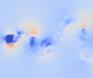
Figure 1. (a) Schematic of the wake problem geometry. (b) Instantaneous  $x_1$– $x_2$ snapshot of the dimensionless velocity magnitude for case (i).
For both DNS and LES, the dimensionless Navier–Stokes equations are solved in the incompressible limit using second-order centred differences on a staggered mesh (Harlow & Welch Reference Harlow and Welch1965), and the continuity condition is enforced using a fractional-step method (Kim & Moin Reference Kim and Moin1985). Two distinct solvers are used. The DNS and comparison-LES (i.e. non-DL) solver uses linearized-trapezoid time advancement in an alternating-direction implicit framework (Desjardins et al. Reference Desjardins, Blanquart, Balarac and Pitsch2008; MacArt & Mueller Reference MacArt and Mueller2016) and computes derivatives using non-uniformly weighted central differences. The DL-LES models are trained and evaluated using a standalone, Python-native solver with fourth-order Runge–Kutta time advancement and coordinate transforms calculated via statistical interpolation from the LES mesh (using the Scipy package's smooth spline approximation). In § 6, the trained DL-LES models are implemented in the DNS/comparison-LES solver, and the impact of its slightly ‘out-of-sample’ numerics is evaluated. The time step  $\Delta t$ is fixed with steady-state Courant–Friedrichs–Lewy numbers of approximately 0.4 for all cases.
The rectilinear mesh is non-uniform in  $x_1$– $x_2$ planes, with local refinement within the blockage boundary layers, and uniform in the $x_3$ direction. The refinement uses piecewise hyperbolic tangent functions in three regions (upstream, downstream and along the bluff body), with stretching factors $s_1=1.8$ along the bluff body and $s_2=1.1$ in the far-field regions. The $x_3$ mesh is uniform. The minimum DNS boundary layer mesh spacings, in wall units, are listed in table 1.
At the inflow boundary ( $-x_1$), Dirichlet conditions prescribe the uniform free stream velocity profile. The streamwise ( $\pm x_2$) boundaries are slip walls, and a convective outflow is imposed at the $+x_1$ boundary. The cross-stream ( $x_3$) direction is periodic.
Flow statistics are obtained by averaging in the cross-stream ( $x_3$) direction and time,
 \begin{equation} \langle \phi \rangle(x_1,x_2) = \frac{1}{L_3(t_f-t_s)}\int_{{-}L_3/2}^{L_3/2}\int_{t_s}^{t_f} \phi(x_1,x_2,x_3,t)\,{\rm d}t\,{\rm d}\,x_3, \end{equation}
where  $t_s$ and $t_f$ are the start and end times for averaging, respectively. The DNS calculations were advanced to steady state before recording statistics; the minimum time to steady state was $t_s=41.5$ dimensionless units (AR2 $\textit {Re}_0=2000$), and the maximum to steady state was $t_s=393$ units (AR1 $\textit {Re}_0=1000$). The minimum DNS recording window was $t_f-t_s=77$ time units (AR2 $\textit {Re}_0=1000$), and the maximum was $t_f-t_s=427$ time units (AR1 $\textit {Re}_0=1000$). The recording window for each case is listed in table 1. Spectra for the DNS lift coefficients have a minimum of two wavenumber decades below the shedding frequency for each case, indicating that the long-time vortex dynamics are sufficiently well represented in the statistics.
Instantaneous DNS fields  $u_i(x,t)$ were postprocessed to obtain filtered fields $\bar {u}_i(x,t)$,
 \begin{equation} \bar{u}_i(x,t) = \int_\varOmega G(x',x)u_i(x-x',t)\,{{\rm d}\,x}', \end{equation}
where  $G(x',x)$ is a box filter kernel with unit support within a ${\bar {\varDelta }}^3$ cube centred on $x$ (Clark, Ferziger & Reynolds Reference Clark, Ferziger and Reynolds1979). The DNS cases were filtered with local coarsening ratios ${\bar {\varDelta }}/\varDelta _{\rm{\small {DNS}}}=4$ (cases i, ii, iv) or 8 (case iii), where ${\bar {\varDelta }}$ is the local LES mesh spacing and $\varDelta _{\rm{\small {DNS}}}$ is the local DNS mesh spacing, such that a constant filtering ratio ${\bar {\varDelta }}/\varDelta _{\rm{\small {DNS}}}$ was maintained throughout the non-uniform computational mesh. One-sided filter kernels were applied near wall boundaries. All filtering was performed in the physical space. The resulting filtered fields were then downsampled by the same filter-to-DNS mesh ratios to obtain coarse-grained fields, representative of implicitly filtered LES solutions.
3.2. A posteriori LES
A posteriori LES calculations were initiated by restarting from filtered, downsampled DNS fields and were allowed to advance for several thousand time units before recording statistics. These calculations use grids coarsened by the same constant factors as the filtered, downsampled DNS fields, which is consistent with the common practice of implicitly filtered LES. The LES calculations therefore use  $1/64$ ( ${\bar {\varDelta }}/\varDelta _{\rm{\small {DNS}}}=4$) or $1/512$ ( ${\bar {\varDelta }}/\varDelta _{\rm{\small {DNS}}}=8$) the mesh points of the corresponding DNS calculations.
Comparison LES solutions were calculated for an implicit model (‘no-model LES’) and two eddy-viscosity models: the dynamic Smagorinsky (DS) model (Germano et al. Reference Germano, Piomelli, Moin and Cabot1991; Lilly Reference Lilly1992) and the anisotropic minimum dissipation (AMD) model (Rozema et al. Reference Rozema, Bae, Moin and Verstappen2015). Both model the SGS stress as
 \begin{equation} \tau^{\rm{\small{SGS}}}_{ij} ={-}2\nu_t \bar{S}_{ij} + \tfrac{1}{3}\tau^{\rm{\small{SGS}}}_{kk}\delta_{ij}, \end{equation}
where  $\nu _t$ is the eddy viscosity to be computed, $\bar {S}_{ij}=(\partial \bar {u}_i/\partial x_j + \partial \bar {u}_j/\partial x_i)/2$ is the filtered strain-rate tensor, and $\delta _{ij}$ is the Kronecker delta function. In incompressible solvers, the isotropic component is typically not modelled and is combined with the pressure-projection step. The Smagorinsky model (Smagorinsky Reference Smagorinsky1963) closes the SGS stress as
 \begin{equation} \tau^{\rm{\small{SGS}}}_{ij,\rm{\small DS}} \approx{-}2(C_S{\bar{\varDelta}})^2|\bar{S}|\bar{S}_{ij}, \end{equation}
where  $|\bar {S}|$ is the strain-rate magnitude, and the dynamic approach evaluates the coefficient $C_S$ using test filtering, least-squares solution and averaging across homogeneous directions. Our implementation uses the standard approach; for full details, the reader is referred to Germano et al. (Reference Germano, Piomelli, Moin and Cabot1991) and Lilly (Reference Lilly1992). The AMD model closes the SGS stress using (3.3) with the eddy viscosity evaluated as
 \begin{equation} \nu_{t,\rm{\small AMD}} = C_\rm{\small AMD} \frac{\max\left[-\left({\bar{\varDelta}}_k \dfrac{\partial \bar{u}_i}{\partial x_k}\right) \left( {\bar{\varDelta}}_k\dfrac{\partial \bar{u}_j}{\partial x_k}\right)\bar{S}_{ij}, 0\right]}{\dfrac{\partial \bar{u}_m}{\partial x_l}\dfrac{\partial \bar{u}_m}{\partial x_l}}, \end{equation}
where  ${\bar {\varDelta }}_k$ are the directional non-uniform mesh spacings and $C_{\rm{\small AMD}}=0.3$ for second-order central discretizations (Rozema et al. Reference Rozema, Bae, Moin and Verstappen2015). The AMD model is known to outperform the DS model on highly anisotropic meshes (Zahiri & Roohi Reference Zahiri and Roohi2019), as is the case here.
3.3. Deep learning model training and validation
Two DL-LES models are trained: one for case (i) and one for case (iii); these are denoted ‘DL-AR1’ and ‘DL-AR2’, respectively. Note that these training cases have different Reynolds numbers. Models are trained for a single configuration and tested in a posteriori LES on all configurations. The three out-of-sample configurations for each trained model have new physical characteristics (either AR or  $\textit {Re}_0$) for which the model has not been trained. The out-of-sample configurations are test/validation cases for the model. For example, one model is trained on data from case (iii) and then tested on cases (i), (ii), (iii) and (iv). Cases (i), (ii) and (iv) would then be completely out-of-sample. Case (iii) would be ‘quasi-out-of-sample’ in that the model has been trained on data from (iii) but only on short time intervals (see § 2.2) and is then simulated for (iii) over many flow times.
4. Mean-flow results
4.1. Drag coefficient
The predicted drag coefficients for the two DL-LES models and three comparison models, for each test case, are reported in table 2. Compared with the filtered DNS data, the deep learning models consistently perform as well or better than the dynamic Smagorinsky and AMD models. (No significant difference was observed between the DNS-evaluated and filtered-DNS-evaluated drag coefficients.) The AMD model is the most accurate of the non-DL models, though in all cases it is outperformed by the in-sample or nearest DL model. For example, for case (iv), the DL-AR2 model outperforms the DL-AR1 model, likely due to the higher degree of geometric similarity of the former to the AR4 bluff body. The implicitly modelled LES underperforms the learned models in all cases. The outperformance of DL-LES for predicting the drag coefficient is a direct consequence of its improved accuracy for modelling the mean velocity and Reynolds stress. Section 4.2 evaluates the DL-LES models’ accuracy for these statistics.
Table 2. Drag coefficients  $c_d$ evaluated from filtered DNS (f-DNS) and LES with different models: no-model (NM); dynamic Smagorinky (DS); anisotropic minimum dissipation (AMD); and deep learning (DL) models trained for cases (i) and (iii).

4.2. Mean-flow accuracy
The DNS- and LES-evaluated flow streamlines are shown in figures 2, 3, 4 and 5 for cases (i), (ii), (iii) and (iv). The LES-predicted streamlines are shown in colours; the no-model and dynamic Smagorinsky LES are combined on one plot.

Figure 2. AR1,  $Re_0=1000$ (i): streamlines of the mean flow field (DNS, black lines; LES, coloured lines). This case is in-sample for the DL-AR1 model. The flow is averaged across the centreline $y=0$.

Figure 3. AR2,  $Re_0=1000$ (ii): streamlines of the mean flow field (DNS, black lines; LES, coloured lines). This case is out-of-sample for all models. The flow is averaged across the centreline $y=0$.

Figure 4. AR2,  $Re_0=2000$ (iii): streamlines of the mean flow field (DNS, black lines; LES, coloured lines). This case is in-sample for the DL-AR2 model. The flow is averaged across the centreline $y=0$.

Figure 5. AR4,  $Re_0=1000$ (iv): streamlines of the mean flow field (DNS, black lines; LES: coloured lines). This case is out-of-sample for all models. The flow is averaged across the centreline $y=0$.
The DL-AR1 model is in-sample for the AR1,  $Re_0=1000$ case (figure 2), and produces the overall best a posteriori LES prediction. The implicitly modelled LES underpredicts the upper separation region and overpredicts the extent of the wake recirculation, while the opposite is true for the dynamic Smagorinsky- and AMD-modelled LES. The two DL models qualitatively match the DNS recirculation regions, with the DL-AR1 (in-sample) being visually more accurate.
For the AR2,  $Re_0=1000$ case (figure 3), the no-model and dynamic Smagorinsky LES both underpredict the extent of the upper separation region and overpredict that of the wake recirculation. The AMD model better predicts the upper separation but still overpredicts the wake recirculation. The DL-AR1 model is visually more accurate than the DL-AR2 model in this case despite its geometric similarity to the latter. This is likely due to the fact that the DL-AR1 model was trained for $Re_0=1000$, while the DL-AR2 model was trained for $Re_0=2000$. Both DL models are out-of-sample for this case, which highlights the DL models’ ability to generalize within small neighbourhoods of the training geometry and Reynolds number while remaining more accurate than the comparison models.
Increasing the Reynolds number in the AR2,  $Re_0=2000$ case (figure 4) significantly worsens the no-model prediction and slightly improves the dynamic Smagorinsky and AMD results. The DL-AR2 model, in-sample for this case, is more accurate than the DL-AR1 model (trained for the lower $Re_0=1000$) and each of the comparison models.
The AR4,  $Re_0=1000$ case (figure 5) is out-of-sample for both DL models, which both significantly outperform the no-model and dynamic Smagorinsky LES. In particular, the DL-AR1 model almost perfectly matches both recirculation regions. One would expect the DL-AR2 model to outperform the DL-AR1 model (due to the greater geometric similarity of the former to the AR4 test case), though the opposite is observed. One possibility is a greater influence of the Reynolds number on model accuracy than the blockage geometry. Both DL models are comparably accurate with the AMD model for this case, though the DL-AR2 model more accurately predicts the drag coefficient (table 2) than the AMD model.
Contour plots in figures 6 and 7 visualize the LES models’ domain accuracy for the AR2  $\textit {Re}_0=1000$ case (ii). At each mesh node, the LES-evaluated mean flow $\langle \bar {u}_i \rangle$, RMS velocity $\langle \bar {u}_i'' \rangle$ and shear component of the resolved Reynolds stress $\tau ^R_{ij}\equiv \langle \bar {u}_i\bar {u}_j \rangle - \langle \bar {u}_i \rangle \langle \bar {u}_j \rangle$ are compared with the corresponding filtered-DNS fields using the $\ell _1$ error
 \begin{equation} \ell_{1,\phi} = \left|\langle {\phi}^{\rm{\small{LES}}} \rangle - \langle {\phi}^{\rm{\small{DNS}}} \rangle\right| \end{equation}
for a flow statistic  $\phi$. Compared with the benchmark LES models, the DL-LES models consistently reduce the prediction error for the mean-flow and RMS statistics. The DL-LES models achieve particular accuracy improvements near the walls of the rectangular prism; this leads directly to higher accuracy in computing the drag coefficient.

Figure 6. The  $\ell _1$ error for the streamwise and cross-stream mean velocity components (a,b) and the shear component of the resolved Reynolds stress (c) for the AR2 $\textit {Re}_0=1000$ configuration (ii).

Figure 7. The  $\ell _1$ error for the resolved velocity fluctuations for the AR2 $\textit {Re}_0=1000$ configuration (ii).
Figures 8 and 9 show scatter plots of the LES-predicted fields versus the filtered DNS fields for cases (i) and (iv), respectively. The scatter plots provide a compact representation of the accuracy of the LES calculations across the simulation domain. The  $1:1$ line represents predictions with $100\,\%$ accuracy relative to the filtered-DNS fields. The DL-LES models consistently outperform the benchmark LES models, and in several cases, the DL-LES models dramatically improve the predictive accuracy.

Figure 8. AR1  $\textit {Re}_0=1000$ (i): comparison of averaged a posteriori LES fields with a priori filtered DNS fields for (a) $\langle \bar {u}_1\rangle$, (b) $\langle \bar {u}_2\rangle$, (c) $\tau ^R_{12}$, (d) $\tau ^R_{11}$, (e) $\tau ^R_{22}$ and ( f) $\tau ^R_{33}$ (black lines indicate $1:1$).

Figure 9. AR4  $\textit {Re}_0=1000$ (iv): comparison of averaged a posteriori LES fields with a priori filtered DNS fields for (a) $\langle \bar {u}_1\rangle$, (b) $\langle \bar {u}_2\rangle$, (c) $\tau ^R_{12}$, (d) $\tau ^R_{11}$, (e) $\tau ^R_{22}$, and ( f) $\tau ^R_{33}$ (black lines indicate $1:1$).
Regions of severely outlying points are visible in the resolved Reynolds for the no-model and dynamic Smagorinsky LES. These points are confined to the boundary-layer regions, where the filtered-DNS statistics approach zero but the no-model and dynamic Smagorinsky LES are incorrectly large. The AMD model improves the near-wall predictions, though it still exhibits larger variance about the  $1:1$ line for $\tau ^R_{11}$ and $\tau ^R_{22}$ than the DL-LES models. For all cases and all statistics, the DL-LES results more closely match the filtered-DNS-evaluated statistics than the no-model, dynamic Smagorinsky and AMD LES.
4.3. Near-wall accuracy
Comparing the DNS- and LES-predicted flow fields close to the bluff-body walls is instructive to understand the performance of the trained DL-LES models within boundary-layer regions. With the mean shear stress at the wall computed as  $\tau _{12}(x_1,\pm H_0/2)=\rho \nu (\partial \langle \bar {u}_1 \rangle (x_1,\pm H_0/2)/\partial x_2)$, the wall shear stress is $\tau _w(x_1) = (\tau _{12}(x_1,H_0/2) - \tau _{12}(x_1,-H_0/2))/2$, the friction velocity is $u_\tau =\sqrt {\tau _w/\rho }$, and the viscous length scale is $\delta _v=\nu /u_\tau$. The flow near the wall is presented in wall units, $y^+=x_2/\delta _v$, and the corresponding normalized, averaged, filtered velocity components are $\langle \bar {u}_i \rangle ^+=\langle \bar {u}_i \rangle /u_\tau$.
Figure 10 plots the DNS- and LES-evaluated mean streamwise and cross-stream velocity components in wall units. In the figures, the velocity components are offset on the abscissas to show several streamwise locations, and all data are averaged about the domain centreline, accounting for the sign change in the mean cross-stream velocity. The LES and DNS data are reported on the respective coarse LES and fine DNS meshes, which illustrates the reduction in near-wall resolution inherent to the testing LES cases: for most cases and streamwise locations, the LES mesh does not resolve within  $y^+=10$. Wall models were not employed in any of the LES calculations.

Figure 10. Near-wall streamwise (a,c,e,g) and cross-stream (b,d, f,h) mean velocity profiles in wall units. Vertical dashed lines indicate  $x_1$ locations. Reference DNS data are plotted on the fine DNS meshes. All lines start at the first mesh node away from the wall.
For most cases, the DL-LES models generally slightly outperform the AMD model and dramatically outperform the dynamic Smagorinsky model and implicitly modelled LES. For the AR1,  $\textit {Re}_0=1000$ cross-stream velocity, only the in-sample trained DL-AR1 model captures the sign reversal near $x_1=0$, which directly affects the shape of the predicted separation bubble (figure 2). For AR2, $\textit {Re}_0=2000$ case, the in-sample DL-AR2 model likewise best predicts the cross-stream velocity field at all streamwise locations, and the AMD model is not more accurate than the dynamic Smagorinsky and implicitly modelled LES. The DL-LES models are also robust to every out-of-sample case, for which they outperform the dynamic Smagorinsky and implicitly modelled LES and are competitive to the in-sample DL-LES models.
5. Adjoint-based optimization versus a priori optimization
We also numerically compare our adjoint-optimization approach with a priori optimization. The latter has been widely used in fluid dynamics. A priori optimization does not optimize over the LES equations but instead calibrates neural-network parameters offline: it uses standard supervised-learning methods to predict the DNS-evaluated SGS stress (Reynolds stress) using the a priori filtered (averaged) DNS velocities as model inputs. The objective function for a priori training is therefore decoupled from the RANS/LES PDE model, which can reduce predictive accuracy and even cause instability in a posteriori predictions (i.e. substituting the trained closure model into a LES or RANS calculation) (Sirignano et al. Reference Sirignano, MacArt and Freund2020; MacArt et al. Reference MacArt, Sirignano and Freund2021). A priori optimization does not optimize over the predictive model (the LES equations) but instead over a different objective function that might not be well aligned with the true objective function (the predictive accuracy of the LES equations). For example, an a priori-trained neural network will receive DNS variables as inputs during optimization but will receive LES/RANS variables during simulations.
Instead, the adjoint-based approach optimizes over the a posteriori LES calculation, which is the ‘true’ predictive model, in the sense that the overall predictive accuracy of LES (not merely the SGS stress) is desired. Unlike a priori optimization, the objective function for the adjoint-based approach is entirely consistent with the predictive model. In practice, the adjoint-based approach has been consistently found to outperform offline training in numerical simulations (Sirignano et al. Reference Sirignano, MacArt and Freund2020; MacArt et al. Reference MacArt, Sirignano and Freund2021). The present numerical comparison between the two optimization approaches reaches a similar conclusion.
We train a neural network closure model using a priori optimization on the filtered DNS data for the AR1  $\textit {Re}_0=1000$ case. The a priori-trained closure model has identical architecture and hyperparameters as the neural network used for adjoint-trained DL-LES models (§ 2.1). Figure 11 illustrates the accuracy of the a priori-trained model outputs versus the ‘exact’, DNS-evaluated SGS stress components. The modelled SGS stress aligns almost perfectly with the DNS SGS stress, indicating that the a priori model has been sufficiently trained. It should be noted that figure 11 displays the output of the closure model evaluated on the filtered DNS (i.e. it shows a priori results). As we demonstrate subsequently, the a priori-trained closure model produces less-accurate a posteriori predictions than the adjoint-trained DL-LES model.

Figure 11. A priori-learned  $\tau _{ij}^{\rm{\small {SGS}}}$ (AR1 $\textit {Re}_0=1000$) compared with the target DNS values used for training. Values are averaged over the spanwise ( $x_3$) direction and time.
Once trained, the a priori-neural network closure model is substituted into the LES equations and simulated a posteriori. Figure 12 compares the a posteriori LES mean flow and variance terms using the two models for the AR1  $\textit {Re}_0=1000$ configuration (in-sample only). For all flow statistics, the adjoint-trained DL-LES model – which has been trained by optimizing over the entire LES equations – substantially outperforms the a priori-trained model, even for this in-sample test.

Figure 12. Comparison of a priori DL to adjoint-based DL:  $\ell _1$ error of the streamwise and cross-stream mean velocity components, shear component of the resolved Reynolds stress, and resolved velocity fluctuations. Shown for the AR1 $\textit {Re}_0=1000$ configuration (i).
6. Out-of-sample geometries
While the slight geometric differences considered in §§ 3 and 4 are useful for comparing LES models’ relative performance, true utility requires trained models to maintain accuracy (generalize) to significantly different geometries. The models trained for rectangular prisms are now tested for two completely out-of-sample geometries: an equilateral triangular prism and a cylinder, both for bulk Reynolds number  $Re_0=1000$ and characteristic height (diameter) $H_0=1$. All a posteriori LES calculations for these geometries – including the DL-LES predictions – use the DNS/comparison-LES flow solver, which has overall similar numerical methods to the DL-LES model-training solver but (a) uses semi-implicit time advancement and (b) does not use the same coordinate transformation-based discretization. The triangle and cylinder tests therefore pose the additional challenge of evaluating the trained DL-LES models in an out-of-sample numerical solver.
Streamlines for LES using the trained models and comparison models are shown for the triangular prism in figure 13 and the cylinder in figure 14. For the triangular prism, the AMD model is least accurate, the DL-AR1 model is comparably accurate with the no-model and dynamic-Smagorinsky LES, and the DL-AR2 model is highly accurate, nearly matching the DNS streamlines. For the cylinder, the DL-AR1 and DL-AR2 models both suppress all artificial primary recirculation, which is correct compared with the DNS, while the implicitly modelled LES and AMD model incorrectly predict two recirculation regions. The extent of the separation bubble is also more correctly predicted by the DL-LES models than any of the comparison models.

Figure 13. Equilateral triangular prism,  $Re_0=1000$: streamlines of the average flow field (DNS, black lines; LES, coloured lines). This case is out-of-sample for all models.

Figure 14. Cylinder,  $Re_0=1000$: streamlines of the average flow field (DNS, black lines; LES, coloured lines). This case is out-of-sample for all models.
Figure 15 compares a posteriori LES results of the two flow solvers (the DL-LES model-training solver versus the DNS/comparison-LES solver) for the AR2,  $Re_0=1000$ rectangular prism using the AR2, $Re_0=2000$-trained DL-LES model, which is out-of-sample for this case. The two LES solvers produce similar predictions in the primary separation region, matching the DNS. In the wake region, the comparison-LES solver is less accurate than the model-training solver, as could be anticipated due to its numerical differences, though the accuracy difference is smaller than that between the DL-LES and comparison-LES models (figures 3, 6 and 7).

Figure 15. Comparison of a posteriori LES calculations for the AR2,  $Re_0=1000$ case computed using (a) the model-training flow solver (DL-AR2) and (b) the DNS/comparison-LES flow solver (NGA-DL-AR2). Both use the AR2, $Re_0=2000$-trained DL-LES model. The DNS solution is shown in black lines.
A major concern in using deep learning for computational physics is that trained models will not generalize well to out-of-sample geometries. This result is therefore significant, for it gives hope that adjoint-trained models for realistic aerodynamic geometries could be successfully applied to substantially different geometries. A further concern with adjoint-based optimization in particular that the method will overfit, in a sense, to the numerical methods used for training. The fact that the trained DL-LES models are at least stable, and in some cases accurate, indicates a robustness to out-of-sample numerical methods. Of course, this generalizability can be expected to degrade for far out-of-sample methods (e.g. finite elements instead of finite differences), though this remains to be tested.
7. Conclusion
Fully resolved calculations of wall-bounded flows can be computationally prohibitive due to the extremely small mesh sizes needed to adequately resolve boundary-layer turbulence. A deep learning closure model for LES of wall-bounded flows was developed and demonstrated for turbulent flows around rectangular prisms of different aspect ratios and Reynolds numbers, as well as out-of-sample equilateral triangular prism and cylinder geometries.
Two DL-LES models were trained using adjoint-based, PDE-constrained optimization methods. These optimize over the entire PDE solution to select the closure-model parameters, which ensures consistency of the closure model with the PDE. The current work used deep neural networks, though in practice any multiparametric closure model (including, for example, traditional one- or two-equation closures) could be substituted.
In a posteriori predictions, the DL-LES models were significantly more accurate than the commonly used dynamic Smagorinsky model, and implicitly modelled LES, yielding better predictions for the drag coefficient, mean velocity, RMS velocity, resolved Reynolds stress for Reynolds numbers and prism aspect ratios not seen in training. Compared with the recent AMD model, the DL-LES models are generally more accurate for mean-flow predictions, including near bluff-body walls, even for out-of-sample aspect ratios and geometries, though the DL-LES and AMD models had similar error for the RMS velocity components.
Our results indicate that deep learning closure models have the potential to improve the accuracy of LES calculations for out-of-sample aerodynamic shapes, particularly when optimization is done over the flow PDEs, which results in long-time stable predictive calculations that are not necessarily guaranteed by a priori optimization.
Another challenge that should be addressed in future research is to increase the symmetry of DL-LES simulations, for example, by leveraging tensor basis neural networks (TBNNs) and rotationally invariant model inputs. Model generalization to more complex flow geometries, including airfoils at stall conditions, is being pursued.
Our training method (adjoint equations and gradient descent) could also be used to train an LES closure model for an unstructured-mesh simulation. The optimization method in § 2 is presented for a Cartesian mesh with coordinate transforms, though in principle any semidiscretization – including unstructured finite-volume or finite-element discretizations – could be used without fundamental changes to the algorithm.
Finally, it should be noted that only low Reynolds numbers were used for training and testing. Extensions to flight-relevant Reynolds numbers will be crucial, though they will come of course at high computational expense. We note that preliminary tests of the present  $\textit {Re}_0=1000$ and $\textit {Re}_0=2000$-trained models to a $\textit {Re}_0=12\,000$ wake flow are stable and, in some cases, accurate, though a full exploration of this and extensions to high-Reynolds-number experimental data are left for future work.
Funding
This material is based in part upon work supported by the US National Science Foundation under award CBET-22-15472. This research used resources of the Oak Ridge Leadership Computing Facility, which is a DOE Office of Science User Facility supported under contract DE-AC05-00OR22725. The authors acknowledge computational time on resources supported by the University of Notre Dame Center for Research Computing (CRC).
Declaration of interests
The authors report no conflict of interest.


 Open access