


1. Introduction
The interest in gravity currents within porous media is motivated by the need to model environmental and industrial processes in which an intruding fluid propagates inside a porous medium saturated with another fluid (Ungarish Reference Ungarish2009).
The spreading of these currents is governed by the interplay between the pressure/buoyancy forces during the flow and the resistive viscous forces. Semi-analytical models for such currents are available to describe their propagation in porous domains of infinite extent having plane (Huppert & Woods Reference Huppert and Woods1995) or radial geometry (Lyle et al. Reference Lyle, Huppert, Hallworth, Bickle and Chadwick2005), under instantaneous or continuous mass injection at the domain origin. A prototype case concerns the spreading of groundwater or liquid waste mound, injected instantaneously in a homogeneous medium of infinite extent, which illustrates the response of the system to a pulse input. An analytical solution to this problem was derived for a constant mound volume by Barenblatt (Reference Barenblatt1952) in self-similar form. In some cases, the mound volume is not conserved due to a loss of fluid; this is typically the case of the response of a porous bank to a sudden surge of water level in an adjacent channel, which rapidly reverts to its original value. As a consequence, the water mound infiltrating the porous bank partially drains back into the channel. Here, while the total mass present within the porous domain decreases over time, the first spatial moment of the mound (also termed the dipole moment of the flow) is conserved, as first shown in the seminal work of Barenblatt & Zel’dovich (Reference Barenblatt and Zel’dovich1957). These authors derived a self-similar solution describing the spreading of the mound in the intermediate asymptotic regime, i.e. at time scales much larger than the duration of the surge initiating the motion, yet smaller than needed to reach the final equilibrium condition, or the outer boundary of the system (see figure 1). This dipole solution has been extended to several dimensions by Hulshof & Vazquez (Reference Hulshof and Vazquez1993). Wagner (Reference Wagner2005) discussed a similarity solution of the second kind of the dipole problem including capillarity. Barenblatt & Vazquez (Reference Barenblatt and Vazquez1998) extended the dipole solution to the case of an assigned outgoing flux at a moving boundary. King & Woods (Reference King and Woods2003) verified the classical dipole solution performing experiments using a Hele-Shaw cell, obtaining a good agreement with the theoretical results; they then extended the model and experiments to include drainage effects. Mathunjwa & Hogg (Reference Mathunjwa and Hogg2007) incorporated a vertical permeability variation in the dipole solution and showed it to be linearly stable.

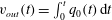
Figure 1. Diagram showing a mound of fluid of density
 ${\it\rho}$
and height
${\it\rho}$
and height
 $h(x,t)$
spreading over an impermeable base in a porous medium saturated with fluid of density
$h(x,t)$
spreading over an impermeable base in a porous medium saturated with fluid of density
 ${\it\rho}-{\rm\Delta}{\it\rho}$
and draining freely at
${\it\rho}-{\rm\Delta}{\it\rho}$
and draining freely at
 $x=0$
. Porosity and permeability vary with elevation
$x=0$
. Porosity and permeability vary with elevation
 $z$
as
$z$
as
 ${\it\phi}={\it\phi}_{0}(z/x^{\ast })^{{\it\gamma}-1}$
and
${\it\phi}={\it\phi}_{0}(z/x^{\ast })^{{\it\gamma}-1}$
and
 $k=k_{0}(z/x^{\ast })^{{\it\omega}-1}$
. The diagrams for
$k=k_{0}(z/x^{\ast })^{{\it\omega}-1}$
. The diagrams for
 ${\it\phi}$
and
${\it\phi}$
and
 $k$
refer to
$k$
refer to
 ${\it\gamma}=2$
and
${\it\gamma}=2$
and
 ${\it\omega}=4$
, respectively, coincident to the values adopted in our experiments.
${\it\omega}=4$
, respectively, coincident to the values adopted in our experiments.
The body of knowledge accumulated on gravity driven flows in porous media concerns mainly water and other Newtonian liquids. However, fluids flowing in natural and artificial porous media in a variety of environmental and industrial contexts often display a complex rheological nature. Relevant applications include, but are not limited to, environmental contamination and in situ remediation, enhanced oil recovery operations, filtration of polymer solutions and slurries, textiles and paper manufacturing, food processing, biological systems and biomedical techniques (e.g., Vossoughi Reference Vossoughi1999; Ciriello & Di Federico Reference Ciriello and Di Federico2012, and references therein).
The nature of the nonlinear relationship between stress and shear rate also varies greatly, and fluids of interest are grouped into three classes: (i) time-independent, (ii) time-dependent and (iii) viscoelastic. Time-independent models are the most widely used for flow problems in porous media (Wu & Pruess Reference Wu and Pruess1996). Among these, the power-law, or the Ostwald-de Waele model, is a two parameter simplification of more complex relationships. It approximately describes the behaviour of time-independent non-Newtonian fluids over an intermediate range of shear rates and in the absence of yield stress and has been successfully adopted to describe the flow of polymer solutions, foams and crude oils in porous media. Environmental contaminants such as slurries or dredged fluid mud (Yilmaz, Testik & Chowdury Reference Yilmaz, Testik and Chowdury2014) and carriers for remediation agents (Tosco et al. Reference Tosco, Papini, Viggi and Sethi2014) are usually represented either via the power-law model, or using more complex constitutive equations including a yield stress; even in the latter case however, the adoption of a pure power-law model (approximating the Herschel–Bulkley constitutive equation for vanishing values of the yield stress) permits mathematical predictions that are upper bounds for the exact solution, or may work as benchmarks for numerical codes.
The modelling of gravity currents of non-Newtonian fluids is of importance whenever density differences act as the main driving force in porous media flow of rheologically complex fluids. Most literature studies addressing non-Newtonian gravity currents in porous media adopt a power-law rheological model. The propagation of such currents was analysed by Pascal & Pascal (Reference Pascal and Pascal1993) for constant injected volume and plane geometry, and by Bataller (Reference Bataller2008) for assigned depth or flux at the origin and radial geometry. General solutions for a time-variable current volume were derived in a two-dimensional (Di Federico, Archetti & Longo Reference Di Federico, Archetti and Longo2012a ) and axisymmetric geometry (Di Federico, Archetti & Longo Reference Di Federico, Archetti and Longo2012b ); the results obtained in the latter paper were confirmed by the experiments of Longo et al. (Reference Longo, Di Federico, Chiapponi and Archetti2013b ).
To the best of our knowledge, the classical dipole problem (discussed above for a Newtonian fluid) was never formulated or solved for the non-Newtonian case. This model mimics the instantaneous release of a fluid with complex rheological behaviour in a semi-infinite porous medium due to a sudden surge in level at the boundary. As such, it represents for example the spreading of industrial effluents or slurries produced by mining activities, which are typically conveyed to disposal or tailings areas by means of open channels or flumes (Burger, Haldenwang & Alderman Reference Burger, Haldenwang and Alderman2015). An overflow in the channel causes the transported material to go over the channel walls and spread into the adjoining porous bank. Another relevant scenario is the free-surface advancement of remediation agents such as nanoscale zerovalent iron (Tosco et al. Reference Tosco, Papini, Viggi and Sethi2014) dispersed in aqueous slurries in aquifer systems. In both cases, the size and shape of subsurface domain invaded by the spreading needs to be assessed.
In this paper, we derive a solution to the dipole problem for a non-Newtonian power-law fluid in a porous medium, including the effect of spatial heterogeneity. The well-known tendency of natural media to display variations in permeability is conceptualized with a continuous power-law variation along the vertical direction, mimicking the sub-horizontal stratifications of porous media, or the change in fracture density with depth for densely fractured media. A vertical porosity gradient is added to the conceptual model, taking into account that in real media, variations in permeability and porosity are often interdependent (Phillips Reference Phillips1991; Dullien Reference Dullien1992). The presence of permeability and porosity gradients parallel or perpendicular to the flow direction has been shown to affect significantly the shape of gravity currents of Newtonian (Huppert & Woods Reference Huppert and Woods1995; Zheng et al. Reference Zheng, Soh, Huppert and Stone2013) or non-Newtonian (Di Federico et al. Reference Di Federico, Longo, Chiapponi, Archetti and Ciriello2014) fluids within porous domains.
A closed form solution to this problem is obtained in similarity form for shear-thinning fluids, extending the work of King & Woods (Reference King and Woods2003), who treated the dipole flow for a Newtonian fluid and vertically variable permeability. In variance with their results, the first spatial moment is conserved only for a specific class of self-similar solutions, and the height of the fluid mound in the origin is non-zero and finite. We then explore the conditions for the validity of a Hele-Shaw analogue model, and present results from a set of laboratory experiments which test the constancy of the dipole moment, and the similarity solution obtained. In both cases, a good agreement is obtained between theoretical and experimental results.
2. Formulation
We study the gravity-driven flow of a viscous non-Newtonian fluid having density
 ${\it\rho}$
and spreading along the horizontal impermeable base of an infinite homogeneous porous domain of depth
${\it\rho}$
and spreading along the horizontal impermeable base of an infinite homogeneous porous domain of depth
 $h_{0}$
, initially saturated with an ambient fluid of density
$h_{0}$
, initially saturated with an ambient fluid of density
 ${\it\rho}-{\rm\Delta}{\it\rho}$
. The intruding fluid is described rheologically by a power-law model, which uses two parameters, flow behaviour index
${\it\rho}-{\rm\Delta}{\it\rho}$
. The intruding fluid is described rheologically by a power-law model, which uses two parameters, flow behaviour index
 $n$
and consistency index
$n$
and consistency index
 $\widetilde{{\it\mu}}$
, to express the shear stress
$\widetilde{{\it\mu}}$
, to express the shear stress
 ${\it\tau}$
as a function of shear rate
${\it\tau}$
as a function of shear rate
 $\dot{{\it\gamma}}$
in the form
$\dot{{\it\gamma}}$
in the form
 ${\it\tau}=\widetilde{{\it\mu}}|\dot{{\it\gamma}}|^{n-1}\dot{{\it\gamma}}$
, valid for simple shear. The cases
${\it\tau}=\widetilde{{\it\mu}}|\dot{{\it\gamma}}|^{n-1}\dot{{\it\gamma}}$
, valid for simple shear. The cases
 $n<1$
,
$n<1$
,
 $n=1$
, and
$n=1$
, and
 $n>1$
correspond to shear-thinning, Newtonian, and shear-thickening behaviour, respectively. For
$n>1$
correspond to shear-thinning, Newtonian, and shear-thickening behaviour, respectively. For
 $n=1$
, the consistency index
$n=1$
, the consistency index
 $\widetilde{{\it\mu}}$
becomes the dynamic viscosity
$\widetilde{{\it\mu}}$
becomes the dynamic viscosity
 ${\it\mu}$
.
${\it\mu}$
.
A finite mound of fluid is released in the half-plane
 $x>0$
and can drain freely at
$x>0$
and can drain freely at
 $x=0$
, see figure 1. The space–time development of the current height
$x=0$
, see figure 1. The space–time development of the current height
 $h(x,t)$
is determined under the assumption of a thin gravity current having a large ratio between horizontal and vertical length scales (Bear Reference Bear1972), and small height with respect to the thickness of the porous domain (
$h(x,t)$
is determined under the assumption of a thin gravity current having a large ratio between horizontal and vertical length scales (Bear Reference Bear1972), and small height with respect to the thickness of the porous domain (
 $h(x,t)\ll h_{0}$
). This allows modelling of the propagation as one-dimensional (neglecting vertical velocities) and the motion of the displaced fluid may be disregarded. The pressure within the intruding fluid is hydrostatic and given by
$h(x,t)\ll h_{0}$
). This allows modelling of the propagation as one-dimensional (neglecting vertical velocities) and the motion of the displaced fluid may be disregarded. The pressure within the intruding fluid is hydrostatic and given by
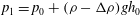
 $$\begin{eqnarray}p(x,z,t)=p_{1}+{\rm\Delta}{\it\rho}gh(x,t)-{\it\rho}gz,\end{eqnarray}$$
where
 $p_{1}=p_{0}+({\it\rho}-{\rm\Delta}{\it\rho})gh_{0}$
is a constant, and
$p_{1}=p_{0}+({\it\rho}-{\rm\Delta}{\it\rho})gh_{0}$
is a constant, and
 $p_{0}$
is the constant pressure at
$p_{0}$
is the constant pressure at
 $z=h_{0}$
. The sharp interface approximation is assumed to hold; we neglect mixing due to convection assuming that no interface instabilities develop, and mixing by molecular diffusion assuming that the time scale of molecular diffusion is much longer than the time scale of the process. Surface tension effects are also neglected; this may be a limitation for very low-permeability media, as it implies disregarding of the capillary entry pressure limiting the migration of the injected fluid. We further assume the validity of the modified Darcy’s equation for power-law fluid flow in porous media (Pascal Reference Pascal1983; Shenoy Reference Shenoy1995)
$z=h_{0}$
. The sharp interface approximation is assumed to hold; we neglect mixing due to convection assuming that no interface instabilities develop, and mixing by molecular diffusion assuming that the time scale of molecular diffusion is much longer than the time scale of the process. Surface tension effects are also neglected; this may be a limitation for very low-permeability media, as it implies disregarding of the capillary entry pressure limiting the migration of the injected fluid. We further assume the validity of the modified Darcy’s equation for power-law fluid flow in porous media (Pascal Reference Pascal1983; Shenoy Reference Shenoy1995)
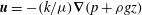
 $$\begin{eqnarray}\displaystyle \displaystyle \boldsymbol{u}=-{\it\Lambda}_{0}^{1/n}{\it\phi}^{(n-1)/2n}k^{(n+1)/2n}|\boldsymbol{{\rm\nabla}}(p+{\it\rho}gz)|^{(1/n-1)}\boldsymbol{{\rm\nabla}}(p+{\it\rho}gz), & & \displaystyle\end{eqnarray}$$
 $$\begin{eqnarray}\displaystyle \displaystyle {\it\Lambda}_{0}(\widetilde{{\it\mu}},n)=\frac{1}{2\widetilde{{\it\mu}}C_{t}}\left(\frac{50}{3}\right)^{(n+1)/2}\left(\frac{n}{3n+1}\right)^{n}, & & \displaystyle\end{eqnarray}$$
where
 $\boldsymbol{u}$
is the Darcy velocity,
$\boldsymbol{u}$
is the Darcy velocity,
 $p$
the pressure in the intruding fluid,
$p$
the pressure in the intruding fluid,
 $g$
the gravity,
$g$
the gravity,
 $z$
the vertical coordinate and
$z$
the vertical coordinate and
 ${\it\phi}$
and
${\it\phi}$
and
 $k$
are the medium porosity and intrinsic permeability, respectively. Equation (2.2) derives from the capillary bundle analogy for power-law fluid flow, modified to take tortuosity effects into account via a factor
$k$
are the medium porosity and intrinsic permeability, respectively. Equation (2.2) derives from the capillary bundle analogy for power-law fluid flow, modified to take tortuosity effects into account via a factor
 $C_{t}>1$
, which has several possible expressions (for a review, see Shenoy Reference Shenoy1995). The expression implemented here in (2.3) (for the details, see Di Federico et al.
Reference Di Federico, Archetti and Longo2012a
), is
$C_{t}>1$
, which has several possible expressions (for a review, see Shenoy Reference Shenoy1995). The expression implemented here in (2.3) (for the details, see Di Federico et al.
Reference Di Federico, Archetti and Longo2012a
), is
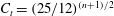 $C_{t}=(25/12)^{(n+1)/2}$
(Pascal Reference Pascal1983). As a whole, the prefactor on the left-hand side of (2.2) is akin to an effective fluid mobility, and depends on medium properties (porosity/permeability) in a nonlinear fashion based on the value of the flow behaviour index
$C_{t}=(25/12)^{(n+1)/2}$
(Pascal Reference Pascal1983). As a whole, the prefactor on the left-hand side of (2.2) is akin to an effective fluid mobility, and depends on medium properties (porosity/permeability) in a nonlinear fashion based on the value of the flow behaviour index
 $n$
. For a Newtonian fluid,
$n$
. For a Newtonian fluid,
 $C_{t}=(25/12)$
(Cristopher & Middleman Reference Cristopher and Middleman1965), the factor
$C_{t}=(25/12)$
(Cristopher & Middleman Reference Cristopher and Middleman1965), the factor
 ${\it\Lambda}_{0}$
in (2.3) reduces to
${\it\Lambda}_{0}$
in (2.3) reduces to
 $1/{\it\mu}$
and (2.2) to Darcy’s law
$1/{\it\mu}$
and (2.2) to Darcy’s law
 $\boldsymbol{u}=-(k/{\it\mu})\boldsymbol{{\rm\nabla}}(p+{\it\rho}gz)$
.
$\boldsymbol{u}=-(k/{\it\mu})\boldsymbol{{\rm\nabla}}(p+{\it\rho}gz)$
.
The permeability and porosity of the medium are assumed to vary along the vertical as
 $$\begin{eqnarray}k=k_{0}\left({\displaystyle \frac{z}{x^{\ast }}}\right)^{{\it\omega}-1},\quad {\it\phi}={\it\phi}_{0}\left({\displaystyle \frac{z}{x^{\ast }}}\right)^{{\it\gamma}-1},\end{eqnarray}$$
where
 $x^{\ast }$
is a reference length scale,
$x^{\ast }$
is a reference length scale,
 $k_{0}$
and
$k_{0}$
and
 ${\it\phi}_{0}$
are the permeability and porosity at
${\it\phi}_{0}$
are the permeability and porosity at
 $z=x^{\ast }$
, respectively, and
$z=x^{\ast }$
, respectively, and
 ${\it\omega}$
and
${\it\omega}$
and
 ${\it\gamma}$
are constant numerical coefficients.
${\it\gamma}$
are constant numerical coefficients.
 ${\it\omega}>1~({\it\gamma}>1)$
or
${\it\omega}>1~({\it\gamma}>1)$
or
 ${\it\omega}<1~({\it\gamma}<1)$
represent a permeability (porosity) increasing or decreasing with
${\it\omega}<1~({\it\gamma}<1)$
represent a permeability (porosity) increasing or decreasing with
 $z$
, respectively. We further set
$z$
, respectively. We further set
 ${\it\gamma}>{\it\gamma}_{1}=0$
and
${\it\gamma}>{\it\gamma}_{1}=0$
and
 ${\it\omega}>{\it\omega}_{1}={\it\gamma}(1-n)/(n+1)$
; this ensures the validity of the velocity scale defined in the following. The lower bounds
${\it\omega}>{\it\omega}_{1}={\it\gamma}(1-n)/(n+1)$
; this ensures the validity of the velocity scale defined in the following. The lower bounds
 ${\it\gamma}_{1}$
and
${\it\gamma}_{1}$
and
 ${\it\omega}_{1}$
imply that porosity and permeability do not decrease faster than
${\it\omega}_{1}$
imply that porosity and permeability do not decrease faster than
 $z^{-1}$
with elevation. This constraint is of limited impact as in most real applications to porous and fractured media, the permeability tends to decrease with depth (Jiang, Wang & Wan Reference Jiang, Wang and Wan2010), hence the case
$z^{-1}$
with elevation. This constraint is of limited impact as in most real applications to porous and fractured media, the permeability tends to decrease with depth (Jiang, Wang & Wan Reference Jiang, Wang and Wan2010), hence the case
 ${\it\omega}>1$
is more common than
${\it\omega}>1$
is more common than
 ${\it\omega}<1$
.
${\it\omega}<1$
.
Note that in real porous media, the two exponents
 ${\it\omega}-1$
and
${\it\omega}-1$
and
 ${\it\gamma}-1$
are related, and their ratio typically varies between
${\it\gamma}-1$
are related, and their ratio typically varies between
 $2$
and
$2$
and
 $3$
(Phillips Reference Phillips1991; Dullien Reference Dullien1992), corresponding to two limiting cases of the mediums microstructure, i.e. media with tubular fluid paths and with an intersecting network of cracks or fissures, respectively.
$3$
(Phillips Reference Phillips1991; Dullien Reference Dullien1992), corresponding to two limiting cases of the mediums microstructure, i.e. media with tubular fluid paths and with an intersecting network of cracks or fissures, respectively.
For a mound of Newtonian fluid propagating in a semi-infinite homogeneous medium and draining at the origin, the volume decreases in time, but the first spatial moment
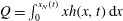 $Q=\int _{0}^{x_{N}(t)}xh(x,t)\,\text{d}x$
, with
$Q=\int _{0}^{x_{N}(t)}xh(x,t)\,\text{d}x$
, with
 $x_{N}$
the position of the current front, is time invariant. The constancy of
$x_{N}$
the position of the current front, is time invariant. The constancy of
 $Q$
, also termed the dipole moment, was first shown by Barenblatt & Zel’dovich (Reference Barenblatt and Zel’dovich1957). The large-time behaviour of the solution is well represented by self-similar functions, which have been demonstrated to converge to the general solution of the dipole problem (see Barenblatt & Vazquez Reference Barenblatt and Vazquez1998). In the following, we generalize the solution of the dipole problem (King & Woods Reference King and Woods2003) to non-Newtonian power-law fluids and vertically variable permeability and porosity, described by (2.4a,b
).
$Q$
, also termed the dipole moment, was first shown by Barenblatt & Zel’dovich (Reference Barenblatt and Zel’dovich1957). The large-time behaviour of the solution is well represented by self-similar functions, which have been demonstrated to converge to the general solution of the dipole problem (see Barenblatt & Vazquez Reference Barenblatt and Vazquez1998). In the following, we generalize the solution of the dipole problem (King & Woods Reference King and Woods2003) to non-Newtonian power-law fluids and vertically variable permeability and porosity, described by (2.4a,b
).
Under the previous assumptions, the flow equation (2.2) simplifies to its one-dimensional version, which reads in terms of the horizontal velocity
 $u(x,z,t)$
as
$u(x,z,t)$
as
 $$\begin{eqnarray}\displaystyle u(x,z,t) & = & \displaystyle -({\it\Lambda}_{0}{\rm\Delta}{\it\rho}g)^{1/n}{\it\phi}_{0}^{(n-1)/(2n)}k_{0}^{(n+1)/(2n)}\nonumber\\ \displaystyle & & \displaystyle \times \,\left(\frac{z}{x^{\ast }}\right)^{[({\it\omega}-1)(n+1)+({\it\gamma}-1)(n-1)]/(2n)}\left|\frac{\partial h}{\partial x}\right|^{1/n-1}\frac{\partial h}{\partial x},\end{eqnarray}$$
taking (2.1) and (2.4a,b ) into account. The local mass balance equation for a current with velocity and porosity varying along the vertical is
 $$\begin{eqnarray}\frac{\partial }{\partial x}\left(\int _{0}^{h}u\,\text{d}z\right)=-\frac{\partial }{\partial t}\left(\int _{0}^{h}{\it\phi}\,\text{d}z\right).\end{eqnarray}$$
Finally, the dipole moment,
 $Q$
, for non-homogeneous porosity is given by
$Q$
, for non-homogeneous porosity is given by
 $$\begin{eqnarray}\int _{0}^{x_{N}(t)}\int _{0}^{h(x,t)}x{\it\phi}\,\text{d}z\,\text{d}x=Q,\end{eqnarray}$$
where
 $x_{N}(t)$
is the horizontal extent of the current. Substituting (2.5) in (2.6)–(2.7) yields respectively
$x_{N}(t)$
is the horizontal extent of the current. Substituting (2.5) in (2.6)–(2.7) yields respectively
 $$\begin{eqnarray}\displaystyle & \displaystyle {\displaystyle \frac{\partial h^{{\it\gamma}}}{\partial t}}={\displaystyle \frac{u^{\ast }}{x^{\ast F_{1}-{\it\gamma}}}}{\displaystyle \frac{\partial }{\partial x}}\left(h^{F_{1}}{\displaystyle \frac{\partial h}{\partial x}}\left|{\displaystyle \frac{\partial h}{\partial x}}\right|^{1/n-1}\right), & \displaystyle\end{eqnarray}$$
 $$\begin{eqnarray}\displaystyle & \displaystyle \frac{1}{x^{\ast {\it\gamma}+2}}\int _{0}^{x_{N}(t)}xh^{{\it\gamma}}\,\text{d}x=1, & \displaystyle\end{eqnarray}$$
 $$\begin{eqnarray}F_{1}={\displaystyle \frac{({\it\omega}-{\it\gamma})(n+1)+2{\it\gamma}n}{2n}}\end{eqnarray}$$
and
 $$\begin{eqnarray}u^{\ast }=({\it\Lambda}_{0}{\rm\Delta}{\it\rho}g)^{1/n}\frac{{\it\gamma}}{F_{1}}\left({\displaystyle \frac{k_{0}}{{\it\phi}_{0}}}\right)^{(n+1)/(2n)},\quad x^{\ast }=\left(\frac{{\it\gamma}Q}{{\it\phi}_{0}}\right)^{1/3}\end{eqnarray}$$
are the natural velocity and length scales, respectively. The mathematical statement of the problem is completed by the boundary condition at the moving boundary
 $$\begin{eqnarray}h(x_{N}(t),t)=0.\end{eqnarray}$$
Regarding the condition at
 $x=0$
, Barenblatt & Zel’dovich (Reference Barenblatt and Zel’dovich1957) showed for a Newtonian fluid (
$x=0$
, Barenblatt & Zel’dovich (Reference Barenblatt and Zel’dovich1957) showed for a Newtonian fluid (
 $n=1$
) that imposing the null depth at the origin is tantamount to conserving the dipole moment
$n=1$
) that imposing the null depth at the origin is tantamount to conserving the dipole moment
 $Q$
, while the volume flux draining out of the system at
$Q$
, while the volume flux draining out of the system at
 $x=0$
takes a finite non-zero value. In the following, we demonstrate that for a power-law fluid, the dipole moment is conserved for a subclass of self-similar solutions of the form
$x=0$
takes a finite non-zero value. In the following, we demonstrate that for a power-law fluid, the dipole moment is conserved for a subclass of self-similar solutions of the form
 $h=At^{F_{3}}{\it\Phi}(x/t^{F_{2}})$
(
$h=At^{F_{3}}{\it\Phi}(x/t^{F_{2}})$
(
 $A,F_{2},F_{3}$
being constants,
$A,F_{2},F_{3}$
being constants,
 ${\it\Phi}$
a shape function), namely with
${\it\Phi}$
a shape function), namely with
 $F_{3}=-2F_{2}/{\it\gamma}$
.
$F_{3}=-2F_{2}/{\it\gamma}$
.
The differential problem constituted by (2.8) and (2.9) and boundary condition (2.12) becomes in non-dimensional form
 $$\begin{eqnarray}\displaystyle \displaystyle {\displaystyle \frac{\partial H^{{\it\gamma}}}{\partial T}}={\displaystyle \frac{\partial }{\partial X}}\left[H^{F_{1}}{\displaystyle \frac{\partial H}{\partial X}}\left|{\displaystyle \frac{\partial H}{\partial X}}\right|^{1/n-1}\right], & & \displaystyle\end{eqnarray}$$
 $$\begin{eqnarray}\displaystyle \displaystyle \int _{0}^{X_{N}(T)}XH^{{\it\gamma}}\,\text{d}X=1, & & \displaystyle\end{eqnarray}$$
 $$\begin{eqnarray}\displaystyle \displaystyle H(X_{N},T)=0, & & \displaystyle\end{eqnarray}$$
where the dimensionless variables are
 $T=t/t^{\ast },X=x/x^{\ast },X_{N}=x_{N}/x^{\ast },H=h/x^{\ast },U=u/u^{\ast }$
, the velocity and spatial scales are defined by (2.11), and the time scale is
$T=t/t^{\ast },X=x/x^{\ast },X_{N}=x_{N}/x^{\ast },H=h/x^{\ast },U=u/u^{\ast }$
, the velocity and spatial scales are defined by (2.11), and the time scale is
 $t^{\ast }=x^{\ast }/u^{\ast }$
.
$t^{\ast }=x^{\ast }/u^{\ast }$
.
We observe that the balances of (2.13)–(2.14) require, respectively
 $$\begin{eqnarray}\displaystyle \displaystyle {\displaystyle \frac{H^{{\it\gamma}}}{T}}\sim {\displaystyle \frac{H^{F_{1}+1/n}}{X^{1+1/n}}}, & & \displaystyle\end{eqnarray}$$
 $$\begin{eqnarray}\displaystyle \displaystyle X^{2}H^{{\it\gamma}}\sim 1. & & \displaystyle\end{eqnarray}$$
Hence
 $X\sim T^{F_{2}}$
and
$X\sim T^{F_{2}}$
and
 $H\sim T^{F_{3}}$
, with
$H\sim T^{F_{3}}$
, with
 $$\begin{eqnarray}F_{2}=\frac{{\it\gamma}n}{{\it\omega}(n+1)+2},\quad F_{3}=\frac{-2n}{{\it\omega}(n+1)+2},\end{eqnarray}$$
and
 $F_{3}=-2F_{2}/{\it\gamma}$
, a result independent of the nature of the fluid.
$F_{3}=-2F_{2}/{\it\gamma}$
, a result independent of the nature of the fluid.
3. Self-similar solution
The dimensionless differential problem (2.13)–(2.15) admits a similarity solution of the form
 $$\begin{eqnarray}H(X,T)={\it\gamma}^{nF_{4}/(n+1)}{\it\eta}_{N}^{F_{4}}T^{F_{3}}{\it\Phi}({\it\zeta}),\quad {\it\eta}=\frac{X}{T^{F_{2}}},\quad {\it\zeta}=\frac{{\it\eta}}{{\it\eta}_{N}},\end{eqnarray}$$
where
 ${\it\eta}$
is the similarity variable,
${\it\eta}$
is the similarity variable,
 ${\it\eta}_{N}={\it\eta}_{N}(n,{\it\omega},{\it\gamma})$
its value at the current front,
${\it\eta}_{N}={\it\eta}_{N}(n,{\it\omega},{\it\gamma})$
its value at the current front,
 ${\it\zeta}$
the reduced similarity variable, and
${\it\zeta}$
the reduced similarity variable, and
 $$\begin{eqnarray}F_{4}=\frac{2(n+1)}{({\it\omega}-{\it\gamma})(n+1)+2}.\end{eqnarray}$$
Substituting (3.1) in (2.13)–(2.15) yields
 $$\begin{eqnarray}\displaystyle & \displaystyle ({\it\Phi}^{F_{1}}|{\it\Phi}^{\prime }|^{1/n-1}{\it\Phi}^{\prime })^{\prime }+F_{2}{\it\zeta}{\it\Phi}^{{\it\gamma}-1}{\it\Phi}^{\prime }-F_{3}{\it\Phi}^{{\it\gamma}}=0, & \displaystyle\end{eqnarray}$$
 $$\begin{eqnarray}\displaystyle & \displaystyle {\it\eta}_{N}=\left({\it\gamma}^{n{\it\gamma}F_{4}/(n+1)}\int _{0}^{1}{\it\zeta}{\it\Phi}^{{\it\gamma}}\,\text{d}{\it\zeta}\right)^{-1/({\it\gamma}F_{4}+2)}, & \displaystyle\end{eqnarray}$$
 $$\begin{eqnarray}\displaystyle & \displaystyle {\it\Phi}(1)=0, & \displaystyle\end{eqnarray}$$
 ${\it\Phi}({\it\zeta})$
is the shape function and the prime indicates
${\it\Phi}({\it\zeta})$
is the shape function and the prime indicates
 $\text{d}/\text{d}{\it\zeta}$
. The position of the current front at any time is given by
$\text{d}/\text{d}{\it\zeta}$
. The position of the current front at any time is given by  $$\begin{eqnarray}X_{N}(T)={\it\eta}_{N}T^{F_{2}},\end{eqnarray}$$
and its velocity is equal to
 $$\begin{eqnarray}U_{N}=F_{2}{\it\eta}_{N}T^{F_{2}-1}.\end{eqnarray}$$
Note that the restrictions previously set on the parameter values (
 ${\it\gamma}>{\it\gamma}_{1}$
and
${\it\gamma}>{\it\gamma}_{1}$
and
 ${\it\omega}>{\it\omega}_{1}$
) ensure that the time exponent of the current extension
${\it\omega}>{\it\omega}_{1}$
) ensure that the time exponent of the current extension
 $F_{2}$
is positive. Correspondingly, the time exponent of the current thickness
$F_{2}$
is positive. Correspondingly, the time exponent of the current thickness
 $F_{3}$
is always negative, as the (time decreasing) volume of the mound is spread over a larger distance as time increases. Further, taking the partial derivatives of
$F_{3}$
is always negative, as the (time decreasing) volume of the mound is spread over a larger distance as time increases. Further, taking the partial derivatives of
 $F_{2}$
and
$F_{2}$
and
 $F_{3}$
with respect to
$F_{3}$
with respect to
 $n$
,
$n$
,
 ${\it\omega}$
, and
${\it\omega}$
, and
 ${\it\gamma}$
elucidates their dependence on model parameters. Firstly, it is seen that
${\it\gamma}$
elucidates their dependence on model parameters. Firstly, it is seen that
 $F_{3}$
increases and
$F_{3}$
increases and
 $F_{2}$
decreases with increasing
$F_{2}$
decreases with increasing
 ${\it\omega}$
. This is so because a larger
${\it\omega}$
. This is so because a larger
 ${\it\omega}$
implies an increase (for
${\it\omega}$
implies an increase (for
 ${\it\omega}>1$
), or a less significant decrease (for
${\it\omega}>1$
), or a less significant decrease (for
 ${\it\omega}<1$
) of permeability with elevation, allowing the injected mound to be thicker; correspondingly, the current extension is smaller because of mass balance. Secondly, an increase of
${\it\omega}<1$
) of permeability with elevation, allowing the injected mound to be thicker; correspondingly, the current extension is smaller because of mass balance. Secondly, an increase of
 ${\it\gamma}$
entails a corresponding increase of
${\it\gamma}$
entails a corresponding increase of
 $F_{2}$
, as an increase (for
$F_{2}$
, as an increase (for
 ${\it\gamma}>1$
), or a less significant decrease (for
${\it\gamma}>1$
), or a less significant decrease (for
 ${\it\gamma}<1$
) of porosity with elevation implies that more volume is available within the porous domain, thus favouring the current spreading. Thirdly,
${\it\gamma}<1$
) of porosity with elevation implies that more volume is available within the porous domain, thus favouring the current spreading. Thirdly,
 $F_{2}$
increases and
$F_{2}$
increases and
 $F_{3}$
decreases with increasing
$F_{3}$
decreases with increasing
 $n$
. The physical explanation is that the average spatial pressure gradient, proportional to time raised to
$n$
. The physical explanation is that the average spatial pressure gradient, proportional to time raised to
 $F_{3}-F_{2}$
, diminishes with time as
$F_{3}-F_{2}$
, diminishes with time as
 $F_{3}-F_{2}<0$
. Hence the shear applied to the fluid decreases over time; this in turn implies, for a shear-thinning fluid with
$F_{3}-F_{2}<0$
. Hence the shear applied to the fluid decreases over time; this in turn implies, for a shear-thinning fluid with
 $n<1$
, an increased resistance to flow as the apparent viscosity increases with decreasing shear stress.
$n<1$
, an increased resistance to flow as the apparent viscosity increases with decreasing shear stress.
The flux draining into the source
 $q_{0}(t)=h(\partial h/\partial x)|_{x=0}$
, the mound volume
$q_{0}(t)=h(\partial h/\partial x)|_{x=0}$
, the mound volume
 $v(t)=\int _{0}^{x_{N}}\int _{0}^{h}{\it\phi}(z)\,\text{d}z\,\text{d}x$
, and the volume of fluid drained
$v(t)=\int _{0}^{x_{N}}\int _{0}^{h}{\it\phi}(z)\,\text{d}z\,\text{d}x$
, and the volume of fluid drained
 $v_{out}(t)=\int _{0}^{t}q_{0}(t)\,\text{d}t$
, are all quantities of interest defined per unit width. Their dimensionless counterparts are equal to
$v_{out}(t)=\int _{0}^{t}q_{0}(t)\,\text{d}t$
, are all quantities of interest defined per unit width. Their dimensionless counterparts are equal to
 $R_{0}=q_{0}/(u^{\ast }x^{\ast })$
,
$R_{0}=q_{0}/(u^{\ast }x^{\ast })$
,
 $V=v/x^{\ast 2}$
, and
$V=v/x^{\ast 2}$
, and
 $V_{out}=v_{out}/x^{\ast 2}$
respectively. After some algebra, they are derived as
$V_{out}=v_{out}/x^{\ast 2}$
respectively. After some algebra, they are derived as
 $$\begin{eqnarray}\displaystyle & \displaystyle R_{0}={\it\phi}_{0}{\it\gamma}^{F_{4}(nF_{1}+1)/(n+1)-1}{\it\eta}_{N}^{F_{4}F_{1}+(F_{4}-1)/n}T^{-F_{2}-1}({\it\Phi}^{F_{1}}{\it\Phi}^{\prime }|{\it\Phi}^{\prime }|^{1/n-1})|_{{\it\zeta}=0}, & \displaystyle\end{eqnarray}$$
 $$\begin{eqnarray}\displaystyle & \displaystyle V={\it\phi}_{0}{\it\gamma}^{{\it\gamma}nF_{4}/(n+1)-1}{\it\eta}_{N}^{{\it\gamma}F_{4}+1}T^{-F_{2}}\int _{0}^{1}{\it\Phi}^{{\it\gamma}}\,\text{d}{\it\zeta}, & \displaystyle\end{eqnarray}$$
 $$\begin{eqnarray}\displaystyle & \displaystyle V_{out}={\displaystyle \frac{R_{0}}{F_{2}}}T\propto T^{-F_{2}}, & \displaystyle\end{eqnarray}$$
 $R_{0}$
and
$R_{0}$
and
 $V_{out}$
are negative. In both expressions for
$V_{out}$
are negative. In both expressions for
 $V$
and
$V$
and
 $V_{out}$
, a singularity is present for
$V_{out}$
, a singularity is present for
 $T\rightarrow 0$
. For
$T\rightarrow 0$
. For
 $n=1$
(Newtonian fluid) and
$n=1$
(Newtonian fluid) and
 ${\it\gamma}={\it\omega}=1$
(homogeneous medium), the governing equations reduce to
${\it\gamma}={\it\omega}=1$
(homogeneous medium), the governing equations reduce to
 ${\it\Phi}=({\it\zeta}^{1/2}-{\it\zeta}^{2})/6$
,
${\it\Phi}=({\it\zeta}^{1/2}-{\it\zeta}^{2})/6$
,
 ${\it\eta}_{N}=40^{1/4}$
, and
${\it\eta}_{N}=40^{1/4}$
, and
 $X_{N}={\it\eta}_{N}T^{1/4}$
(Barenblatt & Zel’dovich Reference Barenblatt and Zel’dovich1957); the dimensionless flux into the source and the mound volume per unit width become
$X_{N}={\it\eta}_{N}T^{1/4}$
(Barenblatt & Zel’dovich Reference Barenblatt and Zel’dovich1957); the dimensionless flux into the source and the mound volume per unit width become
 $R_{0}=-{\it\eta}_{N}^{3}T^{-5/4}/72$
and
$R_{0}=-{\it\eta}_{N}^{3}T^{-5/4}/72$
and
 $V={\it\eta}_{N}^{3}T^{-1/4}/18$
, respectively (King & Woods Reference King and Woods2003, with the sign of
$V={\it\eta}_{N}^{3}T^{-1/4}/18$
, respectively (King & Woods Reference King and Woods2003, with the sign of
 $R_{0}$
changed for the different convention adopted).
$R_{0}$
changed for the different convention adopted).
The numerical integration of (3.3)–(3.5) is conveniently performed by replacing the integral condition with an extra boundary condition on the first derivative in
 ${\it\zeta}=1$
, obtained by expanding in series the shape function near the front end.
${\it\zeta}=1$
, obtained by expanding in series the shape function near the front end.

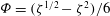
Figure 2. Shape function
 ${\it\Phi}({\it\zeta})$
versus reduced similarity variable for
${\it\Phi}({\it\zeta})$
versus reduced similarity variable for
 $n=0.2,0.4,0.6,0.8,1$
, and (a)
$n=0.2,0.4,0.6,0.8,1$
, and (a)
 ${\it\omega}={\it\gamma}=1$
; (b)
${\it\omega}={\it\gamma}=1$
; (b)
 ${\it\omega}=1.75,{\it\gamma}=1.25$
. The dots represent the analytical solution for a Newtonian fluid
${\it\omega}=1.75,{\it\gamma}=1.25$
. The dots represent the analytical solution for a Newtonian fluid
 $n=1$
(Barenblatt & Zel’dovich Reference Barenblatt and Zel’dovich1957).
$n=1$
(Barenblatt & Zel’dovich Reference Barenblatt and Zel’dovich1957).
Numerical results for the shape function
 ${\it\Phi}({\it\zeta})$
are shown as solid curves in figure 2 for different values of
${\it\Phi}({\it\zeta})$
are shown as solid curves in figure 2 for different values of
 $n$
representing shear-thinning fluids, and depicting cases with uniform permeability and porosity (figure 2
a) and with permeability and porosity increasing with
$n$
representing shear-thinning fluids, and depicting cases with uniform permeability and porosity (figure 2
a) and with permeability and porosity increasing with
 $z$
(figure 2
b). It is seen that the shape function tends to increase as
$z$
(figure 2
b). It is seen that the shape function tends to increase as
 $n$
decreases; this effect is compounded when the medium properties increase with elevation. For
$n$
decreases; this effect is compounded when the medium properties increase with elevation. For
 $n=1$
, the numerical solution is coincident with the analytical one, which exhibits a null height at the origin. For
$n=1$
, the numerical solution is coincident with the analytical one, which exhibits a null height at the origin. For
 $n<1$
, the shape function at
$n<1$
, the shape function at
 $x=0$
is non-zero and finite. This behaviour can be interpreted as the intermediate asymptotic of a process depending on
$x=0$
is non-zero and finite. This behaviour can be interpreted as the intermediate asymptotic of a process depending on
 $n,{\it\omega},{\it\gamma}$
and having a virtual origin at negative values of
$n,{\it\omega},{\it\gamma}$
and having a virtual origin at negative values of
 ${\it\zeta}$
; the solution evolves from a Dirac pulse at the initial stage with a left front end starting from zero and receding to meet the virtual origin. From that moment, the non-zero height condition at
${\it\zeta}$
; the solution evolves from a Dirac pulse at the initial stage with a left front end starting from zero and receding to meet the virtual origin. From that moment, the non-zero height condition at
 ${\it\zeta}=0$
applies (see Barenblatt & Vazquez Reference Barenblatt and Vazquez1998). The value of the shape function at the origin
${\it\zeta}=0$
applies (see Barenblatt & Vazquez Reference Barenblatt and Vazquez1998). The value of the shape function at the origin
 ${\it\Phi}(0)$
for shear-thinning fluids increases as
${\it\Phi}(0)$
for shear-thinning fluids increases as
 $n$
decreases, as illustrated in figure 3(a); the decrease is more evident for low values of
$n$
decreases, as illustrated in figure 3(a); the decrease is more evident for low values of
 $n$
, i.e. very strongly shear-thinning fluids. Figure 3(a) also plots the multiplicative constant
$n$
, i.e. very strongly shear-thinning fluids. Figure 3(a) also plots the multiplicative constant
 ${\it\eta}_{N}$
as a function of
${\it\eta}_{N}$
as a function of
 $n$
evaluated from the numerical solution using (3.4);
$n$
evaluated from the numerical solution using (3.4);
 ${\it\eta}_{N}$
tends to increase with increasing values of
${\it\eta}_{N}$
tends to increase with increasing values of
 $n$
. The actual behaviour of the current in terms of extension and height is best analysed in dimensional coordinates, as the scales adopted to obtain the dimensionless solution are themselves a function of model parameters.
$n$
. The actual behaviour of the current in terms of extension and height is best analysed in dimensional coordinates, as the scales adopted to obtain the dimensionless solution are themselves a function of model parameters.

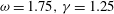
Figure 3. (a) Similarity variable at the current front
 ${\it\eta}_{N}$
and shape function in the origin
${\it\eta}_{N}$
and shape function in the origin
 ${\it\Phi}(0)$
versus
${\it\Phi}(0)$
versus
 $n$
for shear-thinning power-law fluids with different conditions for porosity and permeability vertical variations. (b) The flux draining from the current
$n$
for shear-thinning power-law fluids with different conditions for porosity and permeability vertical variations. (b) The flux draining from the current
 $R_{0}$
and the volume of the mound
$R_{0}$
and the volume of the mound
 $V$
as a function of time for
$V$
as a function of time for
 $n=0.2,0.4,0.6,0.8,1$
. The dots represent the analytical solution for a Newtonian fluid (Barenblatt & Zel’dovich Reference Barenblatt and Zel’dovich1957).
$n=0.2,0.4,0.6,0.8,1$
. The dots represent the analytical solution for a Newtonian fluid (Barenblatt & Zel’dovich Reference Barenblatt and Zel’dovich1957).
Figure 3(b) depicts the flux into the source
 $R_{0}$
, and the current volume
$R_{0}$
, and the current volume
 $V$
, as a function of time for different values of
$V$
, as a function of time for different values of
 $n$
. It is seen that both the flux at the origin and the mound volume decrease as the mound spreads. The flux from the current is smaller for low values of
$n$
. It is seen that both the flux at the origin and the mound volume decrease as the mound spreads. The flux from the current is smaller for low values of
 $n$
; as a consequence, the mound volume and its height at the origin are larger. In both cases, the available analytical solution for Newtonian fluid flow in a homogeneous medium (Barenblatt & Zel’dovich Reference Barenblatt and Zel’dovich1957) is perfectly reproduced by the numerical results.
$n$
; as a consequence, the mound volume and its height at the origin are larger. In both cases, the available analytical solution for Newtonian fluid flow in a homogeneous medium (Barenblatt & Zel’dovich Reference Barenblatt and Zel’dovich1957) is perfectly reproduced by the numerical results.
The solution for shear-thickening fluids (
 $n>1$
) indicates a detached origin on the left for positive values of
$n>1$
) indicates a detached origin on the left for positive values of
 ${\it\zeta}$
, a condition also encountered by Barenblatt & Vazquez (Reference Barenblatt and Vazquez1998) (namely in their Problem 2, Draining problem). The self-similar solution would exist for a infinite time and the left origin would move to the right proportionally to
${\it\zeta}$
, a condition also encountered by Barenblatt & Vazquez (Reference Barenblatt and Vazquez1998) (namely in their Problem 2, Draining problem). The self-similar solution would exist for a infinite time and the left origin would move to the right proportionally to
 $T^{-F_{2}}$
with a flux expressed by (3.8), which should be zero since no drain can be provided. A preliminary test conducted with a shear-thickening fluid (cornstarch suspension) showed that there is no detachment of the left origin, hence the self-similar solution (3.1) yields physically meaningless results for
$T^{-F_{2}}$
with a flux expressed by (3.8), which should be zero since no drain can be provided. A preliminary test conducted with a shear-thickening fluid (cornstarch suspension) showed that there is no detachment of the left origin, hence the self-similar solution (3.1) yields physically meaningless results for
 $n>1$
and will not be considered further.
$n>1$
and will not be considered further.
4. Analogue Hele-Shaw model
The Hele-Shaw approximation, a classical approach in the study of viscous flow problems, is valid for laminar flow between two plates separated by a small gap. Analogue Hele-Shaw models are traditionally used for the study of two-dimensional porous media given the identity of the governing equations. Newtonian flow in a uniform Hele-Shaw cell of thickness
 $b$
models Darcy flow in a homogeneous medium of permeability
$b$
models Darcy flow in a homogeneous medium of permeability
 $k(b)=b^{2}/12$
. Newtonian flow in a V-shaped Hele-Shaw cell reproduces Darcy flow in a heterogeneous medium with both permeability and porosity power-law variations along the vertical direction (Zheng et al.
Reference Zheng, Soh, Huppert and Stone2013); the ratio between the exponents of permeability and porosity is necessarily equal to 3, a value appropriate to represent a fissured medium. The approximation was extended to non-Newtonian power-law fluids (e.g. Aronsson & Janfalk Reference Aronsson and Janfalk1992; Kondic, Palffy-Muhoray & Shelley Reference Kondic, Palffy-Muhoray and Shelley1996; King Reference King2000). Based on the similarity between the modified Darcy’s law (2.2)–(2.3) and the laminar flow between two plates separated by a gap with half-width
$k(b)=b^{2}/12$
. Newtonian flow in a V-shaped Hele-Shaw cell reproduces Darcy flow in a heterogeneous medium with both permeability and porosity power-law variations along the vertical direction (Zheng et al.
Reference Zheng, Soh, Huppert and Stone2013); the ratio between the exponents of permeability and porosity is necessarily equal to 3, a value appropriate to represent a fissured medium. The approximation was extended to non-Newtonian power-law fluids (e.g. Aronsson & Janfalk Reference Aronsson and Janfalk1992; Kondic, Palffy-Muhoray & Shelley Reference Kondic, Palffy-Muhoray and Shelley1996; King Reference King2000). Based on the similarity between the modified Darcy’s law (2.2)–(2.3) and the laminar flow between two plates separated by a gap with half-width
 $W$
varying along the vertical as
$W$
varying along the vertical as
 $W(z)=b_{0}z^{r}$
, the analogy between flow of a power-law fluid in a Hele-Shaw cell of variable gap (the ‘model’) and a two-dimensional heterogeneous porous medium (the ‘prototype’) can be developed. Mapping
$W(z)=b_{0}z^{r}$
, the analogy between flow of a power-law fluid in a Hele-Shaw cell of variable gap (the ‘model’) and a two-dimensional heterogeneous porous medium (the ‘prototype’) can be developed. Mapping
 $H_{v}\rightarrow H^{p}$
, where
$H_{v}\rightarrow H^{p}$
, where
 $H_{v}$
is the non-dimensional thickness of the current in the Hele-Shaw cell and
$H_{v}$
is the non-dimensional thickness of the current in the Hele-Shaw cell and
 $p>1$
(see appendix B for the details), the analogy requires the following correspondence amongst the parameters:
$p>1$
(see appendix B for the details), the analogy requires the following correspondence amongst the parameters:
 $$\begin{eqnarray}\left\{\begin{array}{@{}l@{}}{\it\gamma}=p(r+1)\\ {\it\omega}={\displaystyle \frac{3pr(n+1)+p(n+3)-2}{n+1}}\\ n=n_{v},\end{array}\right.\end{eqnarray}$$
or, in terms of
 $p$
and
$p$
and
 $r$
:
$r$
:
 $$\begin{eqnarray}\left\{\begin{array}{@{}l@{}}p={\displaystyle \frac{(3{\it\gamma}-{\it\omega})(n+1)-2}{2n}}\\ r={\displaystyle \frac{{\it\omega}(n+1)-{\it\gamma}(n+3)+2}{(3{\it\gamma}-{\it\omega})(n+1)-2}}\\ n=n_{v},\end{array}\right.\end{eqnarray}$$
where
 $n_{v}$
is the behaviour index of the fluid used in the Hele-Shaw cell. It is seen that in all cases the analogy requires fluids with the same behaviour index in the prototype and in the model. For the other parameters, a parallel plate Hele-Shaw cell (
$n_{v}$
is the behaviour index of the fluid used in the Hele-Shaw cell. It is seen that in all cases the analogy requires fluids with the same behaviour index in the prototype and in the model. For the other parameters, a parallel plate Hele-Shaw cell (
 $r=0$
) represents flow in a porous medium with a variation of properties described by
$r=0$
) represents flow in a porous medium with a variation of properties described by
 $({\it\omega}-1)/({\it\gamma}-1)=(n+3)/(n+1)$
. This ratio: (i) tends to a value of
$({\it\omega}-1)/({\it\gamma}-1)=(n+3)/(n+1)$
. This ratio: (i) tends to a value of
 $3$
, typical of fissure networks, for very strongly shear-thinning fluids with
$3$
, typical of fissure networks, for very strongly shear-thinning fluids with
 $n\ll 1$
; (ii) is equal to
$n\ll 1$
; (ii) is equal to
 $2$
, typical of tubular flow paths, for
$2$
, typical of tubular flow paths, for
 $n=1$
; and (iii) is lower than
$n=1$
; and (iii) is lower than
 $2$
for shear-thickening fluids with
$2$
for shear-thickening fluids with
 $n>1$
. Mapping with
$n>1$
. Mapping with
 $p=1$
can only reproduce a fixed ratio
$p=1$
can only reproduce a fixed ratio
 $({\it\omega}-1)/({\it\gamma}-1)=3$
, corresponding to fissure networks and irrespective of the fluid behaviour index
$({\it\omega}-1)/({\it\gamma}-1)=3$
, corresponding to fissure networks and irrespective of the fluid behaviour index
 $n$
; for example, a cell with
$n$
; for example, a cell with
 $r=0.5$
reproduces the case
$r=0.5$
reproduces the case
 ${\it\omega}=2.5$
and
${\it\omega}=2.5$
and
 ${\it\gamma}=1.5$
. Figure 4 shows the possible combinations of parameters to ensure the analogy for fixed values of
${\it\gamma}=1.5$
. Figure 4 shows the possible combinations of parameters to ensure the analogy for fixed values of
 $n$
corresponding to Newtonian and shear-thinning fluids (
$n$
corresponding to Newtonian and shear-thinning fluids (
 $n=0.5$
), considering: (i) positive values of
$n=0.5$
), considering: (i) positive values of
 $({\it\omega}-1)$
and
$({\it\omega}-1)$
and
 $({\it\gamma}-1)$
, implying an increase of properties with elevation, the most plausible case in real porous media; (ii) a positive value of the mapping parameter
$({\it\gamma}-1)$
, implying an increase of properties with elevation, the most plausible case in real porous media; (ii) a positive value of the mapping parameter
 $p$
, to avoid singularities at the front end, where
$p$
, to avoid singularities at the front end, where
 $H=0$
; and (iii) a shape parameter of the cell
$H=0$
; and (iii) a shape parameter of the cell
 $0<r<1$
, equivalent to a moderate (less than linear) increase of the gap with elevation. Inspection of the figure 4 shows the combination of parameters satisfying the limitations
$0<r<1$
, equivalent to a moderate (less than linear) increase of the gap with elevation. Inspection of the figure 4 shows the combination of parameters satisfying the limitations
 $2\leqslant ({\it\omega}-1)/({\it\gamma}-1)\leqslant 3$
and
$2\leqslant ({\it\omega}-1)/({\it\gamma}-1)\leqslant 3$
and
 $p>0$
; the former constraint is more severe.
$p>0$
; the former constraint is more severe.

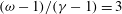
Figure 4. Interplay among parameters for Hele-Shaw analogue of flow in heterogeneous porous media with power-law permeability
 $k\propto z^{{\it\omega}-1}$
and porosity
$k\propto z^{{\it\omega}-1}$
and porosity
 ${\it\phi}\propto z^{{\it\gamma}-1}$
variations in the vertical direction (a) for Newtonian fluid (
${\it\phi}\propto z^{{\it\gamma}-1}$
variations in the vertical direction (a) for Newtonian fluid (
 $n=1$
); (b) for shear-thinning fluid (
$n=1$
); (b) for shear-thinning fluid (
 $n=0.5$
). Dashed lines represent isovalues of
$n=0.5$
). Dashed lines represent isovalues of
 $p$
, bold lines are isovalues of
$p$
, bold lines are isovalues of
 $r$
; the isovalue
$r$
; the isovalue
 $p=1$
is not affected by fluid behaviour index
$p=1$
is not affected by fluid behaviour index
 $n$
. The closed hatched area (yellow online) represents a positive ratio between permeability and porosity exponents in the range 2–3 with positive values of
$n$
. The closed hatched area (yellow online) represents a positive ratio between permeability and porosity exponents in the range 2–3 with positive values of
 $p$
; in the closed cross-hatched area (grey online)
$p$
; in the closed cross-hatched area (grey online)
 $p$
is also positive but
$p$
is also positive but
 $({\it\omega}-1)/({\it\gamma}-1)>3$
.
$({\it\omega}-1)/({\it\gamma}-1)>3$
.
5. Experiments
A series of experiments were conducted to compare with the theoretical work. The fluids were obtained by mixing glycerol, water and Xanthan gum in different ratios. In particular, 60 % (vol) glycerol, 40 % (vol) water and 0.1 % (weight) Xantham gum resulted in a fluid with
 $n=0.42$
; 70 % (vol) glycerol, 30 % (vol) water and 0.1 % (weight) Xantham gum resulted in a fluid with
$n=0.42$
; 70 % (vol) glycerol, 30 % (vol) water and 0.1 % (weight) Xantham gum resulted in a fluid with
 $n=0.47$
; 70 % (vol) glycerol, 30 % (vol) water and 0.06 % (weight) Xantham gum resulted in a fluid with
$n=0.47$
; 70 % (vol) glycerol, 30 % (vol) water and 0.06 % (weight) Xantham gum resulted in a fluid with
 $n=0.57$
. The Newtonian fluid was 95 % glycerol and 5 % water. The components were mixed and added with ink to enable an easy visualization of the current. The mixture was filtered in order to eliminate lumps and was stored in closed containers to avoid absorbing moisture. In general, the elimination of the lumps reduces the concentration of the Xantham gum with respect to the nominal mass fraction originally added. It is a source of variability in
$n=0.57$
. The Newtonian fluid was 95 % glycerol and 5 % water. The components were mixed and added with ink to enable an easy visualization of the current. The mixture was filtered in order to eliminate lumps and was stored in closed containers to avoid absorbing moisture. In general, the elimination of the lumps reduces the concentration of the Xantham gum with respect to the nominal mass fraction originally added. It is a source of variability in
 $n$
between different mixtures with the same nominal mass fraction of Xanthan gum.
$n$
between different mixtures with the same nominal mass fraction of Xanthan gum.
The rheological parameters were measured independently with a strain controlled parallel plate rheometer (Dynamic Shear Rheometer Anton Paar Physica MCR 101) in the low shear rate range (
 $\dot{{\it\gamma}}<5~\text{s}^{-1}$
), with associated uncertainty equal to 2.9 % and 3.1 % for the fluid behaviour and consistency indexes, respectively. The error bounds are the prediction intervals at 95 % confidence level.
$\dot{{\it\gamma}}<5~\text{s}^{-1}$
), with associated uncertainty equal to 2.9 % and 3.1 % for the fluid behaviour and consistency indexes, respectively. The error bounds are the prediction intervals at 95 % confidence level.

Figure 5. The apparent viscosity
 ${\it\mu}\equiv \widetilde{{\it\mu}}|\dot{{\it\gamma}}|^{n-1}$
as a function of shear rate; the rheometric test refers to the fluid used in Experiments 8–10. The bold line indicates the least squares regression for the low shear rate range, the dashed curves represent the prediction limit at 95 % of confidence level.
${\it\mu}\equiv \widetilde{{\it\mu}}|\dot{{\it\gamma}}|^{n-1}$
as a function of shear rate; the rheometric test refers to the fluid used in Experiments 8–10. The bold line indicates the least squares regression for the low shear rate range, the dashed curves represent the prediction limit at 95 % of confidence level.
Figure 5 shows the experimental data (apparent viscosity as a function of shear rate) and the fitting curve with the prediction interval for the fluid used in Experiments 8–10. A discussion on the methodology adopted for assessing the rheological parameters of the fluids is reported in Longo et al. (Reference Longo, Di Federico, Archetti, Chiapponi, Ciriello and Ungarish2013a ). The mass density was measured by a hydrometer (STV3500/23 Salmoiraghi) with an accuracy of 0.5 %.
Two different Hele-Shaw cells were used: the first had a constant gap of 3 mm or 3.2 mm; the second cell was V-shaped; the linearly varying gap reproduced a porous medium with a cubic variation of permeability and a linear variation of porosity along the vertical (
 ${\it\omega}=4,{\it\gamma}=2$
). Two vertical lock gates were used to confine the liquid. The lock gates were removed fast and the liquid spread along the cell and drained from the open end of the cell. The geometry of the current at different times was recorded by image analysis of frames recorded by a high-resolution video camera (1980
${\it\omega}=4,{\it\gamma}=2$
). Two vertical lock gates were used to confine the liquid. The lock gates were removed fast and the liquid spread along the cell and drained from the open end of the cell. The geometry of the current at different times was recorded by image analysis of frames recorded by a high-resolution video camera (1980
 $\times$
1080 pixels) recording at 25 frames
$\times$
1080 pixels) recording at 25 frames
 $\text{s}^{-1}$
and with a spatial resolution of 3 pixel
$\text{s}^{-1}$
and with a spatial resolution of 3 pixel
 $\text{mm}^{-1}$
. The images were processed with a proprietary software in order to obtain a planar restitution and to extract the coordinates of the boundary between the dark current and the white background. The overall uncertainty was of
$\text{mm}^{-1}$
. The images were processed with a proprietary software in order to obtain a planar restitution and to extract the coordinates of the boundary between the dark current and the white background. The overall uncertainty was of
 $\pm 1~\text{mm}$
.
$\pm 1~\text{mm}$
.
The parameters for all experiments are listed in table 1. Two experiments (no. 2 and no. 7) were carried out with a Newtonian fluid to calibrate the two cells. The front position as function of the time for all experiments is shown in figure 6(a). The relevant differences between theory and experiment during the initial stage of propagation were mainly due to the finite size of the mound at
 $t=0$
; the slumping phase is relatively short due to the rapid dominance of viscous effects over inertial ones. At intermediate times, experimental data collapse onto the theoretical line. At long times, the current becomes thinner and the effect of the friction at the bottom of the cell becomes non-negligible; this is reflected in a reduction of the speed of the current, with a consequent overestimation of the theoretical speed. For most tests, the intermediate times are a multiple of the time scale (the time scale is generally less than 0.5 second), hence self-similarity develops after a few seconds from the opening of the locks. The long times depend on the factors determining the discrepancies between the model and the experiment. For the present tests, long times mean several tens of seconds.
$t=0$
; the slumping phase is relatively short due to the rapid dominance of viscous effects over inertial ones. At intermediate times, experimental data collapse onto the theoretical line. At long times, the current becomes thinner and the effect of the friction at the bottom of the cell becomes non-negligible; this is reflected in a reduction of the speed of the current, with a consequent overestimation of the theoretical speed. For most tests, the intermediate times are a multiple of the time scale (the time scale is generally less than 0.5 second), hence self-similarity develops after a few seconds from the opening of the locks. The long times depend on the factors determining the discrepancies between the model and the experiment. For the present tests, long times mean several tens of seconds.
For a more detailed analysis of the uncertainties in the results of the model as a function of the uncertainties in the parameters, the methodology described in Di Federico et al. (Reference Di Federico, Longo, Chiapponi, Archetti and Ciriello2014) can be applied. Figure 6(b) shows the dipole moment as function of time for three selected experiments (numbers 8, 9, and 10), characterised by initial aspect ratios (ratio of the initial height to initial length of the fluid behind the lock gates) equal to
 $0.8,1.5$
and
$0.8,1.5$
and
 $0.72$
, respectively. After an initial slumping phase, the moment tends to a constant, as predicted by the theory. The moment was estimated by fitting the experimental points representing the boundary of the current (detected with the video image analysis) and then integrating the fitting function. The uncertainty in the dipole moment has been evaluated with a Monte Carlo simulation, by (i) generating several samples of points (
$0.72$
, respectively. After an initial slumping phase, the moment tends to a constant, as predicted by the theory. The moment was estimated by fitting the experimental points representing the boundary of the current (detected with the video image analysis) and then integrating the fitting function. The uncertainty in the dipole moment has been evaluated with a Monte Carlo simulation, by (i) generating several samples of points (
 $10\,000$
samples) representing the boundary, by assuming a Gaussian distribution with variance equal to 1 mm around the experimental value; (ii) fitting the synthetic samples and integrating the fitting curves; and (iii) computing the variance of the samples of the results of the integration. A comparison of the experimental profile with theory is shown in figure 7(a). Near the origin, the height of the current is non-zero, as predicted by the theory. Near the front, capillarity effects not included in the theory produce an underestimation of the height and of the front position. Elsewhere, the agreement between theory and experiments is remarkably good at intermediate and late times, indicating that the current converges to the self-similar regime. A balance between two counteracting effects not included in the model, i.e. the depression of the current associated with the vertical velocity and capillarity, probably contributes to the excellent fit.
$10\,000$
samples) representing the boundary, by assuming a Gaussian distribution with variance equal to 1 mm around the experimental value; (ii) fitting the synthetic samples and integrating the fitting curves; and (iii) computing the variance of the samples of the results of the integration. A comparison of the experimental profile with theory is shown in figure 7(a). Near the origin, the height of the current is non-zero, as predicted by the theory. Near the front, capillarity effects not included in the theory produce an underestimation of the height and of the front position. Elsewhere, the agreement between theory and experiments is remarkably good at intermediate and late times, indicating that the current converges to the self-similar regime. A balance between two counteracting effects not included in the model, i.e. the depression of the current associated with the vertical velocity and capillarity, probably contributes to the excellent fit.
Table 1. Experimental parameters for all Experiments in Hele-Shaw cells. The last three Experiments are in a V shaped Hele-Shaw cell, reproducing flow in a porous medium with a cubic variation of permeability and a linear variation of porosity along the vertical. A power of the dipole moment (dimensions [
 $L^{{\it\gamma}+2}$
]) is listed. The nominal value of the dipole moment
$L^{{\it\gamma}+2}$
]) is listed. The nominal value of the dipole moment
 $Q_{0}$
was computed from the initial state at rest, by digitizing the images before opening the locks.
$Q_{0}$
was computed from the initial state at rest, by digitizing the images before opening the locks.


Figure 6. (a) Experimental front positions (symbols) and theoretical predictions (solid lines)
 $X_{N}$
against time
$X_{N}$
against time
 $T$
. The variables
$T$
. The variables
 $X_{N}$
and
$X_{N}$
and
 $T$
are non-dimensional and
$T$
are non-dimensional and
 $X_{N}$
is scaled according to
$X_{N}$
is scaled according to
 $f(X_{N})=(X_{N}/{\it\eta}_{N})^{1/[{\it\gamma}n/({\it\omega}(n+1)+2)]}$
. The data for experiments in the V-shaped cell are multiplied by a factor 2 in order to be separated from the data for the constant gap cell. For clarity, one point out of three is plotted. (b) Experimental dipole moment for three experiments with aspect ratio
$f(X_{N})=(X_{N}/{\it\eta}_{N})^{1/[{\it\gamma}n/({\it\omega}(n+1)+2)]}$
. The data for experiments in the V-shaped cell are multiplied by a factor 2 in order to be separated from the data for the constant gap cell. For clarity, one point out of three is plotted. (b) Experimental dipole moment for three experiments with aspect ratio
 $0.8,1.5$
, and
$0.8,1.5$
, and
 $0.72$
, respectively.
$0.72$
, respectively.
 $Q_{0}$
is the nominal dipole moment at time
$Q_{0}$
is the nominal dipole moment at time
 $t=0$
. The error bar shown indicates a single standard deviation.
$t=0$
. The error bar shown indicates a single standard deviation.

Figure 7. Experiment no. 16 (a) Photographs showing the current profiles at various times since release (10, 30, 50, 70 and 90 s) in a V-shaped Hele-Shaw cell. The curves with symbols represent the theoretical profile. The vertical dashed lines are 10 cm apart. (b) The dimensionless volume of fluid drained at the origin
 $V_{out}$
(defined by (3.10)) plotted against
$V_{out}$
(defined by (3.10)) plotted against
 $T^{-F_{2}}\equiv T^{-0.119}$
(filled symbols) and the dimensionless (scaled with
$T^{-F_{2}}\equiv T^{-0.119}$
(filled symbols) and the dimensionless (scaled with
 $x_{\ast }$
) height of the current in the origin plotted against
$x_{\ast }$
) height of the current in the origin plotted against
 $T^{F_{3}}\equiv T^{-F_{2}}$
(empty symbols). The time increases toward the origin. The error bars indicate a single standard deviation.
$T^{F_{3}}\equiv T^{-F_{2}}$
(empty symbols). The time increases toward the origin. The error bars indicate a single standard deviation.
Finally, we investigate the current behaviour at the origin by plotting the volume of fluid drained
 $V_{out}$
, and the height
$V_{out}$
, and the height
 $H_{0}$
against time for Experiment no. 16 (figure 7
b). Theoretically,
$H_{0}$
against time for Experiment no. 16 (figure 7
b). Theoretically,
 $V_{out}$
and
$V_{out}$
and
 $H_{0}$
are proportional to
$H_{0}$
are proportional to
 $T^{F_{2}}$
and
$T^{F_{2}}$
and
 $T^{-F_{3}}$
respectively. In the selected case,
$T^{-F_{3}}$
respectively. In the selected case,
 $F_{3}=-F_{2}$
as
$F_{3}=-F_{2}$
as
 ${\it\gamma}=2$
, hence the same exponent is expected experimentally for the two plots except for the sign. Inspection of figure 7(b) confirms the theory for intermediate and late times. Similar plots are obtained for the other experiments.
${\it\gamma}=2$
, hence the same exponent is expected experimentally for the two plots except for the sign. Inspection of figure 7(b) confirms the theory for intermediate and late times. Similar plots are obtained for the other experiments.
6. Conclusions
We have analysed the intermediate asymptotic behaviour of a mound of power-law shear-thinning fluid propagating in a two-dimensional porous medium freely draining at one end, considering constant or vertically varying porosity and permeability according to a power-law relationship. This type of variation mimics the sub-horizontal stratifications of porous media, or the change in fracture density with depth of densely fractured media. A similarity solution has been derived in closed form, extending in two respects the work of King & Woods (Reference King and Woods2003), who treated the dipole flow for a Newtonian fluid and vertically variable permeability. The dipole moment of the flow is conserved with a non-zero height of the current at the origin. We have established an analogy with the flow of a fluid with the same behaviour index in a Hele-Shaw cell with half-gap varying in the vertical as
 $W(z)=b_{0}z^{r}$
, representing a variety of combinations of porosity and permeability. The general Hele-Shaw analogue provides a useful tool for the experimental simulation of power-law free-surface flows in porous media. A set of experiments based on this analogy were conducted in a constant gap (
$W(z)=b_{0}z^{r}$
, representing a variety of combinations of porosity and permeability. The general Hele-Shaw analogue provides a useful tool for the experimental simulation of power-law free-surface flows in porous media. A set of experiments based on this analogy were conducted in a constant gap (
 $r=0$
) and V-shaped cell (
$r=0$
) and V-shaped cell (
 $r=1$
). The time series of the front-end position, dipole moment, drained volume and height at the origin, as well as the current profiles, agreed well with the theoretical predictions at intermediate and late times. Our results demonstrate that the combined effect of fluid rheology and spatial variations of medium properties significantly affect the current extension and profile, and extend the available body of knowledge on non-Newtonian flow in porous media, a topic of interest for its environmental and industrial implications.
$r=1$
). The time series of the front-end position, dipole moment, drained volume and height at the origin, as well as the current profiles, agreed well with the theoretical predictions at intermediate and late times. Our results demonstrate that the combined effect of fluid rheology and spatial variations of medium properties significantly affect the current extension and profile, and extend the available body of knowledge on non-Newtonian flow in porous media, a topic of interest for its environmental and industrial implications.
Acknowledgements
We thank the anonymous reviewers for their useful comments and suggestions that helped in improving the quality and the readability of the manuscript.
Appendix A. The integration of the differential problem
The integration of the differential problem in (3.3)–(3.5) can be obtained with standard numerical algorithms (we used those implemented in Wolfram Mathematica® 10) and requires an extra condition near the front end. Here, for
 ${\it\zeta}\rightarrow 1-{\it\epsilon}$
the power series expansion of the shape function yields
${\it\zeta}\rightarrow 1-{\it\epsilon}$
the power series expansion of the shape function yields
 $$\begin{eqnarray}\displaystyle & \displaystyle {\it\Phi}({\it\epsilon})=\left({\displaystyle \frac{F_{2}}{{\it\gamma}F_{5}^{1/n}}}\right)^{nF_{5}}{\it\epsilon}^{F_{5}}, & \displaystyle\end{eqnarray}$$
 $$\begin{eqnarray}\displaystyle & \displaystyle {\it\Phi}^{\prime }({\it\epsilon})=-F_{5}\left({\displaystyle \frac{F_{2}}{{\it\gamma}F_{5}^{1/n}}}\right)^{nF_{5}}{\it\epsilon}^{F_{5}-1}, & \displaystyle\end{eqnarray}$$
 $$\begin{eqnarray}F_{5}={\displaystyle \frac{2}{({\it\omega}-{\it\gamma})(n+1)+2}},\end{eqnarray}$$
and
 ${\it\epsilon}$
is a small positive quantity (
${\it\epsilon}$
is a small positive quantity (
 ${\it\epsilon}=10^{-6}$
–
${\it\epsilon}=10^{-6}$
–
 $10^{-8}$
in most computations). However, numerical instabilities develop near the maximum for
$10^{-8}$
in most computations). However, numerical instabilities develop near the maximum for
 $n\neq 1$
due to the absolute value operator in (3.3). These instabilities can be overcome by increasing the accuracy and the precision in the algorithm application. For small
$n\neq 1$
due to the absolute value operator in (3.3). These instabilities can be overcome by increasing the accuracy and the precision in the algorithm application. For small
 $n$
, we found it more efficient to split the integration into a right branch from
$n$
, we found it more efficient to split the integration into a right branch from
 ${\it\zeta}=1$
to
${\it\zeta}=1$
to
 ${\it\zeta}={\it\zeta}_{M}$
(
${\it\zeta}={\it\zeta}_{M}$
(
 ${\it\zeta}_{M}$
is the abscissa where the maximum value
${\it\zeta}_{M}$
is the abscissa where the maximum value
 ${\it\Phi}_{M}$
occurs), and a left branch from
${\it\Phi}_{M}$
occurs), and a left branch from
 ${\it\zeta}={\it\zeta}_{M}$
to
${\it\zeta}={\it\zeta}_{M}$
to
 ${\it\zeta}=0$
. A series expansion of the shape function near
${\it\zeta}=0$
. A series expansion of the shape function near
 ${\it\zeta}_{M}$
, valid for
${\it\zeta}_{M}$
, valid for
 $n<1$
gives
$n<1$
gives
 $$\begin{eqnarray}\displaystyle & \displaystyle {\it\Phi}({\it\zeta}_{M}-{\it\epsilon})={\it\Phi}_{M}-\left({\displaystyle \frac{(1-n)^{1/n}F_{2}{\it\zeta}_{M}}{{\it\Phi}_{M}^{1+F_{1}-{\it\gamma}}}}\right)^{n/(1-n)}{\it\zeta}_{M}^{1/(1-n)}{\it\epsilon}^{1/(1-n)}, & \displaystyle\end{eqnarray}$$
 $$\begin{eqnarray}\displaystyle & \displaystyle {\it\Phi}^{\prime }({\it\zeta}_{M}-{\it\epsilon})={\displaystyle \frac{1}{1-n}}\left({\displaystyle \frac{(1-n)^{1/n}F_{2}{\it\zeta}_{M}}{{\it\Phi}_{M}^{1+F_{1}-{\it\gamma}}}}\right)^{n/(1-n)}{\it\zeta}_{M}^{n/(1-n)}{\it\epsilon}^{n/(1-n)}. & \displaystyle\end{eqnarray}$$
Appendix B. Analogue Hele-Shaw model of power-law fluid in a porous medium
In developing the present analogy, we assume that the cell gap and the porous medium properties (permeability and porosity) are constant in the horizontal direction (parallel to the flow), and vary in the vertical direction (transverse to the flow). We consider the momentum and local mass balance equations for a gravity current of a power-law fluid between two surfaces with varying half-width along the vertical, given by the monomial expression
 $W(x)=b_{0}z^{r}$
. The hypothesis of no slip conditions at the rigid walls leads to the following partial differential equation for the height of the current
$W(x)=b_{0}z^{r}$
. The hypothesis of no slip conditions at the rigid walls leads to the following partial differential equation for the height of the current
 $$\begin{eqnarray}\displaystyle \frac{\partial h_{v}^{r+1}}{\partial t} & = & \displaystyle \left[\left(\frac{{\rm\Delta}{\it\rho}_{v}g}{\widetilde{{\it\mu}}_{v}}\right)^{1/n_{v}}\frac{n_{v}^{2}(r+1)}{[r(2n_{v}+1)+n_{v}](2n_{v}+1)}b_{0}^{(n_{v}+1)/n_{v}}\right]\nonumber\\ \displaystyle & & \displaystyle \times \,\frac{\partial }{\partial x}\left[h_{v}^{1+r(2n_{v}+1)/n_{v}}\frac{\partial h_{v}}{\partial x}\left|\frac{\partial h_{v}}{\partial x}\right|^{1/n_{v}-1}\right],\end{eqnarray}$$
where the subscript
 $v$
refers to the Hele-Shaw cell, which is to be solved with the boundary condition at the front end
$v$
refers to the Hele-Shaw cell, which is to be solved with the boundary condition at the front end
 $h_{v}(x_{N}(t),t)=0$
and respecting the integral constraint
$h_{v}(x_{N}(t),t)=0$
and respecting the integral constraint
 $$\begin{eqnarray}\frac{2b_{0}}{r+1}\int _{0}^{x_{N}(t)}xh_{v}^{r+1}\,\text{d}x=Q_{v},\end{eqnarray}$$
where
 $Q_{v}$
, having dimensions
$Q_{v}$
, having dimensions
 $[L^{3+r}]$
, is the constant dipole moment. By introducing the following length and velocity scales
$[L^{3+r}]$
, is the constant dipole moment. By introducing the following length and velocity scales
 $$\begin{eqnarray}\displaystyle & \displaystyle x_{v}^{\ast }=\left(\frac{r+1}{2b_{0}}Q_{v}\right)^{1/(r+3)} & \displaystyle\end{eqnarray}$$
 $$\begin{eqnarray}\displaystyle & \displaystyle u_{v}^{\ast }=\left(\frac{{\rm\Delta}{\it\rho}_{v}g}{\widetilde{{\it\mu}}_{v}}\right)^{1/n_{v}}\frac{n_{v}^{2}(r+1)p^{1/n_{v}}}{[r(2n_{v}+1)+n_{v}](2n_{v}+1)}\left(\frac{r+1}{2}b_{0}^{3/r}Q_{v}\right)^{r(n_{v}+1)/[n_{v}(r+3)]}, & \displaystyle\end{eqnarray}$$
 $p^{1/n_{v}}(p>0)$
is introduced for convenience, (B 1)–(B 2) become
$p^{1/n_{v}}(p>0)$
is introduced for convenience, (B 1)–(B 2) become  $$\begin{eqnarray}\displaystyle & \displaystyle \frac{\partial h_{v}^{r+1}}{\partial t}=\frac{u_{v}^{\ast }}{x_{v}^{\ast r(n_{v}+1)/n_{v}}p^{1/n_{v}}}\frac{\partial }{\partial x}\left[h_{v}^{1+r(2n_{v}+1)/n_{v}}\frac{\partial h_{v}}{\partial x}\left|\frac{\partial h_{v}}{\partial x}\right|^{1/n_{v}-1}\right], & \displaystyle\end{eqnarray}$$
 $$\begin{eqnarray}\displaystyle & \displaystyle \frac{1}{x_{v}^{\ast r+3}}\int _{0}^{x_{N}(t)}xh_{v}^{r+1}\,\text{d}x=1. & \displaystyle\end{eqnarray}$$
 $$\begin{eqnarray}\displaystyle & \displaystyle \frac{\partial H_{v}^{r+1}}{\partial T}=\frac{1}{p^{1/n_{v}}}\frac{}{}\frac{\partial }{\partial X}\left[H_{v}^{1+r(2n_{v}+1)/n_{v}}\frac{\partial H_{v}}{\partial X}\left|\frac{\partial H_{v}}{\partial X}\right|^{1/n_{v}-1}\right], & \displaystyle\end{eqnarray}$$
 $$\begin{eqnarray}\displaystyle & \displaystyle \int _{0}^{X_{N}(T)}XH_{v}^{r+1}\,\text{d}X=1. & \displaystyle\end{eqnarray}$$
Mapping
 $H_{v}\rightarrow H^{p}$
transforms (B 7)–(B 8) into
$H_{v}\rightarrow H^{p}$
transforms (B 7)–(B 8) into
 $$\begin{eqnarray}\displaystyle & \displaystyle \frac{\partial H^{p(r+1)}}{\partial T}=\frac{\partial }{\partial X}\left[H^{p[1+r(2n_{v}+1)/n_{v}]+(p-1)/n_{v}}\frac{\partial H}{\partial X}\left|\frac{\partial H}{\partial X}\right|^{1/n_{v}-1}\right], & \displaystyle\end{eqnarray}$$
 $$\begin{eqnarray}\displaystyle & \displaystyle \int _{0}^{X_{N}(T)}XH^{p(r+1)}\,\text{d}X=1. & \displaystyle\end{eqnarray}$$
The analogy between the model Hele-Shaw flow described by (B 9)–(B 10) and the prototype porous flow described by (2.13)–(2.14), requires the corresponding terms in the differential and integral expressions to be identical. Equating the exponents yields the solutions shown in (4.1) and (4.2). The established analogy allows for the performance of experiments in a Hele-Shaw cell and the transformation of the experimental results obtained (the measured height of the current and the time series of the front end position) into equivalent results for the mound spreading in a porous medium.


