2. Problem set-up

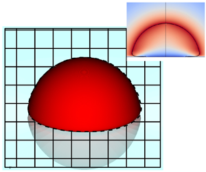
We numerically study the response of a spherical cap nucleus to a sudden drop in system pressure using the set-up shown in figure 1. We restrict ourselves to an axisymmetric configuration where the initial bubble pressure $p_{g,0}$ is uniform inside the bubble and the liquid, initially at rest, is suddenly exposed to a lower pressure far from the bubble $p_\infty < p_{g,0}$. This problem corresponds to a regime where the bubble growth is predominantly controlled by the inertial effects as the heat and the mass diffusion effects are neglected. Consequently, our study is valid at short times after the bubble nucleation, particularly $t < L_{\mathcal {D}}^2/\mathcal {D}$, where $L_{\mathcal {D}}$ is a characteristic length for diffusion and $\mathcal {D}$ is the Fickian constant for the diffusion law of heat/mass transfer process (Bergamasco & Fuster Reference Bergamasco and Fuster2017; Sullivan et al. Reference Sullivan, Dockar, Borg, Enright and Pillai2022). To render the problem dimensionless, we define the initial bubble radius of curvature as a characteristic length $L_c = R_{c,0}$, the liquid density as a characteristic density $\rho _c = \rho _l$ and the asymptotic Rayleigh–Plesset velocity as a characteristic velocity of the problem $U_c = \sqrt {\frac {2}{3}({\Delta p}/{\rho })}$. The dynamics of these bubbles is governed by compressible Navier–Stokes equations which, for a two-phase ($i \in \{l,g\}$) system in a dimensionless form, reads

(2.1)$$\begin{gather} \frac{\partial \tilde{\rho}_i}{\partial \tilde{t}} + \boldsymbol{\nabla} \boldsymbol{\cdot} (\tilde{\rho}_i \tilde{{\boldsymbol u}}_i) = 0, \end{gather}$$

(2.2)$$\begin{gather}\frac{\partial \tilde{\rho}_i \tilde{{\boldsymbol u}}_i}{\partial \tilde{t}} + \boldsymbol{\nabla} \boldsymbol{\cdot} (\tilde{\rho}_i \tilde{{\boldsymbol u}}_i \tilde{{\boldsymbol u}}_i) + \boldsymbol{\nabla} \tilde{p}_i = \frac{{Oh}^2}{{Ca}} \boldsymbol{\nabla} \boldsymbol{\cdot} (2 \tilde{\mu}_i \tilde{\boldsymbol{D}}_i), \end{gather}$$

(2.3)$$\begin{gather}\frac{\partial (\tilde{\rho}_i \tilde{E}_i)}{\partial \tilde{t}} + \boldsymbol{\nabla} \boldsymbol{\cdot} (\tilde{\rho}_i \tilde{E}_i \tilde{\boldsymbol{u}}_i) + \boldsymbol{\nabla} \boldsymbol{\cdot} (\tilde{{\boldsymbol u}}_i \tilde{p}_i) = \frac{{Oh}^2}{{Ca}} \boldsymbol{\nabla} \boldsymbol{\cdot} (2 \tilde{\mu}_i \tilde{\boldsymbol{D}}_i) \tilde{{\boldsymbol u}}_i, \end{gather}$$

where the subscript ‘$i$’ represents the value of a particular variable for the $i$th component, ${Ca} = \mu _l U_c/\sigma$ is the capillary number, $\sigma$ is the surface-tension between the liquid and gas phase, $\mu _l$ is the liquid viscosity, ${Oh} = \mu _l/\sqrt {\rho _l \sigma R_{c,0}}$ is the Ohnesorge number, $\tilde {\boldsymbol {u}}$ is the dimensionless velocity vector field, $\tilde {\rho }$ is the dimensionless density, $\tilde {p}$ is the dimensionless pressure field, $\tilde {E}$ is the dimensionless total energy per unit volume which is defined as the sum of the internal energy and the kinetic energy $(\tilde {\rho }_i \tilde {e}_i + \frac {1}{2} \tilde {\rho }_i \tilde {\boldsymbol {u}}_i \boldsymbol {\cdot } \tilde {\boldsymbol {u}}_i)$, and $\tilde {\boldsymbol {D}}_i$ is the strain rate tensor.

Figure 1. A simplified schematic of the problem.

The system of equations is closed by an equation of state for each component. We use a stiffened gas equation of state (EOS) similar to that of Cocchi, Saurel & Loraud (Reference Cocchi, Saurel and Loraud1996), given as

(2.4)\begin{equation} \tilde{\rho}_i \tilde{e}_i = \frac{\tilde{p}_i + \tilde{\varGamma}_i \tilde{\varPi}_i}{\tilde{\varGamma}_i - 1},\end{equation}

where $\tilde {\varGamma }_i$ and $\tilde {\varPi }_i$ are empirical constants taken from Johnsen & Colonius (Reference Johnsen and Colonius2006) to replicate the speeds of sound in water and ideal gas. The interface between the two immiscible fluids is mathematically represented with the Heaviside function $(\mathcal {H})$ which takes the value 1 in the reference component and 0 in the non-reference component (Tryggvason, Scardovelli & Zaleski Reference Tryggvason, Scardovelli and Zaleski2011). The evolution of the interface is described by an advection equation

(2.5)\begin{equation} \frac{\partial \mathcal{H}}{\partial \tilde{t}} + \tilde{\boldsymbol{u}} \boldsymbol{\cdot} \boldsymbol{\nabla} \mathcal{H} = 0,\end{equation}

where $\tilde {\boldsymbol {u}}$ is the average local velocity of the interface which is imposed to be equal to local fluid velocity. The interface conditions are required to couple the motion of fluids in each component. In the absence of mass transfer effects, these conditions are as follows: the velocity is continuous across the interface such that $[\![\tilde {\boldsymbol {u}}]\!] = 0$, where $[\![{\cdot }]\!]$ represents the jump in the particular quantity across the interface. The pressure in both the components is related by the Laplace equation

(2.6)\begin{equation} \frac{1}{{Oh}^2}[\![\tilde{p}]\!] ={-} \frac{1}{{Ca}^2} \tilde{\kappa} + \frac{1}{{Ca}}[\![ \boldsymbol{n}_I \boldsymbol{\cdot} 2 \tilde{\mu} \tilde{\boldsymbol{D}} \boldsymbol{\cdot} \boldsymbol{n}_I ]\!],\end{equation}

where $\tilde {\kappa }$ is the dimensionless curvature of the interface and $\boldsymbol {n}_I$ is the unit vector normal to the interface. We also assume that there is no heat transfer across the interface, so the normal derivative of internal energy remains continuous across the interface i.e. $[\![\partial \tilde {e}/\partial n]\!] = 0.$

We integrate (2.1)–(2.3) and (2.5) (satisfying (2.4) and (2.6)) on the finite volume grids using the numerical method discussed by Fuster & Popinet (Reference Fuster and Popinet2018) also used by Fan, Li & Fuster (Reference Fan, Li and Fuster2020), Saini (Reference Saini2022), Saini et al. (Reference Saini, Tanne, Arrigoni, Zaleski and Fuster2022, Reference Saini, Saade, Fuster and Lohse2024) and extended to include thermal effects by Saade, Lohse & Fuster (Reference Saade, Lohse and Fuster2023). This method is implemented in the free software program called Basilisk (Popinet Reference Popinet2015). In this implementation, a geometric volume of fluid (VoF) method with piece-wise linear constructions in the discrete cells is used for the interface representation (Tryggvason et al. Reference Tryggvason, Scardovelli and Zaleski2011). In the VoF method, the phase characteristic function is represented with the colour function $C_i$ which is $1$ in the reference phase, $0$ in non-reference phase and in the cells containing both phases, $C_i$ takes fractional value between 0 and 1. The conserved quantities (density $C_i \tilde {\rho }_i$, momentum $C_i \tilde {\rho }_i \tilde {\boldsymbol {u}}_i$, total energy $C_i \tilde {\rho }_i \tilde {E}_i$) are advected consistently with the colour function (see Arrufat et al. Reference Arrufat, Crialesi, Fuster, Ling, Malan, Pal, Scardovelli, Tryggvason and Zaleski2021).

The capillary forces are added as continuum surface forces (CSFs) where the delta function is approximated as the gradient of colour function $\vert \boldsymbol {\nabla } C \vert$ (Brackbill, Kothe & Zemach Reference Brackbill, Kothe and Zemach1992; Popinet Reference Popinet2009, Reference Popinet2018). The primitive variables are density, momentum, total energy and the colour function leading to a density-based formulation where an auxiliary equation is solved to obtain a provisional value of the volume-averaged pressure $\tilde {p}_{{avg}}$ required to reconstruct the pressure of the individual phases required to compute the fluxes of the primitive quantities (Kwatra et al. Reference Kwatra, Su, Grétarsson and Fedkiw2009)

(2.7)\begin{equation} {\frac{1}{ \tilde{\rho}_{{avg}} \widetilde{c_e}^{2}}} \left( \frac{\partial \tilde{p}_{{avg}}}{\partial \tilde{t}} + \tilde{\boldsymbol{u}} \boldsymbol{\cdot} \boldsymbol{\nabla} \tilde{p}_{{avg}} \right) = \boldsymbol{\nabla \cdot} \tilde{\boldsymbol{u}},\end{equation}

where the subindex ‘avg’ stands for a volume-averaged quantity and $\tilde {c}_e$ is the effective speed of sound of the mixture. Note that generalized expressions of the equation above accounting for full viscous and thermal effects can be found from Saade et al. (Reference Saade, Lohse and Fuster2023) and Urbano, Bibal & Tanguy (Reference Urbano, Bibal and Tanguy2022). For more details about the details of the specific numerical method used here, the reader is referred to the work of Fuster & Popinet (Reference Fuster and Popinet2018).

Similar to the works of Afkhami et al. (Reference Afkhami, Buongiorno, Guion, Popinet, Saade, Scardovelli and Zaleski2018), Guion et al. (Reference Guion, Afkhami, Zaleski and Buongiorno2018), Kamal et al. (Reference Kamal, Sprittles, Snoeijer and Eggers2019) and Ming et al. (Reference Ming, Qin and Gao2023), the motion of the contact line is regularized by the Navier-slip model

(2.8)\begin{equation} \tilde{\boldsymbol{u}}^{\boldsymbol{T}} = \frac{\lambda_{num}}{R_{c,0}} \frac{\partial \tilde{\boldsymbol{u}}^{\boldsymbol{T}}}{\partial \boldsymbol{T}}, \end{equation}

where $\tilde {\boldsymbol {u}}^{\boldsymbol {T}}$ is the tangential velocity vector at the wall, $\boldsymbol {T}$ is unit vector tangent to the wall and $\lambda _{num}$ is the slip length. In this article, the slip length is fixed to $\lambda _{num} = 0.01 R_{c,0}$ unless mentioned otherwise. This choice is limited by the minimum grid size which is $\varDelta _{min} = 0.003 R_{c,0}$ in our case. Some results especially in the region very close to contact line can depend on this choice, however, the results in the microlayer region are independent (see the supplementary material available at https://doi.org/10.1017/jfm.2024.236). We also use a static contact angle model implemented using the approach of Afkhami & Bussmann (Reference Afkhami and Bussmann2008). For other boundaries, we have used reflective boundary conditions: $\tilde {\boldsymbol {u}}^{\boldsymbol {n}} = 0$, ${\partial \tilde {\boldsymbol {u}}^{\boldsymbol {T}}}/{\partial \boldsymbol {n}} = 0$, $\boldsymbol {n} \boldsymbol {\cdot } \boldsymbol {\nabla } \tilde {p} = 0$, where $\tilde {\boldsymbol {u}}^{\boldsymbol {n}}$ is the velocity vector normal to the wall and $\boldsymbol {n}$ is the unit vector normal to the wall. The numerical domain is made large enough ($100 R_{c,0} \times 100 R_{c,0}$) and the numerical grid is coarsened near the boundary to prevent any reflected waves from influencing the bubble dynamics.

3. Nucleation threshold

The nucleation threshold for the growth of a cavitation bubble from a small nuclei (air pocket) is the critical pressure beyond which this nuclei becomes unstable and grows explosively. This critical pressure can be predicted by quasi-static theory for bubble expansion, as shown by Atchley & Prosperetti (Reference Atchley and Prosperetti1989), Crum (Reference Crum1979), Fuster et al. (Reference Fuster, Pham and Zaleski2014) and many others. In the case of a hemispherical cap bubble attached to a flat wall, the critical pressure ($\kern 1.5pt p_{cr}$) is

(3.1)\begin{equation} \frac{p_{cr}}{p_{L,0}} ={-} \left(\frac{3}{2} \frac{p_{L,0}R_{c,0}}{\sigma} \gamma \left(1 + 2 \frac{\sigma}{p_{L,0}R_{c,0}} \right) \right)^{{1}/({1 - 3\gamma})} 2 \frac{\sigma}{p_{L,0}R_{c,0}} \left(1 - \frac{1}{3 \gamma}\right), \end{equation}

where $p_{L,0}$ is the initial liquid pressure just outside the interface and $\gamma = 1.4$ is the ratio of specific heats for air. For deriving this relation, we have assumed that the bubble contact angle remains 90$^\circ$ and that the contact line can freely move on the solid boundary. In a previous study (see Saini et al. Reference Saini, Zaleski and Fuster2021; Saini Reference Saini2022), we have shown that the change in contact angle and contact line motion imposes secondary effects on the nucleation threshold. Equation (3.1) can be converted to the $Ca$–$Oh$ plane where it imposes a region of stability such that for given ${Oh}$ (function of bubble size), there is a critical capillary number (function of critical pressure) beyond which a nuclei will become unstable. This critical capillary number is

(3.2)\begin{equation} {Ca}_c = {Oh} \sqrt{2 \left(1 - \frac{1}{3\gamma}\right) \left[\frac{3}{2} \left(\frac{{Ca}_0}{{Oh}}\right)^2 \gamma \left(1 + 2 \left(\frac{{Oh}}{{Ca}_0}\right)^2\right)\right]^{1/(1 - 3 \gamma)}}, \end{equation}

where ${Ca}_0$ is defined as ${Ca}_0 = ({\mu _l}/{\sigma }) \sqrt {p_{L,0}/\rho _l}$. In figure 2(a), we show the stable region predicted from (3.2) (${Ca} \leq {Ca}_c$) by shading it with hatched lines. The nucleation threshold predicted from the quasi-static theory (3.2) is also verified with the direct numerical simulations. To discuss the stability of nuclei, we limit ourselves to show two representative cases: a simulation in the stable region (i; ${Oh} = 0.17,{Ca} = 0.08)$ and another one in the unstable regime (ii; ${Oh} = 0.11,{Ca} = 0.26)$. For a detailed discussion on bubble stability using the current numerical method, the reader is referred to § 3.1 of Saini (Reference Saini2022). The evolution of the bubble equivalent radius in figure 2(b) shows that in the former case, the bubble reaches a new equilibrium position, while in the latter case, the bubble becomes unstable and the equivalent radius grows linearly in dimensionless time.

Figure 2. (a) Stability diagram of the cavitation bubbles in the ${Oh}$–${Ca}$ plane (3.2) and the location of three representative points: (i) $({Oh} = 0.17,{Ca} = 0.08)$; (ii) $({Oh} = 0.11,{Ca} = 0.26)$ and (iii) $({Oh} = 0.03,{Ca} = 0.57)$ in the stable bubble regime, unstable bubble without microlayer and unstable bubble with microlayer regime, respectively. (b) The evolution of the equivalent radius for three representative cases as obtained from DNS. The dotted line (with slope 1) is predicted from Rayleigh–Plesset model with negligible acceleration. (c) The evolution of bubble shapes is shown for three representative cases where the colour map corresponds to different dimensionless times. For each case, $tU_c/R_{c,0} \in \{0,0.2,0.5,0.7,0.8,0.9,1.2,1.3\}$.

It is also interesting to note that in the unstable case $(\textrm {ii})$, the bubble shape also starts to deviate from a spherical cap as the viscous stresses close to the wall start to become relevant (see figure 2b). Moving further away from the stability line, either by decreasing ${Oh}$ or by increasing ${Ca}$, the viscous stresses become increasingly important in comparison to the surface-tension stress at the interface. Consequently, in case $(\textrm {iii}; {Oh} = 0.03,{Ca} = 0.57)$, where for given ${Oh}$ and ${Ca}/{Ca}_c \gg 1$, the liquid layer is trapped in the gap between the bubble and the solid wall forming what is known as a microlayer. Outside the microlayer, the bubble dynamics is primarily governed by the inertial effects and the growth rate of the interface matches well with the asymptotic velocity ($U_c = \sqrt {\frac {2}{3} ({\Delta p}/{\rho })}$) predicted from the Rayleigh–Plesset model with negligible acceleration. This is consistent with the experimental results of Bremond et al. (Reference Bremond, Arora, Dammer and Lohse2006) for the expansion of bubbles from the cylindrical pits and the growing contact with a rigid wall.

In figure 3, we show the bubble shapes at different instants re-scaled with the asymptotic velocity $U_c$ for cases $(\textrm {ii})$ and $(\textrm {iii})$ of figure 2. Certainly, the interface velocity outside the boundary layer tends to $U_c$ and the interface shape from different times overlap well when re-scaled with this velocity. However, inside the boundary layer, the bubble shape is harder to describe as a consequence of three competing effects, namely viscosity, surface-tension and inertia depending upon the control parameters (${Ca}, {Oh}$ and $\alpha$). We also visualize the boundary layer in cases (ii) and (iii) by plotting the vorticity field in figure 6(b). In case $(\textrm {ii})$, Reynolds number ${Re} = {Ca}/{Oh}^2 \approx 20$ is small as compared with case $(\textrm {iii})$ where ${Re} \approx 600$, making the boundary layer thicker in case $(\textrm {ii})$ as compared with case $(\textrm {iii})$. This effect can also be seen in figure 2(b) where the slope of the equivalent radius deviates noticeably from unity.

Figure 3. (a) The bubble shapes re-scaled with asymptotic velocity $U_c$ for different instances of times from cases (ii) and (iii) of figure 2(a). For each case, $tU_c/R_{c,0} \in \{0,0.2,0.5,0.7,0.8,0.9,1.2,1.3\}$. (b) Vorticity near the wall during the bubble nucleation for cases (ii) and (iii) of figure 2(a).

4. Microlayer formation dynamics

We study now the dynamics of microlayer formation as function of the capillary number ${Ca}$, Ohnesorge number ${Oh}$ and the equilibrium contact angle $\alpha$. We identify three characteristic points on the bubble interface whose evolution is used to describe the transition into the microlayer formation regime. These points are shown in figure 4 and defined as follows. (a) The point where the bubble interface meets the $z$ axis, which is a measure of the bubble height $h(t)$ (the velocity of this point is denoted as $u_h$). (b) The point where the bubble interface meets the $r$ axis, which gives the length of contact at the wall $c(t)$ and characterizes the motion of contact line (the velocity of this point is denoted as $u_{CL}$). (c) The third point is defined as the interface point at the maximum radial distance $(c_m(t))$ from the $z$ axis, which characterizes the width of the bubble (the velocity of this point is denoted as $u_{c_m}$).

Figure 4. The definition of characteristic points on the bubble interface. These are used to describe the bubble expansion and formation of a microlayer. These points are the height of bubble $h(t)$, the width of bubble $c_m(t)$ and the contact line location $c(t)$.

4.1. Transition to microlayer formation regime

We begin by investigating the effect of varying the capillary number ${Ca}$ for a fixed Ohnesorge number ${Oh} = 0.037$, fixed value of equilibrium contact angle $\alpha = 90^\circ$ and sliplength $\lambda _{num} = 0.02 R_{c,0}$. The evolution of the velocity of three characteristic points (non-dimensionalized with the characteristic velocity $U_c$) are plotted in figure 5(a–c), for different capillary numbers (colourmap). The point $h(t)$ always lies outside the boundary layer for all values of the capillary number and reaches the characteristic velocity $U_c$ after an initial acceleration phase that lasts for the time scales of the order of convective time $(t \approx R_{c,0}/U_c)$. As shown in figure 5(c), for sufficiently large capillary numbers (${Ca} > 0.5$), the bubble width velocity $u_{c_m}$ always reaches a constant value which is equal to $U_c$, while for ${Ca} < 0.5$, this value slightly decreases until reaching an asymptotic limit around $u_{c_m} \approx 0.8 U_c$ due to the presence of the viscous boundary layer. Remarkably, in the low-capillary-number limit, the contact line velocity $u_{CL}$ also tends to approximately the same value (figure 5b). In these cases, the interface does not bend much inside the boundary layer as surface-tension stresses dominate over the viscous stresses (see figure 6a–d). For high capillary numbers (e.g. ${Ca} > 0.5$), the viscous stresses become dominant and the contact line velocity at sufficiently large times takes values smaller than $U_c$. In this regime, we observe a clear microlayer formation (figure 6f–h).

Figure 5. Results for bubble expansion in the case of $\alpha = 90^\circ$, ${Oh} = 0.037$ and varying ${Ca}$. This figure characterizes the motion of the interface using three characteristic points defined in figure 4. (a) The dimensionless velocity of bubble height ${u_h}/{U_c}$. (b) The dimensionless velocity of contact line ${u_{CL}}/{U_c}$. (c) The dimensionless velocity of bubble width ${u_{c_m}}/{U_c}$.

Figure 6. Zoomed-in view of interface shapes near the wall during the bubble expansion for $\alpha = 90^\circ$, ${Oh} = 0.037$ and varying ${Ca}$. Each panel corresponds to different capillary numbers ${Ca}$ represented with the colourmap. In each panel, the interface evolves from left to right and each line corresponds to different non-dimensional time. The contours in each panel are shown at $tU_c/R_{c,0} \in \{0,0.41,0.82,1.22,1.63,2.04,2.44\}$.

The difference between bubble width velocity and the contact line velocity $u_{c_m} - u_{CL}$ is an indicator of whether a microlayer forms or not. In figure 7(a), we show the velocity of the three points $h,c,c_m$ in the same plane at an instant $t U_c/R_{c,0} = 1.22$ (after the initial transient). The transition from the bending to a clear microlayer formation regime happens at ${Ca} \approx 0.5$ in this case. Because, for ${Ca} > 0.5$, the velocity of bubble width $u_{c_m}$ is approximately equal to $U_c$, the formation of a microlayer can be discussed solely in terms of the dimensionless contact line velocity $u_{CL}/U_c$. This velocity decreases monotonically with ${Ca}$ and consequently the growth rate of microlayer length increases monotonically with ${Ca}$. In § 4.2, we will analyse the contact line velocity in detail.

Figure 7. (a) The non-dimensional velocity of three interface points defined in figure 4 at non-dimensional time $tU_c/R_c = 1.22$ is shown for different values of capillary number (for $\alpha = 90^\circ$, ${Oh} = 0.037$). (b) The minimum value of apparent angle defined as the angle between the tangent to the interface and the radial axis $r$ inside liquid for $\alpha = 90^\circ$, ${Oh} = 0.037$ and varying ${Ca}$. (c) The difference in velocity of bubble width and the contact line velocity is plotted with colourmaps in the ${Ca}$–${Oh}$ plane to characterize three regions. Region $(\textrm {i})$, where bubble remains stable and does not grow; Region $(\textrm {ii})$, where the bubble becomes unstable but the microlayer does not forms and Region $(\textrm {iii})$, where the bubble is unstable and the microlayer forms. The blue line separating regions $(\textrm {i})$ and $(\textrm {ii})$ is the theoretical prediction from (3.1) and the beige line separating regions $(\textrm {ii})$ and $(\textrm {iii})$ is the iso-contour of $u_{c_m} - u_{CL} \approx 0.5 U_c$.

To characterize the bending of the interface, we introduce an apparent contact angle $\alpha _{app}$ defined as the minimum angle between the tangent to the interface and the axis parallel to the wall inside a small region near the wall arbitrarily chosen as $z \le 0.25 R_{c,0}$. In this region, the interface height is denoted as $\delta (r)$ (see figure 4). For a hemispherical cap, the apparent angle $\alpha _{app}$ is ${\rm \pi} /2$ at $t=0$, but the interface bending near the contact line can result in a decrease of the minimum apparent contact angle for $t>0$. In figure 7(b), we plot the temporal evolution of the apparent contact angle $\alpha _{app}$. For small capillary numbers ${Ca}$, the apparent angle decreases slightly below the $\alpha$. As ${Ca}$ increases, the interface bends significantly and this angle decreases quickly to zero as the interface becomes parallel to the wall.

The regimes where a microlayer form in the ${Oh}$–${Ca}$ plane is represented in figure 7(c) using as colour scale the velocity difference between bubble width and the contact line $u_{c_m} - u_{CL}$. A clear microlayer appears in the cases where $u_{c_m} - U_{CL} \gtrsim 0.5 U_c$ (region iii). Notably, the capillary numbers above which the microlayer forms (shown by the beige curve in figure 7c) depend upon the pressure forcing as compared to the critical pressure predicted for the nucleation (blue curve in figure 7c), a microlayer becoming visible in the cases where ${Ca}/{Ca}_c({Oh}) \gg 1$. This correlation between the transition into microlayer formation and the critical capillary number for the bubble growth has often been overlooked in previous microlayer formation studies. In these cases, the Reynolds number ${Re} = {Ca}/{Oh}^2 \gg 1$ and the Weber number ${We} \gg 1$, indicating that the liquid inertia is important for the formation of a microlayer. If the capillary number is comparable to the critical capillary number, the formation of a microlayer is suppressed (region ii in figure 7c).

4.2. Contact line velocity

Close to the contact line, the flow is mainly governed by visco-capillary effects, thus the velocity scale $\sigma /\mu$ is expected to be a relevant parameter. In figure 8, we plot the evolution of the local dimensionless contact line capillary number, ${Ca}(u_{CL}) = \mu u_{CL}/\sigma$. Interestingly, for ${Ca} > 0.3$ and at $t U_{c}/R_{c,0} > 1$, the contact line capillary number seems to converge to an asymptotic value. We highlight this fact in figure 8(b) (blue cross), where we show that ${Ca}_{CL}$ at time $tU_c/R_{c,0} \approx 1.25$ reaches a plateau for large ${Ca} \to \infty$. A similar asymptotic behaviour was observed in the numerical simulations of Guion (Reference Guion2017). The asymptotic value of the contact line capillary number ${Ca}_{\infty }(t)$ can be found by fitting the numerical data with the harmonic average formula

(4.1)\begin{equation} {Ca}(u_{CL}) = \frac{1}{\dfrac{1}{{Ca}} + \dfrac{1}{{Ca}_{\infty}(t)}},\end{equation}

where ${Ca}_\infty (t)$ is the value that the contact line capillary number ${Ca}(u_{Cl})$ would reach in the limit of ${Ca}/{Ca}_c \to \infty$. Equation (4.1) matches well with the numerical data (see figure 8b) obtaining ${Ca}_\infty (t = 1.25 R_{c,0}/U_c) \approx 0.4$ for $\alpha =90^\circ$. The time evolution of ${Ca}_\infty (t)$ fitted from (4.1) is also shown in figure 8(a) with a dashed line and in the supplementary material and movie 1. We note that the asymptotic contact line capillary number ${Ca}_\infty (t)$ depends on the contact angle, as discussed next. The local capillary numbers defined with the velocity of bubble height and the velocity of maximum bubble width are equal to the global capillary number ${Ca}$ (see figure 8b) because $U_{c} = u_{h} = u_{c_m}$ (see figure 7a).

Figure 8. Results for bubble expansion in the case of $\alpha = 90^\circ$, ${Oh} = 0.037$ and varying ${Ca}$. (a) The evolution contact line capillary number ${Ca}(u_{CL}) = \mu u_{CL}/\sigma$ for different values of global capillary numbers ${Ca}$ (colourmap). Asymptotic value ${Ca}_\infty (t)$ obtained from fitting the (4.1) is also shown with a dashed line. (b) Local capillary numbers for the three interface points defined in figure 4 at non-dimensional time $tU_c/R_c = 1.22$ are shown for different values of global capillary number. The dotted line is ${Ca} = {Ca}_{local}$ and the solid line is fitted using harmonic averaging (4.1).

4.3. Effect of equilibrium contact angle

We investigate the effect of the equilibrium contact angle $\alpha$ (angle implemented at the smallest grid cell) by performing a parametric study for varying $\alpha \in (30^\circ,135 ^\circ )$ and capillary number ${Ca} \in (0.07,1.4)$ for fixed Ohnesorge number ${Oh} = 0.037$. We restrict ourselves to the regime where ${Ca} > {Ca}_c$. In figure 9(a), we show the contact line capillary number ${Ca}(u_{CL})$ with circles as a function of global capillary number ${Ca}$ for several contact angles $\alpha$ (colourmap), and their respective fitting curves (dotted lines) obtained using (4.1). Small contact angles favour the formation of a microlayer. In particular, for $\alpha < 60^\circ$, the velocity of the contact line remains so small that even for a capillary number slightly above its critical value for nucleation, the microlayer forms almost instantaneously. Similar to the hemispherical nuclei case, for large capillary numbers ${Ca}$ the contact line capillary number ${Ca}(u_{CL})$ approaches an asymptotic value $({Ca}_\infty )$. In figure 9(b), we show the variation of ${Ca}_{\infty }(t)$ obtained by fitting the ${Ca}(u_{CL})$ with (4.1) for several times (colourmap). The numerical data for ${Ca}(u_{CL})$ versus ${Ca}$ and the fitting with (4.1) for all times are also shown in the supplementary material and movies 1 and 2. Remarkably, for all angles, ${Ca}_{\infty }$ approaches an asymptotic value which is proportional to the cube of the contact angle $\alpha$ (for $\alpha \le 90^\circ$). The cubic relation of the local capillary number with the contact angle can be recovered from the well-known Cox–Voinov law (Voinov Reference Voinov1976; Cox Reference Cox1986), originally derived for an asymptotic limit of small interface slope and small capillary numbers,

(4.2)\begin{equation} \alpha_{app}^3 = \alpha_m^3 + 9 \frac{\mu u_{CL}}{\sigma} \ln\left(\frac{l_o}{l_i}\right),\end{equation}

where $\alpha _{app}$ is the apparent contact angle, $\alpha _m$ is the microscopic contact angle at equilibrium, and $l_o/l_i$ is the ratio of outer (macroscopic) length scale and the inner (microscopic) length scale. The contact angle $\alpha$ is the numerical equivalent of $\alpha _m$, as discussed by Afkhami et al. (Reference Afkhami, Buongiorno, Guion, Popinet, Saade, Scardovelli and Zaleski2018). Also, the apparent contact angle $\alpha _{app}$ approaches to zero near the contact line (see figure 7). Substituting $\alpha _{app} = 0$ and $\alpha _m = \alpha$, we readily obtain a relation between the ${Ca}(u_{CL})$ and $\alpha$ as

(4.3)\begin{equation} {Ca}(u_{CL}) = \frac{1}{9 \ln(l_o/l_i)} \alpha^{3},\end{equation}

which gives a cubic dependence of the contact line capillary number ${Ca}(u_{CL})$ on the contact angle $\alpha$. Furthermore, matching the numerical and theoretical prefactors, i.e. ${1}/{9 \ln (l_o/l_i)} \approx 0.05$, results in $l_o/l_i \approx 10$. The microscopic length $l_i$ is given by the regularization parameter near the contact line which is the slip length in our set-up that further yields $l_0 = 0.1 R_{c,0}$, which is a reasonable value as it lies between the bounds of the bubble size and the slip length which are the largest and smallest length scales of the problem, that is, $\lambda _{num} < l_0 < R_{c,0}$.

Figure 9. Results for bubble expansion in the case of ${Oh} = 0.037$ and varying capillary numbers ${Ca}$ as well as contact angle $\alpha$. (a) The numerical results (circles) for contact line capillary number ${Ca}(u_{CL})$ as a function of global capillary number ${Ca}$; the dashed lines show the fitting curves obtained using (4.1) for different contact angles (colourmap). (b) The evolution of fitting parameter ${Ca}_\infty (t)$ that is the contact line capillary number for ${Ca} \to \infty$ is plotted as a function of $\alpha$, along with the (4.3) (dashed line).

5. Microlayer morphology

Finally, we characterize the shape of the microlayer in the regimes where the capillary number is much larger than the critical capillary number ${Ca}/{Ca}_c \gg 1$. Two very distinctive features of the interface near the wall are the formation of a bulge or rim near the contact line, and a long and flat microlayer region (see figure 10a). Similar features were observed by Guion (Reference Guion2017) and Urbano et al. (Reference Urbano, Tanguy, Huber and Colin2018). Figures 10(a) and 10(b) show that inside the microlayer region, the morphology of the microlayer does not evolve significantly in time as the velocity in this region becomes very small. However, the contact line still moves with a faster velocity due to the surface tension stresses which results in accumulation of liquid in the bulge. Ming et al. (Reference Ming, Qin and Gao2023) and Guion (Reference Guion2017) have discussed the growth of the bulge. In this article, we shift our attention to the characterization of a microlayer region from figure 10(a).

Figure 10. (a) The shape of a microlayer and the velocity magnitude for $\alpha = 90^\circ$, ${Ca} = 1.4$, ${Oh} = 0.37$, at $t U_c/R_{c,0} = 2.65$. (b) The evolution of microlayer shape at different dimensionless times $t U_c/R_{c,0} \in ( 0.45,0.88,1.33,1.77,2.22,2.65 )$ for $\alpha = 90^\circ$, ${Ca} = 1.4$. (c) Different inequalities that indicate the relative importance of viscous, capillary and inertial effects based on the Ohnesorge and capillary numbers. The hatched region is where the diffusive (Cooper & Lloyd Reference Cooper and Lloyd1969) scaling is expected. It approximately coincides with the microlayer formation region in figure 7(c). (d) Microlayer shape rescaled using (5.1) for all the cases from figure 7(c) choosing the constant $C_1 = 1$.

Cooper & Lloyd (Reference Cooper and Lloyd1969) and Guion et al. (Reference Guion, Afkhami, Zaleski and Buongiorno2018) predict a square root of time $\sqrt {t}$ behaviour for the growth of the microlayer height from the scaling arguments based on the boundary layer theory

(5.1)\begin{equation} \delta_{1}(x) \simeq C_1 \sqrt{\frac{\nu x}{U_c}} \equiv C_1 \sqrt{x\frac{R_{c,0}}{{Re}}},\end{equation}

where $C_1$ is a constant of the order unity, $x$ is the radial coordinate shifted by the initial location of the contact line $x = r - c_0$ and $\nu$ is the kinematic viscosity in the liquid. Alternatively, for the Bretherton problem, we know that the height of a thin liquid film in the limit of ${Ca} \ll 1$ is

(5.2)\begin{equation} \delta_{2}(x) \simeq C_2 r_2 {Ca}^{2/3},\end{equation}

where $C_2$ is a constant of the order unity and $r_2$ is the radius of the capillary tube (Bretherton Reference Bretherton1961) (in the LLD problems, the capillary length replaces the radius $r_c$, see Landau & Levich Reference Landau and Levich1988; Gennes, Brochard & Que Reference Gennes, Brochard and Quéré2004). The characteristic length equivalent to $r_2$ in the microlayer problem is the nose radius $a$ schematically shown in figure 4 which varies in time and is related to the relative importance of inertial, viscous and surface-tension effects near the bubble nose. The largest length scale of the problem is the bubble radius that evolves like $R(t) \sim U_c t$. The viscous and surface-tension (capillary) effects may also impose smaller length scales. Viscosity gives the diffusive scale $l_\nu = \sqrt {\nu R(t)/ U_c}$, while the capillary scale is $l_\sigma = \sigma /(\rho U_c^2)$. The nose radius cannot be larger than the bubble radius, so provided that

(5.3)\begin{equation} R(t) > l, \end{equation}

we have $a=l$ where $l$ is either the diffusive or the capillary scale. This smaller length is decided by the relative importance of the viscous and surface-tension effects

(5.4)\begin{equation} l = \max(l_\nu,l_\sigma). \end{equation}

Equation (5.3) is verified if

(5.5) \begin{equation}\left(\frac{l_\nu}{R(t)}\right)^2 = \frac{{Oh}^2}{{Ca}} \frac{R_{c,0}}{R(t)} \ll 1,\end{equation}

and

(5.6)\begin{equation} \frac{l_\sigma}{R(t)} = \frac{{Oh}^2}{{Ca}^2} \left(\frac{R_{c,0}}{R(t)}\right)^2 \ll 1.\end{equation}

Both of the above inequalities are verified in region (iii) of figure 7(c). If we compare the viscous and capillary length, the viscous effects dominate if

(5.7)\begin{equation} \frac{{Ca}^3}{{Oh}^2} \frac{R}{R_{c,0}} \gg 1.\end{equation}

Again in region (iii) of figure 7(c), this inequality is verified. We thus expect the boundary layer regime to dominate in region (iii) with the conclusion that the microlayer thickness is given by the expression of Cooper & Lloyd (Reference Cooper and Lloyd1969), that is, (5.1). Aussillous & Quéré (Reference Aussillous and Quéré2000) showed that for the bubbles moving in tubes at large capillary numbers, it is possible to observe a transition from the regime where the height of the liquid layer is given by (5.2) to a regime where (5.1) applies. In figure 10(c), the inequalities of (5.5)–(5.7) are sketched and the region of validity of the boundary layer theory is shaded with hatched lines. The numerical results shown in figure 10(d) confirm that for different cases in the shaded region, the scaling given by the boundary layer theory works well as the microlayer shapes for these cases overlap well when re-scaled using (5.1).

The effect of the contact angle on the shape of the microlayer shape is shown in figure 11(a), where we draw the interface and velocity field near the microlayer at ($t U_c/R_{c,0} = 2.65$) for $\alpha \in (30^\circ,45^\circ, 60^\circ, 75^\circ )$ and ${Ca}/{Ca}_c \gg 1$. The morphology of the interface near the contact line depends on the contact angle, the bulge near the contact line disappearing for small contact angles (see figure 11a). As seen from colourmaps in figure 11(a) and from § 4.3, the speed of the contact line decreases markedly for small contact angles; therefore, the liquid accumulation near the contact line and the formation of the bulge are not observed for small angles (roughly $\alpha \lesssim 45^\circ$). The footprint of the bulge also affects the boundary layer scaling given in (5.1). Since we are in the regime where $l_\nu \gg l_\sigma$, we expect the microlayer height to scale with the Reynolds number ${Re}$. By fitting our numerical data with power laws of the form $C_3 Re^{m}$, where $C_3$ and $m$ are fitting parameters represented in figure 11(b), we find that $m$ takes a classical value for viscous boundary layer evolution in single phase flows for large angles (roughly $m=1/2$ for $\alpha \gtrsim 60^\circ$), whereas smaller values of exponent $m$ are predicted for the smaller values of the contact angle. In these conditions, the interface is shown to significantly influence the classical development of the viscous boundary layer thickness.

Figure 11. (a) The velocity magnitude and the bubble interface near the wall and inside the microlayer at dimensionless time $t U_c/R_{c,0} = 2.65$, for $\alpha \in (30^\circ, 45^\circ, 60^\circ, 75^\circ )$, ${Oh} = 0.037$, ${Ca} = 1.4$. (b) The height of the microlayer at $r = 1.25 R_{c,0}$ as a function of Reynolds number ${Re}$ for different contact angle $\alpha$ in the cases where a clear microlayer is formed among those described in figure 9(a). Dotted lines indicate power law $(\delta /R_{c,0} = C_3 Re^{m})$ fitting of the numerical data with exponents $m$ written as labels for different angles (colourmap).