4.1. General flow patterns

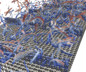
To obtain general ideas for turbulence structures of the present simulations, figure 6 shows examples of images for the instantaneous spanwise vorticity $\omega _z^+$ distributions. Clearly, the flow image for case S1 at $w/k\simeq 1$ is very different from the other images, and its distribution patterns look quite symmetrical over the rib-top region in the $X$–$y$ plane. At $w/k\simeq 1$ as the permeability increases, the concentration of strong vortices near the ribs becomes relaxed, and the vorticity distribution in the near-rib region tends to be similar to that in the core region for case HP1. As for $w/k\simeq 9$, strong smaller vortices near the ribs look expanded towards the core region depending on the increment of the permeability. These observations imply that turbulence levels near the ribs are large and expanded wider towards the channel centre in the permeable cases at both rib spacings.

Figure 6. Examples of snapshots for instantaneous vorticity $\omega _z^+$ distributions in streamwise–wall-normal planes. In case HP1, the vorticity distribution near the ribs and core flow region look similar. Although we see smaller pointed vortices near the ribs in case S9, vortices near the ribs look expanded towards the core flow region in cases HP1 and HP9. The origin of the streamwise axis $X$ is set at the inlet of the computational box.

For the time-mean statistical flow patterns, figure 7 shows the streamlines for each case. The streamlines are presented by plotting contour lines of the stream functions calculated from spanwise-averaged time-mean velocities. Since the purpose of these plots is to show general flow patterns, the lines are drawn with arbitrary spacings. Obviously, the flow patterns in permeable cases change from those of the impermeable cases depending on the permeability. This trend is consistent with that reported by Okazaki et al. (Reference Okazaki, Takase, Kuwata and Suga2022). At $w/k\simeq 1$, as shown in figures 7(e,g), there is no obvious mean recirculation behind the ribs in cases MP1 and HP1, while it exists clearly in each cavity between the ribs in case LP1. The permeability Reynolds numbers listed in table 2 are $Re_K=2.2$, 5.0 and 7.5 for cases LP1, MP1 and HP1, respectively. This implies that the mean recirculation bubbles between the ribs, which seem to be typical d-type recirculation bubbles isolated from outflows like that in case S1 and those in Cui et al. (Reference Cui, Patel and Lin2003) and Leonardi et al. (Reference Leonardi, Orlandi, Smalley, Djenidi and Antonia2003, Reference Leonardi, Orlandi, Djenidi and Antonia2004), tend to vanish when $Re_K$ becomes larger. (Note that we do not mention small vortices behind ligaments of the Kelvin cells.)

Figure 7. Spanwise averaged time-mean streamlines: (a) case S1, (b) case S9, (c) case LP1, (d) case LP9, (e) case MP1, (f) case MP9, (g) case HP1, (h) case HP9. The lines are drawn with arbitrary spacings.

At $w/k\simeq 9$, in figure 7(d) it is observed that the mean recirculation flow submerges into the porous bottom layer at $4< x/k<9$ in case LP9. Compared with the flow pattern in the impermeable case shown in figure 7(b), the centre position of the recirculation shifts downstream, and the length of the recirculation bubble becomes longer. With the increased permeability the mean recirculation submerges into the porous layer in cases MP9 and HP9, as shown in figures 7(f,h), and we can observe the downward flow underneath the rib, which then goes upwards in between the ribs due to the recirculation inside the porous layer. These recirculation bubbles are exposed to outflows as in case S9 and those seen in the k-type rough wall flows of Cui et al. (Reference Cui, Patel and Lin2003), Leonardi et al. (Reference Leonardi, Orlandi, Smalley, Djenidi and Antonia2003) and Ashrafian et al. (Reference Ashrafian, Andersson and Manhart2004). The observed trends of the flow patterns over the porous layers shown in figures 7(d,f,h) agree well with the experimentally reported trends by Okazaki et al. (Reference Okazaki, Shimizu, Kuwata and Suga2020). The permeability Reynolds numbers listed in table 2 are $Re_K=2.7$, 5.2 and 7.5 for cases LP9, MP9 and HP9, respectively. Hence the blocking effect by the rib that keeps mean recirculation bubbles over the porous layer becomes weak, and the recirculation bubbles tend to vanish as $Re_K$ increases.

4.2. Statistical flow characteristics

First, figure 8 compares the present and experimental data at comparable permeability Reynolds numbers since we consider that $Re_K$ is a measure to characterize the present flow trends as discussed in the later sections. The presented profiles in figures 8(a,c) are the streamwise–spanwise plane-averaged time-mean streamwise velocities (for simplicity hereafter, mean velocities)

(4.1)\begin{equation} {\langle U \rangle}=\epsilon{\left\langle U \right\rangle}^{f}=\frac{\epsilon}{S^f}\int_{S^f}\bar{u} \,{\rm d}s, \end{equation}

normalized by the bulk mean velocity $U_b$, that is,

(4.2)\begin{equation} U_b=\frac{1}{H}\int_{-k}^{H-k} {\langle U \rangle}\,{\rm d} y, \end{equation}

where $S$ is an $x$–$z$ plane area, $\epsilon$ is the fluid-phase ratio of the plane area, $\overline {(\cdot )}$ denotes a time-mean variable, and $(\cdot )^f$ denotes a fluid-phase variable. A fluid-phase plane-averaged value of $\phi$ is denoted as ${\left \langle \phi \right \rangle }^{f}$, and a superficially plane-averaged value of $\phi$ is ${\langle \phi \rangle }$, hereafter. The relation between those variables is ${\langle \phi \rangle }=\epsilon {\left \langle \phi \right \rangle }^{f}$. Figures 8(b,d) indicate the plane-averaged root mean square (r.m.s.) velocities, where $u'_i=u_i-\bar {u}_i$, with $(u_1, u_2, u_3)=(u, v, w)$. Although the compared cases are representative, the shown agreement confirms that the present simulation data are useful to elucidate the turbulent flow physics which governs the rib-roughened porous wall flows studied experimentally by Okazaki et al. (Reference Okazaki, Takase, Kuwata and Suga2022).

Figure 8. Comparison with the experimental data of mean velocity and r.m.s. velocities: (a,b) $w/k\simeq 9$ at $Re_K\simeq 5$; (c,d) $w/k\simeq 1$ at $Re_K\simeq 8$. Experimental data are from Okazaki et al. (Reference Okazaki, Takase, Kuwata and Suga2022). The experimental porous media nos 13 and 20 were metallic foam media with porosity $\varphi =0.95$.

Figure 9 compares the simulated mean velocity profiles. It is seen that the mean velocity increases below the rib-top position ($y<0$) as the permeability increases for both $w/k\simeq 1$ and 9. Because of this increase of the flow rate at $y<0$, the velocity profile reduces above the rib-top region while it recovers in the upper half-region. These observed trends are consistent with those shown in the experiments by Okazaki et al. (Reference Okazaki, Takase, Kuwata and Suga2022). As for the velocity magnitudes at the rib-bottom position $y/H=-0.1$, they are very minor even at $w/k\simeq 9$ in case HP. This contrasts with the existence of substantial slip velocities at flat porous interfaces. Indeed, Suga et al. (Reference Suga, Matsumura, Ashitaka, Tominaga and Kaneda2010) and Efstathiou & Luhar (Reference Efstathiou and Luhar2018) reported that at ‘flat’ porous interfaces, there existed substantial slip velocities that were approximately 30 % of the bulk or free-stream velocity. (Interestingly, the velocity magnitudes at the rib-top position $y=0$ are, however, close to those slip velocities.) Accordingly, although flow penetration into the porous layer at $y/H<-0.1$ is observed in permeable cases, it looks very small both at $w/k\simeq 1$ and 9. This indicates that although streamlines are drawn inside the porous bed in figure 7, the flow rate there is negligibly small.

Figure 9. Comparison of plane-averaged time-mean velocities: (a) streamwise mean velocities at $w/k\simeq 1$; (b) streamwise mean velocities at $w/k\simeq 9$.

The profiles of the plane-averaged Reynolds shear stress (for simplicity, Reynolds shear stress hereafter) and dispersion shear stress are shown in figure 10. Here, the velocity dispersion is $\bar {\tilde {u}}_i =\bar {u}_i-{\left \langle \bar {u}_i \right \rangle }^{f}$, and the dispersion stress is defined as

(4.3)\begin{equation} {\langle \bar{\tilde{u}}_i \bar{\tilde{u}}_j \rangle}=\frac{\epsilon}{S^f}\int_{S^f} \left(\bar{u}_i-{\left\langle \bar{u}_i \right\rangle}^{f}\right)\left(\bar{u}_j-{\left\langle \bar{u}_j \right\rangle}^{f}\right){\rm d}s. \end{equation}

At $w/k\simeq 1$, as the permeability increases, the Reynolds shear stress around the rib increases monotonically as shown in figure 10(a). This implies that turbulence is enhanced as the permeability increases. For $w/k\simeq 9$, shown in figure 10(b), such a trend is seen only in the region near the rib-bottom. At the rib-top position, the Reynolds shear stress of case S9 is predominant over the other cases, while the profiles of the permeable cases look almost collapsed to a single profile. This suggests that the turbulence level over the rib at $w/k\simeq 9$ is rather insensitive to the present permeable cases once normalized by the friction velocity. Moreover, the levels of cases HP1 and HP9 over the ribs become almost the same, and this suggests that the rib spacing becomes ineffective to affect turbulence over the ribs at a higher permeability case. As indicated in figure 9(a), in case S1, the magnitude of ${\langle U \rangle }/U_b$ between the ribs is close to zero, though there are locally negative velocities due to the recirculation bubbles as seen in figure 7(a). Correspondingly, $-{\langle \bar {\tilde {u}} \bar {\tilde {v}} \rangle }^+$ shows a negative profile below the rib-top. As the permeability increases, however, such negative local velocities tend to disappear. Similar things take place just over the ribs in case S9. Accordingly, as the permeability increases, the dispersion shear stress changes its sign near the rib, as seen in figures 10(c,d). The penetration of the shear stress is observed until $y/H\simeq -0.3$ in case HP9, unlike in the mean velocity profile. As for the dispersion stress, although its maximum magnitude is 10–20 % of that of the Reynolds shear stress, its levels inside the porous layer at $y/H<-0.1$ become comparable or even larger than those of the Reynolds shear stress for permeable cases MP9 and HP9, as seen in figure 10(d). These trends suggest that surface mass transfer at $y/H<-0.1$ by turbulence and dispersion clearly increases as the increase of the permeability at $w/k\simeq 9$.

Figure 10. Comparison of plane-averaged Reynolds shear and dispersion shear stresses: (a) Reynolds shear stresses at $w/k\simeq 1$; (b) Reynolds shear stresses at $w/k\simeq 9$; (c) dispersion stresses at $w/k\simeq 1$; (d) dispersion stresses at $w/k\simeq 9$.

Figures 11 and 12 indicate the simulated r.m.s. velocities and r.m.s. dispersion velocities, respectively. At $w/k\simeq 1$, the trends of the r.m.s. streamwise velocities over the rib-top position shown in figure 11(a) look different from those in the Reynolds shear stress profiles, while the other components shown in figures 11(c,e) behave similarly to the Reynolds shear stress. The streamwise component of case S1 is larger than in the other cases just above the rib, while the wall-normal and spanwise components of case S1 are smaller than in the other cases. This means that turbulence anisotropy there in case S1 is higher than that in the other cases. Turbulence anisotropy over the rib hence reduces clearly in permeable cases since the permeability weakens turbulence anisotropy near the porous interface (Breugem et al. Reference Breugem, Boersma and Uittenbogaard2006; Suga et al. Reference Suga, Matsumura, Ashitaka, Tominaga and Kaneda2010). At $w/k\simeq 9$, although there are slight discrepancies between the cases, the general trends of the cases look similar to one another. These trends over the rib are also observed in Okazaki et al. (Reference Okazaki, Shimizu, Kuwata and Suga2020). The penetration depths of permeable cases are similar to each other for $w/k\simeq 1$ and $9$ unlike in the Reynolds shear stress profiles, and the permeability enhances the r.m.s. velocities inside the porous layer at $y/H < -0.1$. This implies that inside the porous layer, the wall-normal fluctuating energy induced by the vertical pressure fluctuation is redistributed to the other components. The r.m.s. dispersion velocities inside the porous layer at $y/H<-0.1$ shown in figure 12 at $w/k\simeq 9$ are clearly larger than those at $w/k\simeq 1$, unlike the r.m.s. velocities. This trend corresponds to the mean streamlines presented in figure 7. Particularly at $w/k\simeq 9$, since the mean recirculating flow with certain magnitudes of local velocities exists inside the porous layer, the r.m.s. dispersion velocities exist. While the magnitudes of the r.m.s. dispersion velocities inside the porous layer at $w/k\simeq 9$ tend to be large in the larger permeable cases, those in cases MP9 and HP9 look similar to each other. Such a trend is also seen in the dispersion stress shown in figure 10(d). (Although there seem to be several reasons why this happens, such as the porosity and thickness of the porous layer, we do not discuss this issue further since our main focus is on the flow physics over porous rib roughness. Note that as confirmed in Appendix B, the presently applied porous layer thicknesses are enough to discuss turbulence over porous rib roughness keeping it free from the effects of the very bottom wall.) The trends observed above suggest that mass flux across the porous surface towards the inside region would be significantly larger at $w/k\simeq 9$ than at $w/k\simeq 1$, owing to the dispersion rather than turbulence.

Figure 11. Comparison of plane-averaged r.m.s. velocities: (a) streamwise r.m.s. velocities at $w/k\simeq 1$; (b) streamwise r.m.s. velocities at $w/k\simeq 9$; (c) wall-normal r.m.s. velocities at $w/k\simeq 1$; (d) wall-normal r.m.s. velocities at $w/k\simeq 9$; (e) spanwise r.m.s. velocities at $w/k\simeq 1$; (f) spanwise r.m.s. velocities at $w/k\simeq 9$.

Figure 12. Comparison of r.m.s. dispersion velocities: (a) streamwise components at $w/k\simeq 1$; (b) streamwise components at $w/k\simeq 9$; (c) wall-normal components at $w/k\simeq 1$; (d) wall-normal components at $w/k\simeq 9$; (e) spanwise components at $w/k\simeq 1$; (f) spanwise components at $w/k\simeq 9$.

4.3. Drag characteristics

Corresponding to the trend of turbulence quantities observed in figures 10 and 11, the drag shows characteristic behaviours as seen in figure 13(a) that compares the data with the experiments of Okazaki et al. (Reference Okazaki, Takase, Kuwata and Suga2022). The rib-bottom drag coefficient $C_D$ corresponds to the sum of the frictional and pressure drag coefficients described by Leonardi et al. (Reference Leonardi, Orlandi, Smalley, Djenidi and Antonia2003), who simulated solid impermeable cases, and their data are also included in figure 13(a). In the present study, the definition is $C_D=2\tau _b/(\rho U_b^2)$, where the drag over the rib-bottom $\tau _b$ is calculated by

(4.4)\begin{equation} \tau_b=\left(H-\int_{-k}^0(1-\epsilon)\,{\rm d} y\right)\frac{\Delta p}{L_x}-\tau_t, \end{equation}

since the joint integration of $\tau _b$ and the wall shear stress on the top smooth wall $\tau _t$ balances with the integration of the pressure drop over the rib-bottom. The area over which the pressure drop is integrated is proportional to $H$ minus the streamwise–spanwise plane-averaged solid-phase part of the rib height: $\int _{-k}^0(1-\epsilon )\,{\rm d}y$. Hence $C_D$ here does not include the drag by the porous bottom layer below the rib-bottom, but it includes the pressure and frictional drag through the ribs. It is seen that $C_D$ values of the impermeable cases are in close agreement at $w/k\simeq$1 and 9, while some Reynolds number effects may exist at $w/k\simeq 9$. In both the present and experimental studies, as the permeability (and thus $Re_K$) increases, $C_D$ increases at $w/k\simeq$1, although the reverse trend is seen at $w/k\simeq 9$, while the differences are small between the present permeable cases. These observed trends correspond qualitatively to the changes of the permeability Reynolds number. In figure 13(b), however, we understand that the correlation between $C_D$ and $Re_K$ is not general when experimental data are cross-plotted. Note that the experimental values shown in figures 13(b,c) are somewhat dispersed, particularly at the low $Re_K$ region. As reported in the experiments for flat porous beds by Suga et al. (Reference Suga, Matsumura, Ashitaka, Tominaga and Kaneda2010) and Suga, Mori & Kaneda (Reference Suga, Mori and Kaneda2011), the slippage velocity at the porous interface and the near-wall characteristics of permeable wall turbulence change drastically in the low $Re_K$ region, particularly below $Re_K\simeq 3$. Because of this, the data of Suga et al. (Reference Suga, Matsumura, Ashitaka, Tominaga and Kaneda2010) were scattered, though the general trend looked obvious. Accordingly, the measured values of Okazaki et al. (Reference Okazaki, Takase, Kuwata and Suga2022) look dispersed in the low $Re_K$ region. Such a trend looks somehow exaggerated at $w/k=1$. As $Re_K$ becomes large, there exist asymptotic limiting values of $C_D$ that are independent of $Re_K$ but dependent on the rib spacing. To exclude explicit effects of the pressure drag from the discussion, in figure 13(c) we plot the distributions of $C_f$, which is presently defined as $C_f=2\tau _*/(\rho U_b^2)$. Since the general trends shown in figure 13(c) are the same as those shown in figure 13(b), it is clear that the effects of rib spacing affect the flows over the ribs dynamically. To understand further how the rib-bottom drag is characterized from a phenomenological viewpoint, $C_D$ is next decomposed as in Fukagata, Iwamoto & Kasagi (Reference Fukagata, Iwamoto and Kasagi2002).

Figure 13. Comparison of the rib-bottom drag coefficients. (a) Plots of $C_D$ against the variation of $w/k$; experimental results are at $Re_b\simeq 5000$ from Okazaki et al. (Reference Okazaki, Takase, Kuwata and Suga2022). The permeabilities of nos 13, 20 and 30 metallic foam media are $K/k^2=3.67\times 10^{-3}$, $K/k^2=1.44\times 10^{-3}$ and $K/k^2=7.78\times 10^{-4}$, respectively, while their porosity is $\varphi =0.95$. The DNS data of the impermeable case by Leonardi et al. (Reference Leonardi, Orlandi, Smalley, Djenidi and Antonia2003) are at $Re_b\simeq 7000$. (b) Plots of $C_D$ against the variation of $Re_K$; skin friction coefficient $C_f$ at the porous surface is used for the flat bed cases. Each broken curve is an approximate curve for each rib spacing. (c) Plots of $C_f$ against the variation of $Re_K$; here, $C_f$ is defined as $C_f=2\tau _*/(\rho U_b^2)$.

The $x$–$z$ plane-averaged time-mean momentum equation for the present flows may be written as

(4.5)\begin{equation} 0=-\frac{\epsilon}{\rho}\,\frac{\partial \langle\,\bar{p}\rangle^f}{\partial x}+\frac{\partial}{\partial y}\left(\nu\,\frac{\epsilon \langle\bar{u}\rangle^f}{\partial y}\right) -{\bar{f}_1} -\frac{\partial}{\partial y}(R_{12}+T_{12}), \end{equation}

where $\bar {f}_1$, $R_{12}$ and $T_{12}$ are the drag force, Reynolds stress and dispersion stress terms, respectively. By integrating (4.5) three times, with the equivalent boundary layer thickness $\delta _p=\tau _*(H-k)/(\tau _*+\tau _t)$, the rib-bottom drag coefficient may be decomposed as

(4.6)\begin{align} C_D& =\underbrace{ \frac{ \varPsi}{ Re_b}}_{\text{laminar}} \underbrace{{}-\frac{\varPsi}{2 U_b^2H^2}\int_{-k}^{0}(y+k)(y+k-2H)\bar{f}_1 \,{\rm d} y}_{\text{rib drag}} \nonumber\\ &\quad \underbrace{{}-\frac{\varPsi}{ U_b^2H^2} \int_{-k}^{H-k}(H-k-y)R_{12}\,{\rm d} y}_{\text{turbulence}} \underbrace{{}-\frac{\varPsi}{ U_b^2H^2} \int_{-k}^{H-k}(H-k-y) T_{12}\,{\rm d} y}_{\text{dispersion}}, \end{align}

where $\varPsi$ is calculated as

(4.7)\begin{equation} \varPsi=\left\{ \frac{1}{4}-\frac{\int_{-k}^{0}(H-k-y)^2\epsilon\,{\rm d} y+(H-k)^3/3}{4H^2\left( \int_{-k}^{0}\epsilon\,{\rm d} y+\delta_p \right)}\right\}^{-1}, \end{equation}

since $\epsilon =1$ at $y>0$. The derivation process of (4.6) and (4.7) is detailed in Appendix C. Figure 14 shows the breakdown chart of the rib-bottom drag coefficient. At both $w/k\simeq 1$ and 9, the laminar part, which is $\varPsi /Re_b$ in (4.6), does not change visibly in the simulated cases since $\varPsi$ does not change very much. Indeed, $\varPsi =6.9\unicode{x2013}7.4$ in the range $\delta _p/H=0.4\unicode{x2013}0.7$. The other parts, however, change depending on the permeability and the rib spacing. At $w/k\simeq 1$, the increment of the turbulence part looks sensitive to the increase of the permeability, while the rib-drag part does not look so sensitive. Indeed, although the rib-drag part is slightly larger in the permeable cases, its behaviour is not monotonic. The pressure drag and the skin friction inside the ribs, which compose the rib drag, change depending on the permeability. The former decreases owing to the permeability, while the latter increases as the flow rate through the ribs, as implied in figure 7. The dispersion part is not significant owing to the dispersion shear stress, which is not significant compared with the Reynolds shear stress, as shown in figure 10. Accordingly, the main factor of the increase of $C_D$ at $w/k\simeq 1$ depending on the permeability is the turbulence part.

Figure 14. Breakdown of the rib-bottom drag coefficient. (a) Factors for $w/k\simeq 1$: S1 (laminar $1.49 \times 10^{-3}$, turbulence $7.03 \times 10^{-3}$, dispersion $-3.90 \times 10^{-5}$, rib drag $5.98 \times 10^{-3}$); LP1 (laminar $1.37 \times 10^{-3}$, turbulence $1.59 \times 10^{-2}$, dispersion $3.54 \times 10^{-4}$, rib drag $8.31 \times 10^{-3}$); MP1 (laminar $1.29 \times 10^{-3}$, turbulence $2.28 \times 10^{-2}$, dispersion $9.35 \times 10^{-4}$, rib drag $8.31 \times 10^{-3}$); HP1 (laminar $1.33 \times 10^{-3}$, turbulence $2.95 \times 10^{-2}$, dispersion $9.67 \times 10^{-4}$, rib drag $8.80 \times 10^{-3}$). (b) Factors for $w/k\simeq 9$: S9 (laminar $1.20 \times 10^{-3}$, turbulence $4.28 \times 10^{-2}$, dispersion $2.42 \times 10^{-3}$, rib drag $9.71 \times 10^{-3}$); LP9 (laminar $1.28 \times 10^{-3}$, turbulence $3.16 \times 10^{-2}$, dispersion $1.13 \times 10^{-3}$, rib drag $6.70 \times 10^{-3}$); MP9 (laminar $1.28 \times 10^{-3}$, turbulence $2.90 \times 10^{-2}$, dispersion $1.51 \times 10^{-3}$, rib drag $5.85 \times 10^{-3}$); HP9 (laminar $1.27 \times 10^{-3}$, turbulence $2.95 \times 10^{-2}$, dispersion $1.47 \times 10^{-3}$, rib drag $4.28 \times 10^{-3}$).

At $w/k\simeq 9$, the rib-drag part clearly decreases depending on the permeability. This suggests that the decrease of the pressure drag depending on the permeability is more significant than the increase of the skin friction. The dispersion part becomes larger than that at $w/k\simeq 1$, while its behaviour does not seem to relate to the permeability. As at $w/k\simeq 1$, the turbulence part is most dominant and determines the general trend of $C_D$. Interestingly, the magnitudes of the turbulence parts in cases HP1, LP9, MP9 and HP9 are at the same level. This implies that the turbulence structure may be similar in those cases. Note that the experiments by Suga et al. (Reference Suga, Matsumura, Ashitaka, Tominaga and Kaneda2010) for the ribless flat cases, in which the rib-drag and dispersion parts do not appear, reported much less surface friction, as shown in figure 13(b). This suggests that when we gradually increase the rib spacing to $w/k \rightarrow \infty$, the magnitudes of the turbulence part and rib-bottom drag decrease gradually towards certain levels depending on $Re_K$.

To understand the mutual dependency between the breakdown factors shown in figure 14, we consider the budget equations of the dispersion and Reynolds stresses appearing in (4.5). Following Kuwata & Suga (Reference Kuwata and Suga2013, Reference Kuwata and Suga2015) and Kuwata, Suga & Sakurai (Reference Kuwata, Suga and Sakurai2014), by the double (time and plane) averaging theory (Whitaker Reference Whitaker1996), the budget equations of the dispersion and Reynolds stresses are derived as below. For $\left \langle \bar {\tilde {u}}_i\bar {\tilde {u_j}} \right \rangle ^f$, which corresponds to $T_{ij}/\epsilon$,

(4.8) \begin{align} 0 &= \underbrace{\frac{\partial}{\partial x_k}\left(\nu\,\frac{\partial \left\langle \bar{\tilde{u}}_i \bar{\tilde{u}}_j \right\rangle^f }{\partial x_k}\right)}_{\text{viscous diffusion}} -\underbrace{2\nu \left\langle \frac{\partial \bar{\tilde{u}}_i}{\partial x_k}\,\frac{\partial \bar{\tilde{u}}_j}{\partial x_k}\right\rangle^f}_{\text{viscous dissipation: }\mathcal{E}_{ij}} \underbrace{{}+\bar{f}_i\left\langle \bar{u}_j\right\rangle^f+\bar{f}_j\left\langle \bar{u}_i\right\rangle^f} _{\text{drag force: } \mathcal{F}_{ij}} \nonumber\\ &\quad \underbrace{{}-\frac{\partial}{\partial x_k} \left( \left\langle \bar{\tilde{u}}_j\,\overline{\left\langle u_k' \right\rangle^f\tilde{u}_j'}\right\rangle^f + \left\langle \bar{\tilde{u}}_i\,\overline{\left\langle u_k' \right\rangle^f\tilde{u}_i'}\right\rangle^f + \left\langle \bar{\tilde{u}}_j\, \overline{\tilde{u_k}'\tilde{u}'}_i\right\rangle^f + \left\langle \bar{\tilde{u}}_i\, \overline{\tilde{u_k}'\tilde{u}'}_j\right\rangle^f \right)}_{\text{turbulent diffusion}}\nonumber\\ & \quad \underbrace{{}- \frac{\partial}{\partial x_k} \left( \left\langle \bar{\tilde{u}}_i \bar{\tilde{u}}_j\bar{\tilde{u}}_k\right\rangle^f \right) }_{\text{dispersive diffusion}} \underbrace{{}-\frac{1}{\rho}\left( \frac{\partial \left\langle \bar{\tilde{u}}_i\bar{\tilde{p}}\right\rangle^f}{\partial x_j} +\frac{\partial \left\langle \bar{\tilde{u}}_j\bar{\tilde{p}}\right\rangle^f}{\partial x_i}\right) +\left\langle\frac{\bar{\tilde{p}}}{\rho}\left(\frac{\partial \bar{\tilde{u}}_i}{\partial x_j}+\frac{\partial\bar{\tilde{u}}_j}{\partial x_i}\right)\right\rangle^f}_{\text{pressure correlation: }\mathcal{\varPi}^d_{ij} }\nonumber\\ &\quad \underbrace{{}-\left\langle \bar{\tilde{u}}_i\bar{\tilde{u_k}} \right\rangle^f \frac{\partial \left\langle \bar{u}_j \right\rangle^f}{\partial x_k} -\left\langle \bar{\tilde{u}}_j\bar{\tilde{u_k}} \right\rangle^f \frac{\partial \left\langle \bar{u}_i \right\rangle^f}{\partial x_k}}_{\text{mean shear production: } \mathcal{P}_{ij}} \underbrace{{}- \overline{\left\langle \bar{\tilde{u}}_i \tilde{u}'_k \right\rangle^f \frac{\partial \left\langle u_j' \right\rangle^f}{\partial x_k}} - \overline{\left\langle \bar{\tilde{u}}_j \tilde{u}'_k \right\rangle^f \frac{\partial \left\langle u_i' \right\rangle^f}{\partial x_k}} }_{\text{turbulent shear production: }\mathcal{P}^t_{ij}}\nonumber\\ & \quad \underbrace{{}+ \left\langle \left(\overline{\tilde{u}'_i\tilde{u}'_k}+\overline{\tilde{u}'_i\left\langle u_k' \right\rangle^f}\right) \frac{\partial \tilde{\bar{u}}_j}{\partial x_k} \right\rangle^f + \left\langle \left(\overline{\tilde{u}'_j\tilde{u}'_k}+\overline{\tilde{u}'_j\left\langle u_k' \right\rangle^f}\right) \frac{\partial \tilde{\bar{u}}_i}{\partial x_k} \right\rangle^f}_{\text{counterpart of }P^d_{ij}\text{ in Reynolds stress}}, \end{align}

while for $\langle \overline {u'_i u'_j}\rangle ^f$, which corresponds to $R_{ij}/\epsilon$,

(4.9)\begin{align} 0&= \underbrace{\frac{\partial }{\partial x_k} \left( \nu\,\frac{\partial \langle \overline{u'_i u'_j}\rangle^f }{\partial x_k} \right)}_{\text{viscous diffusion}} -\underbrace{ 2 \nu\left( \overline{\frac{\partial {\left\langle u'_i \right\rangle}^{f}}{\partial x_k}\,\frac{\partial {\left\langle u'_j \right\rangle}^{f}}{\partial x_k}} + \overline{{\left\langle \frac{\partial \tilde{u}'_i}{\partial x_k}\,\frac{\partial \tilde{u}'_j}{\partial x_k} \right\rangle}^{f}}\right)}_{\text{viscous dissipation: }\varepsilon_{ij }}\nonumber\\ &\quad \underbrace{{}-\frac{\partial}{\partial x_k} \left( \overline{{\left\langle u_i' \right\rangle}^{f}{\left\langle u_j' \right\rangle}^{f}{\left\langle u_k' \right\rangle}^{f}}+\overline{{\left\langle \tilde{u}_i'\tilde{u}_j'\tilde{u}_k' \right\rangle}^{f}} \right)}_{\text{turbulent diffusion}} \nonumber\\ & \quad -\frac{\partial}{\partial x_k}\left( \overline{{\left\langle u'_i \right\rangle}^{f}{\left\langle \tilde{u}'_j\tilde{u}'_k \right\rangle}^{f}}+\overline{{\left\langle u'_j \right\rangle}^{f}{\left\langle \tilde{u}'_i\tilde{u}'_k \right\rangle}^{f}} +\overline{{\left\langle u'_i \right\rangle}^{f}{\left\langle \tilde{u}'_j\tilde{\bar{u}}_k \right\rangle}^{f}}+\overline{{\left\langle u'_j \right\rangle}^{f}{\left\langle \tilde{u}'_i\tilde{\bar{u}}_k \right\rangle}^{f}} \right. \nonumber\\ & \qquad \underbrace{ \left.{}+\overline{{\left\langle u'_i \right\rangle}^{f}{\left\langle \tilde{\bar{u}}_j\tilde{u}'_k \right\rangle}^{f}}+\overline{{\left\langle u'_j \right\rangle}^{f}{\left\langle \tilde{\bar{u}}_i\tilde{u}'_k \right\rangle}^{f}} +\overline{{\left\langle u'_k \right\rangle}^{f}{\left\langle \tilde{u}'_i\tilde{u}'_j \right\rangle}^{f}}+\overline{{\left\langle \tilde{\bar{u}}_k\tilde{u}'_i\tilde{u}'_j \right\rangle}^{f}} \right)}_{\text{dispersive diffusion}} \nonumber\\ & \quad \underbrace{{}-\frac{1}{\rho}\left( \overline{{\left\langle u'_j \right\rangle}^{f}\frac{\partial {\left\langle \,p' \right\rangle}^{f} }{\partial x_i}} +\overline{{\left\langle u'_i \right\rangle}^{f}\frac{\partial {\left\langle \,p' \right\rangle}^{f} }{\partial x_j}} +\overline{{\left\langle \tilde{u}'_i\,\frac{\partial \tilde{p}'}{\partial x_j} \right\rangle}^{f} } +\overline{{\left\langle \tilde{u}'_j\, \frac{\partial \tilde{p}'}{\partial x_i} \right\rangle}^{f} } \right)}_{\text{pressure correlation: }\varPi_{ij}}\nonumber\\ & \quad \underbrace{{}-\langle \overline{u'_i u'_k}\rangle^f\frac{\partial {\left\langle \bar{u}_j \right\rangle}^{f}}{\partial x_k} -\langle \overline{u'_j u'_k}\rangle^f\frac{\partial {\left\langle \bar{u}_i \right\rangle}^{f}}{\partial x_k}}_{\text{mean shear production: }P_{ij}} \underbrace{+\overline{{\left\langle \tilde{u}'_k \tilde{\bar{u}}_i \right\rangle}^{f}\frac{\partial {\left\langle u'_j \right\rangle}^{f}}{\partial x_k}}+\overline{{\left\langle \tilde{u}'_k \tilde{\bar{u}}_j \right\rangle}^{f}\frac{\partial {\left\langle u'_i \right\rangle}^{f}}{\partial x_k}}}_{\text{counterpart of }\mathcal{P}^t_{ij}{\text{ in dispersion stress}}} \nonumber\\ & \quad \underbrace{{}-{\left\langle \left(\overline{\tilde{u}'_i\tilde{u}'_k} +\overline{\tilde{u}'_i{\left\langle u'_k \right\rangle}^{f}} \right)\frac{\partial \tilde{\bar{u}}_j}{\partial x_k} \right\rangle}^{f} -{\left\langle \left(\overline{\tilde{u}'_j\tilde{u}'_k} +\overline{\tilde{u}'_j{\left\langle u'_k \right\rangle}^{f}} \right)\frac{\partial \tilde{\bar{u}}_i}{\partial x_k} \right\rangle}^{f}}_{\text{dispersive shear production: }P^d_{ij}}. \end{align}

When the mean shear $\partial \langle \bar {u}_1\rangle /\partial x_2$ exists, from the budget ((4.8) and (4.9)), the mutual energy transfer cycle between the mean flow, dispersion and turbulence fields may be illustrated as in figure 15. Since only the momentum and dispersion stress equations ((4.5) and (4.8)) include the drag force terms, $\mathcal {F}_{11}=2\bar {f}_1{\left \langle \bar {u} \right \rangle }^{f}$ in the budget equation of $T_{11}$ solely feeds direct effects of the drag force to the dispersion field, while the turbulence field does not receive any direct contribution from the drag force. Since the enhanced energy of $T_{11}$ is redistributed to the other components by the pressure correlation, the energy gained by $\mathcal {F}_{11}$ is redistributed to $T_{22}$ through $\varPi ^d_{22}$. Then by $\mathcal {P}_{12}$ with the mean shear, $T_{12}$ is enhanced. The enhanced $T_{12}$ increases $T_{11}$ by $\mathcal {P}_{11}$, and so on. By the dispersive shear production $P^d_{ij}$ (called ‘wake production’ in canopy flows; Finnigan Reference Finnigan2000), the dispersion field feeds energy to the turbulence field, while some energy back-scatter from the turbulence field by $\mathcal {P}^t_{ij}$ exists. The diffusion terms spatially diffuse each stress, and $\mathcal {E}_{ij}$ dissipates some of the kinetic energy. Accordingly, since the drag force has direct relations to the projection area of the roughness elements, the roughness effects on turbulence come through the mean shear and the energy transfer from the dispersion field by $P^d_{ij}$. As for the mutual energy transfer cycle in the turbulence field, it is achieved by the same manner as in the dispersion field.

Figure 15. Conceptual illustration of energy flows between mean flow, dispersion and turbulence fields under mean shear. The mean flow field feeds the mean shear $\partial \langle \bar {u}_1\rangle /\partial x_2$ to the dispersion and turbulence fields. The drag force effect is given only to $T_{11}$ through $\mathcal {F}_{11}$. The dispersion and turbulence fields exchange their energy by $P^d_{ij}$ and $\mathcal {P}^t_{ij}$. The dispersion and Reynolds shear stresses ($T_{12}$, $R_{12}$) feed back to the mean flow field through the momentum equation. The mean shear production terms ($\mathcal {P}_{ij}$, $P_{ij}$) are the main sources of the stresses, while the wall-normal components $T_{22}$ and $R_{22}$ do not have the mean shear production. The pressure correlation terms ($\varPi ^d_{ij}$, $\varPi _{ij}$) redistribute energy to the other components ($T_{33}$ and $R_{33}$ are not shown). Although they are not illustrated, the dissipation and diffusion processes exist.

In case S1, since figure 9(a) implies that the velocity gradient in the rib region $-0.1< y/H<0$ is rather small, the drag force contribution through the mean velocity seems small. Indeed, the corresponding magnitude of the Reynolds shear stress in $-0.1< y/H<0$ is very small, as shown in figure 10(a). Moreover in figure 14, the (integrated) dispersion part in case S1 is invisibly small. Note that since the dispersion in the region over the rib-top reflects the skewed streamlines caused by the rib roughness as seen in figure 7, the integrated dispersion includes rib effects not only in the rib region but also in the region above the ribs. This suggests that the rib-roughness effects are merely transferred to the turbulence part of case S1, while the rib-bottom drag includes roughness effects by the rib-drag part, which is not so small. The above consideration is consistent with the fact that turbulence at $w/k=1$ in the solid case is not characterized by the roughness scale and categorized in the d-type roughness. In the other cases, however, as seen in figures 9 and 14, the mean shear and the dispersion part have certain levels, while they seem quite small in case LP1. Accordingly, the turbulence parts in the permeable cases should have certain effects of roughness scales via the mean shear and dispersion fields. (See figure 10 for the increase of the Reynolds shear stress at $y<0$ depending on the permeability.) This discussion supports the recent studies of Lee & Sung (Reference Lee and Sung2007), MacDonald et al. (Reference MacDonald, Ooi, García-Mayoral, Hutchins and Chung2018) and Xu et al. (Reference Xu, Altland, Yang and Kunz2021), which reported that non-k-type roughness was not automatically classified as the d-type roughness. Hence the increment of the dispersion part as the permeability at $w/k\simeq 1$ in figure 14 correlates to the transition from the d-type roughness to the k-type roughness. The above energy flow mechanism also explains why the studies by Stoyanova et al. (Reference Stoyanova, Wang, Sekimoto, Okano and Takagi2019), Kim et al. (Reference Kim, Blois and Christensen2020) and Shen et al. (Reference Shen, Yuan and Phanikumar2020) showed that the dispersion played a significant role in modifying turbulence.

4.4. Characteristic roughness height

To see the region up to where the roughness effects extend, figure 16 compares the streamwise r.m.s. velocity profiles. The smooth wall channel flow profiles at $Re_\tau =395$ (Moser, Kim & Mansour Reference Moser, Kim and Mansour1999) and 550 (Hoyas & Jiménez Reference Hoyas and Jiménez2008) are also compared. In any case, the difference between the present and smooth channel cases becomes evident in the regions $y/\delta _p < 0.6$ and 0.3 for $w/k\simeq 1$ and 9, respectively. It is hence confirmed that the roughness effects extend up to those distances, which correspond approximately to $y=4k$ and $2k$, respectively.

Figure 16. Streamwise r.m.s. velocity profiles against the wall-normal distance normalized by $\delta _p$: (a) at $w/k\simeq 1$, (b) at $w/k\simeq 9$. The smooth wall channel data at $Re_\tau =395$ and 550 are from Moser et al. (Reference Moser, Kim and Mansour1999) and Hoyas & Jiménez (Reference Hoyas and Jiménez2008), respectively.

For the mean velocity profiles, we apply the logarithmic formula by Best (Reference Best1935):

(4.10)\begin{equation} \frac{{\langle U \rangle}}{u_*}=\kappa^{-1}\ln \frac{y+d_0}{h_0}, \end{equation}

where $d_0$ and $h_0$ are the zero-plane displacement and a roughness scale. Usually, this has been applied to the flows over porous media and canopies (Nikora et al. Reference Nikora, Koll, McLean, Dittrich and Aberle2002; Breugem et al. Reference Breugem, Boersma and Uittenbogaard2006; Nepf & Ghisalberti Reference Nepf and Ghisalberti2008; Suga et al. Reference Suga, Matsumura, Ashitaka, Tominaga and Kaneda2010; Manes et al. Reference Manes, Poggi and Ridol2011). Using the fitting method described well in the literature (e.g. Breugem et al. Reference Breugem, Boersma and Uittenbogaard2006; Okazaki et al. Reference Okazaki, Takase, Kuwata and Suga2022), the profiles are fitted to (4.10) for obtaining $\kappa$, $d_0$ and $h_0$, which are listed in table 2. Figures 17(a,b) show the presently fitted mean velocity profiles. Although there would be arguments against logarithmic fitting for relatively low Reynolds number flows, as shown in figures 17(c,d), the log-law indicator $\beta =(y+d_0)^+ \partial {\langle U \rangle }^+/\partial y^+$ profiles show reasonably flat regions except for case S1. (For case LP, although the iteration number is reasonably large for obtaining the turbulence statistics, the plots suggest that it is not large enough for $\beta$. Hence we admit that the values for case LP obtained by the fitting contain certain errors.) We thus recognize that the flows in the present permeable cases have reasonable logarithmic velocity regions, except for case S1 in which a flat profile of $\beta$ is not confirmed. Accordingly, we define the region below the log layer as the ‘nominal’ roughness sublayer, with its thickness $\delta _r$ as indicated graphically in figure 17(c). It is the distance between the zero-plane and the point where the $\beta$ profile matches the horizontal flat line. Table 2 also lists the values of $\delta _r$ normalized by $u_*$. The nominal roughness sublayer thickness does not correspond to the thickness discussed with figure 16. In fact, $(\delta _r-d_0)/\delta _p= 0.03\unicode{x2013}0.11$. Moreover, when the zero-plane is considered for the origin of the boundary layer, the ratio of the nominal roughness sublayer to the boundary layer thickness is $\delta _r/(\delta _p+d_0)=0.13\unicode{x2013}0.26$ in the present cases.

Figure 17. Streamwise plane-averaged mean velocity distributions in the semi-log scale and log-law indicator functions: (a) mean velocity profiles at $w/k\simeq 1$; (b) mean velocity profiles at $w/k\simeq 9$; (c) log-law indicator function $\beta$ at $w/k\simeq 1$, with the graphical definition of the nominal roughness sublayer thickness $\delta _r$; (d) log-law indicator function $\beta$ at $w/k\simeq 9$. The solid thin horizontal lines in (c,d) correspond to $\beta =1/\kappa$.

In permeable wall turbulence, $\kappa$ is no longer constant, depending on the permeability as reported by Breugem et al. (Reference Breugem, Boersma and Uittenbogaard2006), Suga et al. (Reference Suga, Matsumura, Ashitaka, Tominaga and Kaneda2010) and Manes et al. (Reference Manes, Poggi and Ridol2011). Indeed, for $Re_b>90\,000$, Manes et al. (Reference Manes, Poggi and Ridol2011) fitted their data with $\kappa =0.32$. As shown in figure 18, although the experimental values of Okazaki et al. (Reference Okazaki, Takase, Kuwata and Suga2022) show a somewhat scattered distribution, the plots distribute around the present results and one can see a general trend of $\kappa$ depending on $Re_K$. Interestingly, although there may be $w/k$ sensitivity, it looks less sensitive to $w/k$ than the rib-bottom drag coefficient discussed with figure 13.

Figure 18. Variation of the von Kármán constant versus the permeability Reynolds number.

Another logarithmic formula of Nikuradse (Reference Nikuradse1933) is, however, applied widely to discuss wall roughness. With the equivalent sand-grain roughness height $k_s$, it reads

(4.11)\begin{equation} \frac{{\langle U \rangle}}{u_*}=\kappa^{-1}\ln \frac{\hat{y}}{k_s}+8.5, \end{equation}

where $\hat {y}$ is the wall-normal distance from the origin, which should be determined empirically (Jiménez Reference Jiménez2004). Accordingly, in this study $\hat {y}=y+d_0$ is applied. (The scaling of $d_0$ was discussed extensively by Okazaki et al. (Reference Okazaki, Takase, Kuwata and Suga2022). They reported that although $d_0$ depended on both the rib spacing and the permeability, once the zero-plane displacement for the corresponding impermeable case $d_s$ was given, $(d_0-d_s)^+$ was scaled as $(d_0-d_s)^+\simeq 14 Re_K$ or $(d_0-d_s)^+\simeq D^+_p$, where $D_p^+$ was the pore Reynolds number.) By coupling (4.10) and (4.11), we can re-fit the velocity data to Nikuradse's formula, and $k_s$ can be rewritten with $h_0$ as $k_s=h_0\exp (8.5\kappa ).$ However, we think that this process to estimate $k_s$ is not a legitimately acceptable way to determine the equivalent sand-grain roughness height. We then call such a value the ‘characteristic roughness height’:

(4.12)\begin{equation} k^*_s=h_0\exp(8.5\kappa), \end{equation}

hereafter. Table 2 lists the obtained $k^*_s$ normalized by $u_*$, and indicates that all cases are in the ‘nominally’ fully rough regime of $k_s^{*+}>70$, except for case S1. Although the roughness function may be discussed, it is unsure how to determine the log-law shifts in this study due to the variation of the slant angle of the semi-logarithmic velocity profile, as seen in figure 17. Accordingly, this study focuses on $k^*_s$ as a parameter for roughness effects. Note that although $h_0$ is another candidate for the parameter, since $k^*_s$ includes explicitly the effects of $h_0$ and the non-constant $\kappa$ by (4.12), we have found that $k^*_s$ is a better scale to characterize permeable roughness, as discussed below.

Initially, we considered that $\delta _p$ might be a candidate to scale $k^*_s$ at a higher $Re_K$ since reasonable distributions of $k^*_s/\delta _p$ were seen in the present data. We have, however, found that it is not true by conducting an additional simulation of an open channel flow whose height corresponds to $\delta _p/k=10$ for case MP9. This additional case is named MP9-OC, hereafter. The results indicate that since $Re_\tau$ is set to the same as that of case MP9, the obtained parameters do not change significantly from those of case MP9, although $k^*_s/\delta _p$ changes significantly. The parameters of case MP9-OC are $\kappa =0.26$, $d_0^+=95$, $h_0^+=38$, $ks^{*+}=346$ and $\delta _r^+=128$. They change slightly from the original values of case MP9 listed in table 2. Note that since the values of the parameters including the changing $\kappa$ are slightly affected by $\delta _p/k$ (and hence $H/k$), the results indicate a certain limitation of the set-up adopted in this study.

Instead of $\delta _p$, to discuss the permeability effect on $k^*_s$, we have found that the nominal roughness sublayer thickness $\delta _r$ is better than the viscous length scale for scaling $k^*_s$, as shown in figure 19. Indeed, we see that including the above additional result of case MP9-OC, $k^*_s$ maintains a close relation with an inner layer parameter $\delta _r$. It is seen that when $Re_K$ becomes larger, asymptotically $k^*_s/\delta _r$ reaches approximately 2.5 for both $w/k\simeq 1$ and 9. Since the levels and characteristics of turbulence become quite similar in cases LP9, MP9, HP9 and HP1, we consider that the values of $k^*_s/\delta _r$ in those cases become similar. Experiments by Okazaki et al. (Reference Okazaki, Takase, Kuwata and Suga2022) support this trend for the higher $Re_K$ cases, as seen in figure 19. When $w/k$ becomes larger, as also indicated in figure 19, the experimental data by Okazaki et al. (Reference Okazaki, Takase, Kuwata and Suga2022) for $w/k=19$ and the flat porous bed cases by Suga et al. (Reference Suga, Matsumura, Ashitaka, Tominaga and Kaneda2010) also distribute around $k^*_s/\delta _r\simeq 2.5$ at $Re_K>7$. Hence at a higher $Re_K$ that is larger than 7, $k^*_s/\delta _r$ becomes independent of $Re_K$ and looks almost constant around $2.5$ irrespective of the rib spacing, while in the transitional stage at $Re_K<7$, $k^*_s/\delta _r$ varies depending on the cases. These trends suggest that some of the turbulence characteristics become insensitive to the surface topology at a high permeability Reynolds number. This is supported by the discussion of Voermans et al. (Reference Voermans, Ghisalberti and Ivey2017), who reported that many turbulence characteristics became independent of $Re_K$ as it increased. White & Nepf (Reference White and Nepf2007) also reported that the details of the porous layer were not important for the vortex structure once the inner layer instability was established.

Figure 19. Characteristic roughness height versus the permeability Reynolds number. The star symbol is from the additional simulation with a higher channel height. The thin black dashed line indicates $k^*_s/\delta _r=2.5$.

4.5. Premultiplied energy spectra

To see the turbulence structures from spectrum spaces, figure 20 describes the one-dimensional premultiplied streamwise energy spectrum $(E_{uu, x}\kappa _x)^+$ distributions in the wall-normal direction. As for $w/k\simeq 1$, although the most energetic region is detached from the rib-top position at $y=0$ in case S1, the levels of the energetic regions become lower, and the most energetic points look attached on the rib-top position ($y=0$) in permeable cases. This corresponds to the profiles shown in figure 11(a). It is also seen that the energy with larger wavelengths propagates more toward the edge of the boundary layer, and the shapes of the contours tend to be square-like ones as the permeability increases. Notably, the most energetic wavelength in each case becomes slightly larger as the permeability increases. In case HP1, it becomes $\lambda _x/\delta _p\simeq 2$. As for $w/k\simeq 9$, the trends for the energy propagation and the most energetic wavelength are also observed, while in case HP9, the most energetic wavelength $\lambda _x$ looks a little larger than $2\delta _p$. Furthermore, the outermost contours of cases HP1 and HP9 resemble each other, suggesting that some turbulence structures tend to be similar irrespective of the rib spacing when the permeability Reynolds number is high. This corresponds to the trends discussed in § 4.4 with figure 19.

Figure 20. Premultiplied energy spectral distributions in the $y$-direction. The contours of $(E_{uu, x}\kappa _x)^+$ are plotted in the $\lambda _x/\delta _p$–$y/\delta _p$ plane. The parameters $\kappa _x$ and $\lambda _x$ are the wavenumber and wavelength in the streamwise direction, respectively. The overlaid black lines in (a,c,e) and (b,d,f) are for cases S1 and S9, respectively. Plots are for (a) case LP1, (b) case LP9, (c) case MP1, (d) case MP9, (e) case HP1, (f) case HP9.

Figure 21 shows two-dimensional premultiplied energy spectra $(E_{uu, xz}\kappa _x\kappa _z)^+$ for the $x$–$z$ planes at $y/k=0.5$. In the permeable cases, for both $w/k\simeq 1$ and 9, the most energetic point of $(E_{uu, xz}\kappa _x\kappa _z)^+$ is almost fixed at $\lambda _x/\delta _p\simeq 2$ in the streamwise direction, while in the region $\lambda _x/\delta _p > 2$, the contours tend to shift upwards in the spanwise direction as the permeability increases. This trend implies that some structures are expanded in the spanwise direction depending on the increase of the permeability, although it is not a clear evidence of the existence of spanwise rollers. Indeed, the roller structure cannot be confirmed in the two-point streamwise correlations shown in figure 5(a). Although the study by Kuwata & Suga (Reference Kuwata and Suga2016b) on turbulence over a flat porous bed observed spanwise rollers even at a relatively low $Re_K=3.8$, once the surfaces are roughened, it may be considered that strong perturbations arising from the roughness elements disturb the development of such a structure. Spanwise rollers generated by the Kelvin–Helmholtz instability owing to velocity inflection may be appearing at much larger Reynolds numbers for the present flow configurations.

Figure 21. Two-dimensional premultiplied energy spectra for the streamwise–spanwise planes at $y/k=0.5$. The contours of $(E_{uu, x}\kappa _x)^+$ are plotted in the $\lambda _x/\delta _p$–$\lambda _z/\delta _p$ plane. The overlaid black lines in (a,c,e) and (b,d,f) are for cases S1 and S9, respectively. Plots are for (a) case LP1, (b) case LP9, (c) case MP1, (d) case MP9, (e) case HP1, (f) case HP9.