


1 Introduction
Surface gravity waves are an important route by which the ocean exchanges energy, momentum, heat and gases with the overlying atmosphere (Cavaleri, Fox-Kemper & Hemer Reference Cavaleri, Fox-Kemper and Hemer2012; Villas Bôas et al. Reference Villas Bôas2019). Sea-surface currents modify the wavenumber, direction and amplitude of surface waves, and affect the spatial variability of the wave field. The effect of currents on waves under the Wentzel–Kramers–Brillouin (WKB) approximation has been well studied (Kenyon Reference Kenyon1971; Peregrine Reference Peregrine1976; White & Fornberg Reference White and Fornberg1998; Henderson et al. Reference Henderson, Guza, Elgar and Herbers2006; Heller, Kaplan & Dahlen Reference Heller, Kaplan and Dahlen2008; Gallet & Young Reference Gallet and Young2014). But the sparseness of ocean current observations makes it difficult to explicitly account for wave–current interactions in numerical surface-wave models. Thus, instead of explicit resolving sea-surface currents, a statistical approach to the effect of currents on surface waves is required.
Recent studies of surface wave–current interactions suggest that the sea-state variability at meso- and submesoscales, here referred to as macroturbulence, is dominated by the variability of the current field (Ardhuin et al. Reference Ardhuin, Gille, Menemenlis, Rocha, Rascle, Chapron, Gula and Molemaker2017; Quilfen et al. Reference Quilfen, Yurovskaya, Chapron and Ardhuin2018; Quilfen & Chapron Reference Quilfen and Chapron2019). At these scales, horizontally divergent motions associated with tides, inertia-gravity waves, and fronts contribute significantly to the surface kinetic energy (Bühler, Callies & Ferrari Reference Bühler, Callies and Ferrari2014; Rocha et al. Reference Rocha, Chereskin, Gille and Menemenlis2016a; D’Asaro et al. Reference D’Asaro, Shcherbina, Klymak, Molemaker, Novelli, Guigand, Haza, Haus, Ryan and Jacobs2018). If surface gravity waves respond differently to divergent than to rotational flows – and we show here that they do – then changes in the dominant regime of surface currents can result in significant changes in the surface-wave field. This offers the possibility that observations of surface gravity waves might be used to probe the structure of submesoscale ocean turbulence.
In the context of internal gravity waves, McComas & Bretherton (Reference McComas and Bretherton1977) showed how scale-separated wave interactions can be analysed with the WKB approximation and understood as diffusion of wave action. The induced diffusion approximation of McComas and Bretherton has recently been developed and extended by Kafiabad, Savva & Vanneste (2019, KSV, hereafter) to obtain an action-diffusion equation for the scattering of internal gravity waves by mesoscale ocean turbulence. Here we apply the KSV method to surface gravity waves. Crucial to this development is that the parameter
 $$\begin{eqnarray}\unicode[STIX]{x1D716}\stackrel{\text{def}}{=}|\boldsymbol{U}|/c\end{eqnarray}$$
 is small; above,  $\boldsymbol{U}$ is the horizontal current at the sea surface and $c=\sqrt{g/4k}$ is the deep-water group speed at wavenumber $k$.
$k$.
In § 2, and in appendix A, we use the formalism of KSV to derive an expression for a diffusivity tensor of surface-wave action. In § 3 we consider the simplifications that result from assuming that the sea-surface velocity  $\boldsymbol{U}$ has isotropic statistics. We show that the horizontally divergent component of $\boldsymbol{U}$ has no effect on action diffusivity: diffusivity results solely from the vortical (solenoidal) component of $\boldsymbol{U}$ and produces an angular diffusivity that is expressed as a weighted integral of the solenoidal part of the energy spectrum of $\boldsymbol{U}$ as in (3.20). Smit & Janssen (Reference Smit and Janssen2019) have also examined the action diffusion of surface waves using a framework based on Lagrangian random walk theory. Section 3 discusses the differences between Smit and Janssen’s expression for the action diffusivity and ours. In § 4 the analytic results are tested with Monte Carlo ray tracing through an ensemble of stochastic velocity fields.
2 The induced diffusion approximation
For linear deep-water surface waves, the Doppler-shifted dispersion relation is
 $$\begin{eqnarray}\unicode[STIX]{x1D714}(t,\boldsymbol{x},\boldsymbol{k})=\unicode[STIX]{x1D70E}+\boldsymbol{k}\boldsymbol{\cdot }\boldsymbol{U}(t,\boldsymbol{x}),\end{eqnarray}$$
 where  $\boldsymbol{k}=(k_{1},k_{2})$ is the wavenumber, $\unicode[STIX]{x1D70E}=\sqrt{gk}$ is the intrinsic wave frequency, with $k=|\boldsymbol{k}|$ and $g$ the gravitational acceleration. Also in (2.1), $\boldsymbol{U}(t,\boldsymbol{x})=(U_{1},U_{2})$ is the horizontal current at the sea surface. Provided that $\boldsymbol{U}(t,\boldsymbol{x})$ is slowly varying with respect to the waves (i.e. the temporal scales of variations in the current field are longer and the spatial scales are larger than those of the waves), wave kinematics is described by the ray equations. Using index notation the ray equations are
 $$\begin{eqnarray}{\dot{x}}_{n}=\unicode[STIX]{x2202}_{k_{n}}\unicode[STIX]{x1D714}=c_{n}+U_{n}\quad \text{and}\quad \dot{k}_{n}=-\unicode[STIX]{x2202}_{x_{n}}\unicode[STIX]{x1D714}=-U_{m,n}k_{m},\end{eqnarray}$$
 where  $c_{n}=\unicode[STIX]{x2202}_{k_{n}}\unicode[STIX]{x1D70E}(k)$ is the group velocity. Under the same assumptions, wave dynamics is governed by the conservation of wave action density $A(\boldsymbol{x},\boldsymbol{k},t)$
 $$\begin{eqnarray}\unicode[STIX]{x2202}_{t}A+{\dot{x}}_{n}\unicode[STIX]{x2202}_{x_{n}}A+\dot{k}_{n}\unicode[STIX]{x2202}_{k_{n}}A=0,\end{eqnarray}$$
 with  ${\dot{x}}_{n}$ and $\dot{k}_{n}$ given by (2.2) (Phillips Reference Phillips1966; Mei Reference Mei1989).
We follow KSV and develop a multiple-scale solution, based on  $\unicode[STIX]{x1D716}\ll 1$, that enables one to average (2.3) over the ensemble of velocity fields $\boldsymbol{U}$ (see appendix A). Assuming that the statistical properties of $\boldsymbol{U}$ are stationary and homogeneous, one finds that
 $$\begin{eqnarray}\unicode[STIX]{x2202}_{t}\bar{A}+c_{n}\unicode[STIX]{x2202}_{x_{n}}\bar{A}=\unicode[STIX]{x2202}_{k_{j}}\unicode[STIX]{x1D60B}_{jn}\unicode[STIX]{x2202}_{k_{n}}\!\bar{A},\end{eqnarray}$$
 where  $\bar{A}$ denotes the ensemble average of $A$. The diffusivity tensor $\unicode[STIX]{x1D60B}_{jn}$ in (2.4) is expressed in terms of the two-point velocity correlation tensor
 $$\begin{eqnarray}\unicode[STIX]{x1D61D}_{im}(\boldsymbol{x}-\boldsymbol{x}^{\prime })\stackrel{\text{def}}{=}\langle U_{i}(\boldsymbol{x})U_{m}(\boldsymbol{x}^{\prime })\rangle .\end{eqnarray}$$
 Because of the assumption of spatial homogeneity,  $\unicode[STIX]{x1D61D}_{im}$ depends only on the separation $\boldsymbol{r}=\boldsymbol{x}-\boldsymbol{x}^{\prime }$ of the two points. The most convenient formula for explicit calculation of $\unicode[STIX]{x1D60B}_{jn}$ is the Fourier space result
 $$\begin{eqnarray}\unicode[STIX]{x1D60B}_{jn}=\frac{k_{i}k_{m}k}{4\unicode[STIX]{x03C0}c}\int q_{j}q_{n}\tilde{\unicode[STIX]{x1D61D}}_{im}(\boldsymbol{q})\unicode[STIX]{x1D6FF}(\boldsymbol{q}\boldsymbol{\cdot }\boldsymbol{k})\,\text{d}\boldsymbol{q},\end{eqnarray}$$
 where  $c=g/2\unicode[STIX]{x1D70E}$ is the magnitude of the group velocity and
 $$\begin{eqnarray}\tilde{\unicode[STIX]{x1D61D}}_{im}(\boldsymbol{q})=\int \text{e}^{-\text{i}\boldsymbol{r}\boldsymbol{\cdot }\boldsymbol{q}}\unicode[STIX]{x1D61D}_{im}(\boldsymbol{r})\,\text{d}\boldsymbol{r}\end{eqnarray}$$
 is the Fourier transform of  $\unicode[STIX]{x1D61D}_{im}(\boldsymbol{r})$. (In (2.6) and (2.7) the integrals cover the entire two-dimensional planes $(q_{1},q_{2})$ and $(r_{1},r_{2})$ respectively.) The diffusivity in (2.6) is the two-dimensional equivalent of (A7) in KSV. Our appendix A derivation, however, assumes only spatial homogeneity and stationarity of the velocity $\boldsymbol{U}$, and does not require incompressibility of $\boldsymbol{U}$.
One can verify from (2.6) that  $\unicode[STIX]{x1D60B}_{jn}k_{n}=0$ and therefore there is no diffusion of wave action in the radial direction in $\boldsymbol{k}$-space. Fast surface-wave packets propagate through a frozen field of macroturbulent eddies and thus preserve the absolute frequency $\sqrt{gk}+\boldsymbol{U}\boldsymbol{\cdot }\boldsymbol{k}$. Because $\unicode[STIX]{x1D716}$ in (1.1) is small, the Doppler shift $\boldsymbol{U}\boldsymbol{\cdot }\boldsymbol{k}$ is small relative to the intrinsic frequency $\sqrt{gk}$. Thus, at leading order, both $\unicode[STIX]{x1D70E}$ and $k$, are constant. In other words, absolute frequency conservation, together with $\unicode[STIX]{x1D716}\ll 1$, implies that there is no radial $\boldsymbol{k}$-diffusion in (2.4). Thus, scattering by weak surface currents results mainly in directional diffusion of surface gravity waves.
3 Diffusion of wave action density by isotropic velocity fields
The derivation of (2.6) makes essential use of the assumption that the spatial statistics of  $\boldsymbol{U}$ are spatially homogeneous. We now make the further assumption that the statistical properties of $\boldsymbol{U}$ are also isotropic and investigate the contributions of vertical vorticity and horizontal divergence to $\unicode[STIX]{x1D60B}_{jn}$. We follow Bühler et al. (Reference Bühler, Callies and Ferrari2014) and represent $\boldsymbol{U}$ with a two-dimensional Helmholtz decomposition into rotational (solenoidal) and irrotational (potential) components
 $$\begin{eqnarray}\boldsymbol{U}=(U,V)=(\unicode[STIX]{x1D719}_{x}-\unicode[STIX]{x1D713}_{y},\unicode[STIX]{x1D719}_{y}+\unicode[STIX]{x1D713}_{x}).\end{eqnarray}$$
 The streamfunction  $\unicode[STIX]{x1D713}$ and velocity potential $\unicode[STIX]{x1D719}$ have the two-point correlation functions
 $$\begin{eqnarray}C^{\unicode[STIX]{x1D713}}(r)=\langle \unicode[STIX]{x1D713}(\boldsymbol{x})\unicode[STIX]{x1D713}(\boldsymbol{x}^{\prime })\rangle \quad \text{and}\quad C^{\unicode[STIX]{x1D719}}(r)=\langle \unicode[STIX]{x1D719}(\boldsymbol{x})\unicode[STIX]{x1D719}(\boldsymbol{x}^{\prime })\rangle .\end{eqnarray}$$
 If the velocity ensemble is not mirror invariant under reflection with respect to an axis in the  $(x,y)$-plane, then there might also be a ‘cross-correlation’ between $\unicode[STIX]{x1D713}$ and $\unicode[STIX]{x1D719}$:
 $$\begin{eqnarray}C^{\unicode[STIX]{x1D713}\unicode[STIX]{x1D719}}(r)\stackrel{\text{def}}{=}\langle \unicode[STIX]{x1D713}(\boldsymbol{x})\unicode[STIX]{x1D719}(\boldsymbol{x}^{\prime })\rangle =\langle \unicode[STIX]{x1D713}(\boldsymbol{x}^{\prime })\unicode[STIX]{x1D719}(\boldsymbol{x})\rangle .\end{eqnarray}$$
 Because of isotropy, the scalar correlation functions introduced in (3.2) and (3.3) depend only on the distance  $r=|\boldsymbol{r}|$ between points $\boldsymbol{x}$ and $\boldsymbol{x}^{\prime }$. Therefore, $\unicode[STIX]{x2202}_{r_{i}}=\unicode[STIX]{x2202}_{x_{i}}=-\unicode[STIX]{x2202}_{x_{i}^{\prime }}$. Using the notation $\boldsymbol{r}=(r_{1},r_{2})$, the $\unicode[STIX]{x1D61D}_{11}$ component of the velocity autocorrelation tensor in (2.5) can be expressed in terms of the scalar correlation functions as
 $$\begin{eqnarray}\displaystyle \unicode[STIX]{x1D61D}_{11}(\boldsymbol{r}) & = & \displaystyle \langle U(\boldsymbol{x})U(\boldsymbol{x}^{\prime })\rangle ,\end{eqnarray}$$
 $$\begin{eqnarray}\displaystyle & = & \displaystyle \langle \unicode[STIX]{x1D713}_{y}\unicode[STIX]{x1D713}_{y^{\prime }}\rangle -\langle \unicode[STIX]{x1D713}_{y^{\prime }}\unicode[STIX]{x1D719}_{x}\rangle -\langle \unicode[STIX]{x1D713}_{y}\unicode[STIX]{x1D719}_{x^{\prime }}\rangle +\langle \unicode[STIX]{x1D719}_{x}\unicode[STIX]{x1D719}_{x^{\prime }}\rangle ,\end{eqnarray}$$
 $$\begin{eqnarray}\displaystyle & = & \displaystyle -\unicode[STIX]{x2202}_{r_{2}}^{2}C^{\unicode[STIX]{x1D713}}+2\unicode[STIX]{x2202}_{r_{1}}\unicode[STIX]{x2202}_{r_{2}}C^{\unicode[STIX]{x1D713}\unicode[STIX]{x1D719}}-\unicode[STIX]{x2202}_{r_{1}}^{2}C^{\unicode[STIX]{x1D719}}.\end{eqnarray}$$
 Similar calculations for the other components of  $\unicode[STIX]{x1D61D}_{im}$ result in
 $$\begin{eqnarray}\unicode[STIX]{x1D61D}_{im}=\unicode[STIX]{x1D61D}_{im}^{\unicode[STIX]{x1D713}}+\unicode[STIX]{x1D61D}_{im}^{\unicode[STIX]{x1D713}\unicode[STIX]{x1D719}}+\unicode[STIX]{x1D61D}_{im}^{\unicode[STIX]{x1D719}},\end{eqnarray}$$
with
 $$\begin{eqnarray}\unicode[STIX]{x1D61D}_{im}^{\unicode[STIX]{x1D713}}=\left[\begin{array}{@{}cc@{}}-\unicode[STIX]{x2202}_{r_{2}}^{2} & \unicode[STIX]{x2202}_{r_{1}}\unicode[STIX]{x2202}_{r_{2}}\\ \unicode[STIX]{x2202}_{r_{1}}\unicode[STIX]{x2202}_{r_{2}} & -\unicode[STIX]{x2202}_{r_{1}}^{2}\end{array}\right]C^{\unicode[STIX]{x1D713}},\quad \unicode[STIX]{x1D61D}_{im}^{\unicode[STIX]{x1D719}}=-\left[\begin{array}{@{}cc@{}}\unicode[STIX]{x2202}_{r_{1}}^{2} & \unicode[STIX]{x2202}_{r_{1}}\unicode[STIX]{x2202}_{r_{2}}\\ \unicode[STIX]{x2202}_{r_{1}}\unicode[STIX]{x2202}_{r_{2}} & \unicode[STIX]{x2202}_{r_{2}}^{2}\end{array}\right]C^{\unicode[STIX]{x1D719}}\end{eqnarray}$$
and
 $$\begin{eqnarray}\unicode[STIX]{x1D61D}_{im}^{\unicode[STIX]{x1D713}\unicode[STIX]{x1D719}}=\left[\begin{array}{@{}cc@{}}2\unicode[STIX]{x2202}_{r_{1}}\unicode[STIX]{x2202}_{r_{2}} & \unicode[STIX]{x2202}_{r_{2}}^{2}-\unicode[STIX]{x2202}_{r_{1}}^{2}\\ \unicode[STIX]{x2202}_{r_{2}}^{2}-\unicode[STIX]{x2202}_{r_{1}}^{2} & 2\unicode[STIX]{x2202}_{r_{1}}\unicode[STIX]{x2202}_{r_{2}}\end{array}\right]C^{\unicode[STIX]{x1D713}\unicode[STIX]{x1D719}}.\end{eqnarray}$$
 The Fourier transform of (3.8) and (3.9) follows with  $\unicode[STIX]{x2202}_{r_{i}}\mapsto \text{i}q_{i}$ and is equal to
 $$\begin{eqnarray}\tilde{\unicode[STIX]{x1D61D}}_{im}^{\unicode[STIX]{x1D713}}(\boldsymbol{q})=(q^{2}\unicode[STIX]{x1D6FF}_{im}-q_{i}q_{m})\tilde{C}^{\unicode[STIX]{x1D713}}(q),\quad \tilde{\unicode[STIX]{x1D61D}}_{im}^{\unicode[STIX]{x1D719}}(\boldsymbol{r})=q_{i}q_{m}\tilde{C}^{\unicode[STIX]{x1D719}}(q)\end{eqnarray}$$
and
 $$\begin{eqnarray}\tilde{\unicode[STIX]{x1D61D}}_{im}^{\unicode[STIX]{x1D713}\unicode[STIX]{x1D719}}(\boldsymbol{q})=(q_{i}q_{m}^{\bot }+q_{i}^{\bot }q_{m})\tilde{C}^{\unicode[STIX]{x1D713}\unicode[STIX]{x1D719}}(q),\end{eqnarray}$$
 where  $\boldsymbol{q}^{\bot }=(-q_{2},q_{1})$ is the perpendicular vector to $\boldsymbol{q}=(q_{1},q_{2})$. Also in (3.10) and (3.11)
 $$\begin{eqnarray}\tilde{C}^{\unicode[STIX]{x1D713}}(q)=2\unicode[STIX]{x03C0}\int _{0}^{\infty }C^{\unicode[STIX]{x1D713}}(r)\text{J}_{0}(qr)r\,\text{d}r,\end{eqnarray}$$
 with  $\text{J}_{0}$ the Bessel function of order zero, is the Fourier transform of the axisymmetric function $C^{\unicode[STIX]{x1D713}}(r)$. The expressions for $\tilde{C}^{\unicode[STIX]{x1D719}}(q)$ and $\tilde{C}^{\unicode[STIX]{x1D713}\unicode[STIX]{x1D719}}(q)$ are analogous to (3.12).
Substituting (3.10) and (3.11) into (2.6) we have
 $$\begin{eqnarray}k_{i}k_{m}\tilde{\unicode[STIX]{x1D61D}}_{im}(\boldsymbol{q})=k^{2}q^{2}\tilde{C}^{\unicode[STIX]{x1D713}}(q)+\cdots \,,\end{eqnarray}$$
 where  $\cdots \,$ above indicates the three other terms that arise from contracting (3.10) and (3.11) with $k_{i}k_{m}$. Each of these three terms, however, contains a factor $\boldsymbol{k}\boldsymbol{\cdot }\boldsymbol{q}$. Courtesy of $\unicode[STIX]{x1D6FF}(\boldsymbol{k}\boldsymbol{\cdot }\boldsymbol{q})$ in the integrand of (2.6), the $\ldots$ in (3.13) makes no contribution to $\unicode[STIX]{x1D60B}_{jn}$ and the diffusivity tensor reduces to
 $$\begin{eqnarray}\displaystyle \unicode[STIX]{x1D60B}_{jn}(\boldsymbol{k})=\frac{k^{3}}{4\unicode[STIX]{x03C0}c}\int q^{2}q_{j}q_{n}\tilde{C}^{\unicode[STIX]{x1D713}}(q)\unicode[STIX]{x1D6FF}(\boldsymbol{q}\boldsymbol{\cdot }\boldsymbol{k})\,\text{d}\boldsymbol{q}, & & \displaystyle\end{eqnarray}$$
 where the integral covers the entire  $(q_{1},q_{2})$-plane. The diffusion tensor in (3.14) does not depend on the velocity potential $\unicode[STIX]{x1D719}$. Using $\unicode[STIX]{x1D6FF}(\boldsymbol{q}\boldsymbol{\cdot }\boldsymbol{k})$ to evaluate one of the two integrals in (3.14) one obtains
 $$\begin{eqnarray}\unicode[STIX]{x1D60B}_{jn}(\boldsymbol{k})=\frac{1}{2\unicode[STIX]{x03C0}c}\left[\begin{array}{@{}cc@{}}k_{2}^{2} & -k_{1}k_{2}\\ -k_{1}k_{2} & k_{1}^{2}\end{array}\right]\int _{0}^{\infty }q^{4}\tilde{C}^{\unicode[STIX]{x1D713}}(q)\,\text{d}q.\end{eqnarray}$$
 It is remarkable that the compressible and irrotational component of the velocity field, produced by the velocity potential  $\unicode[STIX]{x1D719}$, makes no contribution to the action-diffusion tensor in (3.15). Dysthe (Reference Dysthe2001) shows that in the weak-current limit, $\unicode[STIX]{x1D716}\ll 1$, the ray curvature is equal to $\unicode[STIX]{x1D701}/c$, where $\unicode[STIX]{x1D701}=\unicode[STIX]{x1D713}_{xx}+\unicode[STIX]{x1D713}_{yy}$ is the vertical vorticity of the surface currents; see § 68 of Landau & Lifshitz (Reference Landau and Lifshitz1987) and Gallet & Young (Reference Gallet and Young2014) for alternative derivations. These ray-tracing results rationalize the result in (3.15) that diffusion of surface-wave action by sea-surface currents is produced only by the vortical and horizontally incompressible component of the sea-surface velocity.
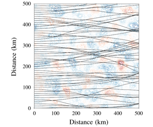
This effect is illustrated in figure 1, where we show ray trajectories obtained by numerical integration of the ray equations (2.2) for waves with a period of 10 s propagating through three different types of surface flows (purely solenoidal, purely potential, and combined solenoidal and potential). These synthetic surface currents were created from a scalar function with random phase and prescribed spectral slope ( $q^{-2.5}$ in this case). In panel (a) this function is used as a streamfunction $\unicode[STIX]{x1D713}$ to generate an incompressible vortical flow. In panel (b) the same function is used as a velocity potential $\unicode[STIX]{x1D719}$ to generate an irrotational horizontally divergent flow. In panels (b) and (e), with pure potential flow, the ray trajectories are close to straight lines (i.e. there is almost no scattering). The flow in panel (c) is constructed by summing the velocity fields in panels (a) and (b). Even though the flow in panel (c) is twice as energetic as that in panel (a), the ray trajectories in panels (d) and (f) are very similar. This is a striking confirmation of (3.14): the diffusivity is not affected by $\unicode[STIX]{x1D719}$.

Figure 1. Illustration of the effects of different surface flow regimes on the diffusion of surface waves. Surface flow fields are shown in (a–c) and the respective ray trajectories in (d–f). Panels (a) and (d) show solenoidal flow; (b,e) potential flow. Panels (c) and (f) show a combination of solenoidal and potential flows (the velocity in (c) is the sum of the velocities in (a) and (b)). The mean kinetic energy of (a) and (b) are equal, whereas (c) has twice that of (a) and (b). All rays are initialized from the left side of the domain at  $x=0$ with direction $\unicode[STIX]{x1D703}=0^{\circ }$ and a period equal to 10 s.
Because  $\unicode[STIX]{x1D60B}_{jn}k_{n}=0$, the diffusive flux of wave action, $-\unicode[STIX]{x1D60B}_{jn}\unicode[STIX]{x2202}_{k_{n}}\bar{A}$, is in the direction of $\boldsymbol{k}^{\bot }=k\hat{\unicode[STIX]{x1D73D}}$, where $(k,\unicode[STIX]{x1D703})$ are polar coordinates in the $\boldsymbol{k}$-plane and $\hat{\unicode[STIX]{x1D73D}}$ is a unit vector in the $\unicode[STIX]{x1D703}$-direction. Using these polar coordinates simplifies the $\unicode[STIX]{x2202}_{k_{j}}$ and $\unicode[STIX]{x2202}_{k_{n}}$ derivatives on the right of (2.4) so that the averaged action equation becomes
 $$\begin{eqnarray}\bar{A}_{t}+c\cos \unicode[STIX]{x1D703}\bar{A}_{x}+c\sin \unicode[STIX]{x1D703}\bar{A}_{y}=\unicode[STIX]{x1D6FC}\bar{A}_{\unicode[STIX]{x1D703}\unicode[STIX]{x1D703}},\end{eqnarray}$$
where
 $$\begin{eqnarray}\unicode[STIX]{x1D6FC}(k)=\frac{1}{2\unicode[STIX]{x03C0}c}\int _{0}^{\infty }q^{4}\tilde{C}^{\unicode[STIX]{x1D713}}(q)\,\text{d}q\end{eqnarray}$$
is the directional diffusivity.
To conclude this section we express  $\unicode[STIX]{x1D6FC}$ in (3.17) in terms of the energy spectrum of the solenoidal component of the velocity $\tilde{E}^{\unicode[STIX]{x1D713}}(q)$, related to $\tilde{C}^{\unicode[STIX]{x1D713}}(q)$ by
 $$\begin{eqnarray}\tilde{E}^{\unicode[STIX]{x1D713}}(q)=\frac{q^{3}}{4\unicode[STIX]{x03C0}}\tilde{C}^{\unicode[STIX]{x1D713}}(q).\end{eqnarray}$$
 The spectrum is normalized so that the root-mean-square velocity of the solenoidal component,  ${\mathcal{U}}_{\unicode[STIX]{x1D713}}$, is
 $$\begin{eqnarray}{\mathcal{U}}_{\unicode[STIX]{x1D713}}^{2}=\langle \unicode[STIX]{x1D713}_{x}^{2}\rangle =\langle \unicode[STIX]{x1D713}_{y}^{2}\rangle ={\textstyle \frac{1}{2}}\langle |\boldsymbol{\unicode[STIX]{x1D6FB}}\unicode[STIX]{x1D713}|^{2}\rangle =\int _{0}^{\infty }\tilde{E}^{\unicode[STIX]{x1D713}}(q)\,\text{d}q.\end{eqnarray}$$
 Then  $\unicode[STIX]{x1D6FC}(k)$ can be written as
 $$\begin{eqnarray}\unicode[STIX]{x1D6FC}(k)=\frac{2}{c}\int _{0}^{\infty }q\tilde{E}^{\unicode[STIX]{x1D713}}(q)\,\text{d}q.\end{eqnarray}$$
Taking the trace of the velocity correlation tensors in (3.10) and (3.11) shows that the total energy spectrum is
 $$\begin{eqnarray}\tilde{E}=\tilde{E}^{\unicode[STIX]{x1D713}}(q)+\tilde{E}^{\unicode[STIX]{x1D719}}(q),\end{eqnarray}$$
 where  $\tilde{E}^{\unicode[STIX]{x1D719}}(q)$ is obtained by $\unicode[STIX]{x1D713}\mapsto \unicode[STIX]{x1D719}$ in (3.19). As anticipated in figure 1, the diffusivity $\unicode[STIX]{x1D6FC}(k)$ in (3.20) depends only on the spectrum of the solenoidal component, $\tilde{E}^{\unicode[STIX]{x1D713}}(q)$.
Smit & Janssen (Reference Smit and Janssen2019) arrive at an expression for  $\unicode[STIX]{x1D6FC}(k)$ differing from (3.20) in two respects: (i) the coefficient in front of the integral on the right is $(1/c)$; and (ii) the integrand is $\tilde{E}(q)$. This expression agrees with (3.20) only for the special class of isotropic velocity fields considered by Smit and Janssen in which the integral of $\tilde{E}^{\unicode[STIX]{x1D719}}(q)$ is equal to the integral of $\tilde{E}^{\unicode[STIX]{x1D713}}(q)$ (i.e. isotropic flows in which kinetic energy is equipartitioned between the solenoidal, $\unicode[STIX]{x1D713}$, and the potential, $\unicode[STIX]{x1D719}$, components). An example of an equipartitioned flow is shown in figure 1(c,f) and discussed further in § 4 (see the $+$ simulations). Equipartition, however, is not characteristic of ocean macroturbulence (for example, large scales are in geostrophic balance and are therefore solenoidal). In this pure solenoidal case the diffusivity in Smit & Janssen (Reference Smit and Janssen2019) would be too small by a factor of two.
4 A numerical example using ray tracing
Equation (3.16) has an exact solution that can be used to test (3.20). Begin by noting that
 $$\begin{eqnarray}\frac{\text{d}}{\text{d}t}\iiint A\,\text{d}x\,\text{d}y\,\text{d}\unicode[STIX]{x1D703}=0,\end{eqnarray}$$
 where the integrals above are over the whole  $(x,y)$-plane and over $-\unicode[STIX]{x03C0}<\unicode[STIX]{x1D703}\leqslant \unicode[STIX]{x03C0}$. This is, of course, conservation of action. Multiplying (3.16) by $\cos \unicode[STIX]{x1D703}$ and integrating over $(x,y,\unicode[STIX]{x1D703})$ one obtains
 $$\begin{eqnarray}\frac{\text{d}}{\text{d}t}\iiint \cos \unicode[STIX]{x1D703}A\,\text{d}x\,\text{d}y\,\text{d}\unicode[STIX]{x1D703}=-\unicode[STIX]{x1D6FC}\iiint \cos \unicode[STIX]{x1D703}\,A\,\text{d}x\,\text{d}y\,\text{d}\unicode[STIX]{x1D703}.\end{eqnarray}$$
Combining the time integrals of (4.1) and (4.2) we find
 $$\begin{eqnarray}\langle \cos \unicode[STIX]{x1D703}\rangle =\langle \cos \unicode[STIX]{x1D703}\rangle _{0}\text{e}^{-\unicode[STIX]{x1D6FC}t},\end{eqnarray}$$
 where  $\langle \rangle$ denotes the action-weighted average and $\langle \cos \unicode[STIX]{x1D703}\rangle _{0}$ is the initial value of $\langle \cos \unicode[STIX]{x1D703}\rangle$. At large times $\langle \cos \unicode[STIX]{x1D703}\rangle \rightarrow 0$ with an e-folding time $\unicode[STIX]{x1D6FC}^{-1}$: this is long-time isotropization of the wave field by eddy scattering. To investigate short-time and small-angle scattering, consider for simplicity an initial condition such as that in figure 1 with initial direction $\unicode[STIX]{x1D703}_{0}=0$. Then with $\unicode[STIX]{x1D6FC}t\ll 1$ and $\unicode[STIX]{x1D703}\ll 1$, it follows from (4.3) that $\langle \unicode[STIX]{x1D703}^{2}\rangle \approx 2\unicode[STIX]{x1D6FC}t$.
To test our result for the diffusivity  $\unicode[STIX]{x1D6FC}$, we verify $\langle \unicode[STIX]{x1D703}^{2}\rangle \approx 2\unicode[STIX]{x1D6FC}t$ by numerical integration of the ray-tracing equations (2.2) for surfaces waves with an initial period of 10 s propagating through an ensemble of stochastic velocity fields. The ensemble is created by assigning random phases to each Fourier component of the stream function $\unicode[STIX]{x1D713}$ and velocity potential $\unicode[STIX]{x1D719}$.

Figure 2. Comparison between the Monte Carlo ray-tracing simulations averaged across an ensemble of stochastic velocity fields (markers) and the analytical result  $\langle \unicode[STIX]{x1D703}^{2}\rangle \approx 2\unicode[STIX]{x1D6FC}t$ (solid lines). Here we show the results for an energy spectrum with spectral slopes following a $q^{-n}$ power law where $n=5/3$, 2, 2.5, or 3. Circles $\circ$ are the result for solenoidal flows; diamonds $\diamond$, for potential flows; and crosses $+$ for the combination of solenoidal and potential. The solenoidal and potential flows have mean square velocity $0.01~\text{m}^{2}~\text{s}^{-2}$, whereas the combined flow $+$ has mean square velocity $0.02~\text{m}^{2}~\text{s}^{-2}$. The initial period and direction of the waves are 10 s and $0^{\circ }$, respectively.
The energy spectrum of the sea-surface velocity is modelled with power laws  $\tilde{E}^{\unicode[STIX]{x1D713}}(q)$ and $\tilde{E}^{\unicode[STIX]{x1D719}}(q)\propto q^{-n}$, with $q_{1}<q<q_{2}$ and no energy outside the interval $(q_{1},q_{2})$. The spectra are normalized with prescribed mean square velocities ${\mathcal{U}}_{\unicode[STIX]{x1D713}}^{2}$ and ${\mathcal{U}}_{\unicode[STIX]{x1D719}}^{2}$ as in (3.19). For $n\neq (1,2)$ the integral in (3.20) is evaluated as:
 $$\begin{eqnarray}\unicode[STIX]{x1D6FC}=\frac{2}{c}\frac{(n-1)}{(n-2)}\frac{(q_{1}^{2-n}-q_{2}^{2-n})}{(q_{1}^{1-n}-q_{2}^{1-n})}{\mathcal{U}}_{\unicode[STIX]{x1D713}}^{2}.\end{eqnarray}$$
 For  $n=1$
$n=1$
 $$\begin{eqnarray}\unicode[STIX]{x1D6FC}=\frac{2}{c}\frac{(q_{2}-q_{1})}{\ln (q_{2}/q_{1})}{\mathcal{U}}_{\unicode[STIX]{x1D713}}^{2}\end{eqnarray}$$
 and for  $n=2$
$n=2$
 $$\begin{eqnarray}\unicode[STIX]{x1D6FC}=\frac{2}{c}\frac{q_{1}q_{2}}{q_{2}-q_{1}}\ln (q_{2}/q_{1}){\mathcal{U}}_{\unicode[STIX]{x1D713}}^{2}.\end{eqnarray}$$
 We take  $q_{1}=2\unicode[STIX]{x03C0}/150~\text{km}$ and $q_{2}=2\unicode[STIX]{x03C0}/1~\text{km}$ and spectral slopes $n=(5/3,2.0,2.5,3.0)$. For each $n$ we consider three cases corresponding to the three columns in figure 1: $\circ$
- ${\mathcal{U}}_{\unicode[STIX]{x1D713}}=0.1~\text{m}~\text{s}^{-1}$ and ${\mathcal{U}}_{\unicode[STIX]{x1D719}}=0$;
- $\diamond$
- ${\mathcal{U}}_{\unicode[STIX]{x1D713}}=0$ and ${\mathcal{U}}_{\unicode[STIX]{x1D719}}=0.1~\text{m}~\text{s}^{-1}$;
- $+$
- ${\mathcal{U}}_{\unicode[STIX]{x1D713}}=0.1~\text{m}~\text{s}^{-1}$ and ${\mathcal{U}}_{\unicode[STIX]{x1D719}}=0.1~\text{m}~\text{s}^{-1}$.


Figure 2 summarizes the results by showing  $\langle \unicode[STIX]{x1D703}^{2}\rangle$ as a function of time obtained by averaging 2000 rays. The results are in agreement with $\langle \unicode[STIX]{x1D703}^{2}\rangle \approx 2\unicode[STIX]{x1D6FC}t$ using $\unicode[STIX]{x1D6FC}$ obtained from (4.4) and (4.6). In particular, there is good agreement between $\langle \unicode[STIX]{x1D703}^{2}\rangle$ for case $\circ$ and the analytic result (solid lines). As expected, the potential component of the velocity has no effect on the diffusion of wave action. Thus, in case $\diamond$ – pure potential flow – there is no diffusion of action. In case $+$ the flow has twice as much kinetic energy (and shear) as in cases $\circ$ and $\diamond$; this is also an example of a flow with kinetic energy equipartitioned between the solenoidal and potential components (Smit & Janssen Reference Smit and Janssen2019). Doubling the strength of the flow, by adding a $\unicode[STIX]{x1D719}$ component, does not significantly increase action diffusion above that of case $\circ$.
At the final time, two days, the  $n=5/3$ simulations shown in figure 2 have $\sqrt{\langle \unicode[STIX]{x1D703}^{2}\rangle }$ of order $30^{\circ }$ and the other, steeper, spectral slopes result in smaller directional spreading. Thus, none of the Monte Carlo simulations shown in figure 2 have lasted long enough to result in isotropization of the wave field. We verified, however, that longer simulations are in agreement with (4.3) when $\unicode[STIX]{x1D6FC}t\sim 1$ (not shown).
We conclude this section by noting that numerical and observational evidence supports the hypothesis that  $\tilde{E}(q)\sim q^{-2}$ on submesoscales (very roughly, scales less than 50 km). Horizontally divergent motions contribute significantly the total surface kinetic energy in this range, but the solenoidal component is not negligible (Rocha et al. Reference Rocha, Gille, Chereskin and Menemenlis2016b; Torres et al. Reference Torres, Klein, Menemenlis, Qiu, Su, Wang, Chen and Fu2018; Kafiabad, Savva & Vanneste Reference Kafiabad, Savva and Vanneste2019; Morrow et al. Reference Morrow2019). There is considerable geographic variation. For example, the Gulf Stream region is an exception, with $\tilde{E}(q)\sim q^{-3}$ and little indication of horizontally divergent motions (Bühler et al. Reference Bühler, Callies and Ferrari2014). These results indicate that spectral slope $-2$ is relevant to oceanic application of (3.20). But with $-2$, the integral on the right of (3.20) is sensitive to high-wavenumber solenoidal energy (i.e. to the value of the high-wavenumber cutoff $q_{2}$), as in (4.6). This problem is worse for spectral slopes shallower than $-2$, and less severe in the Gulf Stream region with the steeper slope $-3$.
$-3$.
In the absence of a high-wavenumber transition to a spectral fall-off steeper than  $-2$, the cutoff $q_{2}$ might be determined by the failure of the WKB approximation once the horizontal scales of $\boldsymbol{U}$ are comparable to the hundred-metre wavelengths of surface gravity waves. These considerations complicate the practical application of (3.20) in some oceanic regimes, and indicate the necessity of better understanding the interaction of surface gravity waves with wave-scale currents.
5 Conclusions
Our expression for the action diffusivity in (2.6) assumes that the WKB approximation is valid and that  $\unicode[STIX]{x1D716}=|\boldsymbol{U}|/c\ll 1$. Typical sea-surface currents are of order $0.1~\text{m}~\text{s}^{-1}$, while the swell band has group velocities that exceed $5~\text{m}~\text{s}^{-1}$. Thus, $\unicode[STIX]{x1D716}\ll 1$ is not restrictive. Our analysis also neglects effects associated with vertical shear of the flow, which would modify the Doppler-shifted dispersion relationship (Kirby & Chen Reference Kirby and Chen1989).
We derived an expression for the diffusivity of surface-wave action in (2.6) and demonstrated that for isotropic surface currents the action diffusivity can be expressed in terms of the kinetic energy spectrum of the flow as in (3.20). This result shows that the potential component makes no contribution to action diffusion. Our results are illustrated both qualitatively (figure 1) and quantitatively (figure 2) by numerical solution of the ray equations. Although the numerical examples presented here were obtained for synthetic flows having random phase, the results are also valid in the presence of coherent structures, such as axisymmetric vortices, as long as the statistics remain isotropic (not shown). To leading order, there is no difference between the diffusivity obtained for rays propagating through a pure solenoidal flow and the same solenoidal flow with the addition of an equally strong potential component. Provided that  $\unicode[STIX]{x1D716}\ll 1$, the horizontally divergent and irrotational component of the sea-surface velocity has no effect on the action diffusion of surface gravity waves.
Recent studies motivated by the upcoming Surface Water and Ocean Topography (SWOT) satellite mission have found that surface kinetic energy spectra in the ocean are marked by a transition scale from balanced geostrophic motions (horizontally non-divergent) to unbalanced horizontally divergent motions such as inertia-gravity waves (for example, Rocha et al. Reference Rocha, Chereskin, Gille and Menemenlis2016a,Reference Rocha, Gille, Chereskin and Menemenlisb; Torres et al. Reference Torres, Klein, Menemenlis, Qiu, Su, Wang, Chen and Fu2018; Qiu et al. Reference Qiu, Chen, Klein, Wang, Torres, Fu and Menemenlis2018; Morrow et al. Reference Morrow2019). At scales shorter than this ‘transition’ scale, the kinetic energy spectrum of the potential component of the currents has been observed to dominate over the solenoidal component. In this regime, only a small fraction of the total kinetic energy of the flow would be contributing to the diffusion of surface-wave action.
Perhaps the most important application of our results is in the realm of operational surface-wave models. Wave models, such as WaveWatch III, solve the action balance equation (2.3) with additional terms to account for wind forcing, nonlinear interactions and wave dissipation (Wavewatch III Development Group 2009). Explicitly solving for wave–current interactions in surface-wave models poses two main challenges: it is computationally costly and surface current observations at scales shorter than 100 km are rare (Ardhuin et al. Reference Ardhuin, Roland, Dumas, Bennis, Sentchev, Forget, Wolf, Girard, Osuna and Benoit2012). The wave action diffusivity calculated here can be easily implemented as an additional term in operational wave models, allowing the effects of the currents to be accounted for based on statistical properties of the sea-surface velocity. Although not discussed in the present manuscript, it is also worth noting that refraction of surface waves by meso- and submesoscale flows will ultimately lead to deviations of the wave propagation from the great-circle route, impacting path lengths and, subsequently, arrival times (Smit & Janssen Reference Smit and Janssen2019). A statistical approach to account for these effects in numerical wave models could potentially improve arrival-time predictions.
Acknowledgements
The authors thank the two anonymous reviewers for their suggestions in improving this manuscript. The authors are also thankful to B. D. Cornuelle, S. T. Gille, M. R. Mazloff, P. B. Smit and J. Vanneste for helpful discussions and suggestions, and G. Castelão for helping with the optimization of the ray-tracing solver. A.B.V.B. was funded by NASA Earth and Space Science Fellowship award no. 80NSSC17K0326 and by NASA award NNX16AH67G. W.R.Y. is supported by the National Science Foundation Award OCE-1657041.
Declaration of interests
The authors report no conflict of interest.
Appendix A. The induced diffusion approximation
In this appendix we reprise the KSV multiscale derivation of the induced diffusion approximation showing that the KSV assumption that  $\boldsymbol{U}$ is incompressible is not necessary. All that is required is spatial homogeneity of the statistical properties of the sea-surface velocity $\boldsymbol{U}$.
We follow KSV and introduce the small parameter  $\unicode[STIX]{x1D716}$ defined in (1.1) into the conservation equation of wave action (2.3) by writing $U_{m}\mapsto \unicode[STIX]{x1D716}U_{m}$. With slow space and time scales $\boldsymbol{X}=\unicode[STIX]{x1D716}^{2}\boldsymbol{x}$ and $T=\unicode[STIX]{x1D716}^{2}t$, the action equation (2.3) becomes
 $$\begin{eqnarray}\unicode[STIX]{x2202}_{t}A+c_{n}\unicode[STIX]{x2202}_{x_{n}}A+\unicode[STIX]{x1D716}^{2}\unicode[STIX]{x2202}_{T}A+\unicode[STIX]{x1D716}^{2}c_{n}\unicode[STIX]{x2202}_{X_{n}}A+\unicode[STIX]{x1D716}U_{n}\unicode[STIX]{x2202}_{x_{n}}A+\unicode[STIX]{x1D716}^{3}U_{n}\unicode[STIX]{x2202}_{X_{n}}A-\unicode[STIX]{x1D716}k_{m}U_{m,n}\unicode[STIX]{x2202}_{k_{n}}A=0.\end{eqnarray}$$
 With the expansion  $A=A_{0}(\boldsymbol{X},\boldsymbol{k},T)+\unicode[STIX]{x1D716}A_{1}(\boldsymbol{x},\boldsymbol{X},\boldsymbol{k},t,T)+\cdots \,$ we satisfy the leading-order equation. Then, at order $\unicode[STIX]{x1D716}^{1}$:
 $$\begin{eqnarray}\unicode[STIX]{x2202}_{t}A_{1}+c_{n}\unicode[STIX]{x2202}_{x_{n}}A_{1}=k_{m}U_{m,n}\unicode[STIX]{x2202}_{k_{n}}A_{0},\end{eqnarray}$$
with solution
 $$\begin{eqnarray}A_{1}=k_{m}\int _{0}^{t}U_{m,n}(\boldsymbol{x}-\unicode[STIX]{x1D70F}\boldsymbol{c})\,\text{d}\unicode[STIX]{x1D70F}\unicode[STIX]{x2202}_{k_{n}}A_{0}.\end{eqnarray}$$
 At order  $\unicode[STIX]{x1D716}^{2}$ the problem is
 $$\begin{eqnarray}\unicode[STIX]{x2202}_{t}A_{2}+c_{n}\unicode[STIX]{x2202}_{x_{n}}A_{2}+\unicode[STIX]{x2202}_{T}A_{0}+c_{n}\unicode[STIX]{x2202}_{X_{n}}A_{0}=k_{i}U_{i,j}(\boldsymbol{x})\unicode[STIX]{x2202}_{k_{j}}A_{1}-U_{i}(\boldsymbol{x})\unicode[STIX]{x2202}_{x_{i}}A_{1}.\end{eqnarray}$$
 Pulling out  $\unicode[STIX]{x2202}_{k_{j}}$ from the first term on the right of (A 4) and recombining we obtain
 $$\begin{eqnarray}\unicode[STIX]{x2202}_{t}A_{2}+c_{n}\unicode[STIX]{x2202}_{x_{n}}A_{2}+\unicode[STIX]{x2202}_{T}A_{0}+c_{n}\unicode[STIX]{x2202}_{X_{n}}A_{0}=\unicode[STIX]{x2202}_{k_{j}}k_{i}U_{i,j}(\boldsymbol{x})A_{1}-\unicode[STIX]{x2202}_{x_{i}}(U_{i}(\boldsymbol{x})A_{1}).\end{eqnarray}$$
 None of these manipulations require  $U_{i,i}=0$. Assuming spatial homogeneity and taking the average over an ensemble of velocity fields, here denoted by an overbar, the last term on the right of (A 5) is the fast- $x$ derivative of an average, which is zero because of spatial homogeneity. In the limit of $t\rightarrow \infty$, and using the expression for $A_{1}$ in (A 3), we find
 $$\begin{eqnarray}\unicode[STIX]{x2202}_{T}\bar{A}+c_{n}\unicode[STIX]{x2202}_{X_{n}}\bar{A}=\unicode[STIX]{x2202}_{k_{j}}\unicode[STIX]{x1D60B}_{jn}\unicode[STIX]{x2202}_{k_{n}}\bar{A},\end{eqnarray}$$
 where  $\bar{A}$ is the ensemble average of $A_{0}$ and
 $$\begin{eqnarray}\unicode[STIX]{x1D60B}_{jn}(\boldsymbol{k})=k_{i}k_{m}\int _{0}^{\infty }\langle U_{i,j}(\boldsymbol{x})U_{m,n}(\boldsymbol{x}-\unicode[STIX]{x1D70F}\boldsymbol{c})\rangle \,\text{d}\unicode[STIX]{x1D70F}.\end{eqnarray}$$
 We now write  $U_{i}(\boldsymbol{x})$ and $U_{m}(\boldsymbol{x}-c\unicode[STIX]{x1D749})$ in terms of inverse Fourier transforms, such as
 $$\begin{eqnarray}U_{i}(\boldsymbol{x})=\int \text{e}^{\text{i}\boldsymbol{q}\boldsymbol{\cdot }\boldsymbol{x}}\tilde{U} _{i}(\boldsymbol{q})\frac{\text{d}\boldsymbol{q}}{(2\unicode[STIX]{x03C0})^{2}}.\end{eqnarray}$$
Substituting these Fourier representations into (A 7), and using the identity
 $$\begin{eqnarray}\langle \tilde{U} _{i}(\boldsymbol{q})\tilde{U} _{m}(\boldsymbol{q}^{\prime })\rangle =(2\unicode[STIX]{x03C0})^{2}\unicode[STIX]{x1D6FF}(\boldsymbol{q}+\boldsymbol{q}^{\prime })\tilde{\unicode[STIX]{x1D61D}}_{im}(\boldsymbol{q}),\end{eqnarray}$$
we obtain
 $$\begin{eqnarray}\displaystyle \langle U_{i,j}(\boldsymbol{x})U_{m,n}(\boldsymbol{x}-\unicode[STIX]{x1D70F}\boldsymbol{c})\rangle =\int \text{e}^{\text{i}\boldsymbol{q}\boldsymbol{\cdot }\unicode[STIX]{x1D70F}\boldsymbol{c}}q_{j}q_{n}\tilde{\unicode[STIX]{x1D61D}}_{im}(\boldsymbol{q})\frac{\text{d}\boldsymbol{q}}{(2\unicode[STIX]{x03C0})^{2}}, & & \displaystyle\end{eqnarray}$$
 where  $\tilde{\unicode[STIX]{x1D61D}}_{im}(\boldsymbol{q})$ is the Fourier transform of $\unicode[STIX]{x1D61D}_{im}(\boldsymbol{r})$, as in (2.7). Substituting (A 10) into (A 7), switching the order of the integrals and using
 $$\begin{eqnarray}\int _{0}^{\infty }\text{e}^{\text{i}\boldsymbol{q}\boldsymbol{\cdot }\unicode[STIX]{x1D70F}\boldsymbol{c}}\,\text{d}\unicode[STIX]{x1D70F}=\unicode[STIX]{x03C0}\unicode[STIX]{x1D6FF}(\boldsymbol{q}\boldsymbol{\cdot }\boldsymbol{c})=\unicode[STIX]{x03C0}k\unicode[STIX]{x1D6FF}(\boldsymbol{q}\boldsymbol{\cdot }\boldsymbol{k})/c,\end{eqnarray}$$
 we obtain  $\unicode[STIX]{x1D60B}_{jn}$ in (2.6). In (A 11) we have parted company with KSV by taking advantage of the isotropic dispersion relation of surface gravity waves – that is, $\boldsymbol{c}=c\boldsymbol{k}/k$ – to simplify $\unicode[STIX]{x1D6FF}(\boldsymbol{q}\boldsymbol{\cdot }\boldsymbol{c})$.


 Open access