


1. Introduction
At low Reynolds numbers ( $Re_{c}<5\times 10^{5}$, based on the chord of the aerofoil and the free-stream velocity, $Re_{c} = U_{\infty }c / \nu$, where $U_{\infty}$ is the freestream velocity, c the wing chord and $\nu$ the kinematic viscosity of the fluid), viscous effects are so significant that the presence of a strong enough adverse pressure gradient can cause a laminar boundary layer to separate from the wall. These flows occur in many engineering applications such as low-pressure turbines (Volino Reference Volino1998) and micro-aerial vehicles (Jaroslawski et al. Reference Jaroslawski, Forte, Moschetta, Delattre and Gowree2022). As a result of boundary layer separation, a laminar shear layer undergoes transition to turbulence, negatively impacting the noise emissions, lift, drag and unsteady loading of the aerodynamic surface (Carmichael Reference Carmichael1981).
In a time-averaged sense, depending on the Reynolds number, angle of incidence and the amount of free-stream disturbance, the separated shear layer will remain separated or reattach to the wall. Gaster (Reference Gaster1967) proposed a two-parameter criterion, considering a pressure-gradient parameter and a Reynolds number based on the momentum thickness at separation ( $Re_{\delta _{2,sep}} = U_{\infty } \delta _{2,s}/ \nu$, where $\delta_{2,s}$ is the momentum thickness at the separation point). For weakly adverse pressure gradients and high values of $Re_{\delta _{2,sep}}$, the separated shear layer will reattach as a turbulent boundary layer, forming a closed region of recirculating fluid, commonly referred to as a laminar separation bubble (LSB) or short bubble. With an increase in incidence or decrease in $Re_{\delta _{2,sep}}$, the separated shear layer may fail to reattach, and the short bubble may burst to form either a long bubble or an unattached free shear layer. In a low free-stream disturbance environment, the mechanisms of boundary layer transition in the separated shear layer are through the amplification of low-amplitude disturbances, where Diwan & Ramesh (Reference Diwan and Ramesh2009) provided evidence that the origin of the inflectional instability in an LSB can be traced back to a region upstream of separation where the disturbances in the attached boundary layer are amplified through a viscous instability. Xu et al. (Reference Xu, Mughal, Gowree, Atkin and Sherwin2017) showed similar behaviour in three-dimensional (3-D) confined separation bubbles, where the disturbance growth was strongly dependent on the initial disturbance, similarly to what was postulated by Diwan & Ramesh (Reference Diwan and Ramesh2009), where the former's direct numerical simulations showed that the transition to turbulence would not occur without the presence of excitation, despite the base flow being highly inflected. The transition process in the separated shear layer involves the primary amplification of perturbations. It is credited to an inviscid Kelvin–Helmholtz (KH) instability in the fore portion of the bubble, which is modelled well with linear stability theory (LST) (Häggmark, Hildings & Henningson Reference Häggmark, Hildings and Henningson2001; Rist & Maucher Reference Rist and Maucher2002; Marxen et al. Reference Marxen, Lang, Rist and Wagner2003; Yarusevych & Kotsonis Reference Yarusevych and Kotsonis2017; Kurelek, Kotsonis & Yarusevych Reference Kurelek, Kotsonis and Yarusevych2018). Global instabilities can also exist in LSBs; for example, Rist & Maucher (Reference Rist and Maucher2002) demonstrated through an analysis of 1-D velocity profiles that a reverse flow of 15 %–20 % of the free-stream velocity could result in a global oscillator due to absolute instability. Moreover, works by Rodríguez & Theofilis (Reference Rodríguez and Theofilis2010), Rodríguez & Gennaro (Reference Rodríguez and Gennaro2019) and Rodríguez, Gennaro & Souza (Reference Rodríguez, Gennaro and Souza2021) also show global instability in LSBs, which are three-dimensional, at zero frequency and consist of a different mechanism than in Rist & Maucher (Reference Rist and Maucher2002), resulting in lower reversal velocities ( $\approx$7 %) triggering global instability. Rodríguez, Gennaro & Juniper (Reference Rodríguez, Gennaro and Juniper2013) compared these two types of global instabilities and confirmed the findings by Rist & Maucher (Reference Rist and Maucher2002) and Rodríguez and co-workers. It should be noted that global instabilities have been investigated numerically in the aforementioned works in the absence of free-stream turbulence over flat plates with imposed pressure gradients.
In boundary-layer flows subjected to no pressure gradient, laminar to turbulent transition induced by free-stream turbulence (FST) follows a different transition mechanism than classical modal theory and is often referred to as ‘bypass’ transition, which was first used by Morkovin (Reference Morkovin1985), referring to the bypassing of current knowledge of the transition mechanisms which was limited to modal theory at the time. However, since then, substantial efforts have been made to understand the transition process in wall-bounded flows subjected to FST. Klebanoff & Tidstrom (Reference Klebanoff and Tidstrom1972) brought the first physical understanding of transition induced by FST, where the presence of 3-D low-frequency fluctuations inside the laminar boundary layer led to fluctuations in the boundary-layer thickness, often thought of as thickening and thinning of the boundary layer. This distortion of the boundary layer is dominated by streamwise velocity fluctuations, resulting in longitudinal streaks. When the FST level is greater than 1 %, the unsteady streamwise streaks (known as Klebanoff modes) dominate the transition process, occurring at low frequencies (Arnal & Julien Reference Arnal and Julien1978) and having disturbance levels up to 10 % of the free-stream velocity (Westin et al. Reference Westin, Boiko, Klingmann, Kozlov and Alfredsson1994). Streaks or Klebanoff modes form through the ‘lift-up’ mechanism, consisting of energy transfer between the wall-normal velocity fluctuations ( $v^{\prime }$) and the streamwise velocity fluctuations ( $u^{\prime }$), resulting in the streamwise non-modal growth of disturbances inside the boundary layer (Volino Reference Volino1998; Andersson, Berggren & Henningson Reference Andersson, Berggren and Henningson1999; Luchini Reference Luchini2000; Brandt, Schlatter & Henningson Reference Brandt, Schlatter and Henningson2004; Nolan, Walsh & McEligot Reference Nolan, Walsh and McEligot2010). Consequently, the maximum value of the streamwise perturbation along the wall-normal direction occurs at a location corresponding to the middle of the boundary layer (Arnal & Julien Reference Arnal and Julien1978), in contrast to the near-wall location in modal transition, and was later theoretically explained by optimal perturbation theory (Andersson et al. Reference Andersson, Berggren and Henningson1999; Luchini Reference Luchini2000).
In transition experiments, FST is often generated by static uniform grids, where the growth of disturbances in the boundary layer is highly dependent on the turbulence generating grid (Westin et al. Reference Westin, Boiko, Klingmann, Kozlov and Alfredsson1994; Kendall Reference Kendall1998). The integral length scale, which generally scales by the mesh size,  $M$, can be considered the average energy-containing vortex's size and is an important parameter when investigating the mechanisms present in transition induced by FST. Hislop (Reference Hislop1940) demonstrated that the integral length scale partially influenced the location of transition, reporting that the transition position would move downstream as the streamwise integral length scale ( $\varLambda _{u}$) increased. In contrast, to the results first proposed by Hislop (Reference Hislop1940), Jonáš, Mazur & Uruba (Reference Jonáš, Mazur and Uruba2000) and Brandt et al. (Reference Brandt, Schlatter and Henningson2004) demonstrated that the transition position moves upstream with an increase of $\varLambda _{u}$. More recently, based on a set of 42 grid configurations, Fransson & Shahinfar (Reference Fransson and Shahinfar2020) created a semi-empirical transition prediction model considering $\varLambda _{u}$ and $Tu$ at the leading edge of a flat plate, where Tu is the turbulence intensity. It was hypothesised that there exists an optimum ratio between the boundary-layer thickness at the transition location ( $\delta _{tr}$) and $\varLambda _{u}$, which promotes transition, stating that an increase in $\varLambda _{u}$ would move the transition location upstream when $\varLambda _{u} < 3\delta _{tr}$, and vice versa. In general, they concluded that, for low $Tu$, the increase in $\varLambda _{u}$ will advance the transition position and that for high levels of $Tu$, an increase in $\varLambda _{u}$ would delay transition, and was recently confirmed with further experiments by Mamidala, Weingärtner & Fransson (Reference Mamidala, Weingärtner and Fransson2022). The complexity of free-stream turbulence-induced boundary-layer transition stems from the boundary layer thickness growing with the downstream distance. Since the FST decays and the integral length scales grow in the streamwise direction, the forcing on the boundary layer changes gradually in the streamwise direction.
The effects of FST and integral length scale on boundary layer transition in LSBs have not been addressed to the same extent as for attached boundary layers; notably, there is a lack of experimental results and the role of the integral length scales. Häggmark, Bakchinov & Alfredsson (Reference Häggmark, Bakchinov and Alfredsson2000) provided some of the first experimental results on the effects of grid-generated FST (with levels of 1.5 % at the leading edge) on an LSB generated over a flat plate subjected to an adverse pressure gradient using hot-wire anemometry measurements. They found low-frequency streaky structures in the boundary layer upstream of the separation and in the separated shear layer from smoke visualisation and spectral analysis. No strong evidence for the existence of 2-D waves, which are typical for separation bubbles in an undisturbed environment, was found. More recently, Istvan & Yarusevych (Reference Istvan and Yarusevych2018) experimentally investigated the effects of FST (regular static grid,  $Tu = 0.06\,\%$ to 1.99 %) on an LSB formed over a NACA0018 aerofoil for chord-based Reynolds numbers of 80 000 and 150 000 using particle image velocimetry (PIV). They found that the bubble was highly sensitive to FST, and increasing the level leads to a thinner bubble and a decrease in its chordwise length due to a downstream shift of the separation point and an upstream shift of the reattachment point as in past experimental works (Burgmann & Schröder Reference Burgmann and Schröder2008; Olson et al. Reference Olson, Katz, Naguib, Koochesfahani, Rizzetta and Visbal2013). Istvan & Yarusevych (Reference Istvan and Yarusevych2018) concluded that the maximum spatial amplification of disturbances in the separated shear layer decreased with the increase in $Tu$, implying that the larger initial disturbances are solely responsible for the earlier transition and reattachment. Simoni et al. (Reference Simoni, Lengani, Ubaldi, Zunino and Dellacasagrande2017) used PIV to characterise the effects of Reynolds number (40 000 to 90 000) and FST ( $Tu = 0.65\,\%$ to 2.87 %) on an LSB generated over a flat plate, finding similar mean-flow trends as Istvan & Yarusevych (Reference Istvan and Yarusevych2018). Moreover, Dellacasagrande et al. (Reference Dellacasagrande, Barsi, Lengani, Simoni and Verdoya2020) generated an empirical correlation for the transition onset Reynolds number based on pressure gradient and $Tu$. They hypothesised that the Reynolds number variation mainly drives the length scale associated with the KH vortices and in line with Burgmann & Schröder (Reference Burgmann and Schröder2008), whereas increasing the intensity of the FST level shifts the onset of the shedding phenomenon upstream.
In LSBs subjected to sufficient levels of FST, the co-existence of modal and non-modal instabilities arises. Hosseinverdi & Fasel (Reference Hosseinverdi and Fasel2019) used direct numerical simulations (DNS) to investigate the role of isotropic FST (with intensities of 0.1 % to 3 %) on the hydrodynamic instability mechanisms of an LSB. They proposed that the boundary layer transition process was made up of two mechanisms. The first consisted of low-frequency Klebanoff modes (streaks) induced by the FST, and the second was a KH instability enhanced by the FST. Depending on the level of FST, either one or both of these mechanisms would dominate the transition process. They found that the KH instability was triggered much earlier, and transition was enhanced, leading to a drastic reduction in the size of the separation bubble. The streamwise streaks (Klebanoff modes) prior to the separation location led to a faster breakdown of the KH vortices. They concluded that the energy carried by the Klebanoff modes increased with  $Tu$, thus leading to a more significant reduction in the mean separated region. Other DNS studies by Wissink & Rodi (Reference Wissink and Rodi2006) (flat plate, counter form wall to for pressure gradient, $Tu = 1.5\,\%$) showed that the nature of the instability mechanisms changes from modal amplification due to the KH instability to amplification of streamwise streaks for elevated levels of FST. These streaks extend into the region of the laminar separated flow and initiate breakdown via the formation of turbulent spots. Experimentally, Istvan & Yarusevych (Reference Istvan and Yarusevych2018) found that at FST levels of 1.99 %, streamwise streaks were inferred through the reduction of the spanwise wavelength of the shear layer roller, signifying the passage to non-modal instability. Additionally, Verdoya et al. (Reference Verdoya, Dellacasagrande, Lengani, Simoni and Ubaldi2021) conducted a novel proper orthogonal decomposition analysis of PIV data and found structures resembling streaks in the $x$–
$x$– $z$ plane. A recent large eddy simulation LES investigation by Li & Yang (Reference Li and Yang2019) on a low-pressure turbine blade subjected to a leading edge turbulence intensity level of $Tu=2.9\,\%$, suggested that the secondary instability breaking down into 3-D structures is ‘bypassed’ due to the high levels of FST.
The role of the integral length scale in the boundary-layer transition mechanisms in an LSB is seldom studied due to the experimental difficulty of controlling this parameter. However, numerical studies by Hosseinverdi & Fasel (Reference Hosseinverdi and Fasel2019) have shown that a FST level between  $Tu = 0.1\,\% \unicode{x2013} 2\,\%$ and varying the integral length scale in the range $0.9\delta _{1}-3\delta _{1}$ had minimal effects on the mean bubble size. Breuer (Reference Breuer2018) conducted large eddy simulations on an aerofoil subjected to FST, finding that a decrease in the integral length scale advanced the transition position, which was attributed to the fact that the smaller scales could penetrate the shear layer more easily than larger scales, effectively increasing the receptivity.
The present work investigates the effects of forcing a LSB with an extensive range of  $Tu$ and $\varLambda _{u}$ on the flow development, stability and transition of the bubble. Free-stream turbulence is generated, in a controlled manner, using a variety of regular and fractal grids set up so that the turbulence interacting with the bubble would be approximately isotropic and homogeneous. The aim is to investigate, experimentally, the co-existence of modal and non-modal growths of disturbances in the LSB, their interaction and their effects on the transition process. The flow field developing over a 2-D aerofoil is measured using hot-wire anemometry. Integral boundary-layer calculations are used to validate the baseline flow configuration. The FST is characterised in detail using a two-component hot-wire anemometer, before the leading edge and above the flow developing over the aerofoil, where the turbulence intensity, integral length scale and spectra are analysed. The detailed measurements of boundary-layer development allow the characterisation of the disturbance growth mechanisms inside the bubble and are accompanied by a linear stability analysis which models the convective growth of modal disturbances inside the bubble subjected to elevated levels of FST.
2. Experiments
2.1. Wind tunnel set-up
The experiments were conducted at atmospheric conditions in the ONERA Toulouse TRIN 2 subsonic wind tunnel. The wind tunnel has a contraction ratio of 16 and test section entrance dimensions of 0.3 m width  $\times$ 0.4 m height and a total length of 2 m. The flow exits the test section through a diverging nozzle with an expansion ratio of 3. It is discharged through a noise reduction chamber, which aims to prevent pressure waves from the exit driving fan downstream from propagating upstream into the test section and possibly interfering with the receptivity of the aerofoil. As a result, the maximum FST level (measured near the leading edge of the aerofoil, cf. figure 1) in the test section with the aerofoil mounted was found to be below 0.15 % and is calculated by the integral of the power spectral density of the velocity signal over frequencies ranging from 3 Hz to 10 kHz. All experiments were conducted on an aluminium NACA 0015 aerofoil model with no boundary-layer trip on the pressure side. Studer et al. (Reference Studer, Arnal, Houdeville and Seraudie2006), studied the same model, and demonstrated that the model mounted in the TRIN2 wind tunnel exhibited a quasi-bidimensional flow in the region of interest of the current experiments; without the use of any flow control strategies to reduce the thickness of the boundary layer developing over the wind tunnel walls. The model was mounted horizontally in the test section with the leading edge placed 1.44 m downstream of the test section inlet and had a chord length ( $c$) and span of 0.3 and 0.4 m, respectively. For all test configurations, the Reynolds number was fixed at $Re_{c} = 125\,000$, corresponding to a free-stream velocity of $U_{\infty }\cong 6\ {\rm m}\ {\rm s}^{-1}$. The angle of attack, $AoA$, was fixed to the same value throughout all experiments. An $AoA$ of 2.3 $^\circ$ was used as it allowed the traversing system to access all positions in the bubble while keeping the blockage ratio in the tunnel low. The experimental set-up is presented in figure 1.

Figure 1. Experimental set-up. The reference turbulence intensity level and integral length scale are taken at the  $Tu$ reference measurement location (red marker), and are used to characterise each configuration for this study.
2.2. Boundary-layer and free-stream flow measurements
Velocity measurements are acquired using a hot-wire probe mounted on a 2-D traverse. The probe's position in the streamwise,  $x$, and wall-normal, $y$, directions is measured using Heidenhain LS388 linear encoders, with a stepping accuracy of $5\ \mathrm {\mu } {\rm m}$. Boundary layer measurements were made using constant temperature hot-wire anemometry (HWA) using a Dantec Dynamics Streamline Pro system with a 90C10 module and a 55P15 boundary-layer probe. To accurately evaluate the distance between the measurement probe and the wall, a camera equipped with a SIGMA 180 mm 1 : 3 : 5 APO-MACRO-DG-HSM-D lens and a $2\times$ SIGMA EX teleconverter is used to set the zero for each boundary-layer profile measurement, where the closest measurements to the wall are taken at $200 \ \mathrm {\mu } {\rm m}$, to avoid any near-wall correction, due to thermal effects between the wall and the hot-wire. Free-stream turbulence measurements were conducted using a $5\ \mathrm {\mu } {\rm m}$ Dantec 55P51 probe, where a 6 mm diameter Dantec 55H24 support was used to support the X-wire probes. All test data were acquired using a National Instruments CompactDAQ-9178 with two NI-9239 (built-in resolution of 24 bit) modules for voltage measurements and a NI-9211 (built-in resolution of 16 bit) module for temperature measurements. Both single- and X-probes were calibrated in situ against a Pitot tube connected to an MKS 220DD pressure transducer. The boundary-layer probe (55P15) was calibrated using King's law (Bruun Reference Bruun1996) and the zero velocity voltage in the calibration was taken as the absolute minimum voltage measured over the sample duration with the wind tunnel off (Watmuff Reference Watmuff1999). The X-wires (55P51) were calibrated for a velocity range of approximately $3 \unicode{x2013}12\ {\rm m}\ {\rm s}^{-1}$ and nine angles ranging between $-28^\circ$ and $+28^\circ$. The velocities were obtained using the look-up table approach described by Burattini & Antonia (Reference Burattini and Antonia2005) and Lueptow, Breuer & Haritonidis (Reference Lueptow, Breuer and Haritonidis2004). Hot-wire drift was accounted for by conducting pre-and post- experiment calibrations. The frequency response of the system was estimated using the standard pulse-response test. It was approximately 45 kHz, well above these experiments’ spectral region of interest. The sampling frequency was set to $f_s = 25$ kHz where an anti-aliasing filter was automatically applied by the acquisition card. The sampling time was set so that second-order statistics would converge to at least $\pm$1 % at every location using the 95 % confidence interval (Benedict & Gould Reference Benedict and Gould1996). This resulted in mean profile measurements being conducted for 10 s for each point. The FST generated by the grids was characterised using the X-probe. Streamwise measurements were taken along the wind tunnel's centre line before the aerofoil's leading edge and 50 mm above the surface of the aerofoil. A stabilisation time of 10 s was used between traverse movements to ensure any vibrations from the movement had damped out. It should be noted that the purpose of this study was not a detailed investigation into the mechanisms of the decay of grid-generated turbulence. However, some care was taken in ensuring at least 40 000–60 000 integral lengths of the flow were measured (corresponding to a sampling time of approximately 120 s for each point) to obtain accurate converged statistics when characterising the FST generated by the grids. The uncertainty in hot-wire measurements was estimated to be less than 3 %, for $U/U_{\infty }>0.2$ and the uncertainty in the hot-wire positioning is estimated to be less than 0.05 mm. The use of HWA in the study of LSBs is fraught with difficulty. In particular, the mean velocity measurement cannot detect the reverse flow region in the LSB. Furthermore, fluctuating velocity measurements are limited due to a non-negligible normal or spanwise component; however, it is not an issue for the amplification growth rate as the maximum value of fluctuations is outside the separated region. Nevertheless, as demonstrated by Boutilier & Yarusevych (Reference Boutilier and Yarusevych2012), HWA can be used to study the transition mechanisms in an LSB. Spanwise measurements were not possible due to limitations in the experimental set-up, however, manually traversed spanwise measurements where conducted to verify the 2-D extent of the bubble. Finally, although not presented in the present paper, infrared thermography measurements (IRT) were conducted on the aerofoil's pressure side to verify the bubble's mean-flow topology. The IRT and manually traversed spanwise HWA measurements showed uniformity for $z/c = 0.08$ and 0.055, respectively.
2.3. Characterisation of FST
The FST is characterised by its intensity ( $Tu$ and $Tv$) and streamwise and vertical integral length scales ( $\varLambda _{u}$ and $\varLambda _{v}$, respectively). The integral length scale is the most energetic scale, corresponding to the average energy-containing vortex's average size. Other scales of turbulence consist of the Kolmogorov scale, the smallest viscous scale, and the Taylor length scale, the smallest energetic length scale in the turbulent flow, and are not believed to be important scales for the boundary-layer transition process (Fransson & Shahinfar Reference Fransson and Shahinfar2020). Free-stream turbulence was generated using a variety of static turbulence generating grids. Different grid solidities ( $\sigma$), mesh sizes ( $M$), bar thicknesses ( $t$) and relative distances between the grid and the leading edge can be used to vary the FST characteristics. In the present work, the values of $\sigma$ were kept within limits recommended by Kurian & Fransson (Reference Kurian and Fransson2009), and $M$ was varied to change the levels of turbulence intensity. Placing the grid closer to the leading edge leads to a lower integral length scale and higher turbulence intensity ( $Tu$). The difficulty of keeping the FST level fixed while varying the scale was highlighted by Fransson & Shahinfar (Reference Fransson and Shahinfar2020). The streamwise position of the grids (for grids with $M=6$ and 12 mm) is varied to change the value of the integral length scale while keeping the value of $Tu$ relatively constant; a similar method has been used by Jonáš et al. (Reference Jonáš, Mazur and Uruba2000) and Fransson & Shahinfar (Reference Fransson and Shahinfar2020). All grids were placed at least $20M$ away from the leading edge of the aerofoil, ensuring the FST is relatively isotropic and homogeneous. The values of $Tu$ and $Tv$ are defined in (2.1a,b)
 \begin{equation} Tu = \frac{u_{rms}}{U_{\infty}},\quad Tv = \frac{v_{rms}}{U_{\infty}}. \end{equation}
 The values of  $\varLambda _{u}$ and $\varLambda _{v}$ are calculated by integrating the autocorrelation of their fluctuating velocity signals and applying Taylor's hypothesis of frozen turbulence, which converts the time to spatial scales, and is presented in (2.2)
 \begin{equation} \varLambda_{u,v}=U_{\infty} \int_{0}^{\infty} f(\tau)\,{\rm d}\tau, \end{equation}
where  $f(\tau )$ denotes the auto-correlation function of the signal and $\tau$ the time delay. The auto-correlation function was numerically integrated until the first zero crossing to obtain the integral length scale (Kurian & Fransson Reference Kurian and Fransson2009). Experimental investigations of boundary layer transition induced by FST have used active grids to generate larger values of turbulence intensity and $\varLambda _{u}$, such as in Makita & Sassa (Reference Makita and Sassa1991) and Fransson, Matsubara & Alfredsson (Reference Fransson, Matsubara and Alfredsson2005). The experimental implementation of these grids is costly, hence in the present work, a fractal grid was leveraged to generate high levels of turbulence intensity and length scales of turbulence under the condition that the grid is sufficiently far away from the leading edge such that the flow is more spatially homogeneous (Hurst & Vassilicos Reference Hurst and Vassilicos2007). The present work does not consider investigations of the effects of non-equilibrium turbulence near the fractal grid. A summary of the grids tested in the current work can be found in table 1, with the schematics of the regular and fractal grids presented in figure 2.

Figure 2. Schematics of grids used. (a) Regular grid (configs C0–C6) and (b) fractal grid (config. C7).
Table 1. Parameters of turbulence generating grids. The fractal grid is characterised by the size of the largest element,  $M_{f}$.

The turbulence parameters relevant to the current investigation are summarised in table 2. The decay and evolution of the turbulence level,  $Tu$,
$Tu$,  $Tv$ and its integral length scales, $\varLambda _{u}$, $\varLambda _{v}$ are presented in figures 3(a,b) and 3(c,d), respectively.In agreement with previous studies, from figure 3(a,b) exponential decay of $Tu$ and $Tv$ is present before the leading edge of the aerofoil, and the integral length scales increase in size moving further away from the grid. The development of the FST over the aerofoil shows that $Tu$ is rather constant over the entire aerofoil, except for the highest $Tu$ configurations where it still decreases near the leading edge. In zero-pressure-gradient boundary layers subjected to FST, $Tu$ continues to decay in the streamwise direction (Jonáš et al. Reference Jonáš, Mazur and Uruba2000; Brandt et al. Reference Brandt, Schlatter and Henningson2004; Fransson et al. Reference Fransson, Matsubara and Alfredsson2005), which is not the case in the present work as the favourable pressure gradient near the leading edge of the aerofoil could be responsible for this behaviour. From figure 3(b), it can be seen that, for configurations C1, C2 and C3, $Tu$ is relatively constant at the leading edge of the aerofoil with the integral length scales varying in the range $8.3\unicode{x2013}10.3$ mm. The slight increase of the integral length scales after the leading edge could be due to the increased velocity near the leading edge of the aerofoil. This could suggest that the free-stream forcing on the boundary layer behaves differently in the present configuration than for a flat plate with zero pressure gradient; however, this is outside of the scope of this present work and has been recently investigated experimentally by Mamidala et al. (Reference Mamidala, Weingärtner and Fransson2022). Nevertheless, the current experimental characterisation of the FST behaviour before and around the aerofoil can serve as an input for future numerical studies. The power spectral density (PSD) of the FST is presented in figure 4, the inertial sub-range is largest for the configurations with the largest levels of $Tu$, coherent with the values of $\varLambda _{u}$ and $\varLambda _{v}$.

Figure 3. Streamwise evolution of  $Tu$ (a), $\varLambda _{u}$ (b), $Tv$ (c) and $\varLambda _{v}$ (d) for FST configurations C0–C7.

Figure 4. Power spectral density ( $\varPhi _{xx}\ [{\rm m}^2\ {\rm s}^{-2}\ {\rm Hz}^{-1}]$) at the leading edge ( $x/c=0$) of the aerofoil. (a) Power spectral density for $u'$ ( $\varPhi _{uu}$) and (b) PSD for $v'$ ( $\varPhi _{vv}$).
Table 2. Free-stream turbulence test matrix. Turbulence isotropy, turbulence intensity ( $Tu$), streamwise and vertical integral length scales ( $\varLambda _{u}$ and $\varLambda _{v}$, respectively) at the leading edge of the aerofoil ( $x/c = 0$). Note that $\varLambda _{u}$ and $\varLambda _{v}$ are presented for the NG configuration for completeness, and are a result of the low disturbance flow, where the large length scales reflect a small perturbation to the mean flow.

3. Results
The results presented here pertain to experiments conducted on a NACA 0015 aerofoil at an angle of attack of  $2.3^\circ$ and $Re_c$ of 125 000. For these conditions, the effects of FST and integral length scale on the transition process in an LSB are considered. The time-averaged flow is presented in § 3.1 followed by an unsteady analysis, instability and disturbance growth investigation in § 3.2.
3.1. Time-averaged flow field
3.1.1. Baseline LSB
Mean surface pressure measurements were conducted; however, the spacing of the pressure taps was too large to determine the streamwise positions of mean separation ( $x_{S}$), transition ( $x_{T}$) and reattachment ( $x_{R}$). We note that the exact position of the separation is not critical for this study as the focus is on the instability characteristics, where the separation point is not a critical parameter when characterising the driving mechanism of the instability. However, as a good experimental practice, it was characterised within the limits of the experimental set-up. Consequently, HWA measurements and numerical calculations were employed to characterise the baseline configuration. Measured boundary-layer profiles before $x_{S}$ were independently validated using ONERA's in-house boundary-layer code 3C3D, which solves Prandtl's equations for 3-D boundary layers using a method of characteristics along local streamlines. The boundary-layer equations were set up using a body-fitted coordinate system, and the momentum equations are discretised along the local streamlines (Houdeville Reference Houdeville1992). The streamwise pressure distribution serves as an input to the boundary-layer calculations. The interpolated measured pressure distribution and a numerical pressure distribution calculated with XFOIL (critical amplification factor, $N_{crit} = 6$) (Drela Reference Drela1989) were used and found to yield close results. The boundary-layer solver stops marching at $x=0.394c$ since no model for separated flows is implemented into the solver and corresponds to approximately $x_{S}$. Referring to figure 5, laminar boundary-layer profile development can be observed upstream of the separation point, with results from experiment and the boundary-layer solver showing a maximum difference of less than 7 % in the chordwise evolution of the integral parameters. No corrections were applied when calculating the experimental integral parameters. Mean velocity profiles downstream of the separation point exhibit reverse flow (although cannot be directly measured with HWA) near the wall and a profile inflection point at a vertical distance corresponding to the displacement thickness ( $\delta _{1}$), with the flow eventually reattaching as a turbulent boundary layer (cf. $x = 0.7c$, figure 5b). Moreover, relevant to linear stability (LST) calculations, the errors in mean velocity profiles, especially on those after separation and in the flow reversal region, have only a minor effect on the linear stability predictions of disturbance growth rates (Boutilier & Yarusevych Reference Boutilier and Yarusevych2012).

Figure 5. Chordwise evolution of the streamwise mean velocity ( $U$) profiles and unfiltered $u_{rms}$ profiles where markers represent experimental measurements, and the grey lines represent results obtained from 3C3D. After the separation point, $x_{s}$, 3C3D cannot calculate the boundary-layer profile and occurs at $x = 0.394c$. The wall-normal distance of each profile is scaled with the local value of $\delta _{1}$.
From HWA measurements,  $x_{S}$ is obtained by assuming that boundary layer separation occurs where $\partial {U}/\partial {y} = 0$, near the wall. In the present results, this location is determined to be $0.375c$, which agrees with that obtained from 3C3D, considering the spatial resolution of the HWA measurements would introduce an uncertainty of approximately $\pm 0.025c$. The experimental determination of $x_{S}$ is often fraught with difficulty; hence, for this reason, separate IRT measurements were performed (not presented here) and it was found that separation occurs at approximately $0.36c$. Considering that the different values of $x_{s}$ obtained from HWA, IRT and the boundary-layer solver have a standard deviation of 0.02 $c$, the error in the mean velocity sample from HWA and also considering a streamwise resolution uncertainty in the HWA measurements, the approximate uncertainty of $x_{s}$ is 0.07 $c$.
$c$.
The mean streamwise velocity contour in figure 6(a,b) shows the presence of a mean LSB that extends from  $x_{S}/c = 0.375 \pm 0.07$ until $x_{R}/c = 0.700 \pm 0.025$. The bubble reaches its maximum height ( $x_H$) at $x/c = 0.575 \pm 0.025$, where reasonable agreement has been found between maximum bubble height and mean transition position in previous work (Yarusevych & Kotsonis Reference Yarusevych and Kotsonis2017; Kurelek et al. Reference Kurelek, Kotsonis and Yarusevych2018), and will be used to define $x_{T}$ for configurations with an LSB in the present work.

Figure 6. Contours (21 velocity profiles) of (a) the mean streamwise velocity ( $U$) and (b) the r.m.s. of the fluctuating streamwise velocity ( $u_{rms}$).
The streamwise unfiltered root-mean-square (r.m.s.) velocity field in figure 6(b) and profiles in the wall-normal direction in figure 5 show a gradual streamwise development of the fluctuations in the attached laminar boundary layer with a single peak near the wall emerging before the separation point, suggesting a viscous instability which has been sufficiently amplified to be detected by the measurement probe. Downstream, in the separated flow region, the spatial amplification of fluctuations increases rapidly in the laminar separation bubble, with a maximum at approximately  $y/\delta _{1}\approx 1$, which is in the vicinity of the inflection point. The $u_{rms}$ profiles in the wall-normal direction exhibit a multiple peak pattern inside the bubble, agreeing with Rist & Maucher (Reference Rist and Maucher2002) just upstream of the reattachment position, showing the amplification of two near-wall peaks at $y/\delta _{1} \approx 0.2\unicode{x2013}0.5$ and $1$ (cf. figure 5). This indicates the growth of disturbances in the reserve flow region and separated shear layer with the latter following the displacement thickness (Kurelek et al. Reference Kurelek, Kotsonis and Yarusevych2018). Qualitatively, the streamwise $u_{rms}$ profiles are similar to a velocity fluctuation profile predicted by LST (Rist & Maucher Reference Rist and Maucher2002), indicating that the modal decomposition of these profiles could yield meaningful comparisons with LST. After turbulent reattachment, the $u_{rms}$ profiles have a single peak near the wall (cf. figure 5 at $x/c = 0.7$) and diminish more gradually into the free stream than in the attached laminar boundary layer upstream, which is expected for a turbulent boundary layer (Diwan & Ramesh Reference Diwan and Ramesh2009; Boutilier Reference Boutilier2011).
3.1.2. Effect of FST intensity
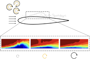
In the presence of FST forcing, the mean-flow topology of the LSB changes. In particular, a slight delay of boundary-layer separation is observed and the height of the LSB decreases significantly with the mean transition position advancing upstream, as can be observed in the contours of mean streamwise velocity and  $u_{rms}$ presented in figure 7. For the sake of brevity only three configurations are presented, C1 ( $Tu=1.21\,\%$), C5 ( $Tu=2.97\,\%)$ and C7 ( $Tu=6.26\,\%$) where no LSB is observed. The measurements, in accordance with previous studies (Simoni et al. Reference Simoni, Lengani, Ubaldi, Zunino and Dellacasagrande2017; Istvan & Yarusevych Reference Istvan and Yarusevych2018; Hosseinverdi & Fasel Reference Hosseinverdi and Fasel2019), show that, with the increase of $Tu$, the streamwise extent of the separation bubble is reduced, as a result of an earlier onset of pressure recovery, caused by the shear layer transitioning in the aft position of the LSB. The length of the bubble decreases due to higher initial forcing or higher amplification rate. This has an impact on the reattachment point, leading to a shorter bubble. The displacement effect of the boundary layer will be reduced and will modify the pressure gradient and the re-adjustment results in the small change in the location of the separation. This has been reported quite widely in the literature, where Marxen & Henningson (Reference Marxen and Henningson2011) have shown quantitative validation by varying the magnitude of initial perturbation. Finally, the height of the LSB is also reduced, and has been also observed in previous experimental and numerical studies (Simoni et al. Reference Simoni, Lengani, Ubaldi, Zunino and Dellacasagrande2017; Istvan & Yarusevych Reference Istvan and Yarusevych2018; Hosseinverdi & Fasel Reference Hosseinverdi and Fasel2019).

Figure 7. Contours of the mean streamwise velocity ( $U$) and the r.m.s. of the fluctuating streamwise velocity ( $u_{rms}$) for exemplary configurations subjected to elevated levels of FST (a) 1.21 % (b) 2.97 % and (c) 6.28 %.
The delay in boundary-layer separation is thought to be due to the increased initial energy amplitude introduced into the boundary layer due to the FST, resulting in separation occurring further downstream, shortening the bubble due to the earlier transition. The resulting boundary-layer displacement effect modifies the upstream pressure field, leading to separation delay. The accurate quantification in the downstream shift of  $x_{S}$ with increased $Tu$ is not possible here since it is smaller than the uncertainty in its determination. However, as mentioned in the previous section, the location of the separation position would have little impact on the boundary-layer transition mechanisms, hence it is not of great interest in the present study. The reattachment point is somewhat easier to determine, as its variation with $Tu$ is larger than for the separation point since the inflectional nature of the profile is not clearly distinguishable. In the current configuration the reattachment point for the configurations where an LSB was observed are presented in table 3. Referring to the boundary-layer integral parameters presented in figure 8, the streamwise location of the peak in the displacement thickness ( $\delta _{1}$) is accompanied by an increase in momentum thickness ( $\delta _{2}$), and can be associated with the mean transition of the separated shear layer. Consequently, the shape factor ( $H=\delta _{1}/\delta _{2}$) also reaches a maximum value at this position, corresponding to the maximum height of the LSB. Increasing the level of $Tu$ results in a systematic decrease in $\delta _{1}$, corresponding to the decrease in the wall-normal height of the LSB. Additionally, a higher $Tu$ results in a less pronounced value of $\delta _{1}$ and an upstream shift in the location of the maxima. This, combined with an earlier onset of momentum thickness growth, indicates earlier transition. When the levels of $Tu$ pass a certain threshold, the existence of a LSB is in question as $H$ does not exhibit any streamwise growth. In the current experimental configuration the level of $Tu$ at which the bubble was suppressed is 4.26 % (C6). Configuration C5 ( $Tu=2.97\,\%$) could still have an LSB as an amplified frequency band is observed in the PSD and will be discussed in more detail in § 3.2. Furthermore, for all the configurations, $H$ departs from a value expected for a laminar boundary layer ( $H>2.5$) and asymptotically levels off to that expected for a turbulent boundary layer ( $H<2$), signifying us that transition occurs within the HWA measurement domain. The current results exhibit the same systematic trends in mean bubble topology and integral parameters as in the DNS of Hosseinverdi & Fasel (Reference Hosseinverdi and Fasel2019) and PIV measurements of Istvan & Yarusevych (Reference Istvan and Yarusevych2018).

Figure 8. Effect of FST on integral shear layer parameters: (a) displacement thickness ( $\delta _{1}$), (b) momentum thickness ( $\delta _{2}$) and (c) shape factor ( $H$). Turbulence intensity increases from dark red to dark blue, refer to table 2. Dashed lines denote uncertainty for the natural case.
Table 3. Effect of FST on mean transition ( $x_{T}/c \pm 0.025$) and reattachment ( $x_{R}/c\pm 0.025$). The reattachment position was not measured in the configuration with $Tu=0.64\,\%$.

Upon inspection of the  $u_{rms}$ profiles in the wall-normal direction from figure 9, increasing the $Tu$ results in an upward shift in the maxima when compared with the baseline case. This behaviour suggests a shift in the transition mechanism, where a non-modal instability would exhibit the maximum $u_{rms}$ values further away from the wall than a modal instability. Moreover, increasing the FST intensity yields magnitudes of $u_{rms}/U_{e}\approx 10\,\%$ which is common for streaks (Westin et al. Reference Westin, Boiko, Klingmann, Kozlov and Alfredsson1994; Fransson et al. Reference Fransson, Matsubara and Alfredsson2005), and is larger than what is observed for pure modal transition ( $u_{rms}/U_{e}\approx 1\,\%$, Arnal & Julien Reference Arnal and Julien1978). The co-existence of modal and non-modal instabilities in attached boundary layers has been found to have similar effects on the maximum of the $u_{rms}$ peak (Veerasamy, Atkin & Ponnusami Reference Veerasamy, Atkin and Ponnusami2021). Moreover, increasing $Tu$ decreases the rate at which the fluctuations diminish into the free stream. In the configurations where $Tu$ is large enough to suppress the bubble, the $u_{rms}$ peak gradually shifts downwards, suggesting the flow is undergoing a change in transition mechanism and will be discussed later.

Figure 9. Chordwise development of the r.m.s. of the fluctuating streamwise velocity component ( $u_{rms}$) for chordwise positions of (a) 0.250 $c$ (b) 0.350 $c$ (c) 0.425 $c$ (d) 0.500 $c$ and (e) 0.575 $c$ subjected to FST.
Using acoustic forcing, Kurelek et al. (Reference Kurelek, Kotsonis and Yarusevych2018) found that the initially increased amplitude in the boundary layer upstream of the flow resulted in the bubble being shorter and thinner, similar to what has been observed in Marxen & Henningson (Reference Marxen and Henningson2011) in DNS simulations. In the same manner, FST increases the initial forcing in the boundary layer, resulting in similar effects on the mean-flow topology as with different forcing techniques. The impact forcing has on the bubble is that it modifies the wall-normal height, which would have an effect on the modal instability mechanism in the separated boundary-layer profile. The eigenfunctions can recover features of both Tollmien–Schlichting and KH instabilities where the bubble's height can modify the two mechanisms’ relative importance (Rist & Maucher Reference Rist and Maucher2002).
3.2. Disturbance growth and instability
3.2.1. Spectral analysis
The PSD of the streamwise velocity fluctuations was calculated for each configuration, with the chordwise evolution presented in figure 10. In the cases where an LSB was present, the PSD exhibits a characteristic frequency band amplified downstream (cf. figure 10a–g). When the LSB was subjected to FST, the chordwise development and distribution of the spectra were significantly modified. First, the unstable frequency band is broadened, which is a consequence of significant energy content within a larger range of frequencies in the FST, resulting in measurable velocity fluctuations over a larger frequency range earlier upstream. Second, increasing the FST level results in the unstable frequency band being slightly shifted to a higher frequency range than the natural case. For example, increasing the FST level from the baseline to a value of  $Tu=1.23\,\%$ results in the frequency band being shifted from 110–150 to 160–200 Hz (cf. figure 10a,d). Referring to figure 10(a–g), the unstable frequency band is propagated upstream of the separation point due to the separation bubble's streamwise oscillation. The highest-frequency wave packet is found to occur in the highest $Tu$ case, which was 255–295 Hz, wherein the highest cases ( $Tu>4\,\%$, figure 10h,i) no clear frequency band is observed and is thought to be due to the LSB not being present anymore, implying a change in the instability mechanism. The frequency shift of the wave packet is attributed to the decreased size of the LSB and has been observed in Hosseinverdi & Fasel (Reference Hosseinverdi and Fasel2019). Current results suggest that, in the configurations that are subjected to a turbulence intensity of $Tu<3\,\%$, the harmonic of the frequency band is still observed (cf. figure 10b,f,e), which could suggest that, in the presence of moderate levels of FST, the secondary instability of the primary modal instability could still be present. The secondary instability is a harmonic of the primary modal instability and takes effect in the aft portion of the bubble where vortex shedding occurs. In past studies, it has been reported to be an elliptic instability (Marxen, Lang & Rist Reference Marxen, Lang and Rist2013), amplifying disturbances with spanwise wavelengths of the order of the size of the shed vortices, resulting in spanwise distortion and waviness in the vortex filament and the presence of streaks could have an effect on this mechanism. The current results indicate that if $Tu$ is increased to a certain level, the harmonic of the wave packet is barely noticeable (cf. figure 10g), suggesting that there is a certain threshold of FST forcing which will ‘bypass’ the secondary instability, which will still exist in moderate cases and is in agreement with the numerical simulations of Li & Yang (Reference Li and Yang2019). Finally, the impact of the integral length scale has a negligible effect on the unstable frequency range of the wave packet.

Figure 10. Chordwise evolution of the PSD of the streamwise velocity fluctuations at the maximum location of  $u_{max}$ inside the boundary layer for each configuration. The frequency bands correspond to the vertical dashed lines which indicate the most amplified frequency band used in the stability analysis in the following section. Red and blue curves denote $x_{S}$ and $x_{R}$, respectively. NB: spectra are separated by an order of magnitude for clarity.
Pauley, Moin & Reynolds (Reference Pauley, Moin and Reynolds1990) proposed a scaling of the most unstable frequency in an LSB, in the form of a Strouhal number defined as
 \begin{equation} St_{\delta_{2},sep}= \frac{F\delta_{2,s}}{U_{e,s}}, \end{equation}
where  $F$ is the most amplified frequency observed in the experiment, $\delta _{2,s}$ and $U_{e,s}$ are the momentum thickness and boundary-layer edge velocity at separation, respectively. Inspired by the analysis of Rodríguez & Gennaro (Reference Rodríguez and Gennaro2019) and Rodríguez et al. (Reference Rodríguez, Gennaro and Souza2021), who compared the value of $St_{\delta _{2,sep}}$ for past experiments on LSBs, figure 11 compares the value of $St_{\delta _{2,sep}}$ as a function of $Tu$ (for the cases where an LSB was observed). In the present work, $St_{\delta _{2,sep}} = 0.0062$ for the unforced bubble which is close to the value of $St_{\delta _{2,sep}} = 0.0069$ proposed by Pauley et al. (Reference Pauley, Moin and Reynolds1990) for 2-D numerical simulations of an LSB. However, increasing $Tu$ causes $St_{\delta _{2,sep}}$ to increase compared with the baseline case, approaching values closer to what was proposed by Rodríguez et al. (Reference Rodríguez, Gennaro and Souza2021) of $St_{\delta _{2,sep}}=0.01 \unicode{x2013} 0.012$ for a bubble acting as a global oscillator. Data from Istvan & Yarusevych (Reference Istvan and Yarusevych2018) also suggest this effect and Pauley (Reference Pauley1994) found that $St_{\delta _{2,sep}}=0.0124 \unicode{x2013} 0.0136$ in 3-D unforced numerical simulations twice as large of what was observed for 2-D simulations. Therefore, the increased values of $St_{\delta _{2,sep}}$ suggests that the presence of FST (or increased levels of forcing) could favour the inherent 3-D nature of the transition process in the LSB. Furthermore, Rodríguez & Gennaro (Reference Rodríguez and Gennaro2019) found that increasing the recirculating velocity in the bubble increased the values of $St_{\delta _{2,sep}}$ which could manifest here as well, since the LSBs subjected to FST are smaller in size for the same convective velocity, which would result in larger levels of re-circulation inside the bubble. Finally, discrepancies in the values of $St_{\delta _{2,sep}}$ can be associated with the set-up and configurations of experiments. For instance, flat plates (with imposed pressure gradients) vs aerofoils, the surface finish of the models, and the inherent bias of the different experimental techniques. Moreover, the different Reynolds numbers and pressure gradients would modify the mean bubble's height and length, which could also result in the differences in the value of $St_{\delta _{2,sep}}$. In particular, under certain conditions (Gaster Reference Gaster1967), the formation of a ‘long’ bubble can occur. However, it is outside of the scope of the current study, which focuses on a ‘short’ bubble.

Figure 11. The dimensionless frequency,  $St_{\delta _{2,sep}}$, plotted against the turbulence intensity, $Tu$, for the present results and experimental data from the literature.
The intermittent global motion of the separated shear layer in an LSB is often referred to as flapping and is known to occur at significantly lower frequencies than 2-D vortex roll-up and shedding (Zaman, McKinzie & Rumsey Reference Zaman, McKinzie and Rumsey1989; Michelis, Yarusevych & Kotsonis Reference Michelis, Yarusevych and Kotsonis2017), depending on the incoming perturbations, which can change the bubble's stability characteristics. Following the conventions from Michelis et al. (Reference Michelis, Yarusevych and Kotsonis2017), the frequency normalised by the Strouhal number based on the displacement thickness
 \begin{equation} St_{\delta_{1},sep}= \frac{F\delta_{1,s}}{U_{e,s}}. \end{equation}
We note that this Strouhal number should not be confused with the Strouhal number proposed by Pauley et al. (Reference Pauley, Moin and Reynolds1990). Moreover, for assessing flapping experimentally, a temporal signal is extracted at a streamwise location corresponding to the approximate position of the mean separation point,  $x_{s}$, and at a wall-normal location of $y = \delta _{1}$. At this same position in the LSB, Michelis et al. (Reference Michelis, Yarusevych and Kotsonis2017) demonstrated that the flapping of an unforced LSB manifested itself at low frequencies below $St_{\delta _{1,sep}}= 0.005$. The results shown in figure 12 suggest that flapping is also manifesting as we observe an increase in spectral content when $St_{\delta _{1,sep}} < 0.005$. When the $Tu$ level is above the baseline, the increase of spectral content is less evident, suggesting that the level of free-stream disturbance could affect bubble flapping.

Figure 12. The PSD of the streamwise velocity fluctuations for the unforced LSB (black), the LSB subjected to  $Tu = 0.64\,\%$ (red) and $Tu = 1.21\,\%$ (blue) at a height of $y = \delta _{1}$ at the separation point. The Strouhal number is scaled by $\delta _{1}$, and should not be confused with the Strouhal number scaled with $\delta _{2}$ in figure 11.
3.2.2. Disturbance energy growth
The effect of increasing the level of  $Tu$ on the chordwise evolution of the disturbance energy growth $(E = u_{rms}^{2}/U^{2}_e)$ is presented in figure 13(a), where the trend of disturbance growth gradually changes from exponential, at lower levels of $Tu$, to algebraic for the more extreme $Tu$ levels, where energy saturation is observed earlier. These different energy growth behaviours suggest that different instability mechanisms were present in the flow, and their contribution to the transition process depends on the level of the free-stream forcing. Figure 13(b) shows the energy growth of the filtered disturbances for the most amplified frequency band (corresponding to the modal instability in the LSB) obtained from the PSD (cf. figure 10). In the natural case, low levels of disturbance growth are present before the separation point, and further downstream, exponential amplification of the disturbances is observed. In the cases where the flow is subjected to additional FST, the initial energy amplitude is significantly higher than in the natural case. The initial energy in the boundary layer increases with $Tu$, with higher energy levels suggesting the presence of streaks, as commonly observed in experiments on transition induced by FST in boundary layers subjected to no adverse pressure gradient.

Figure 13. Energy growth of disturbances for (a) integrated over the entire energy spectrum and (b) integrated over the frequency range of the most amplified wave packet plotted on a semi-log scale to show modal growth. Configurations where no LSB was detected, i.e. where no amplified frequency band was observed in the PSD, are not included for the filtered disturbance growth (cf. figure 10h,i). Maximum values of  $u_{rms}$ in the boundary layer are presented.
Referring to figure 13(b), the gradual reduction in the slope of the chordwise energy growth with increasing  $Tu$ would suggest that the non-modal instabilities become more dominant, which can be thought of as being in competition with the modal instabilities which grow exponentially. Once the turbulence forcing reaches a critical level, the exciting streaks in the boundary layer are too energetic to allow the flow to separate, resulting in the elimination of the modal via the non-modal instability (in the present work, approximately when $Tu>4\,\%$, since no inflection point is observed in the mean flow and no amplified frequency band in the PSD). Damping of the modal disturbance growth is attributed to the mean-flow deformation due to the influence of FST. In other words, external FST forcing reduces the size of the separation bubble, such that the region of instability growth is brought closer to the wall, resulting in damping effects of the disturbances in the shear layer. Previous experiments on forced bubbles found a damping effect on the disturbance growth. For example, Kurelek et al. (Reference Kurelek, Kotsonis and Yarusevych2018) found that both tonal and broadband acoustic forcing resulted in the damping of modal disturbances along with Yarusevych & Kotsonis (Reference Yarusevych and Kotsonis2017) and Marxen & Henningson (Reference Marxen and Henningson2011) who used a variety of forcing techniques and observed similar behaviour. Furthermore, the DNS investigation by Hosseinverdi & Fasel (Reference Hosseinverdi and Fasel2019) found similar trends in the energy growth with increased levels of $Tu$, albeit they did not show the behaviour when the bubble was suppressed, which in the present results is characterised by a high level of initial energy and evident algebraic growth of disturbances upstream of any possible separation location ( $Tu=6.26\,\%$, figure 13a).
The damping of the modal disturbances in the bubble could be due to the presence of streaks (Klebanoff modes) caused by the elevated levels of FST, which would introduce non-modal disturbances into the boundary layer. In the current set-up, streaks should appear for configurations where  $Tu>1\,\%$, which is a common threshold for zero-pressure-gradient boundary layers (Matsubara & Alfredsson Reference Matsubara and Alfredsson2001; Fransson et al. Reference Fransson, Matsubara and Alfredsson2005). The behaviour of the disturbance growth suggests the co-existence of modal and non-modal instability in the LSB when subjected to a critical level of FST. The experimental findings here agree with previous numerical results in the literature (Balzer & Fasel Reference Balzer and Fasel2016; Hosseinverdi & Fasel Reference Hosseinverdi and Fasel2019; Li & Yang Reference Li and Yang2019).
The impact of the integral length scale for a relatively constant  $Tu$ level on the disturbance growth is presented in figure 14, suggesting that the effect of the integral length scale on the transition in an LSB is very modest. The difficulty in achieving constant levels of $Tu$ with a varying $\varLambda _{u}$ is an experimental challenge, as shown by Fransson & Shahinfar (Reference Fransson and Shahinfar2020). The present work investigates three cases with a minimal variation in $Tu$ and a larger variation in $\varLambda _{u}$. It is observed that an increase in $\varLambda _{u}$ at the leading edge of the aerofoil for an almost constant $Tu$ appears to delay the growth and eventual saturation and breakdown of the disturbances and is in agreement Breuer (Reference Breuer2018), who suggested that the smaller scales were closer to that of the shear layer resulting in the receptivity of the boundary layer increasing. The impact of $\varLambda _{u}$ has been shown to have contradicting results in attached boundary-layer transition problems, where a variation of the integral length scale both advances (Jonáš et al. Reference Jonáš, Mazur and Uruba2000; Brandt et al. Reference Brandt, Schlatter and Henningson2004; Ovchinnikov, Choudhari & Piomelli Reference Ovchinnikov, Choudhari and Piomelli2008) and delays (Hislop Reference Hislop1940; Fransson & Shahinfar Reference Fransson and Shahinfar2020) boundary-layer transition. This contradiction led Fransson & Shahinfar (Reference Fransson and Shahinfar2020) to hypothesise a twofold effect of the integral length scale on boundary-layer transition subjected to FST. They found that, for a constant $Tu$ level, an optimal scale ratio exists between $\varLambda _{u}$ at the leading edge and the boundary-layer thickness at the transition position, which has a value of approximately 15. Interestingly, in the attached portion of the boundary layer of the three configurations tested, the advancement of the nonlinear growth of disturbances and eventual breakdown occurs when approaching this optimal value.

Figure 14. The chordwise evolution of the disturbance energy growth for configurations with a relatively fixed  $Tu$ and varying $\varLambda _{u}$. Maximum values of $u_{rms}$ in the boundary layer are presented.
However, it should be noted that the above studies were conducted on attached boundary layers. Hence, it is unclear whether meaningful comparisons can be made. For LSBs, Hosseinverdi & Fasel (Reference Hosseinverdi and Fasel2019) briefly suggested that the integral length scales ranging from 0.9 $\delta _{1}$ to 3 $\delta _{1}$ had little effect on the energy growth relative to $Tu$, and this is also observed in the experimental results here. Furthermore, a smaller integral length scale resulted in a higher initial level of disturbance energy in the boundary layer and has also been observed by Hosseinverdi (Reference Hosseinverdi2014). However, in their work, the saturation of the energy growth was found to be independent of $\varLambda _{u}$. Based on the experimental observations here and past numerical simulations, an effect of the integral length scale could be present, and further investigation is warranted. However, it is likely that the effect will be small compared with $Tu$, in light of the results here and those from Hosseinverdi & Fasel (Reference Hosseinverdi and Fasel2019).
3.2.3. Co-existence of a modal and a non-modal instabilities
The assertions made in the previous sections on the co-existence of modal and non-modal growths of disturbances in the LSB will be examined here through a linear stability analysis. Linear stability theory models the amplification of small-amplitude disturbances (Schmid & Henningson Reference Schmid and Henningson2000) and has been employed to study the convective streamwise amplification of disturbances in the LSB. The Orr–Sommerfeld equation is given by (3.3) and can reliably predict the primary amplification of instability waves for parallel flows and in the fore position of an LSB (Kurelek et al. Reference Kurelek, Kotsonis and Yarusevych2018)
 \begin{equation} \left(U - \frac{\varOmega}{\alpha}\right)\left(\frac{{\rm d}^2\tilde{v}}{{{\rm d} y}^2} - \alpha^2\tilde{v}\right) - \frac{{\rm d}^2U}{{{\rm d} y}^2}\tilde{v} ={-} \frac{{i}U_e\delta_1}{\alpha Re_{\delta_1}}\left(\frac{{\rm d}^4\tilde{v}}{{{\rm d} y}^4}- 2\alpha^2\frac{{\rm d}^2\tilde{v}}{{{\rm d} y}^2} + \alpha^4\tilde{v} \right) ,\end{equation}
where  $Re_{\delta _1}$ is the Reynolds number based on displacement thickness, $\tilde {v}$ is the wall-normal perturbation, $\varOmega$ is the angular frequency and the complex wavenumber is defined as $\alpha =\alpha _r+{i}\alpha _i$, where $i$ is the imaginary unit. When $\alpha _i>0$, the disturbance is attenuated and amplified when $\alpha _i<0$.
Calculations were conducted using ONERA's in-house stability code, where a spatial formulation of the problem is employed (Schmid & Henningson Reference Schmid and Henningson2000), such that  $\varOmega$ is defined and the eigenvalue problem is solved for $\alpha$, therefore modelling the convective amplification of single frequency disturbances. Equation (3.3) is solved numerically using Chebyshev polynomial base functions and the companion matrix technique to treat eigenvalue nonlinearity (Bridges & Morris Reference Bridges and Morris1984).
The mean streamwise velocity profiles at discrete streamwise locations are used as input for the LST calculations, making the analysis local, with the same methodology employed by Yarusevych & Kotsonis (Reference Yarusevych and Kotsonis2017) and Kurelek et al. (Reference Kurelek, Kotsonis and Yarusevych2018). Stability calculations are highly sensitive to noise due to the spatial resolution in experiments. Therefore, the LST analysis is conducted using hyperbolic tangent fits to experimental data, which have shown to provide reasonable stability predictions, being relatively insensitive to scatter in experimental data. The following modified hyperbolic tangent fit was used:
 \begin{equation} \frac{U}{U_{e}} = \frac{\tanh[a_{1}(y-a_{2})]+\tanh[a_{1}a_{2}]}{1+\tanh[a_{1} a_{2} ]}+a_{3}\frac{y}{a_{2}}\exp\left[{-}1.5\frac{y}{a_{2}}^{2}+0.5\right], \end{equation}
which was proposed by Dovgal, Kozlov & Michalke (Reference Dovgal, Kozlov and Michalke1994) and has been shown to suitably model separated boundary-layer profiles in several analytical applications (Boutilier Reference Boutilier2011; Boutilier & Yarusevych Reference Boutilier and Yarusevych2013) along with accurate linear stability predictions on HWA velocity profiles of separated shear layers (Boutilier & Yarusevych Reference Boutilier and Yarusevych2012). The profile edge velocity,  $U_{e}$, is estimated from the HWA measurements, while the coefficients $a_{1}-a_{4}$ are estimated through a least-squares curve fitting operation to the measured data. Exemplary velocity profiles and their corresponding fits for the configuration with $Tu=1.21\,\%$ are presented in figure 15. Furthermore, due to the difficulty in conducting stability calculations on experimental velocity profiles at low $Tu$ and Reynolds numbers, LST calculations for the baseline case are validated by conducting the analysis on both experimental (hyperbolic fit) and numerical (obtained from the boundary-layer solver, 3C3D) velocity profiles which were within acceptable agreement.

Figure 15. Measured mean velocity profiles (markers) in a forced condition ( $Tu=1.21\,\%$) and corresponding hyperbolic tangent fits (solid lines) used in LST computations.
A measure of the amplitude growth is quantified from LST through the computation of amplification factors and will be referred to as the  $N$-factor hereinafter. The $N$-factor as a function of streamwise position ( $x$) and frequency ( $F$) from LST calculations and is quantified by integrating $\alpha _{i}$ for the most amplified frequency in the positive $x$-direction
 \begin{equation} N(x,F) =\int_{x_{cr}}^{x}- \alpha_{i} \,{{\rm d}\kern0.06em x} , \end{equation}
where  $x_{cr}$ is the critical abscissa and corresponds to the location at which a perturbation at a non-dimensional frequency of $\varOmega$ is first amplified. The location of $x_{cr}$ is upstream of the hot-wire measurement region and, therefore, cannot be determined directly. However, as demonstrated by Jones, Sandberg & Sandham (Reference Jones, Sandberg and Sandham2010), Kurelek et al. (Reference Kurelek, Kotsonis and Yarusevych2018), Yarusevych & Kotsonis (Reference Yarusevych and Kotsonis2017) and Kurelek (Reference Kurelek2021), in the fore portion of the LSB the streamwise evolution of $\alpha _{i}$ can be approximated by a second-order polynomial. For example, Kurelek (Reference Kurelek2021) (HWA, Ch. 6) and Kurelek et al. (Reference Kurelek, Kotsonis and Yarusevych2018) (PIV) demonstrated that the ( $-\alpha _{i}$) obtained from LST calculations for four velocity profiles before and after the separation position could be used in the interpolation. Considering this, $x_{cr}$ can be determined by extrapolating the fit to $\alpha _{i}=0$. Experimentally, the $N$-factor is calculated as $N(x)=\ln (A(x)/A_{cr})$, where $A(x)$ denotes the maximum disturbance amplitude in the boundary layer for a given frequency band (band-pass filtered $u_{rms}$) and $A_{cr}$ denotes the initial disturbance amplitude that becomes unstable. A direct comparison of $N$-factor obtained from LST and experiment is not possible since, experimentally, the initial disturbance amplitude is not known and likely to be too small to be measured, only being detected well downstream of $x_{cr}$. Nevertheless, following Schmid & Henningson (Reference Schmid and Henningson2000), $N$-factors are matched at a reference location where the disturbance amplitude reaches 0.005 $U_{\infty }$, consequently allowing for an estimate of $A_{cr}$ for a given frequency band.
In the baseline configuration, the overlaid plot between PSD and the  $N$-factor shows that LST is capable of predicting the most amplified frequencies from experiment, with acceptable accuracy (10 % difference). For example, Kurelek et al. (Reference Kurelek, Kotsonis and Yarusevych2018) and Yarusevych & Kotsonis (Reference Yarusevych and Kotsonis2017) found a difference of 17 %, while stating this to be an acceptable range. A comparison with experimental $N$-factors further supports the validity of the LST predictions (cf. figures 16a and 17a), which reveals that the linear growth of disturbances is captured in the range $0.475 < x/c < 0.525$, comparable to the same analysis by Kurelek et al. (Reference Kurelek, Kotsonis and Yarusevych2018) who found LST to accurately capture the growth of disturbances in the range $0.42 < x/c < 0.46$ in their experiment. Furthermore, as the downstream saturation of the experimental $N$-factors begins to deteriorate, the agreement between LST due to nonlinear effects becomes significant. The eigenfunction of the most amplified frequency predicted by LST is presented in figure 18(a), and shows acceptable agreement with the experiment for the filtered fluctuating streamwise velocity profile in the wall-normal direction for the most amplified frequency band. The eigenfunction exhibits two distinct peaks at approximately $y/\delta _{1}=1$, corresponding roughly to the inflection point and $y/\delta _{1}=0.3$, which is indicative of a viscous modal instability (Veerasamy et al. Reference Veerasamy, Atkin and Ponnusami2021). Rist & Maucher (Reference Rist and Maucher2002) showed that Tollmien–Schlichting waves were more likely to emerge in LSBs with small wall-normal distances, and a KH instability in LSBs with higher wall-normal distances. Therefore, based on the agreement seen in the unstable frequencies, eigenfunctions and amplification rates (figures 16a, 18 and 17a), it is established that the employed LST analysis is justified for determining stability characteristics in the fore portion of the LSB.

Figure 16. Comparison between the  $N$-factors predicted by LST and the experimental spectra for (a) natural case ( $x=0.400c$); (b) $Tu=0.64\,\% \varLambda _{u} = 4.6\ {\rm mm}$ ( $x=0.425c$); (c) $Tu=1.21\,\% \varLambda _{u} = 8.7\ {\rm mm}$ ( $x=0.425c$); (d) $Tu=1.23\,\%, \varLambda _{u} = 10.3\ {\rm mm}$ ( $x=0.425c$); (f) $Tu=1.63\,\%, \varLambda _{u} = 12.3\ {\rm mm}$ ( $x=0.425c$); (g) $Tu=2.97\,\%, \varLambda _{u} = 15.4\ {\rm mm}$ ( $x=0.400c$). There are two different $y$-axes for the $N$-factor and the power from the PSD, therefore direct comparisons between the two are not to be made.

Figure 17. Comparison of experimental (markers) and LST (dashed line) predicted  $N$-factors for frequencies within the excitation bands from figure 10 for configurations where a LSB is present: (a) natural case; (b) $Tu=0.64\,\% \varLambda _{u} = 4.6\ {\rm mm}$; (c) $Tu=1.21\,\%, \varLambda _{u} = 8.7\ {\rm mm}$; (d) $Tu=1.23\,\%, \varLambda _{u} = 10.3\ {\rm mm}$; (e) $Tu=1.31\,\%, \varLambda _{u} = 8.3\ {\rm mm}$; (f) $Tu=1.63\,\%, \varLambda _{u} = 12.3\ {\rm mm}$; (g) $Tu=2.97\,\%, \varLambda _{u} = 15.4\ {\rm mm}$; initial disturbance amplitudes are estimated through matching LST and experimental $N$-factors.

Figure 18. Experimental filtered disturbance profiles in the wall-normal direction compared with the eigenfunction for the most amplified frequency from LST. Experimental streamwise disturbance profiles are computed by applying a bandpass filter corresponding to the lost amplified frequency band from the PSD. (a) Natural case; [110–150 Hz] at  $x=0.425c$, (b) $Tu=0.64\,\%, \varLambda _{u} = 4.6\ {\rm mm}$ [160–200 Hz] at $x=0.400c$, (c) $Tu=1.21\,\%, \varLambda _{u} = 8.7\ {\rm mm}$ [180–220 Hz] at $x=0.425c$, (d) $Tu=1.23\,\%, \varLambda _{u} = 10.3\ {\rm mm}$ [180–220 Hz] at $x=0.400c$, (e) $Tu=1.31\,\%, \varLambda _{u} = 8.3\ {\rm mm}$ [180–220 Hz] at $x=0.400c$, (f) $Tu=1.63\,\%, \varLambda _{u} = 12.3\ {\rm mm}$ [180–220 Hz] at $x=0.450c$ and (g) $Tu=2.97\,\%, \varLambda _{u} = 15.4\ {\rm mm}$ [255–295 Hz] at $x=0.425c$.
For the configurations where the LSB is subjected to elevated levels of FST, LST can predict the most amplified frequencies, spatial amplification and eigenfunctions, suggesting that a modal instability is still present at elevated levels of FST when the bubble is present. Counter-intuitively, FST forcing results in better agreement between LST and experiment and has been found in past experiments with increased forcing by Yarusevych & Kotsonis (Reference Yarusevych and Kotsonis2017), Kurelek et al. (Reference Kurelek, Kotsonis and Yarusevych2018) and Kurelek (Reference Kurelek2021) (Ch. 6), who found that LST was capable of predicting the convective growth of disturbances in LSBs subjected to plasma, tonal and broadband acoustic forcing. However, as Kurelek et al. (Reference Kurelek, Kotsonis and Yarusevych2018) noted, the critical caveat to be considered is that the degree to which LST and experiment agree is entirely dictated by the relevance of nonlinear effects for the particular disturbance mode being considered. Fully developed FST could act as a type of ‘broadband’ forcing, such that all unstable disturbance amplitudes are small, resulting in nonlinear effects and an improved agreement between LST and experiment. Therefore, current results support the assertions made by Kurelek et al. (Reference Kurelek, Kotsonis and Yarusevych2018), who found excellent agreement between LST and experiment for an LSB subjected to broadband acoustic forcing. The higher signal-to-noise ratio can also explain the improvement in the presence of forcing with FST.
Another explanation for the divergence between LST and experiment for configurations subjected to low levels of  $Tu$ could result from the bubble's wall-normal extent being larger compared with higher levels of $Tu$. The more considerable distance of the shear layer from the wall would foster other instabilities, such as a global oscillator (Rist & Maucher Reference Rist and Maucher2002) or even the global oscillator being preceded by the 3-D global instability as in Rodríguez et al. (Reference Rodríguez, Gennaro and Souza2021). Another possibility could be that a shear on structures in the direction opposed to the mean flow may lead to a non-modal instability through an Orr mechanism (Cherubini, Robinet & De Palma Reference Cherubini, Robinet and De Palma2010). Therefore, the augmented agreement between LST $N$-factor envelopes and experiments in configurations subjected to moderate levels of $Tu$ ( $1.3\,\%< Tu<2.97\,\%$) can be explained by these FST levels being effective in exciting Tollmien–Schlichting waves in the pre-separated shear layer. At these moderate $Tu$ levels, the nonlinear distortion of the mean flow due to the streaks does not impact their amplification, resulting in the Orr–Sommerfeld equation predicting the $N$-factor envelopes from experiment. At a high enough $Tu$ threshold, the mean-flow modification due to the presence of streaks is too significant, resulting in the growth of wave-like disturbances being inhibited and the divergence from LST and experiment.
Consequently, using the analysis employed by Yarusevych & Kotsonis (Reference Yarusevych and Kotsonis2017), Kurelek et al. (Reference Kurelek, Kotsonis and Yarusevych2018) and Kurelek (Reference Kurelek2021), the current results show that LST is capable of modelling the convective growth of disturbances in a bubble subjected to moderate FST levels. The critical difference is that forcing with elevated levels of FST ( $Tu>1\,\%$) can cause the generation of streaks, considered to be a convective non-modal amplification of disturbances (Matsubara & Alfredsson Reference Matsubara and Alfredsson2001; Fransson et al. Reference Fransson, Matsubara and Alfredsson2005; Fransson & Shahinfar Reference Fransson and Shahinfar2020). The disturbance profiles just before and after separation presented in figure 19 (non-modal) strongly suggest the existence of the non-modal growth or streaks (Klebanoff modes) as the profiles exhibit self-similar behaviour with the optimal disturbance profiles from the theoretical work of Andersson et al. (Reference Andersson, Berggren and Henningson1999) and Luchini (Reference Luchini2000), with the maximum value of $u_{rms}$ occurring near $y/\delta _{1}=1.3$ for all configurations with $Tu>1\,\%$. The current results demonstrate the self-similarity of the disturbance profiles over most of the boundary layer (cf. figure 19f–j). Outside the boundary layer, results do not tend to zero since FST is present, in contrast to theory, which has no free-stream disturbances outside the boundary layer. Furthermore, inside the LSB, the disturbance profiles also appear to agree well with theory. The slight downwards shift of the profile at the most advanced chordwise positions is due to the flow finishing the transition process. These observations made in figures 18 and 19(f–j, non-modal) implies the co-existence of both modal and non-modal instability mechanisms, confirming the observations in DNS (Hosseinverdi & Fasel Reference Hosseinverdi and Fasel2019) and experimental investigations (Istvan & Yarusevych Reference Istvan and Yarusevych2018; Verdoya et al. Reference Verdoya, Dellacasagrande, Lengani, Simoni and Ubaldi2021) on LSBs subjected to FST, along with the experimental results of Veerasamy et al. (Reference Veerasamy, Atkin and Ponnusami2021) for an attached boundary layer developing over a flat plate. In contrast, in configurations where $Tu<1\,\%$ (refer to figure 19(a–e), modal), wall-normal disturbance profiles do not agree with theoretical predictions and do not exhibit the same behaviour as for configurations with $Tu>1\,\%$, with the maxima of the peaks being in the range $y/\delta _{1}=0.3\unicode{x2013}0.5$, implying that there is no formation of streaks and that only a modal transition mechanism is present. The observation of damping behaviour on the disturbance growth presented in the previous section (figure 13) being due to the non-modal amplification of streaks is supported by the results in figure 19. The damping of disturbance growth in the bubble is also reflected in the LST predictions, as values of amplification are slightly lower for configurations subjected to elevated levels of FST, in line with what has been observed for laminar separation bubbles subjected to other methods of forcing (Marxen & Henningson Reference Marxen and Henningson2011; Marxen et al. Reference Marxen, Kotapati, Mittal and Zaki2015; Yarusevych & Kotsonis Reference Yarusevych and Kotsonis2017; Kurelek et al. Reference Kurelek, Kotsonis and Yarusevych2018). The damping of the convective disturbance growth is due to the streaks modifying the mean flow. Therefore, the wall-normal distance and the length of the LSB is reduced. This results in lower values of $\delta _{1}$ resulting in lower levels of modal amplification due to the increased viscosity effects.

Figure 19. Streamwise velocity disturbance profiles for configurations where LSB is subjected to turbulence of  $Tu<1\,\%$ (a–e) and $Tu>1\,\%$ (g–k) for chordwise positions of (a,f) 0.325 $c$ (b,g) 0.350 $c$ (c,h) 0.375 $c$ (d,i) 0.400 $c$ and (e,j) 0.425 $c$. Configurations with $Tu<1\,\%$: NG and C0 and $Tu>1\,\%$: C1–C5. Refer to table 2 for symbols.
One may argue that a more rigorous characterisation could be made with fine spanwise hot-wire measurements, however, this was not possible due to the experimental set-up. Nevertheless, the claim of the presence of streaks is valid based on the disturbance profiles (cf. figure 19), decreased energy growth rates (cf. figure 13) and observations from previous work.
Finally, when the bubble is subjected to a sufficient level of FST forcing ( $Tu > 3\,\%$, in the present configuration), the formation of an LSB is not observed in the experimental data, suggesting that there is a critical initial forcing amplitude which will generate streaks containing enough energy to suppress boundary-layer separation by promoting earlier transition. Figure 20 confirms the existence of non-modal instabilities growing in the streamwise direction for the values of $Tu$ where no separation was observed. Streamwise velocity disturbance profiles are in very good agreement with Andersson et al. (Reference Andersson, Berggren and Henningson1999) and Luchini (Reference Luchini2000), exhibiting a clear peak at $y/\delta _{1} \approx 1.3$, with profiles further downstream manifesting a lower wall-normal position of the maxima due to the flow undergoing transition and tending to a turbulent state where the peak in the fluctuating velocity component is closer to the wall. Furthermore, the $u_{rms}$ profiles exhibit no peaks below $y/\delta _{1} \approx 1.3$, in stark contrast to what is observed in configurations containing a LSB. At the highest levels of FST, the bubble could be suppressed due to the boundary layer transitioning before the strong adverse pressure-gradient region, which promotes separation. However, the results could also suggest the suppression of laminar separation due to streaks (at least for the current experimental configuration), which is supported by the recent numerical investigation by Xu & Wu (Reference Xu and Wu2021). They found that free-stream vortical disturbances of moderate level prevent the separation in a boundary-layer flow over a plate or concave wall, suggesting that the strong mean-flow distortion associated with the nonlinear streaks or Görtler vortices prevents separation. The simulations by Xu & Wu (Reference Xu and Wu2021) found that streaks with maximum amplitudes of approximately 12 % suppressed separation, whereas, at lower amplitudes, separation would still occur. A similar phenomenon could exist in our results, where critically energetic streaks generated by sufficiently elevated FST can suppress separation. In these cases, as in Xu & Wu (Reference Xu and Wu2021), we also observe streak amplitudes in the range of 10 %–15 % of the free-stream velocity, although, at lower amplitudes, an LSB is still present.

Figure 20. Chordwise evolution of the disturbance profiles scaled with  $u_{rms,max}$ for chordwise positions of (a) 0.250 $c$, (b) 0.300 $c$, (c) 0.325 $c$, (d) 0.350 $c$, (e) 0.375 $c$, (f) 0.400 $c$, (g) 0.425 $c$, (h) 0.450 $c$, (i) 0.475 $c$, (j) 0.500 $c$. Black line denoted theoretical optimal perturbation profile by Luchini (Reference Luchini2000). Configurations C6 and C7: refer to table 2 for symbols.
4. Concluding remarks
The present investigation examines the effects of varying the free-stream turbulence intensity and integral length scale on the flow development and transition in a LSB. The LSB develops over the suction side of a NACA0015 aerofoil at a chord-based Reynolds number of 125 000 and angle of incidence of  $2.3^\circ$ in a low FST open circuit wind tunnel. Free-stream turbulence was generated in a controlled manner using regular and fractal grids resulting in a wide range of levels of turbulence intensity and integral length scales. The streamwise evolution of FST and the flow field were characterised using HWA. Eight free-stream flow configurations were tested, three with a fixed turbulence intensity level but a variable integral length scale.
The results exhibit that elevated levels of FST reduce the size of the mean bubble flow topology, advancing the transition position and decreasing the size of the bubble, with its eventual elimination at the highest levels. In the LSB, the convective development of an unstable frequency band is observed and is broadened with the addition of FST, a consequence of more significant energy content within a broader range of frequencies from the FST. The presence of FST also shifts the most amplified frequency band to a higher spectral range due to smaller wall-normal and streamwise lengths of the bubble when excited. In the baseline case, when the most amplified frequencies are non-dimensionalised through the use of a Strouhal number based on the boundary-layer momentum thickness at separation,  $St_{\delta _{2,sep}}$, an agreement is found with Pauley et al. (Reference Pauley, Moin and Reynolds1990). However, increasing $Tu$ causes $St_{\delta _{2,sep}}$ to increase when compared with the baseline case, approaching values closer to what was observed by Rodríguez et al. (Reference Rodríguez, Gennaro and Souza2021).
The presence of streaks is observed for configurations with  $Tu>1\,\%$, with unfiltered profiles agreeing remarkably well with the theoretical optimal perturbation profile at multiple chordwise positions before and inside the LSB. The mechanism of disturbance energy growth gradually changes from an exponential one, at lower levels of $Tu$, to an algebraic one for the more extreme $Tu$ levels, growing until the energy saturates. In the configuration where a bubble is present, band-pass filtered (corresponding to the most amplified frequency range) values of disturbance energy reveal the gradual reduction in the slope of the chordwise energy growth with increasing $Tu$, suggesting that the non-modal instabilities become more dominant, which can be thought of as competing with the modal instabilities. Once the turbulence forcing reaches a critical level, $Tu\approx 4\,\%$ in the present study, the streaks in the boundary layer are too energetic to allow the flow to separate, ensuing in the elimination of the modal instability via the non-modal instability and suppressing the formation of the bubble. The damping of the streamwise growth of disturbances is due to the presence of streaks (Klebanoff modes) caused by the elevated levels of FST, which change the mean-flow topology of the bubble through the introduction of non-modal disturbances into the boundary layer. Finally, for a relatively fixed level of $Tu$, the variation of $\varLambda _{u}$ has modest effects; however, a slight advancement of transition with the decrease in $\varLambda _{u}$ is observed.
Local linear stability analysis is shown to accurately model incipient distance growth for the unexcited turbulence case, in agreement with previous work (Yarusevych & Kotsonis Reference Yarusevych and Kotsonis2017; Kurelek et al. Reference Kurelek, Kotsonis and Yarusevych2018; Kurelek Reference Kurelek2021). Moreover, good agreement between LST eigenfunctions and filtered experimental  $u_{rms}$ profiles and the prediction of the most amplified frequencies is found. In the presence of elevated turbulence, LST predicts the growth of disturbances and unstable frequencies with acceptable accuracy. Counter-intuitively, an augmented agreement between experiment and LST for $N$-factor envelopes was present in configurations subjected to moderate levels of FST and was thought to be due to the turbulence being effective in exciting the viscous modal instabilities in the pre-separated shear layer. Additionally, filtered $u_{rms}$ profiles were representative of those predicted by LST and resembled those which are expected in the presence of modal visco-inflectional instabilities. Therefore, the current work provides rigorous experimental evidence on the co-existence of modal and non-modal instabilities in a laminar separation bubble.
Funding
Supported by internal funding of ONERA and ISAE–SUPAERO.
Declaration of interests
The authors report no conflict of interest.


