2.1. Mass conservation across the Knudsen layer

Assuming an infinitely thin Knudsen layer, mass conservation requires that

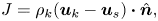(2.1)\begin{equation} J = \rho_k({\boldsymbol{u}_k} - {\boldsymbol{u}_s})\boldsymbol{\cdot} \hat{\boldsymbol{n}}, \end{equation}

where $\rho$ is the density, $\boldsymbol {u}$ is the velocity and $\hat {\boldsymbol {n}}$ is the normal outward unit vector. The immiscibility of $B$ in $A$ results in a vanishing mass flux of $B$ across the interface, such that the evaporation mass flux equals the mass diffusion flux of $A$, which can be written as

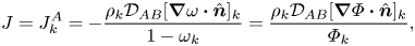(2.2)\begin{equation} J = J_k^A ={-}\frac{\rho_k\mathcal{D}_{AB} [\boldsymbol{\nabla}\omega \boldsymbol{\cdot} \hat{\boldsymbol{n}}]_k}{1-\omega_k}=\frac{\rho_k\mathcal{D}_{AB} [\boldsymbol{\nabla}\varPhi \boldsymbol{\cdot} \hat{\boldsymbol{n}}]_k}{\varPhi_k}, \end{equation}

where $\omega$ is the mass fraction of $A$, and $\varPhi = 1 - \omega$. Here, we consider the case where the total pressure in the gas domain remains unchanged (i.e. ${Ma} \ll 1$). In the case of high Mach number, the pressure relaxation process in the gas domain needs to be accounted for to find the change in pressure. To proceed, a kinetic model within the Knudsen layer (e.g. the analytical TED-SRT model or the semi-empirical HK model) needs to be used to predict $J$.

2.2. The HK-based mixed boundary condition

Assuming that the Knudsen layer is not too far from thermodynamic equilibrium and the velocity profile in the gas domain is Maxwellian, Struchtrup et al. (Reference Struchtrup, Beckmann, Rana and Frezzotti2017) proposed the following kinetic model in a pure vapour environment, based on the extension of the Onsager–Casimir reciprocity relations:

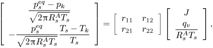(2.3)\begin{equation} \left[ \begin{array}{c} \dfrac{p_s^{eq}-p_k}{\sqrt{2 {\rm \pi}R_s^A T_s}} \\[10pt] -\dfrac{p_s^{eq}}{\sqrt{2 {\rm \pi}R_s^A T_s}} \dfrac{T_s-T_k}{T_s} \end{array} \right] = \left[ \begin{array}{cc} r_{11} & r_{12} \\ r_{21} & r_{22} \end{array}\right] \left[ \begin{array}{c} J \\[4pt] \dfrac{q_v}{R_s^A T_s} \end{array} \right], \end{equation}

where coefficients $r_{11}=1/{\rm \pi} +9/32$, $r_{12}=r_{21}=1/16+1/(5{\rm \pi} )$, $r_{22}=1/8+13/(25{\rm \pi} )$, $p_s^{eq}$ is the equilibrium vapour pressure of species $A$ and $q_v$ is the heat flux adds to the vapour. In the case of a negligible change of sensible heat inside the droplet, $q_v=-J \mathcal {L}$, where $\mathcal {L}$ is the latent heat of evaporation. The above expression is an extension of the HK model taking into account the Stefan flow due to net evaporation, with the additional assumption $\sigma _e=\sigma _c=1$. It also predicts the temperature jump across the Knudsen layer, which is commonly ignored in the literature. As shown by Persad & Ward (Reference Persad and Ward2016), assuming either $T_k = T_s$ or $\sigma _e = \sigma _c$ does not introduce major discrepancies compared with experimental results (${\leqslant }5\,\%$), but making both assumptions simultaneously forces the Knudsen layer into equilibrium, which could lead to significant errors. When applied in an inert gas environment, while the form of (2.3) might hold as long as the Knudsen layer is not too far from equilibrium, i.e. a linear irreversible process, the coefficients and $p_s^{eq}$ should be corrected by taking into account inert gases. The effect of inert gases on the temperature jump is evidenced by the empirical correlation (2.4) proposed by Holyst et al. (Reference Holyst, Litniewski, Jakubczyk, Zientara and Woźniak2013b). Equation (2.4) is based on curve fitting of data obtained from molecular dynamic (MD) simulations of the evaporation of a droplet made of a Lennard–Jones fluid in inert gases and reads as

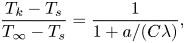(2.4)\begin{equation} \frac{T_k - T_s}{T_{\infty} - T_s}=\frac{1}{1+a/(C\lambda)}, \end{equation}

where $C$ is a fitting parameter calculated to be 2.35, and $\lambda$ is the mean free path of inert gas molecules. Equation (2.4) shows that a smaller $\lambda$ leads to a smaller temperature jump. This makes sense because the thermalisation process becomes more efficient as the collision frequency increases at reduced $\lambda$.

When the liquid surface is assumed to be at thermodynamic equilibrium, $p_s^{eq}$ can be determined by equating the chemical potential of the liquid phase $\mu ^l$ and that of the vapour phase $\mu ^v$. In order to find the change of chemical potential due to the presence of inert gases, we consider an isothermal gas addition process. The chemical potentials of the liquid phase and vapour phase of $A$ in the absence of any inert gas at temperature $T_s$ and pressure $p_s^\star$ are denoted by $\mu ^{l\star }$ and $\mu ^{v\star }$. As the inert gas is added to the system to reach a new equilibrium at increased total pressure $p_s$, one obtains

(2.5)\begin{equation} \mu^{l}(T_s, p_s) - \mu^{l\star} (T_s, p_s^\star) = \mu^{v}(T_s, p_s^{eq}) - \mu^{v\star}(T_s, p_s^\star). \end{equation}

Applying the Gibbs–Duhem equation yields

(2.6)\begin{equation} \int_{p_s^\star}^{p_s} v^l\,{\rm d}p = \int_{p_s^\star}^{p_s^{eq}} v^v\,{\rm d}p, \end{equation}

where $v^l$, $v^v$ and $v^{v\star }$ are molar volume of $A$ in liquid phase, and the vapour phase with and without inert gas, respectively. In the case of constant liquid molar volume and ideal gases, one obtains

(2.7)\begin{equation} p_s^{eq} = p_s^\star(T_s)\exp(\overline{v_s}),\quad \mbox{with}\ \overline{v_s} = v^l\left(\frac{1}{v^v}-\frac{1}{v^{v\star}}\right). \end{equation}

It appears from (2.7) that the exponential correction factor could become significant as the specific volume ratio increases, e.g. at high system pressure or low gas temperature. Note that the assumption of ideal gas needs to be corrected at high pressure or very low temperature. To assess the value of $p_s^\star$, the Clausius–Claperon equation – which is derived assuming (i) an ideal gas law, (ii) negligibly small gas phase density (compared with that of the liquid phase) and (iii) constant latent heat – can be integrated between the local equilibrium conditions at far field (i.e. outside the boundary layer) and that at the liquid surface. One obtains

(2.8)\begin{equation} p_s^\star = p_{\infty} \exp\left[\frac{\mathcal{L}}{R_s^A}\left(\frac{1}{T_\infty^{sat}}-\frac{1}{T_s}\right)\right], \end{equation}

where all properties at infinity are labelled with the subscript $\infty$. In the previous expression, $T_{\infty }^{sat}$ is the saturated temperature at $p_\infty$.

By combining (2.2), (2.3), (2.7) and (2.8), and accounting for the surface tension $\sigma _T$ based on Kelvin's law, we obtain the following mixed kinetic-diffusion boundary condition based on HK model:

(2.9)\begin{align} &\sqrt{\frac{1}{2{\rm \pi} R_s^A T_s}}\left\{c_1 p_{\infty} \exp\left[\frac{\mathcal{L}}{R_s^A}\left(\frac{1}{ T_{\infty}^{sat}}-\frac{1}{T_s}\right)+\overline{v_s}+\frac{\bar{\sigma}}{a}\right]-\left(c_1+c_2 \overline{\Delta T}\right)p_k^A \right\}\nonumber\\ &\quad = \frac{\rho_k\mathcal{D}_{AB} [\boldsymbol{\nabla}\varPhi \boldsymbol{\cdot} \hat{\boldsymbol{n}}]_k}{\varPhi_k}, \end{align}

where $c_1=r_{22}/(r_{11}r_{22}-r_{12}^2)$, $c_2=c_1 r_{11}/r_{22}$ and $\bar {\sigma } = 2\sigma _T/(R_s^A T^l \rho ^l)$.

2.3. The TED-SRT-based mixed boundary condition

Combining the analytical TED-SRT formulation derived by Persad & Ward (Reference Persad and Ward2016), i.e. (1.2a,b), together with (2.2), (2.7) and (2.8), and accounting for the surface tension, the following mixed boundary conditions can be derived:

(2.10)\begin{equation} \sqrt{\frac{1}{2{\rm \pi} R_s^A}}\left\{\hat{\sigma}_e\frac{\left\{p_{\infty} \exp\left[\dfrac{\mathcal{L}}{R_s^A}\left(\dfrac{1}{T_{\infty}^{sat}}-\dfrac{1}{T_s}\right)+ \overline{v_s}+\frac{\bar{\sigma}}{a}\right]\right\}^2}{p_k^A\sqrt{T_s}}-\sigma_c \frac{p_k^A}{\sqrt{T_k}}\right\} = \frac{\rho_k\mathcal{D}_{AB} [\boldsymbol{\nabla}\varPhi \boldsymbol{\cdot} \hat{\boldsymbol{n}}]_k}{\varPhi_k}. \end{equation}

2.4. Dimensionless forms of the mixed boundary conditions

To make the mixed kinetic-diffusion boundary conditions (2.9) and (2.10) dimensionless, the initial droplet radius $a_0$, the initial Stefan flow gas velocity $\mathcal {D}_{AB}/a_0$ and the quantity $a_0^2/\mathcal {D}_{AB}$ are chosen as the typical length, velocity and time, respectively. The quantity $\rho _\infty$ is chosen as the typical gas density, such that the typical evaporative mass flux becomes $\rho _\infty \mathcal {D}_{AB}/a_0$.

The mixed boundary condition based on the TED-SRT model (2.10) can be written in a dimensionless form as

(2.11)\begin{equation} \frac{\ln({{B}_M} + 1)}{{{Pe}_k}}=\frac{\bar{p}^2\exp(2\chi) \hat{\sigma}_e\sqrt{1+\overline{\delta T}}\left[\varepsilon(\varPsi+1-\varPhi_\infty)^{{-}1}-(\varepsilon-1)\right]^2-\sigma_c}{(1-\varPhi_\infty + \varepsilon\varPhi_\infty)^{{-}1}(1-\kappa)^{1/2}[\varepsilon(\varPsi+1-\varPhi_\infty)^{{-}1}-(\varepsilon-1)]}, \end{equation}

where

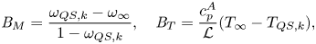(2.12a)$$\begin{gather} {{B}_M} = \frac{\omega_{QS,k}-\omega_\infty}{1-\omega_{QS,k}},\quad {{B}_T} = \frac{c_p^A}{\mathcal{L}}(T_\infty-T_{QS,k}), \end{gather}$$

(2.12b)$$\begin{gather}{{Pe}_k} = \frac{u_k a}{\mathcal{D}_{AB}},\quad u_k=\left(\frac{ R_s^A T_\infty}{2{\rm \pi}}\right)^{1/2},\quad \bar{p}=\frac{p^{{\star}}(T_\infty)}{p_\infty}, \quad \varepsilon=\frac{M^A}{M^B}, \end{gather}$$

(2.12c)$$\begin{gather}\varPsi=\frac{\varPhi_\infty {{B}_M}}{{{B}_M}+1},\quad \chi=\frac{\gamma}{\gamma-1} \left(\frac{1}{{{Ja}}}-\frac{1+\overline{\delta T}}{{{Ja}}-{{B}_T}}\right)+\overline{v_s}+\frac{\bar{\sigma}}{a}, \end{gather}$$

(2.12d)$$\begin{gather}{{Ja}} = \frac{c_{p,\infty}^A T_\infty}{\mathcal{L}},\quad \kappa=\frac{{{B}_T}}{{{Ja}}},\quad \overline{v_s}=\bar{\rho}[1+(\varepsilon-1)\varPhi_\infty](1-\bar{p}), \quad \bar{\rho}=\frac{\rho_\infty}{\rho^l}. \end{gather}$$

In the above expressions, $\gamma$ is the specific heat capacity ratio, $c_p$ is the specific heat capacity, ${{Ja}}$ is the Jakob number, ${{B}_M}$ and ${{B}_T}$ are the Spalding heat and mass transfer numbers, respectively, and $T_{QS,k}$ and $\omega _{QS,k}$ are the temperature and mass fraction obtained from the QS solutions.

The mixed boundary condition based on the HK formulation (2.9) can also be made dimensionless in the same way, which yields

(2.13)\begin{align} \frac{\ln(B_M+1)}{{{Pe}_k}}=\frac{\sqrt{1+\overline{\delta T}}\{c_1[B_M+1+(\varepsilon-1)\varPhi_\infty]\bar{p}\exp(\chi) - (B_M+1-\varPhi_\infty)(c_1+c_2\overline{\delta T})\}}{\sqrt{1-\kappa}\left[\varepsilon(B_M+1)-(\varepsilon-1)(B_M+1-\varPhi_\infty)\right]( 1-\varPhi_\infty+\varepsilon \varPhi_\infty)^{{-}1}}. \end{align}

Similarly, the analytical temperature jump model developed for evaporation in the pure vapour environment, i.e. (2.3) can be non-dimensionalised to become

(2.14)\begin{align} \overline{\delta T}=\frac{\ln(B_M+1)}{{{Pe}_k}}\left[r_{12}-r_{22} \frac{\gamma(\overline{\delta T}+1)}{(\gamma-1)(Ja-B_T)}\right]\frac{\sqrt{1-\kappa}}{\bar{p}\exp(\chi) [\varepsilon-(\varepsilon-1)(1-\varPhi_\infty)]}. \end{align}

The empirical temperature jump model proposed for the evaporation in inert gases, i.e. (2.4), can be recast dimensionlessly as

(2.15)\begin{equation} \overline{\delta T}=\frac{\kappa}{(1-\kappa)(1+\tilde{a}\bar{\lambda})-1}, \quad \mathrm{with}\ \bar{\lambda}=\frac{a_0}{C \lambda}. \end{equation}

Both (2.11) and (2.13) show that the validity of the assumption of local thermodynamic equilibrium depends on the value of ${{Pe}_k}$. As ${{Pe}_k} \rightarrow \infty$, the infinitely fast kinetic convection process instantaneously smooths out any imbalance in the chemical potential difference across the Knudsen layer – i.e. left-hand sides of (2.11) and (2.13) $\rightarrow 0$ – so the Knudsen layer will instantaneously be in thermodynamic equilibrium. The evaporation rate is then limited by the mass diffusion of $A$ out from the Knudsen layer. One can also see from (2.14) that $\overline {\delta T} \rightarrow 0$ as ${{Pe}_k} \rightarrow \infty$. When ${{Pe}_k} \rightarrow \infty$, both (2.11) and (2.13) can be significantly simplified, and one obtains

(2.16)\begin{align} {{B}_T}={{Ja}} - \left\{\frac{1}{{{Ja}}}+\frac{\gamma-1}{\gamma}\left[\ln \left(\frac{{{B}_M}+1+(\varepsilon-1)\varPhi_\infty}{{{B}_M}+1-\varPhi_\infty}\right)+\ln(\bar{p})+ \overline{v_s}+\frac{\bar{\sigma}}{a_0 {\tilde{a}}}\right]\right\}^{{-}1}. \end{align}

In the case where $\bar {p} \rightarrow 1$, and $\{\overline {v_s},\bar {\sigma }\} \rightarrow 0$, (2.16) can be further simplified to recover the diffusion-dominated boundary condition (Finneran et al. Reference Finneran, Garner and Nadal2021):

(2.17)\begin{equation} {{B}_T}={{Ja}} - \left\{\frac{1}{{{Ja}}}+\frac{\gamma-1}{\gamma}\left[\ln \left(\frac{{{B}_M}+1+(\varepsilon-1)\varPhi_\infty}{{{B}_M}+1-\varPhi_\infty}\right)\right]\right\}^{{-}1}. \end{equation}

3.1. Solution to the QS problem

In cases where buoyancy is negligible (i.e. large Froude number) and the internal flow in the droplet is absent, the problem becomes spherically symmetric. With further assumptions of a QS incompressible ideal gas phase, negligible pressure work and viscous dissipation (i.e. small Eckert number), constant fluids properties and in the absence of the Soret/Dufour effect and droplet heating, we obtain the following classical formulation of the problem (Spalding Reference Spalding1979; Abramzon & Sirignano Reference Abramzon and Sirignano1989; Finneran et al. Reference Finneran, Garner and Nadal2021):

(3.1)$$\begin{gather} \frac{{\rm d}{\tilde{a}}^2}{{\rm d}{\tilde{t}}}={-}2\bar{\rho}\frac{{{Le}}}{{\overline{c_p}}}\ln(1+{{B}_T}), \end{gather}$$

(3.2)$$\begin{gather}{{B}_M}+1=({{B}_T}+1)^{{{Le}}/{\overline{c_p}}}, \end{gather}$$

where ${\tilde {a}}$ and ${\tilde {t}}$ are the rescaled droplet size and time, respectively, ${{Le}}=k_\infty / (c_{p,\infty } \rho _\infty \mathcal {D}_{AB})$ is the Lewis number, $k$ is the thermal conductivity and ${\overline {c_p}} = c_{p,\infty }^A/c_{p,\infty }$.

Note that both (2.17) and (3.2) are independent of the droplet size ${\tilde {a}}$ so ${{B}_M}$ and ${{B}_T}$ are constants during evaporation under the local thermodynamic assumption (i.e. the limit of ${{Pe}_k} \rightarrow \infty$), which leads to the classical $D^2$-law, i.e. ${\tilde {a}}^2 \propto {\tilde {t}}$. However, the $D^2$-law is no longer valid as we move away from this limit or the surface tension becomes important because both ${{B}_M}$ and ${{B}_T}$ will be functions of ${\tilde {a}}$. As ${{Pe}_k}$ reduces, the chemical potential difference across the Knudsen layer increases so the local thermodynamic equilibrium assumption becomes less accurate. As ${{Pe}_k}\rightarrow 0$, the mass diffusion of $A$ out from the Knudsen layer becomes more efficient than the kinetic process so that the evaporation rate is limited by the slow kinetics. As a result, the out-of-equilibrium kinetics becomes more prominent towards the end of the evaporation process. For a dilute gas, $\mathcal {D}_{AB} \sim T^{3/2}$, $u_k \sim T^{1/2}$, so ${{Pe}_k} \sim T^{-1}$ and the local thermodynamic equilibrium can more easily break down at high temperature.

The full problem of QS droplet evaporation can be solved numerically based on (3.1) and (3.2), together with the mixed kinetic-diffusion boundary conditions (e.g. (2.11) or (2.13)) and a temperature jump model (e.g. (2.14) or (2.15), or assuming negligible temperature jump). In this work, the numerical results were obtained based on the fourth-order Runge–Kutta methods with variable timesteps to ensure accuracy.

At the slow evaporation limit, the QS droplet evaporation problem based on (3.1), (3.2), (2.13) and (2.14) can be linearised about the equilibrium condition – i.e. $\{\overline {\delta T},{{B}_M},{{B}_T}\} = 0$ – to get

(3.3a–c)$$\begin{gather} \frac{{\rm d}{\tilde{a}}^2}{{\rm d}{\tilde{t}}} ={-}2\bar{\rho}B_M, \quad B_M = \frac{Le}{\overline{c_p}} B_T, \quad s_1^{IT}\overline{\delta T} + \frac{s_2^{IT}}{{{Pe}_k}} B_M = 0, \end{gather}$$

(3.4)$$\begin{gather}\left[\frac{1}{{{Pe}_k}}+\frac{c_1 \bar{p} \bar{\sigma} \varOmega_{\infty}(\varepsilon-1)}{a_0 {\tilde{a}}} + s_1^{HK}\right] B_M + s_s^{HK} B_T + s_3^{HK} \overline{\delta T} = s_4^{HK}, \end{gather}$$

where

(3.5a)$$\begin{gather} s_1^{HK}=c_1\left[\bar{p}(1+\overline{v_s})(\varepsilon-1)\varPhi_\infty+\varPhi_\infty\right], \quad s_2^{HK} = c_1 \bar{p} \frac{\gamma[1+(\varepsilon-1)\varPhi_\infty]}{(\gamma-1)({{Ja}})^2}, \end{gather}$$

(3.5b)$$\begin{gather}s_3^{HK} = c_1 \bar{p}\frac{\gamma\left[1-(\varepsilon-1)\varPhi_\infty\right]}{(\gamma-1) {{Ja}}} + c_2 (1-\varPhi_\infty), \end{gather}$$

(3.5c)$$\begin{gather}s_4^{HK} = c_1 \left\{\bar{p}\left[1+(\varepsilon-1)\varPhi_\infty\right]-1+\varPhi_\infty \right\}, \end{gather}$$

(3.5d)$$\begin{gather}s_1^{IT} = \bar{p}[\varepsilon-(\varepsilon-1)(1-\varPhi_\infty)], \quad s_2^{IT} = r_{12}-r_{22} \frac{\gamma}{(\gamma-1){{Ja}}}. \end{gather}$$

If (2.15) is used to predict the temperature jump,

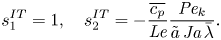(3.6a,b)\begin{equation} s_1^{IT} = 1, \quad s_2^{IT}={-}\frac{\overline{c_p}}{{{Le}}} \frac{{{Pe}_k}}{\tilde{a}\,{{Ja}}\,\bar{\lambda}}. \end{equation}

The rescaled TED-SRT relation, i.e. (2.11), has a singularity at the equilibrium condition so its linearisation is not pursued in this work.

The solution to problem (3.4) can then be derived as

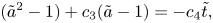(3.7)\begin{equation} ({\tilde{a}}^2-1)+c_3({\tilde{a}}-1)={-}c_4{\tilde{t}}, \end{equation}

where

(3.8a–c)\begin{equation} c_3 = \frac{2(1-s_3^{HK} s_2^{IT}/s_1^{IT})}{(s_1^{HK}+s_2^{HK}\overline{c_p}/Le) {Pe}_0},\quad {Pe}_0 = \frac{u_k a_0}{\mathcal{D}_{AB}}, \quad c_4 = \frac{2\bar{\rho}s_4^{HK}}{s_1^{HK}+s_2^{HK}\overline{c_p}/Le}. \end{equation}

In the large ${Pe}_0$ limit, $c_3$ tends to be zero such that one recovers the classical $D^2$-law. At small ${Pe}_0$, the second linear term becomes dominant so the droplet diameter shrinks linearly with time. The solution for the cases of negligible temperature jump across the Knudsen layer can be found by setting $s_3^{HK}=0$. The lifetime of the droplet $\tau _{HK}$ can be found to be $\tau _{HK}=\tau _{D2}(1+ c_3)$, where $\tau _{D2} = 1/c_4$ is the droplet lifetime assuming local thermodynamic equilibrium. Therefore, the actual lifetime of an evaporating droplet will be longer than the prediction from the classical $D^2$-law due to the kinetic-limited regime towards the end.

3.2. Comparison with experimental data

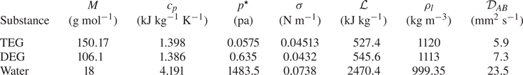
To test the validity of the mixed kinetic-diffusion boundary condition, both the numerical results from the full QS problems and the linearised analytical results are compared with the experimental data reported by Jakubczyk et al. (Reference Jakubczyk, Kolwas, Derkachov, Kolwas and Zientara2012) and Holyst et al. (Reference Holyst, Litniewski, Jakubczyk, Zientara and Woźniak2013b) for the evaporation of triethylene glycol (TEG) and diethylene (DEG) glycol droplets in dry nitrogen and water droplets in humid air. In their experiments, the isolated droplet evaporates very slowly in a nearly isothermal gas domain due to a small gradient in the vapour pressure close to the interface. This enables an accurate time-resolved measurement of the droplet size based on an interferometry technique. Their measurement uncertainty for the droplet size is reported to be up to 10 nm for a single-component droplet (Jakubczyk et al. Reference Jakubczyk, Kolwas, Derkachov, Kolwas and Zientara2012). The physical properties of different fluids and all other parameters used in the model are summarised in table 1. All properties are evaluated from the NIST database (Kroenlein et al. Reference Kroenlein, Muzny, Kazakov, Diky, Chirico, Magee, Abdulagatov and Frenkel2012), except for $\mathcal {D}_{AB}$ (TEG/DEG in dry nitrogen (Lugg Reference Lugg1968); water in air Massman Reference Massman1998) and $p^{\star }$ for TEG and DEG. The saturation pressure $p^{\star }$ at 298 K for both TEG and DEG is very low and no direct experimental data could be found from the literature. Therefore, it was taken as the value leading to the best fit of the measured droplet size, in the region where the classical $D^2$-law is valid, i.e. when the droplet size is sufficiently large so that the kinetic effects are negligibly small (${{Pe}_k} > 30$), and the measurement uncertainty is less than 0.5 %.

Table 1. Physical properties of fluids used in modelling. Both TEG and DEG are evaporated in dry nitrogen at 298 K, 98.7 kPa. Water is evaporated in humid air at 286 K, 99 kPa and 97 relative humidity. The value of $\lambda$ in dry nitrogen and humid air is 66 and 63 nm, respectively (Holyst et al. Reference Holyst, Litniewski, Jakubczyk, Zientara and Woźniak2013b).

The predicted ${\tilde {a}}^2$ and measured ${\tilde {a}}_{{exp}}^2$ and their relative difference, i.e. $({\tilde {a}}_{{exp}}^2-{\tilde {a}}^2)/{\tilde {a}}_{{exp}}^2$, together with the corresponding ${{Pe}_k}$ for the evaporation of a water droplet in humid air are shown in figure 2(a,b). We can clearly see that the classical $D^2$-law (i.e. assuming local thermodynamic equilibrium and ignore surface tension) becomes increasingly inaccurate as the droplet shrinks (i.e. ${{Pe}_k}$ reduces). At large ${{Pe}_k}$, the kinetic process is always much more efficient than the mass diffusion so that the evaporation rate is diffusion limited. However, as the kinetic process becomes less efficient than the mass diffusion for reduced droplet sizes, it becomes the limiting factor and the evaporation rate is decreased. When the surface tension is taken into account, the classical model assuming local thermodynamic equilibrium overestimates the evaporation rate even further, due to the increased saturation pressure at small curvature. Incorporating the mixed kinetic-diffusion boundary conditions with no temperature jump across the Knudsen layer can consistently improve the prediction. However, the extent of improvement is dependent on the magnitude of the temperature jump. When the temperature jump is significant, e.g. evaporation of water in humid air – figure 2(a,b), the improvement is very limited. In contrast, when the temperature jump is small, e.g. evaporation of TEG/DEG in dry nitrogen shown in figure 2(c,d), the improvement is very significant. From figure 2, we can also observe that both accommodation coefficients in (1.1) are very close to 1 when the interface is near equilibrium so that negligible differences are introduced by using the semi-empirical HK correlation with unity accommodation coefficients instead of the more rigorous TED-SRT kinetic model. However, the difference will be larger when the evaporation occurs further away from the equilibrium such that there is a larger temperature jump.

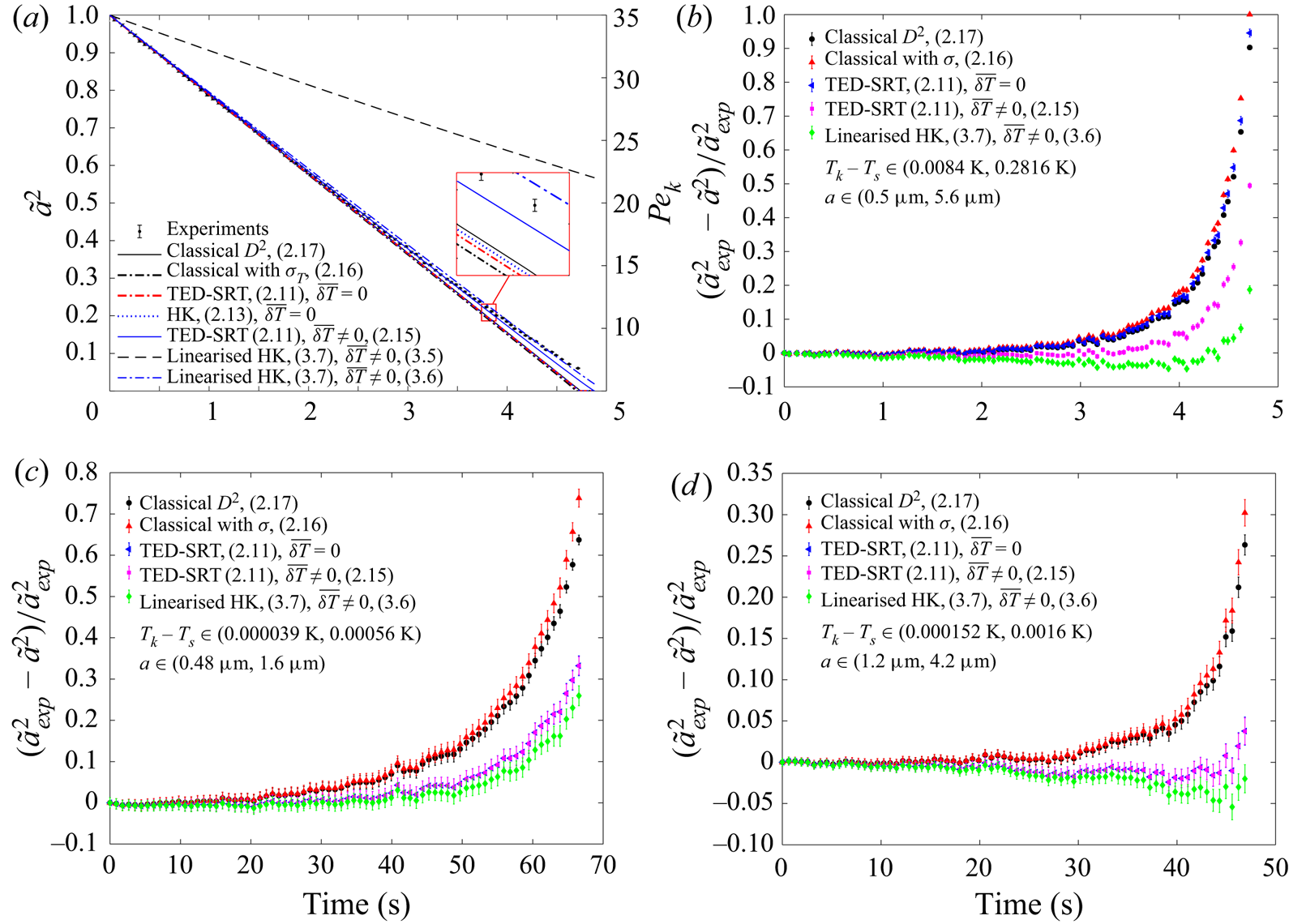
Figure 2. Comparison between the modelled droplet sizes and experimental results. (a,b) Evaporation of a water drop in humid air (experimental data are from Holyst et al. Reference Holyst, Litniewski, Jakubczyk, Zientara and Woźniak2013b). (c) Evaporation of a TEG drop in dry nitrogen (experimental data are from Jakubczyk et al. Reference Jakubczyk, Kolwas, Derkachov, Kolwas and Zientara2012). (d) Evaporation of a DEG drop in dry nitrogen (experimental data are from Holyst et al. Reference Holyst, Litniewski, Jakubczyk, Zientara and Woźniak2013b).

From figure 2(a), we can also see that incorporating the temperature jump model developed for the evaporation of a droplet in its pure vapour (i.e. (2.14)) yields an unrealistically large temperature jump $\overline {\delta T}$ across the Knudsen layer (${\sim }10\ \mathrm {K}$) and consequentially a significantly slower evaporation rate. A closer look to (2.3) suggests that the large value of $\overline {\delta T}$ stems from the very low equilibrium vapour pressure on the liquid surface, i.e. $p_s^{eq}$ and $\overline {\delta T}$ will diverge as $p_s^{eq} \rightarrow 0$, which is not physically acceptable and needs further correction. If the empirical temperature jump model (2.15) is deployed, the QS solution matches the experimental results well in all cases. This good match is a clear indication of the dominant role that the inert gases play in the thermalisation of the vapour molecules emerging from the evaporation. However, the absence of the physical properties of the pure substance (possibly link to the value of $A$) and the heat flux in this empirical correlation means that it does not account for the energy of the emerging vapour molecules properly. The linearised solution, surprisingly, works even better than the full formulation in most cases. This could be an indication that the full formulation needs further revision, possibly through the development of a more rigorous temperature jump model across the Knudsen layer. In summary, among the different models tested, the best option to correct for the error caused by the local thermodynamic equilibrium assumption is to use the mixed kinetic-diffusion boundary condition together with the empirical temperature jump model.

3.3. Parameter domain study

To quantify the potential errors induced by the local thermodynamic equilibrium assumption on the prediction of the evaporation rate, we compared the values of ${{B}_T}$ calculated at different $({{Pe}_k},\varPhi _\infty )$, as shown in figure 3(a). As expected, the error becomes significant when ${{Pe}_k} \leqslant O(10)$ and increases as ${{Pe}_k}$ is further reduced. Figure 3(b) shows that the errors introduced by neglecting the change in liquid surface chemical potential (due to the presence of inert gas) become significant only when $\bar {\rho } \geqslant O(10^{-1})$, which corresponds to high-pressure or low-temperature conditions. Naturally, as one gets closer to the critical point, the ideal gas law breaks down and a more realistic gas model need to be considered.

Figure 3. Comparison of ${{B}_T}$ values calculated at different conditions. Cases of evaporation of a water drop in humid air ignoring the surface tension effect are considered in this calculation: ${{Le}} = 0.8659$, $\overline {c_p}=0.6031$, $\bar {p}=0.01$, ${{Ja}}=0.485$, $\gamma =1.124$, $A = 2.35$, $\lambda = 63$ nm. (a) Percentage error coming from the local thermodynamic equilibrium assumption at different $\{{{Pe}_k},\varPhi _\infty \}$ when $\bar {\rho }=1\times 10^{-3}$; (b) percentage error in ignoring the change of liquid phase chemical potential due to the presence of inert gas at different $\{{{Pe}_k},\bar {\rho }\}$ when $\varPhi _\infty =0.98$.