


1. Introduction
A magnetorheological fluid is a suspension of magnetic particles of size about  $1\unicode{x2013}10\ \mathrm {\mu } {\rm m}$ in a viscous fluid (de Vicente, Klingenberg & Hidalgo-Alvarez Reference de Vicente, Klingenberg and Hidalgo-Alvarez2011; Morillas & de Vicente Reference Morillas and de Vicente2020). Brownian motion is not important in these suspensions, because the particle size exceeds
  $1\ \mathrm {\mu }{\rm m}$, and the viscosity of the carrier fluid could be 2–3 orders of magnitude larger than that of water. The volume fraction of the particles could be as low as
  $10\,\%$ or lower (Anupama, Kumaran & Sahoo Reference Anupama, Kumaran and Sahoo2018). The salient feature of these fluids is the rapid reversible transition between a low-viscosity state in the absence of a magnetic field, where the particles are well dispersed, and a high viscosity state under a magnetic field where the particles form sample-spanning clusters that arrest flow in the conduit (Sherman, Becnel & Wereley Reference Sherman, Becnel and Wereley2015). This transition takes place reversibly and rapidly within time periods of tens to hundreds of milliseconds. Due to this rapid switching, magnetorheological fluids are used in applications such as dampers and shock absorbers (Klingenberg Reference Klingenberg2001).
Magnetorheological fluids are characterised by measuring their ‘yield stress’ as a function of the magnetic field (Sherman et al. Reference Sherman, Becnel and Wereley2015). In the field of rheology, the yield stress for a Bingham plastic fluid delineates solid-like and fluid-like behaviour – the material behaves as an elastic solid when the stress is less than the yield stress, and flows like a viscous liquid when the stress exceeds the yield stress (Barnes, Hutton & Walters Reference Barnes, Hutton and Walters1989). In the Bingham model, the stress is the sum of a yield stress  $\tau _y$ and a contribution that is linear in the strain rate, and the slope of the stress–strain rate curve is called the plastic viscosity. For characterisation, the magnetorheological fluid is placed in a rheometer, and a magnetic field is applied across the sample. The strain rate is then set at progressively increasing values, and the stress is measured. The stress–strain rate curve is fitted to the Bingham plastic model to determine the yield stress and the plastic viscosity. Typically, the stress–strain rate curves for magnetorheological fluids increase continuously, and they do not exhibit a discontinuous change in slope at yield. In order to determine the yield stress and plastic viscosity, the high strain rate behaviour of these fluids is extrapolated linearly to zero strain rate. There are two dimensionless numbers that are used to characterise magnetorheological fluids. The first is the Mason number, the ratio of the shear stress and a reference magnetic stress that is the ratio of the magnetic dipole–dipole interaction force between pairs of particles and the square of the particle diameter (Sherman et al. Reference Sherman, Becnel and Wereley2015). The second is the Bingham number, which is the ratio of the yield stress and the fluid stress. The yield stress does increase as the applied magnetic field is increased, and it has been proposed that the Bingham number is inversely proportional to the Mason number (Sherman et al. Reference Sherman, Becnel and Wereley2015).
More sophisticated constitutive relations for magnetorheological fluids have been explored in simulations and experiments. Empirical fitting functions of the type
 \begin{equation} \frac{\eta}{\eta_0} = 1 + \left( \frac{{Mn}^{{\ast}}}{{Mn}} \right)^{\alpha} \end{equation}
have been used for the effective viscosity  $\eta$, which is the ratio of the stress and strain rate (Vagberg & Tighe Reference Vagberg and Tighe2017). Here,
  $\eta _0$ is the viscosity in the absence of a magnetic field,
  ${Mn}$ is the Mason number, which is proportional to the strain rate, and
  ${Mn}^{\ast }$ and
  $\alpha$ are fitting parameters. Equation (1.1) reduces to the Bingham equation for
  $\alpha = 1$. For
  $\alpha < 1$, there is a transition from a power-law form for the constitutive relation at low
  ${Mn}$ to a Newtonian form for high
  ${Mn}$. While some simulation and experimental studies (Marshall, Zukoski & Goodwin Reference Marshall, Zukoski and Goodwin1989; Bonnecaze & Brady Reference Bonnecaze and Brady1992; Sherman et al. Reference Sherman, Becnel and Wereley2015) on dipolar particles in an external field have found that
  $\alpha$ is close to
  $1$, others (Melrose Reference Melrose1992; Martin, Odinek & Halsey Reference Martin, Odinek and Halsey1994; Felt et al. Reference Felt, Hagenbuchle, Liu and Richard1996) report that the exponent is less than 1. In the simulations of Vagberg & Tighe (Reference Vagberg and Tighe2017), the exponent
  $\alpha$ is found to depend on the details of the interactions between particles. More sophisticated rheological models, such as the Casson model in Ruiz-López, Hidalgo-Alvarez & de Vicente (Reference Ruiz-López, Hidalgo-Alvarez and de Vicente2017), have also been employed for the rheology of magnetorheological fluids.
The above characterisation procedure examines the ‘unjamming’ or dynamical release transition, where the particle structures formed by the magnetic field are disrupted due to shear. However, rapid flow cessation involves the opposite dynamical arrest, where initially dispersed particles cluster and block the flow in the conduit when a magnetic field is applied. The mechanism for dynamical arrest is different from that probed in characterisation experiments. The clustering has to be initiated by interactions between well-dispersed particles upon application of a magnetic field in the presence of flow. Here, some insight is obtained into the initiation of the dynamical arrest process by considering the effect of the hydrodynamic and magnetic interactions between dispersed particles in the sheared state in the presence of a magnetic field.
Ferrofluids (Moskowitz & Rosensweig Reference Moskowitz and Rosensweig1967; Zaitsev & Shliomis Reference Zaitsev and Shliomis1969; Chaves, Zahn & Rinaldi Reference Chaves, Zahn and Rinaldi2008; Schumacher, Riley & Finlayson Reference Schumacher, Riley and Finlayson2008) form another class of suspensions of magnetic particles. In this case, the particles are of nanometre size, Brownian diffusion is significant, and the effect of interactions on the fluctuating motion of the particles may be less important. Suspensions of conducting particles in shear flow also experience a torque in a magnetic field (Moffat Reference Moffat1990; Kumaran Reference Kumaran2019, Reference Kumaran2020b). This is because an eddy current is induced when a particle rotates in a magnetic field, and this induces a magnetic dipole that interacts with the field. Suspensions of conducting particles are not considered here, but a similar calculation procedure can be used to predict the effect of interactions.
Rather than fitting the measured or simulated rheology to a specific constitutive relation, the approach here is to examine the effect of particle interactions in a suspension with well-dispersed particles. This is similar to the effect of particle interactions on the viscosity of a non-Brownian particle suspension (Batchelor Reference Batchelor1970; Hinch Reference Hinch1977). The dynamics of a spheroidal particle subjected to a shear flow and a magnetic field has been studied (Almog & Frankel Reference Almog and Frankel1995; Sobecki et al. Reference Sobecki, Zhang, Zhang and Wang2018; Kumaran Reference Kumaran2020a, Reference Kumaran2021a,Reference Kumaranb). In the absence of a magnetic field, the particle axis rotates in closed ‘Jeffery orbits’ (Hinch & Leal Reference Hinch and Leal1979; Jeffery Reference Jeffery1923) on a unit sphere. When a magnetic field is applied, the magnetic torque tends to align the particle along the field direction. When the magnetic field is below a threshold, the particle rotates with frequency lower than the Jeffery frequency. When the magnetic field exceeds the threshold, the particle has a steady orientation that inclines progressively towards the field direction as the field strength is increased. The transition between steady and rotating states depends on the particle shape factor and the magnetisation model, and there could also be multiple steady states. Here, the effect of interactions is studied for a suspension of spherical particles. Though this configuration is sufficiently simple that the particle orientation can be determined analytically, it does provide physical insight into the mechanisms that drive the collective behaviour of the particles.
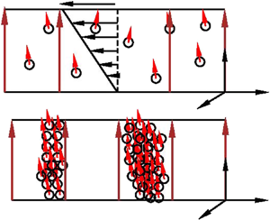
Consider a suspension of spherical magnetic particles sheared between two plates, as shown in figure 1. The effect of any demagnetising field at the boundaries is neglected in the analysis, since we are considering concentration fluctuations in the bulk. The red arrows show the magnetic moment of the particles, and the blue arrows indicate the direction of rotation of the particles due to the fluid shear. When there is no magnetic field, there is no magnetic torque, and the hydrodynamic torque is zero in the viscous limit. The particles rotate with angular velocity equal to the local fluid rotation rate, which is one-half of the vorticity. When a small magnetic field is applied, there is a torque on the particle that depends on the particle orientation. The particles do rotate, but with average angular velocity smaller than the fluid rotation rate, as shown in figure 1(a). When the magnetic field is increased beyond a threshold, the particles do not rotate; the static orientation is determined by a balance between the magnetic and hydrodynamic torques, as shown in figure 1(b). There is a transition between rotating and steady states when the dimensionless parameter  $\varSigma$, defined later in (2.43), exceeds
  $\frac {1}{2}$. In the limit of large magnetic field, the particle magnetic moments align closer to the field direction, as shown in figure 1(c).
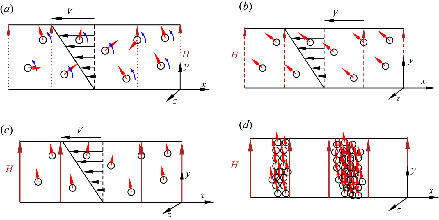
Figure 1. A suspension of dipolar spherical particles in a magnetic field. (a) For low field intensity, the rotation rate is smaller then the fluid rotation rate. (b) Above a threshold, the particles align in the direction determined by a balance between the hydrodynamic and magnetic torques. (c) At high magnetic field, the particles align close to the field direction. (d) Dynamical arrest occurs due to sample-spanning aggregation of particles.
The formation of sample-spanning clusters for dynamical arrest in magnetorheological fluids, shown in figure 1(d), requires an additional mechanism not present in the single-particle dynamics. While alignment of particle dipoles is expected for high magnetic field, it is not clear how the non-Brownian particles approach and cluster in the streamwise direction in a highly viscous fluid where particle contact is prevented by lubrication. Formation of isotropic clusters is not sufficient to explain the dynamical arrest phenomenon; such clusters would be rotated and stretched by the shear flow (Varga et al. Reference Varga, Grenard, Pecorario, Taberlet, Dolique, Manneville, Divoux, McKinley and Swan2019). Here, we show that anisotropic clustering is initiated by interactions between dispersed particles. The interactions are of two types, magnetic and hydrodynamic. It is shown that hydrodynamic interactions between particles amplify concentration variations along the flow direction, while magnetic interactions dampen concentration variations along the cross-stream direction. The amplification of density of waves in the streamwise direction, combined with the rapid equalisation of concentration in the cross-stream direction, could result in the formation of sample-spanning aggregates that arrest the flow.
The effect of magnetic interactions between particles on magnetophoresis has been calculated (Morozov Reference Morozov1993, Reference Morozov1996), and this has been included in models for suspensions of magnetic particles in the presence of magnetic fields (Pshenichnikov, Elfimova & Ivanov Reference Pshenichnikov, Elfimova and Ivanov2011; Pshenichnikov & Ivanov Reference Pshenichnikov and Ivanov2012). Magnetic interactions enhance the diffusion coefficient, dampen concentration and fluctuations, and stabilise the suspension. This is contrary to the aggregation required for dynamical arrest in magnetorheological fluids. The following simple calculation illustrates the diffusion enhancement due to magnetic interactions.
The force on a particle in a magnetic field is assumed to be of the form  ${\boldsymbol {F}} = \mu _0\, \boldsymbol{\nabla } (\boldsymbol{M} \boldsymbol{\cdot } \boldsymbol{H})$, where
  $\mu _0$ is the magnetic permeability (which is considered a constant),
  $\boldsymbol{M}$ is the particle moment, and
  $\boldsymbol{H}$ is the magnetic field. The net force is zero when the magnetic field is uniform in the case of non-interacting particles. The magnetic field disturbance
  $\boldsymbol{H}'(\boldsymbol{x})$ on a particle at the location
  $\boldsymbol{x}$ due to the presence of another particle at the location
  $\boldsymbol{x}'$ with magnetic moment
  $\boldsymbol{M}$ is
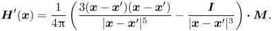 \begin{equation} \boldsymbol{H}'(\boldsymbol{x}) = \frac{1}{4 {\rm \pi}} \left( \frac{3 (\boldsymbol{x} - \boldsymbol{x}')(\boldsymbol{x} - \boldsymbol{x}')}{|\boldsymbol{x} - \boldsymbol{x}'|^{5}} - \frac{\boldsymbol{I}}{|\boldsymbol{x} - \boldsymbol{x}'|^{3}} \right) \boldsymbol{\cdot} \boldsymbol{M}. \end{equation}
In a uniform suspension where the number density is a constant, the integral of the right-hand side of (1.2) over all space is zero by symmetry. In a suspension of particles with a spatially varying number density  $n(\boldsymbol{x})$, the magnetic field at the particle location
  $\boldsymbol{x}$ due to interaction with other particles is
 \begin{equation} \boldsymbol{H}'(\boldsymbol{x}) = \frac{1}{4 {\rm \pi}} \int {\rm d}\kern0.06em \boldsymbol{x}' \left( \frac{3 (\boldsymbol{x} - \boldsymbol{x}')(\boldsymbol{x} - \boldsymbol{x}')}{|\boldsymbol{x} - \boldsymbol{x}'|^{5}} - \frac{\boldsymbol{I}}{|\boldsymbol{x} - \boldsymbol{x}'|^{3}} \right) \boldsymbol{\cdot} (\boldsymbol{M}\,n(\boldsymbol{x}')). \end{equation}
These disturbances are expressed in Fourier space using the transform
 \begin{equation} \hat{\star}_{\boldsymbol{k}} = \int {\rm d}\kern0.06em \boldsymbol{x} \exp{({{\rm{i}}} \boldsymbol{k} \boldsymbol{\cdot} \boldsymbol{x})} \star'(\boldsymbol{x}), \end{equation}
where the field variable  $\star$ could be magnetic field, velocity, vorticity, concentration or the orientation vector. The Fourier transform of the disturbance to the magnetic field is
 \begin{equation} \hat{\boldsymbol{H}}_{\boldsymbol{k}} ={-} \frac{\boldsymbol{k} \boldsymbol{k} \boldsymbol{\cdot} \boldsymbol{M} \hat{n}_{\boldsymbol{k}}}{k^{2}}, \end{equation}
where  $\hat {n}_{\boldsymbol{k}}$ is the Fourier transform of the number density variations. The Fourier transform of the force
  $\boldsymbol{F} = \mu _0\,\boldsymbol{\nabla } (\boldsymbol{M} \boldsymbol{\cdot } \boldsymbol{H})$ acting on the particle is
 \begin{equation} \hat{\boldsymbol{F}}_{\boldsymbol{k}} ={-} {{\rm{i}}} \boldsymbol{k} \mu_0 (\boldsymbol{M} \boldsymbol{\cdot} \hat{\boldsymbol{H}}_{\boldsymbol{k}}) = {{\rm{i}}} \boldsymbol{k} \left( \frac{\mu_0 (\boldsymbol{M} \boldsymbol{\cdot} \boldsymbol{k})(\boldsymbol{M} \boldsymbol{\cdot} \boldsymbol{k}) \hat{n}_{\boldsymbol{k}}}{k^{2}} \right). \end{equation}
The particle velocity drift due to the magnetic interaction force is the ratio of the force and the friction coefficient,
 \begin{equation} \hat{\boldsymbol{u}}_{\boldsymbol{k}} = \frac{\boldsymbol{F}_{\boldsymbol{k}}}{3 {\rm \pi}\eta d} = {{\rm{i}}} \boldsymbol{k} \left( \frac{\mu_0 (\boldsymbol{M} \boldsymbol{\cdot} \boldsymbol{k})(\boldsymbol{M} \boldsymbol{\cdot} \boldsymbol{k}) \hat{n}_{\boldsymbol{k}}}{3 {\rm \pi}\eta {d} k^{2}} \right), \end{equation}
where the Stokes expression for the friction coefficient for a spherical particle,  $3 {\rm \pi}\eta d$, has been used,
  $\eta$ is the fluid viscosity, and
  $d$ is the particle diameter. The variation in number density due to the drift velocity is determined from the conservation equation
 \begin{equation} \frac{\partial \hat{n}_{\boldsymbol{k}}}{\partial t} - {{\rm{i}}} \boldsymbol{k} \boldsymbol{\cdot} (\bar{n} \hat{\boldsymbol{u}}_{\boldsymbol{k}}) = 0. \end{equation}
Here,  $\bar {n}$ is the average number density of the particles, and it is assumed that the variation in number density
  $\hat {n}_{\boldsymbol{k}}$ is much smaller than
  $\bar {n}$. This results in a diffusion-type equation,
 \begin{equation} \frac{\partial \hat{n}_{\boldsymbol{k}}}{\partial t} + \boldsymbol{k} \boldsymbol{k} \boldsymbol{:} ( \boldsymbol{D} \hat{n}_{\boldsymbol{k}}) = 0, \end{equation}
where the diffusion tensor  $\boldsymbol{D}$ is
 \begin{equation} \boldsymbol{D} = \frac{\mu_0 \boldsymbol{M} \boldsymbol{M} \bar{n}}{3 {\rm \pi}\eta d}. \end{equation}
The diffusion tensor depends on the magnetic moment of the particles, and not the magnetic field, because it is caused by the interaction force between the particles, as noted in Sherman et al. (Reference Sherman, Becnel and Wereley2015) and Klingenberg, Ulicny & Golden (Reference Klingenberg, Ulicny and Golden2007). This effect is anisotropic, and it operates only in the direction of the particle moment. Importantly, the effect of interactions dampens fluctuations in the direction of the magnetic moment since the diffusivity is positive, and it has no effect in the direction perpendicular to the particle magnetic moment.
The clustering of particles can be predicted if the variation of the magnetic field due to the magnetic moments of the particles is included in an effective medium approach. The force on the particle is  ${\boldsymbol {F}} = \mu _0\,\boldsymbol{\nabla } [\boldsymbol{M} \boldsymbol{\cdot } (\boldsymbol{H} + n \boldsymbol{M})]$, where
  $n \boldsymbol{M}$ is the magnetisation or the magnetic moment per unit volume. The force on the particles is, instead of (1.6),
 \begin{equation} \hat{\boldsymbol{F}}_{\boldsymbol{k}} ={-} {{\rm{i}}} \boldsymbol{k} \mu_0 (\boldsymbol{M} \boldsymbol{\cdot} \hat{\boldsymbol{H}}_{\boldsymbol{k}} + \hat{n}_{\boldsymbol{k}} \boldsymbol{M} \boldsymbol{\cdot} \boldsymbol{M}) = {{\rm{i}}} \boldsymbol{k} \left( \frac{\mu_0 (\boldsymbol{M} \boldsymbol{\cdot} \boldsymbol{k})(\boldsymbol{M} \boldsymbol{\cdot} \boldsymbol{k}) \hat{n}_{\boldsymbol{k}}}{k^{2}} - M^{2} \hat{n}_{\boldsymbol{k}} \right). \end{equation}
The last term in the bracket on the right arises from the variation in the magnetic moment per unit volume due to the variation in the particle number density. With this inclusion, the diffusion tensor is
 \begin{equation} \boldsymbol{D} = \frac{\mu_0 (\boldsymbol{M} \boldsymbol{M} - \boldsymbol{I} M^{2}) \bar{n}}{3 {\rm \pi}\eta d}, \end{equation}
where  $\boldsymbol{I}$ is the identity tensor. The above diffusion tensor is diagonal in a coordinate system where one of the coordinate directions is along the particle magnetic moment. The diffusion coefficient along the magnetic moment is identically zero, while that in the two directions perpendicular to the magnetic moment is negative. This predicts spontaneous amplification of concentration fluctuations in the direction perpendicular to the magnetic moment of the particles, and no amplification or damping along the particle magnetic moment. This is consistent with the formation of particle chains along the magnetic field direction if the magnetic moment is aligned along the magnetic field. However, this is still an effective medium or a mean-field approach for the initial growth of perturbations.
The contrast in the electrical permittivity or magnetic permeability on the stability of a suspension was considered by von Pfeil et al. (Reference von Pfeil, Graham, Klingenberg and Morris2003) for a sheared particle suspension. In the dilute limit, the effective magnetic permeability is expressed as  $\mu _{eff} = \mu _0 (1 + \mu ^{\prime } \phi )$, where
  $\phi$ is the volume fraction,
  $\mu ^{\prime } = 3 (\mu _R - 1)/(\mu _R + 2)$, with
  $\mu _0$ the magnetic permeability of the fluid in the absence of particles and
  $\mu _R$ the ratio of the magnetic permeabilities of the particles and fluid. For
  $\mu _R > 1$ where the magnetic permeability of the particles is higher than that for the fluid, preferentially the magnetic flux lines pass through regions of higher particle concentration. In the present analysis, the change in the magnetic field due to the particles is the magnetisation or the magnetic moment per unit volume, and the latter is the product of the particle moment and the number density.
When there is fluid flow, there is one other effect, which is the variation in the effective viscosity of the suspension with the particle concentration. For a dilute suspension of spherical particles subject to shear flow, the effective viscosity is  $\eta = (1 + \eta ^{\prime } \phi )$, where
  $\eta ^{\prime } = \frac {5}{2}$ and
  $\phi$ is the volume fraction. The viscosity variation with volume fraction is included in the analysis in §§ 2.1 and 3.1, where an effective diffusion coefficient is derived in the equation for the concentration fluctuation. This effective diffusion coefficient is proportional to
  $\eta ^{\prime }$.
The objective of the present study is to analyse the stability of a flowing suspension incorporating magnetic and hydrodynamic interactions, and the effect of particle concentration on the viscosity and magnetic field. When there is a difference between the particle and fluid rotation rates, there is a torque exerted by the particle on the fluid. This torque results in an antisymmetric dipole force moment at the particle centre, which generates a velocity disturbance. The resulting torque at the centre of a test particle due to interactions with other particles is zero if the number density is uniform (see Appendix D1 in Kumaran Reference Kumaran2019). However, when there is a perturbation in the number density, there is a net torque exerted due to hydrodynamic interactions. In the presence of spatial concentration variations, there is also a net torque exerted at the test particle due to magnetic interactions with other particles. There is a small spatial variation in the particle orientation vector in order to satisfy the zero torque condition. This results in a small correction to the magnetic moment of the particle  $\boldsymbol{M}$, and consequently an additional contribution to the force. The two additional effects of hydrodynamic interactions and the zero torque condition are incorporated in the force due to interactions, and it is shown that this force amplifies concentration fluctuations and destabilises the suspension.
The expression for the force,  $\boldsymbol{F} = \boldsymbol{\nabla } (\boldsymbol{M} \boldsymbol{\cdot } \boldsymbol{B})$, results from the Ampère model for a magnetic dipole, where the dipole is considered as an infinitesimal current loop (Jackson Reference Jackson1975; Griffiths Reference Griffiths2013). Here,
  $\boldsymbol{B} = \mu _0 (\boldsymbol{H} + n \boldsymbol{M})$ is the magnetic flux density. An alternate expression is based on the Gilbert model,
  $\boldsymbol{F} = \boldsymbol{M} \boldsymbol{\cdot } \boldsymbol{\nabla } \boldsymbol{B}$, where the dipole is considered to be the superposition of two magnetic ‘charges’ of opposite signs separated by an infinitesimal distance. Though the two models are equivalent in most cases, there are differences in special situations, such as the magnetic field of a proton that fits the Ampère model. The present analysis is another situation where there are differences in the results of the two models. For small perturbations
  $\boldsymbol{M}'(\boldsymbol{x})$ and
  $\boldsymbol{B}'(\boldsymbol{x})$ about the base state where the particle moment
  $\bar {\boldsymbol{M}}$ and magnetic field
  $\bar {\boldsymbol{B}}$ are spatially uniform, the force in the Gilbert model linearised in the perturbations is
  $\bar {\boldsymbol{M}} \boldsymbol{\cdot } \boldsymbol{\nabla } \boldsymbol{B}'$, whereas that in the Ampère model is
  $\boldsymbol{\nabla } (\boldsymbol{M}'(\boldsymbol{x}) \boldsymbol{\cdot } \bar {\boldsymbol{B}} + \bar {\boldsymbol{M}} \boldsymbol{\cdot } \boldsymbol{B}'(\boldsymbol{x}))$. Variations in the magnetic permeability with position due to a contrast in the permeabilities of the particles and fluid are also incorporated in the Ampère model. The force in the Gilbert model does not depend on the perturbations to the particle magnetic moment, while that in the Ampère model does. Another distinction is that the force in the Ampère model can be written as
  $- \boldsymbol{\nabla } U_M$, where
  $U_M = - \boldsymbol{M} \boldsymbol{\cdot } \boldsymbol{B}$ is the magnetic energy, whereas there is no equivalent relation to an energy for the Gilbert model. Since the Ampère model is also known to fit experimental results, such as the magnetic field of a proton measured in hyperfine splitting of spectral lines (Griffiths Reference Griffiths1982), the Ampère model is used here for the force on the particle.
The analysis is carried out for two magnetisation models, the permanent dipole in § 2, where the magnitude of the magnetic moment is independent of the field, and the induced dipole model in § 3, where the magnitude of the moment is proportional to the component of the magnetic field along the orientation axis. These models have been used earlier to study the single-particle dynamics of a spheroid in a magnetic field (Almog & Frankel Reference Almog and Frankel1995; Sobecki et al. Reference Sobecki, Zhang, Zhang and Wang2018; Kumaran Reference Kumaran2020a, Reference Kumaran2021a,Reference Kumaranb). In the induced dipole model, it is assumed that the magnetic moment of the particle is proportional to the component of the magnetic field along that axis. This model is applicable to superparamagnetic particles, which are usually nanometre-sized single-domain particles polarisable along one axis. Superparamagnetic particles have very little hysteresis, so the constant susceptibility assumption is valid for low magnetic field. This also applies to micron-sized multi-domain ferromagnetic particles, or soft magnets. These are magnetised along an ‘easy axis’ (Rikken et al. Reference Rikken, Nolte, Maan, van Hest, Wilson and Christianen2014) for several reasons. Though the domains within the particles are aligned along the magnetic field for soft magnets, those on the surface are aligned tangential to the surface, resulting in a magnetisation along the particle axis for non-spherical particles. In addition, strain anisotropies could also result in a higher susceptibility along the easy axis. At low magnetic field, this results in a constant anisotropic susceptibility tensor. It was shown Kumaran (Reference Kumaran2021a) that for axisymmetric particles, if the susceptibility is axisymmetric about the easy axis, the magnetic moment can be modelled as a vector directed along the easy axis whose magnitude is proportional to the component of the magnetic field along the easy axis. The induced dipole model used here applies to this case, provided that the magnetic moment is small compared to the saturation moment.
The permanent dipole model applies to particles in ferrofluids, which are suspensions of nanometre-sized single-domain magnetic particles stabilised using surfactants. Here, the orientations of the particles are randomised by Brownian motion in the absence of a magnetic field, but the particles align when a field is applied. The analysis here also applies to superparamagnetic or ferromagnetic particles at high magnetic field when the magnetic moment reaches its saturation value. In contrast to permanent magnets, the magnetic moments align along the component of the field along the easy axis, and magnetic moment reverses when the direction of the field is reversed. Therefore, the orientation dynamics for rotating states is different from that for a permanent magnet (Kumaran Reference Kumaran2020a, Reference Kumaran2021a,Reference Kumaranb). However, for states with a steady orientation that are studied here, the effect of interactions is identical to those for permanent dipolar particles provided that the orientation disturbance is small and it does not reverse the orientation of the magnetic moment.
In addition to dipolar disturbances to the velocity and magnetic field, there are quadrupolar and higher-order disturbances at a test particle due to neighbouring particles. When particles are very close, the lubrication interactions also become important, and there are simultaneous multi-body interactions in a dense suspension. These can be neglected in comparison to the dipolar pair interactions only when the distance between particles is much larger than the particle diameter. This is because the disturbance due to the dipole moment decreases proportional to  $(d/r)^{2}$, that due to the quadrupole moment decreases proportional to
  $(d/r)^{3}$, and that due to the higher terms in the multi-pole expansion decreases proportional to a higher power of
  $(d/r)$, where
  $d$ is the particle diameter and
  $r$ is the distance from the particle centre. Moreover, we have included only pair interactions and neglected simultaneous multi-body interactions. This approximation is also valid in a dilute suspension where the distance between particles is much larger than the particle diameter.
For the permanent and induced dipole models, the dynamics of an isolated spheroid subjected to a shear flow and a magnetic field has been studied (Almog & Frankel Reference Almog and Frankel1995; Sobecki et al. Reference Sobecki, Zhang, Zhang and Wang2018; Kumaran Reference Kumaran2020a, Reference Kumaran2021a,Reference Kumaranb). The results for a spherical particle from these earlier studies are used here. For a permanent dipole, the single-particle dynamics depends on the parameter  $\varSigma$ defined in (2.43), which is the ratio of the magnetic and hydrodynamic torques. The effective diffusion coefficient is calculated in § 2.1, and the rotating and steady states in the absence of particle interactions are summarised in § 2.2. The effect of particle interactions for a parallel magnetic field, where the field is in the flow plane, is discussed in § 2.3, and this is generalised to an oblique magnetic field in § 2.4. The analysis for an induced dipole is provided in § 3, where the single-particle dynamics depends on the parameter
  $\varSigma _i$ defined in (3.19). The diffusion coefficient is calculated in § 3.1, and the calculation of the orientation disturbance of an isolated particle is outlined in § 3.2. The diffusion coefficients for a parallel and oblique magnetic field are provided in §§ 3.3 and 3.4, respectively. In § 4, the major conclusions are summarised, and numerical estimates for the diffusion coefficients are provided.
2. Permanent dipole
A sheared suspension of dipolar particles subject to a magnetic field is considered, where the particle number density is uniform in the base state. The particles have a fixed orientation in the base state due to a balance between the hydrodynamic and magnetic torques. The suspension is considered to be of infinite extent, and demagnetisation at the boundaries is not included.
2.1. Diffusion due to interactions
The magnetic force and torque on a particle with magnetic moment  $\boldsymbol{M}$ in a magnetic field
  $\boldsymbol{H}$ in a suspension of particles with number density
  $n$ are
 \begin{gather} \boldsymbol{F}^{m} = \boldsymbol{\nabla} (\boldsymbol{M} \boldsymbol{\cdot} \mu_0 (\boldsymbol{H} + n \boldsymbol{M})), \end{gather}
 \begin{gather}\boldsymbol{T}^{m} = \mu_0 \boldsymbol{M} \times \boldsymbol{H}, \end{gather}
where  $\mu _0$ is the magnetic permeability. In the expression for the force, (2.1), the magnetic flux density is expressed as
  $\boldsymbol{B} = \mu _0 (\boldsymbol{H} + n \boldsymbol{M})$, where
  $n \boldsymbol{M}$ is the magnetic moment per unit volume. This term is an effective-medium approximation for the variations in the magnetic field due to variations in the number density of particles. The contribution to the magnetic moment per volume in the expression for the torque, (2.2), is zero, since it contains the cross product of the particle moment at a location with itself.
The hydrodynamic force and torque are
 \begin{gather} \boldsymbol{F}^{h} = 3 {\rm \pi}\eta d (\boldsymbol{v} - \boldsymbol{u}), \end{gather}
 \begin{gather}\boldsymbol{T}^{h} = {\rm \pi}\eta d^{3} (\tfrac{1}{2} \boldsymbol{\omega} - \boldsymbol{\varOmega}), \end{gather}
where  $d$ is the particle diameter,
  $\boldsymbol{v}$ and
  $\boldsymbol{\omega }$ are the fluid velocity and vorticity at the particle centre, and
  $\boldsymbol{u}$ and
  $\boldsymbol{\varOmega }$ are the particle linear and angular velocities. The imposed magnetic field is denoted
  $\bar {\boldsymbol{H}}$, and the vorticity due to the imposed shear flow at the particle centre is
  $\bar {\boldsymbol{\omega }}$. The particle magnetic moment is expressed as
  $\boldsymbol{M} = M \boldsymbol{o}$, where
  $M$ is the magnitude of the magnetic moment and
  $\boldsymbol{o}$ is the orientation vector. Linear models are used to incorporate the effect of the variations in the volume fraction on the viscosity and the magnetic permeability,
 \begin{equation} \eta = \eta_0 (1 + \eta^{\prime} \phi^{\prime}), \end{equation}
where  $\phi ^{\prime }=\phi -\bar {\phi }$, with
  $\phi$ the local volume fraction of the particles,
  $\bar {\phi }$ the average volume fraction in the uniform suspension, and
  $\eta _0$ the viscosity for the uniform suspension. For a viscous suspension of spherical particles in the limit of low volume fraction, the result
  $\eta ^{\prime } = \frac {5}{2}$ is obtained for the Einstein correction to the viscosity.
The orientation vector of the particle  $\boldsymbol{o}$ is determined from the torque balance equation,
  $\boldsymbol{T}^{m} + \boldsymbol{T}^{h} = 0$:
 \begin{equation} {\rm \pi}\eta d^{3} (\tfrac{1}{2} \boldsymbol{\omega} - \boldsymbol{\varOmega}) + \mu_0 M (\boldsymbol{o} \times \boldsymbol{H}) = 0. \end{equation}
The magnetic force on the particle (2.1) is zero in a uniform suspension. The force balance requires that the hydrodynamic force is also zero, that is, the particle moves with the same velocity as the fluid,  $\bar {\boldsymbol{u}} = \bar {\boldsymbol{v}}$.
For a stable stationary state where the particle orientation is steady, the component of the angular velocity  $\boldsymbol{\varOmega }$ perpendicular to the orientation vector is zero. However, the particle does spin around the orientation vector, and the components of the particle angular velocity and fluid rotation rate (one-half of the vorticity) along the orientation vector are equal. This is because the torque exerted by the magnetic field is perpendicular to the direction of the magnetic moment and the magnetic field, and consequently there is no magnetic torque along the orientation vector. Therefore, the particle angular velocity is necessarily along the orientation vector,
  $\boldsymbol{\varOmega } = \varOmega \boldsymbol{o}$. It is necessary to consider the torque balance equations parallel and perpendicular to the orientation vector in order to determine the particle orientation. The torque balance equation along the orientation vector is obtained by taking the dot product of (2.6) with
  $\boldsymbol{o}$, and this is solved to obtain
 \begin{equation} \varOmega = \tfrac{1}{2} \boldsymbol{\omega} \boldsymbol{\cdot} \boldsymbol{o}. \end{equation}
The above solution (2.7) for the angular velocity is substituted into the torque balance equation (2.6) to obtain
 \begin{equation} \tfrac{1}{2} {\rm \pi}\eta d^{3} (\boldsymbol{I} - \boldsymbol{o} \boldsymbol{o}) \boldsymbol{\cdot} \boldsymbol{\omega} + \mu_0 M (\boldsymbol{o} \times \boldsymbol{H}) = 0, \end{equation}
where  $\boldsymbol{I}$ is the identity tensor, and
  $(\boldsymbol{I} - \boldsymbol{o} \boldsymbol{o}) \boldsymbol {\cdot }$ is the transverse projection operator that projects a vector on to the plane perpendicular to
  $\boldsymbol{o}$. One relation between the vorticity, magnetic field and orientation vector is obtained by taking the dot product of (2.8) with
  $\boldsymbol{H}$:
 \begin{equation} \boldsymbol{H} \boldsymbol{\cdot} \boldsymbol{\omega} - (\boldsymbol{o} \boldsymbol{\cdot} \boldsymbol{H})(\boldsymbol{o} \boldsymbol{\cdot} \boldsymbol{\omega}) = 0. \end{equation}
The torque balance for the base state in the absence of interactions is obtained by substituting  $\bar {\boldsymbol{o}}$,
  $\bar {\boldsymbol{\omega }}$ and
  $\bar {\boldsymbol{H}}$ for
  $\boldsymbol{o}$,
  $\boldsymbol{\omega }$ and
  $\boldsymbol{H}$ in (2.8).
There is a disturbance to the magnetic field  $\boldsymbol{H}'$ and the fluid vorticity
  $\boldsymbol{\omega }'$ due to a number density fluctuation
  ${n'}(\boldsymbol{x})$ imposed on a uniform suspension with number density
  $\bar {n}$. The orientation vector of the particle is expressed as
  $\boldsymbol{o} = \bar {\boldsymbol{o}} + \boldsymbol{o}'(\boldsymbol{x})$, where
  $\boldsymbol{o}'(\boldsymbol{x})$ is the disturbance to the orientation vector due to hydrodynamic and magnetic interactions resulting from concentration inhomogeneities; the latter is calculated from the torque balance equation. In the linear approximation where terms quadratic in the primed quantities are neglected, the mean and disturbance to the orientation vector satisfy
 \begin{equation} |\bar{\boldsymbol{o}}| = 1, \quad \bar{\boldsymbol{o}} \boldsymbol{\cdot} \boldsymbol{o}' = 0. \end{equation}
The reason for the above relations is that both  $\bar {\boldsymbol{o}}$ and
  $(\bar {\boldsymbol{o}} + \boldsymbol{o}')$ are unit vectors, that is,
  $\bar {\boldsymbol{o}} \boldsymbol{\cdot } \bar {\boldsymbol{o}} = 1$ and
  $(\bar {\boldsymbol{o}} + \boldsymbol{o}') \boldsymbol{\cdot } (\bar {\boldsymbol{o}} + \boldsymbol{o}') = 1$. In the linear approximation, this implies that
  $(\bar {\boldsymbol{o}} \boldsymbol{\cdot } \bar {\boldsymbol{o}} + 2 \bar {\boldsymbol{o}} \boldsymbol{\cdot } \boldsymbol{o}') = 1$. Therefore,
  $\bar {\boldsymbol{o}} \boldsymbol{\cdot } \boldsymbol{o}' = 0$.
The Fourier transform  $\hat {\boldsymbol{o}}_{\boldsymbol{k}}$ of the disturbance to the orientation vector is defined using (1.4). The Fourier transform of the force on a particle due to interactions is determined from (2.1) as
 \begin{equation} \hat{\boldsymbol{F}}_{\boldsymbol{k}} ={-} {{\rm{i}}} \boldsymbol{k} \mu_0 M [\bar{\boldsymbol{o}} \boldsymbol{\cdot} \hat{\boldsymbol{H}}_{\boldsymbol{k}} + \bar{\boldsymbol{H}} \boldsymbol{\cdot} \hat{\boldsymbol{o}}_{\boldsymbol{k}} + M \hat{n}_{\boldsymbol{k}}], \end{equation}
where  $M$ is the magnitude of the magnetic moment. The last term in the square brackets on the right in (2.11) is the force due to the variation in the number density in the expression (2.1).
The conservation equation for the particle number density is
 \begin{equation} \frac{\partial n}{\partial t} + \boldsymbol{\nabla} \boldsymbol{\cdot} (\boldsymbol{u} n) = D_B\,\nabla^{2} n, \end{equation}
where  $\boldsymbol{u}$ is the particle velocity and
  $D_B$ is the Brownian diffusion coefficient. The particle velocity is expressed as the sum of the fluid velocity
  $\boldsymbol{v}$ and the particle velocity relative to the fluid,
  $(\boldsymbol{u} - \boldsymbol{v}) + \boldsymbol{v}$. Since there is no net force on the particles in a uniform suspension,
  $\bar {\boldsymbol{u}} = \bar {\boldsymbol{v}}$. In the linear approximation, the particle conservation equation is expressed as
 \begin{equation} \frac{\partial {n'}}{\partial t} + \boldsymbol{\nabla} \boldsymbol{\cdot} (\bar{\boldsymbol{v}} {n'} + \boldsymbol{v}^{\prime} \bar{n}) + \boldsymbol{\nabla} \boldsymbol{\cdot} ((\boldsymbol{u}^{\prime} -\boldsymbol{v}^{\prime}) \bar{n}) = D_B\,\nabla^{2} n. \end{equation}
The Fourier transform of the above equation is
 \begin{equation} \frac{\partial \hat{n}_{\boldsymbol{k}}}{\partial t} - {{\rm{i}}} \boldsymbol{k} \boldsymbol{\cdot} (\bar{\boldsymbol{v}} \hat{n}_{\boldsymbol{k}}) - {{\rm{i}}} \boldsymbol{k} \boldsymbol{\cdot} (\bar{n} \hat{\boldsymbol{v}}_{\boldsymbol{k}}) - {{\rm{i}}} \boldsymbol{k} \bar{n} (\hat{\boldsymbol{u}}_{\boldsymbol{k}} - \hat{\boldsymbol{v}}_{\boldsymbol{k}}) + D_B k^{2} \hat{n}_{\boldsymbol{k}} = 0. \end{equation}
The first two terms on the left of (2.14) are the rate of change and the convection of concentration fluctuations due to the base flow. The third term on the left is the rate of change of concentration disturbances due to fluid velocity perturbation. The perturbation to the fluid velocity at a test particle due to the rotation of neighbouring particles, which is calculated later in (2.22), is perpendicular to  $\boldsymbol{k}$. Consequently, the third term on the left in (2.14) is zero. The fourth term on the left is the relative motion between the particles and the fluid due to the forces on the particle.
In a dilute suspension, the difference between the particle and fluid velocity disturbances,  $\hat {\boldsymbol{u}}_{\boldsymbol{k}}$ and
  $\hat {\boldsymbol{v}}_{\boldsymbol{k}}$, is given by Stokes’ law,
 \begin{equation} \hat{\boldsymbol{u}}_{\boldsymbol{k}} - \hat{\boldsymbol{v}}_{\boldsymbol{k}} = \frac{\hat{\boldsymbol{F}}_{\boldsymbol{k}}}{3 {\rm \pi}\eta_0 d}. \end{equation}
The drift velocity does not depend on the coefficient  $\eta ^{\prime }$ in (2.5) in the linear approximation, because the force on a particle is zero in a uniform suspension.
The expression (2.15) for the drift velocity is substituted into the linearised conservation equation (2.14):
 \begin{equation} \frac{\partial \hat{n}_{\boldsymbol{k}}}{\partial t} - {{\rm{i}}} \boldsymbol{k} \boldsymbol{\cdot} (\hat{n}_{\boldsymbol{k}} \bar{\boldsymbol{v}}) + D_B k^{2} \hat{n}_{\boldsymbol{k}} - \frac{k^{2} \bar{n} \mu_0 M (\bar{\boldsymbol{o}} \boldsymbol{\cdot} \hat{\boldsymbol{H}}_{\boldsymbol{k}} + \bar{\boldsymbol{H}} \boldsymbol{\cdot} \hat{\boldsymbol{o}}_{\boldsymbol{k}} + M \hat{n}_{\boldsymbol{k}})}{3 {\rm \pi}\eta_0 d} = 0. \end{equation}
The disturbance  $\hat {\boldsymbol{H}}_{\boldsymbol{k}}$ due to magnetic interactions is expressed as a function of
  $\hat {n}_{\boldsymbol{k}}$, and the orientation disturbance
  $\hat {\boldsymbol{o}}_{\boldsymbol{k}}$, currently unknown, is determined from the first correction to the torque balance. These are substituted into (2.16) to obtain an equation of the form
 \begin{equation} \frac{\partial \hat{n}_{\boldsymbol{k}}}{\partial t} - {{\rm{i}}} \boldsymbol{k} \boldsymbol{\cdot} (\hat{n}_{\boldsymbol{k}} \bar{\boldsymbol{u}}) + \boldsymbol{k} \boldsymbol{\cdot} \boldsymbol{D} \boldsymbol{\cdot} \boldsymbol{k} \hat{n}_{\boldsymbol{k}} + D_B k^{2} \hat{n}_{\boldsymbol{k}} = 0, \end{equation}
where  $\boldsymbol{D}$ is the magnetophoretic diffusion tensor due to hydrodynamic and magnetic interactions. In the following calculation, first the disturbances to the magnetic field and the vorticity due to particle interactions are discussed, and then the disturbance to the orientation vector is calculated using torque balance. This is inserted into (2.16) to extract the diffusion tensor
  $\boldsymbol{D}$.
The change in the magnetic field at the location  $\boldsymbol{x}$ due to interactions with other particles is a generalisation of (1.3) which incorporates the disturbance to the orientation vector,
 \begin{equation} \boldsymbol{H}'(\boldsymbol{x}) = \frac{1}{4 {\rm \pi}} \int {\rm d}\kern0.06em \boldsymbol{x}' \left( \frac{3 (\boldsymbol{x} - \boldsymbol{x}')(\boldsymbol{x} - \boldsymbol{x}')}{|\boldsymbol{x} - \boldsymbol{x}'|^{5}} - \frac{\boldsymbol{I}}{|\boldsymbol{x} - \boldsymbol{x}'|^{3}} \right) \boldsymbol{\cdot} [M (\bar{\boldsymbol{o}} {n'}(\boldsymbol{x}') + \bar{n} \boldsymbol{o}'(\boldsymbol{x}'))], \end{equation}
where  ${\rm d}\boldsymbol{x}'$ is the volume element. It is easily verified that the contribution to
  $\boldsymbol{H}'$ due to the product of the background constant particle density and magnetic field,
  $M \bar {n} \bar {\boldsymbol{o}}$, is zero. Equation (1.4) is used to determine the disturbance to magnetic field in reciprocal space,
 \begin{equation} \hat{\boldsymbol{H}}_{\boldsymbol{k}} ={-} \frac{\boldsymbol{k} \boldsymbol{k} \boldsymbol{\cdot} [M (\bar{\boldsymbol{o}} \hat{n}_{\boldsymbol{k}} + \bar{n} \hat{\boldsymbol{o}}_{\boldsymbol{k}})]}{k^{2}} = \hat{\boldsymbol{H}}'_{\boldsymbol{k}} + \hat{\boldsymbol{H}}''_{\boldsymbol{k}} \boldsymbol{\cdot} \hat{\boldsymbol{o}}_{\boldsymbol{k}}, \end{equation}
where
 \begin{equation} \hat{\boldsymbol{H}}'_{\boldsymbol{k}} ={-} \frac{M \hat{n}_{\boldsymbol{k}} \boldsymbol{k} \boldsymbol{k} \boldsymbol{\cdot} \bar{\boldsymbol{o}}}{k^{2}}, \quad\hat{\boldsymbol{H}}''_{\boldsymbol{k}} ={-} \frac{M \bar{n} \boldsymbol{k} \boldsymbol{k}}{k^{2}}.\end{equation}
Note that  $\hat {\boldsymbol{H}}'_{\boldsymbol{k}}$ is a vector, and
  $\hat {\boldsymbol{H}}''_{\boldsymbol{k}}$ is a second-order tensor.
For a particle located at  $\boldsymbol{x}'$ in a fluid with vorticity
  $\bar {\boldsymbol{\omega }}$ in the absence of the particle, the fluid velocity disturbance
  $\boldsymbol{v}'$ at the location
  $\boldsymbol{x}$ is
 \begin{align} \boldsymbol{v}'(\boldsymbol{x}) & = \int {\rm d}\kern0.06em \boldsymbol{x}'\, n(\boldsymbol{x}') \left(\varOmega(\boldsymbol{x}') - \frac{1}{2} \boldsymbol{\omega}(\boldsymbol{x}')\right) \times \frac{d^{3} (\boldsymbol{x} - \boldsymbol{x}')}{8 |\boldsymbol{x} - \boldsymbol{x}'|^{3}} \nonumber\\ & ={-} \int {\rm d}\kern0.06em \boldsymbol{x}' \,n(\boldsymbol{x}') [\boldsymbol{I} - \boldsymbol{o}(\boldsymbol{x}')\,\boldsymbol{o}(\boldsymbol{x}')] \boldsymbol{\cdot} \boldsymbol{\omega}(\boldsymbol{x}') \times \frac{d^{3} (\boldsymbol{x} - \boldsymbol{x}')}{16 |\boldsymbol{x} - \boldsymbol{x}'|^{3}} \nonumber\\ & ={-} \int {\rm d}\kern0.06em \boldsymbol{x}' [ {n'}(\boldsymbol{x}')\,(\boldsymbol{I} - \bar{\boldsymbol{o}} \bar{\boldsymbol{o}}) \boldsymbol{\cdot} \bar{\boldsymbol{\omega}} + \bar{n} (\boldsymbol{I} - \bar{\boldsymbol{o}} \bar{\boldsymbol{o}}) \boldsymbol{\cdot} \boldsymbol{\omega}'(\boldsymbol{x}') \nonumber\\ & \quad - \bar{n} (\bar{\boldsymbol{o}} \bar{\boldsymbol{\omega}} + \boldsymbol{I} \bar{\boldsymbol{\omega}} \boldsymbol{\cdot} \bar{\boldsymbol{o}}) \boldsymbol{\cdot} \boldsymbol{o}'(\boldsymbol{x}')] \times \frac{d^{3} (\boldsymbol{x} - \boldsymbol{x}')}{16 |\boldsymbol{x} - \boldsymbol{x}'|^{3}}. \end{align}
The expression (2.7) for the particle angular velocity has been used to simplify in the second step in (2.21). The linearisation approximation has been used in the third step in (2.21), resulting in an equation that is linear in the disturbances due to particle interactions. The Fourier transform of the velocity field is
 \begin{equation} \hat{\boldsymbol{v}}_{\boldsymbol{k}} ={-} [\hat{n}_{\boldsymbol{k}} (\boldsymbol{I} - \bar{\boldsymbol{o}} \bar{\boldsymbol{o}}) \boldsymbol{\cdot} \bar{\boldsymbol{\omega}} + \bar{n} (\boldsymbol{I} - \bar{\boldsymbol{o}} \bar{\boldsymbol{o}}) \boldsymbol{\cdot} \hat{\boldsymbol{\omega}}_{\boldsymbol{k}} - \bar{n} \hat{\boldsymbol{o}}_{\boldsymbol{k}} \boldsymbol{\cdot} (\bar{\boldsymbol{\omega}} \bar{\boldsymbol{o}} + {\boldsymbol{I}} \bar{\boldsymbol{\omega}} \boldsymbol{\cdot} \bar{\boldsymbol{o}})] \times \frac{{\rm \pi} {d}^{3} {{\rm{i}}} \boldsymbol{k}}{4 k^{2}}. \end{equation}
The Fourier transform of the disturbance to the fluid vorticity is
 \begin{align} \hat{\boldsymbol{\omega}}_{\boldsymbol{k}} & ={-} {{\rm{i}}} \boldsymbol{k} \times \hat{\boldsymbol{v}}_{\boldsymbol{k}} \nonumber\\ & = \frac{{\rm \pi} {d}^{3} (\boldsymbol{k} \boldsymbol{k} - \boldsymbol{I} k^{2}) \boldsymbol{\cdot} [\hat{n}_{\boldsymbol{k}} (\boldsymbol{I} - \bar{\boldsymbol{o}} \bar{\boldsymbol{o}}) \boldsymbol{\cdot} \bar{\boldsymbol{\omega}} + \bar{n} (\boldsymbol{I} - \bar{\boldsymbol{o}} \bar{\boldsymbol{o}}) \boldsymbol{\cdot} \hat{\boldsymbol{\omega}}_{\boldsymbol{k}} - \bar{n} (\bar{\boldsymbol{o}} \bar{\boldsymbol{\omega}} + {\boldsymbol{I}} \bar{\boldsymbol{\omega}} \boldsymbol{\cdot} \bar{\boldsymbol{o}}) \boldsymbol{\cdot} \hat{\boldsymbol{o}}_{\boldsymbol{k}}]}{4 k^{2}}. \end{align}
The above implicit equation is solved for  $\hat {\boldsymbol{\omega }}_{\boldsymbol{k}}$:
 \begin{equation} \left( \boldsymbol{I} - \frac{{\rm \pi} {d}^{3} \bar{n} (\boldsymbol{k} \boldsymbol{k} - \boldsymbol{I} k^{2}) \boldsymbol{\cdot} (\boldsymbol{I} - \bar{\boldsymbol{o}} \bar{\boldsymbol{o}})}{4 k^{2}} \right) \boldsymbol{\cdot} \hat{\boldsymbol{\omega}}_{\boldsymbol{k}} = \hat{\boldsymbol{\omega}}' + \hat{\boldsymbol{\omega}}'' \boldsymbol{\cdot} \hat{\boldsymbol{o}}_{\boldsymbol{k}}, \end{equation}
where
 \begin{gather} \hat{\boldsymbol{\omega}}' = \frac{{\rm \pi} \hat{n}_{\boldsymbol{k}} {d}^{3} (\boldsymbol{k} \boldsymbol{k} - \boldsymbol{I} k^{2}) \boldsymbol{\cdot} (\boldsymbol{I} - \bar{\boldsymbol{o}} \bar{\boldsymbol{o}}) \boldsymbol{\cdot} \bar{\boldsymbol{\omega}}}{4 k^{2}}, \end{gather}
 \begin{gather}\hat{\boldsymbol{\omega}}'' ={-} \frac{{\rm \pi} \bar{n} d^{3} (\boldsymbol{k} \boldsymbol{k} - \boldsymbol{I} k^{2}) \boldsymbol{\cdot} (\bar{\boldsymbol{o}} \bar{\boldsymbol{\omega}} + \boldsymbol{I} \bar{\boldsymbol{\omega}} \boldsymbol{\cdot} \bar{\boldsymbol{o}})}{4 k^{2}}. \end{gather}
Note that  $\hat {\boldsymbol{\omega }}'_{\boldsymbol{k}}$ is a vector, and
  $\hat {\boldsymbol{\omega }}''_{\boldsymbol{k}}$ is a second-order tensor. The latter is proportional to
  ${d}^{3} \bar {n}$ or the volume fraction. In the limit of small volume fraction, this term is small compared to
  $1$.
$1$.
The velocity due to the force exerted by particles is higher order in gradients or higher power in  $\boldsymbol{k}$, so it will result in a higher gradient of the concentration field. The contribution to the velocity due to the magnetic field perturbation, in Fourier space, is
  $|\hat {\boldsymbol{F}}_{\boldsymbol{k}}|/ 3 {\rm \pi}\eta d \sim k \mu _0 M \hat {\boldsymbol{H}}_{\boldsymbol{k}}/3 {\rm \pi}\eta d \sim k \mu _0 M^{2} \hat {n}_{\boldsymbol{k}}/3 {\rm \pi}\eta d$, where
  $k$ is the magnitude of the wavenumber. Here, (2.11) is used for the force, and (2.19), (2.20a,b) are used for the magnetic field perturbation. The magnitude of the fluid velocity due to particle rotation, from (2.22), is
  $|\hat {\boldsymbol{v}}_{\boldsymbol{k}}| \sim {\rm \pi}|\bar {\boldsymbol{\omega }}| \hat {n}_{\boldsymbol{k}} {d}^{3}/k$. The ratio of the velocities due to the force and torque is
  $k^{2} \mu _0 M^{2}/3 {\rm \pi}\eta {d}^{4} |\bar {\boldsymbol{\omega }}| \sim (k d)^{2} {M^{\ast }} \varSigma$, where the dimensionless groups
  $\varSigma$ and
  ${M^{\ast }}$ are defined later, in (2.43) and (2.44). The continuum approximation is valid only for
  $k d \ll 1$; that is, the length scale for the gradients in the concentration field is much larger than the particle diameter. In this limit, the velocity disturbance due to the particle force is neglected compared to that due to the torque exerted on the fluid.
The disturbance to the magnetic field and the vorticity at the particle location causes a disturbance to the particle orientation  $\boldsymbol{o}$, which is determined from the correction to the torque balance equation in Fourier space. The torque balance equation, (2.8), is divided by
  $\mu _0 M$ and linearised in the primed quantities to obtain
 \begin{align} &\frac{{\rm \pi} d^{3} \eta_0}{2 \mu_0 M}\,[(\boldsymbol{I} - \bar{\boldsymbol{o}} \bar{\boldsymbol{o}}) \boldsymbol{\cdot} \hat{\boldsymbol{\omega}}_{\boldsymbol{k}} - \bar{\boldsymbol{o}} (\hat{\boldsymbol{o}}_{\boldsymbol{k}} \boldsymbol{\cdot} \bar{\boldsymbol{\omega}}) - \hat{\boldsymbol{o}}_{\boldsymbol{k}} (\bar{\boldsymbol{o}} \boldsymbol{\cdot} \bar{\boldsymbol{\omega}}) + \eta^{\prime} \hat{\phi}_{\boldsymbol{k}} (\boldsymbol{I} - \bar{\boldsymbol{o}} \bar{\boldsymbol{o}}) \boldsymbol{\cdot} \bar{\boldsymbol{\omega}}] & \nonumber\\ &\quad + (\bar{\boldsymbol{o}} \times \hat{\boldsymbol{H}}_{\boldsymbol{k}} + \hat{\boldsymbol{o}}_{\boldsymbol{k}} \times \bar{\boldsymbol{H}}) = 0, \end{align}
where  $\hat {\phi }_{\boldsymbol{k}} = \hat {n}_{\boldsymbol{k}} ({\rm \pi} d^{3}/6)$ is the Fourier transform of the fluctuation in the volume fraction. The expressions (2.19) and (2.24) for
  $\hat {\boldsymbol{H}}_{\boldsymbol{k}}$ and
  $\hat {\boldsymbol{\omega }}_{\boldsymbol{k}}$ are substituted into (2.27):
 \begin{align} &\frac{{\rm \pi} d^{3} \eta_0}{2 \mu_0 M}\,\{(\boldsymbol{I} - \bar{\boldsymbol{o}} \bar{\boldsymbol{o}}) \boldsymbol{\cdot} \hat{\boldsymbol{\omega}}'_{\boldsymbol{k}} + [(\boldsymbol{I} - \bar{\boldsymbol{o}} \bar{\boldsymbol{o}}) \boldsymbol{\cdot} \hat{\boldsymbol{\omega}}''_{\boldsymbol{k}} - \bar{\boldsymbol{o}} \bar{\boldsymbol{\omega}} - (\bar{\boldsymbol{o}} \boldsymbol{\cdot} \bar{\boldsymbol{\omega}}) \boldsymbol{I}] \boldsymbol{\cdot} \hat{\boldsymbol{o}}_{\boldsymbol{k}} \nonumber\\ &\quad + \eta^{\prime} \hat{\phi}_{\boldsymbol{k}} (\boldsymbol{I} - \bar{\boldsymbol{o}} \bar{\boldsymbol{o}}) \boldsymbol{\cdot} \bar{\boldsymbol{\omega}} \} + [\bar{\boldsymbol{o}} \times \hat{\boldsymbol{H}}'_{\boldsymbol{k}} + \hat{\boldsymbol{o}}_{\boldsymbol{k}} \times \bar{\boldsymbol{H}} + \bar{\boldsymbol{o}} \times (\hat{\boldsymbol{H}}''_{\boldsymbol{k}} \boldsymbol{\cdot} \hat{\boldsymbol{o}}_{\boldsymbol{k}})] = 0. \end{align}
The first term on the left-hand side of (2.28) is the correction to the hydrodynamic torque due to interactions and due to the concentration dependence of the viscosity and magnetic permeability. In this, the contribution proportional to  $\eta ^{\prime } \hat {\phi }_{\boldsymbol{k}}$ is the correction to the hydrodynamic torque due to the concentration dependence of the viscosity. In the first term on the left in (2.28), within the braces, the prefactor of
  $\hat {\boldsymbol{o}}_{\boldsymbol{k}}$ contains one contribution proportional to
  $\hat {\boldsymbol{\omega }}''$, and a second that is proportional to
  $|\bar {\boldsymbol{\omega }}|$. From (2.26), the former is proportional to
  $\bar {n} d^{3} |\bar {\boldsymbol{\omega }}|$, which is small compared to the latter, because the volume fraction is small. Therefore, the term
  $(\boldsymbol{I} - \bar {\boldsymbol{o}} \bar {\boldsymbol{o}}) \boldsymbol{\cdot } \hat {\boldsymbol{\omega }}''_{\boldsymbol{k}}$ is neglected in the first term on the left in (2.28). The second term on the left in (2.28) is the contribution due to the magnetic torque. There are two terms containing
  $\hat {\boldsymbol{o}}_{\boldsymbol{k}}$ in the magnetic torque, the first proportional to
  $|\bar {\boldsymbol{H}}|$ and the second proportional to
  $|\hat {\boldsymbol{H}}''_{\boldsymbol{k}}|$. From (2.20a,b), the latter scales as
  $\bar {n} M$, where
  $M$ is the magnetic moment of a particle. From dimensional analysis,
  $\bar {n} M$ is the disturbance to the magnetic field at a distance
  $\bar {n}^{-1/3}$ from a particle, comparable to the inter-particle distance in the suspension. The weak interaction limit is considered here, where the magnetic field disturbance due to particle interactions is small compared to the applied field,
  $\bar {n} M \ll |\bar {\boldsymbol{H}}|$. Therefore, the term containing
  $\bar {\boldsymbol{o}} \times (\hat {\boldsymbol{H}}''_{\boldsymbol{k}} \boldsymbol{\cdot } \hat {\boldsymbol{o}}_{\boldsymbol{k}})$ is neglected in comparison to
  $\hat {\boldsymbol{o}}_{\boldsymbol{k}} \times \bar {\boldsymbol{H}}$ in (2.28).
Equation (2.28) is solved to obtain the unknown orientation disturbance  $\hat {\boldsymbol{o}}_{\boldsymbol{k}}$. Since
  $\hat {\boldsymbol{o}}_{\boldsymbol{k}}$ is perpendicular to
  $\bar {\boldsymbol{o}}$ from (2.10a,b),
  $\hat {\boldsymbol{o}}_{\boldsymbol{k}}$ is expressed as
 \begin{equation} \hat{\boldsymbol{o}}_{\boldsymbol{k}} = \hat{o}^{{{\dagger}}}_{\boldsymbol{k}} (\bar{\boldsymbol{H}} - (\bar{\boldsymbol{o}} \boldsymbol{\cdot} \bar{\boldsymbol{H}}) \bar{\boldsymbol{o}}) + \hat{o}^{\ddagger}_{\boldsymbol{k}} (\bar{\boldsymbol{o}} \times \bar{\boldsymbol{H}}), \end{equation}
where  $\hat {o}^{{{\dagger}} }_{\boldsymbol{k}}$ and
  $\hat {o}^{\ddagger }_{\boldsymbol{k}}$ are scalar functions of the wavenumber. The specific form (2.29) is chosen because it satisfies the requirement
  $\hat {\boldsymbol{o}}_{\boldsymbol{k}} \boldsymbol{\cdot } \bar {\boldsymbol{o}} = 0$. The expression (2.29) is inserted into the torque balance equation (2.28):
 \begin{align} &\frac{{\rm \pi} d^{3} \eta_0}{2 \mu_0 M}\,\{(\boldsymbol{I} - \bar{\boldsymbol{o}} \bar{\boldsymbol{o}}) \boldsymbol{\cdot} \hat{\boldsymbol{\omega}}'_{\boldsymbol{k}} - \bar{\boldsymbol{o}} [\hat{o}^{{{\dagger}}}_{\boldsymbol{k}} \underline{(\bar{\boldsymbol{H}} - (\bar{\boldsymbol{o}} \boldsymbol{\cdot} \bar{\boldsymbol{H}}) \bar{\boldsymbol{o}}) \boldsymbol{\cdot} \bar{\boldsymbol{\omega}}} + \hat{o}^{\ddagger}_{\boldsymbol{k}} (\bar{\boldsymbol{o}} \times \bar{\boldsymbol{H}}) \boldsymbol{\cdot} \bar{\boldsymbol{\omega}}] \nonumber\\ &\quad - (\bar{\boldsymbol{o}} \boldsymbol{\cdot} \bar{\boldsymbol{\omega}}) [\hat{o}^{{{\dagger}}}_{\boldsymbol{k}} (\bar{\boldsymbol{H}} - (\bar{\boldsymbol{o}} \boldsymbol{\cdot} \bar{\boldsymbol{H}}) \bar{\boldsymbol{o}}) + \hat{o}^{\ddagger}_{\boldsymbol{k}} (\bar{\boldsymbol{o}} \times \bar{\boldsymbol{H}})] + \eta^{\prime} \hat{\phi}_{\boldsymbol{k}} (\boldsymbol{I} - \bar{\boldsymbol{o}} \bar{\boldsymbol{o}}) \boldsymbol{\cdot} \bar{\boldsymbol{\omega}}\} \nonumber\\ &\quad + [\bar{\boldsymbol{o}} \times \hat{\boldsymbol{H}}'_{\boldsymbol{k}} - \hat{o}^{{{\dagger}}}_{\boldsymbol{k}} (\bar{\boldsymbol{o}} \boldsymbol{\cdot} \bar{\boldsymbol{H}})(\bar{\boldsymbol{o}} \times \bar{\boldsymbol{H}}) - \hat{o}^{\ddagger}_{\boldsymbol{k}} (\bar{\boldsymbol{o}} |\bar{\boldsymbol{H}}|^{2} - \bar{\boldsymbol{H}} (\bar{\boldsymbol{o}} \boldsymbol{\cdot} \bar{\boldsymbol{H}}))] = 0. \end{align}
From (2.9), the underlined term in the above equation is zero. The scalar functions  $\hat {o}^{{{\dagger}} }_{\boldsymbol{k}}$ and
  $\hat {o}^{\ddagger }_{\boldsymbol{k}}$ are evaluated by taking the dot product of (2.30) with
  $\bar {\boldsymbol{o}} \times \bar {\boldsymbol{H}}$ and
  $\bar {\boldsymbol{o}}$, respectively:
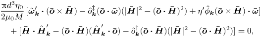 \begin{align} &\frac{{\rm \pi} d^{3} \eta_0}{2 \mu_0 M}\,[\hat{\boldsymbol{\omega}}'_{\boldsymbol{k}} \boldsymbol{\cdot} (\bar{\boldsymbol{o}} \times \bar{\boldsymbol{H}}) - \hat{o}^{\ddagger}_{\boldsymbol{k}} (\bar{\boldsymbol{o}} \boldsymbol{\cdot} \bar{\boldsymbol{\omega}})(|\bar{\boldsymbol{H}}|^{2} - (\bar{\boldsymbol{o}} \boldsymbol{\cdot} \bar{\boldsymbol{H}})^{2}) + \eta^{\prime} \hat{\phi}_{\boldsymbol{k}} (\bar{\boldsymbol{o}} \times \bar{\boldsymbol{H}}) \boldsymbol{\cdot} \bar{\boldsymbol{\omega}}] \nonumber\\ &\quad + [\bar{\boldsymbol{H}} \boldsymbol{\cdot} \hat{\boldsymbol{H}}'_{\boldsymbol{k}} - (\bar{\boldsymbol{o}} \boldsymbol{\cdot} \bar{\boldsymbol{H}})(\hat{\boldsymbol{H}}'_{\boldsymbol{k}} \boldsymbol{\cdot} \bar{\boldsymbol{o}}) - \hat{o}^{{{\dagger}}}_{\boldsymbol{k}} (\bar{\boldsymbol{o}} \boldsymbol{\cdot} \bar{\boldsymbol{H}})(|\bar{\boldsymbol{H}}|^{2} - (\bar{\boldsymbol{o}} \boldsymbol{\cdot} \bar{\boldsymbol{H}})^{2})] = 0, \end{align}
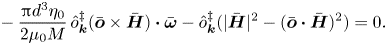 \begin{align} &- \frac{{\rm \pi} d^{3} \eta_0}{2 \mu_0 M}\,\hat{o}^{\ddagger}_{\boldsymbol{k}} (\bar{\boldsymbol{o}} \times \bar{\boldsymbol{H}}) \boldsymbol{\cdot} \bar{\boldsymbol{\omega}} - \hat{o}^{\ddagger}_{\boldsymbol{k}} (|\bar{\boldsymbol{H}}|^{2} - (\bar{\boldsymbol{o}} \boldsymbol{\cdot} \bar{\boldsymbol{H}})^{2}) = 0. \end{align}
These equations are solved to obtain
 \begin{align} \hat{o}^{{{\dagger}}}_{\boldsymbol{k}}& = \frac{{\rm \pi} \eta_0 d^{3} \hat{\boldsymbol{\omega}}'_{\boldsymbol{k}} \boldsymbol{\cdot} (\bar{\boldsymbol{o}} \times \bar{\boldsymbol{H}})}{2 \mu_0 M (\bar{\boldsymbol{o}} \boldsymbol{\cdot} \bar{\boldsymbol{H}})(|\bar{\boldsymbol{H}}|^{2} - (\bar{\boldsymbol{o}} \boldsymbol{\cdot} \bar{\boldsymbol{H}})^{2})} + \frac{\bar{\boldsymbol{H}} \boldsymbol{\cdot} \hat{\boldsymbol{H}}'_{\boldsymbol{k}} - (\bar{\boldsymbol{o}} \boldsymbol{\cdot} \bar{\boldsymbol{H}})(\bar{\boldsymbol{o}} \boldsymbol{\cdot} \hat{\boldsymbol{H}}'_{\boldsymbol{k}})}{(\bar{\boldsymbol{o}} \boldsymbol{\cdot} \bar{\boldsymbol{H}}) (|\bar{\boldsymbol{H}}|^{2} - (\bar{\boldsymbol{o}} \boldsymbol{\cdot} \bar{\boldsymbol{H}})^{2})} \nonumber\\ & \quad + \frac{{\rm \pi} d^{3} \eta_0 \eta^{\prime} \hat{\phi}_{\boldsymbol{k}} (\bar{\boldsymbol{o}} \times \bar{\boldsymbol{H}}) \boldsymbol{\cdot} \bar{\boldsymbol{\omega}}}{2 \mu_0 M (\bar{\boldsymbol{o}} \boldsymbol{\cdot} \bar{\boldsymbol{H}})(|\bar{\boldsymbol{H}}|^{2} - (\bar{\boldsymbol{o}} \boldsymbol{\cdot} \bar{\boldsymbol{H}})^{2})}, \end{align}
 \begin{gather} \hat{o}^{\ddagger}_{\boldsymbol{k}} = 0. \end{gather}
 The magnetophoretic diffusion term in (2.16) is simplified by neglecting the term  $\hat {\boldsymbol{H}}''_{\boldsymbol{k}} \boldsymbol{\cdot } \hat {\boldsymbol{o}}_{\boldsymbol{k}}$ in (2.19), since it is much smaller than
  $\hat {\boldsymbol{H}}'_{\boldsymbol{k}}$:
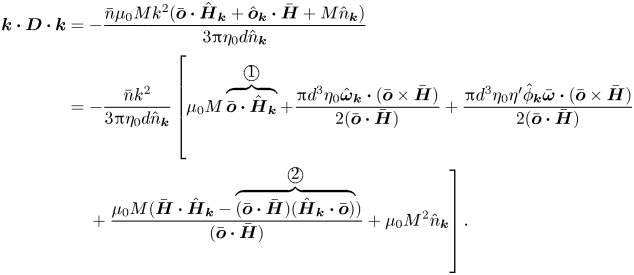 \begin{align} \boldsymbol{k} \boldsymbol{\cdot} \boldsymbol{D} \boldsymbol{\cdot} \boldsymbol{k}& ={-} \frac{\bar{n} \mu_0 M k^{2} (\bar{\boldsymbol{o}} \boldsymbol{\cdot} \hat{\boldsymbol{H}}_{\boldsymbol{k}} + \hat{\boldsymbol{o}}_{\boldsymbol{k}} \boldsymbol{\cdot} \bar{\boldsymbol{H}} + M \hat{n}_{\boldsymbol{k}}) }{3 {\rm \pi}\eta_0 d \hat{n}_{\boldsymbol{k}}} \nonumber\\ & ={-} \frac{\bar{n} k^{2}}{3 {\rm \pi}\eta_0 d \hat{n}_{\boldsymbol{k}}} \left[\vphantom{\left. {}+ \frac{\mu_0 M (\bar{\boldsymbol{H}} \boldsymbol{\cdot} \hat{\boldsymbol{H}}_{\boldsymbol{k}} - \overbrace{(\bar{\boldsymbol{o}} \boldsymbol{\cdot} \bar{\boldsymbol{H}})(\hat{\boldsymbol{H}}_{\boldsymbol{k}} \boldsymbol{\cdot} \bar{\boldsymbol{o}})}^{\unicode{x2461}})}{(\bar{\boldsymbol{o}} \boldsymbol{\cdot} \bar{\boldsymbol{H}})} + \mu_0 M^{2} \hat{n}_{\boldsymbol{k}} \right]} \mu_0 M \overbrace{\bar{\boldsymbol{o}} \boldsymbol{\cdot} \hat{\boldsymbol{H}}_{\boldsymbol{k}}}^{\unicode{x2460}} + \frac{{\rm \pi} d^{3} \eta_0 \hat{\boldsymbol{\omega}}_{\boldsymbol{k}} \boldsymbol{\cdot} (\bar{\boldsymbol{o}} \times \bar{\boldsymbol{H}})}{2 (\bar{\boldsymbol{o}} \boldsymbol{\cdot} \bar{\boldsymbol{H}})} + \frac{{\rm \pi} d^{3} \eta_0 \eta^{\prime} \hat{\phi}_{\boldsymbol{k}} \bar{\boldsymbol{\omega}} \boldsymbol{\cdot} (\bar{\boldsymbol{o}} \times \bar{\boldsymbol{H}})}{2 (\bar{\boldsymbol{o}} \boldsymbol{\cdot} \bar{\boldsymbol{H}})} \right. \nonumber\\ &\quad \left. {}+ \frac{\mu_0 M (\bar{\boldsymbol{H}} \boldsymbol{\cdot} \hat{\boldsymbol{H}}_{\boldsymbol{k}} - \overbrace{(\bar{\boldsymbol{o}} \boldsymbol{\cdot} \bar{\boldsymbol{H}})(\hat{\boldsymbol{H}}_{\boldsymbol{k}} \boldsymbol{\cdot} \bar{\boldsymbol{o}})}^{\unicode{x2461}})}{(\bar{\boldsymbol{o}} \boldsymbol{\cdot} \bar{\boldsymbol{H}})} + \mu_0 M^{2} \hat{n}_{\boldsymbol{k}} \right]. \end{align}
Here, the right-hand sides of (2.29) and (2.33)–(2.34) have been substituted for  $\hat {\boldsymbol{o}}_{\boldsymbol{k}}$ in the second step. In (2.35), the terms
  $\unicode{x2460}$ and
  $\unicode{x2461}$ cancel. The term
  $\unicode{x2460}$ is the contribution due to the interaction between the undisturbed particle magnetic moment and the disturbance to the magnetic field due to particle interactions. This cancels exactly with one of the terms resulting from the disturbance to the particle orientation; the remaining terms are due entirely to the interaction between the undisturbed magnetic field and the disturbance to the particle orientation due to interactions:
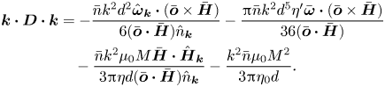 \begin{align} \boldsymbol{k} \boldsymbol{\cdot} \boldsymbol{D} \boldsymbol{\cdot} \boldsymbol{k}& ={-} \frac{\bar{n} k^{2} d^{2} \hat{\boldsymbol{\omega}}_{\boldsymbol{k}} \boldsymbol{\cdot} (\bar{\boldsymbol{o}} \times \bar{\boldsymbol{H}})}{6 (\bar{\boldsymbol{o}} \boldsymbol{\cdot} \bar{\boldsymbol{H}}) \hat{n}_{\boldsymbol{k}}} - \frac{{\rm \pi} \bar{n} k^{2} d^{5} \eta^{\prime} \bar{\boldsymbol{\omega}} \boldsymbol{\cdot} (\bar{\boldsymbol{o}} \times \bar{\boldsymbol{H}})}{36 (\bar{\boldsymbol{o}} \boldsymbol{\cdot} \bar{\boldsymbol{H}})} \nonumber\\ & \quad - \frac{\bar{n} k^{2} \mu_0 M \bar{\boldsymbol{H}} \boldsymbol{\cdot} \hat{\boldsymbol{H}}_{\boldsymbol{k}}}{3 {\rm \pi}\eta d (\bar{\boldsymbol{o}} \boldsymbol{\cdot} \bar{\boldsymbol{H}}) \hat{n}_{\boldsymbol{k}}} - \frac{k^{2} \bar{n} \mu_0 M^{2}}{3 {\rm \pi}\eta_0 d}. \end{align}
Here, the substitution  $\hat {\phi }_{\boldsymbol{k}} = \hat {n}_{\boldsymbol{k}} ({\rm \pi} d^{3}/6)$ has been used to relate the volume fraction and number density in the third term on the right. The first term on the right is due to the disturbance to the orientation vector caused by the hydrodynamic interactions, and the third term results from the disturbance to the orientation vector caused by magnetic interactions. The expressions (2.20a,b) and (2.25) are substituted for the disturbance to the magnetic field and vorticity due to particle interactions, to obtain
 \begin{align} \boldsymbol{k} \boldsymbol{\cdot} \boldsymbol{D} \boldsymbol{\cdot} \boldsymbol{k} & ={-} \frac{{\rm \pi} \bar{n} d^{5} \{ [\boldsymbol{k} \boldsymbol{\cdot} (\bar{\boldsymbol{\omega}} - \bar{\boldsymbol{o}} (\bar{\boldsymbol{o}} \boldsymbol{\cdot} \bar{\boldsymbol{\omega}}))] [\boldsymbol{k} \boldsymbol{\cdot} (\bar{\boldsymbol{o}} \times \bar{\boldsymbol{H}})] - k^{2} [\bar{\boldsymbol{\omega}} - \bar{\boldsymbol{o}} (\bar{\boldsymbol{o}} \boldsymbol{\cdot} \bar{\boldsymbol{\omega}})] \boldsymbol{\cdot} [\bar{\boldsymbol{o}} \times \bar{\boldsymbol{H}}] \}}{24 (\bar{\boldsymbol{o}} \boldsymbol{\cdot} \bar{\boldsymbol{H}})} \nonumber\\ &\quad + \frac{\bar{n} \mu_0 M^{2} (\boldsymbol{k} \boldsymbol{\cdot} \bar{\boldsymbol{o}})(\boldsymbol{k} \boldsymbol{\cdot} \bar{\boldsymbol{H}})}{3 {\rm \pi}\eta_0 d (\bar{\boldsymbol{o}} \boldsymbol{\cdot} \bar{\boldsymbol{H}})} - \frac{{\rm \pi} \bar{n} k^{2} d^{5} \eta^{\prime} \bar{\boldsymbol{\omega}} \boldsymbol{\cdot} (\bar{\boldsymbol{o}} \times \bar{\boldsymbol{H}})}{36 (\bar{\boldsymbol{o}} \boldsymbol{\cdot} \bar{\boldsymbol{H}})} \nonumber\\ & \quad - \frac{k^{2} \bar{n} \mu_0 M^{2}}{3 {\rm \pi}\eta_0 d}. \end{align}
The cross product  $\bar {\boldsymbol{o}} \times \bar {\boldsymbol{H}}$ in (2.37) is expressed in terms of the vorticity using the torque balance equation (2.8) for the base state:
 \begin{align} \boldsymbol{k} \boldsymbol{\cdot} \boldsymbol{D} \boldsymbol{\cdot} \boldsymbol{k}& = \frac{{\rm \pi} \bar{\phi} d^{5} \eta_0 \{ [\boldsymbol{k} \boldsymbol{\cdot} (\bar{\boldsymbol{\omega}} - \bar{\boldsymbol{o}} (\bar{\boldsymbol{o}} \boldsymbol{\cdot} \bar{\boldsymbol{\omega}}))][\boldsymbol{k} \boldsymbol{\cdot} (\bar{\boldsymbol{\omega}} - \bar{\boldsymbol{o}}(\bar{\boldsymbol{o}} \boldsymbol{\cdot} \bar{\boldsymbol{\omega}}))] - k^{2} [|\bar{\boldsymbol{\omega}}|^{2} - (\bar{\boldsymbol{\omega}} \boldsymbol{\cdot} \bar{\boldsymbol{o}})^{2}] \}}{ 8 \mu_0 M (\bar{\boldsymbol{o}} \boldsymbol{\cdot} \bar{\boldsymbol{H}})} \nonumber\\ &\quad + \frac{2 \bar{\phi} \mu_0 M^{2} (\boldsymbol{k} \boldsymbol{\cdot} \bar{\boldsymbol{o}})(\boldsymbol{k} \boldsymbol{\cdot} \bar{\boldsymbol{H}})}{{\rm \pi}^{2} d^{4} \eta_0 (\bar{\boldsymbol{o}} \boldsymbol{\cdot} \bar{\boldsymbol{H}})} + \frac{{\rm \pi} k^{2} d^{5} \bar{\phi} \eta_0 \eta^{\prime} (|\bar{\boldsymbol{\omega}}|^{2} - (\bar{\boldsymbol{\omega}} \boldsymbol{\cdot} \bar{\boldsymbol{o}})^{2})}{12 \mu_0 (\bar{\boldsymbol{o}} \boldsymbol{\cdot} \bar{\boldsymbol{H}})} \nonumber\\ & \quad - \frac{2 k^{2} \bar{\phi} \mu_0 M^{2}}{{\rm \pi}^{2} \eta_0 d^{4}}. \end{align}
Here, the substitution  $\bar {n} = \bar {\phi } ({\rm \pi} d^{3}/6)^{-1}$ has been made, where
  $\bar {\phi }$ is the volume fraction in the base state. The diffusion coefficient
  $\boldsymbol{D}$ is extracted from (2.38). This is written in scaled form as the sum of a ‘hydrodynamic’ contribution due to the vorticity disturbance, a ‘magnetic’ contribution due to the magnetic field disturbance, and an isotropic contribution due to the variation in viscosity and magnetic permeability with particle volume fraction:
 \begin{equation} \boldsymbol{D} = \bar{\phi} d^{2} |\boldsymbol{\omega}| (\boldsymbol{D}^{h} + \boldsymbol{D}^{m} + {D_i^{\prime}} \boldsymbol{I}), \end{equation}
where the scaled diffusivities are
 \begin{gather} \boldsymbol{D}^{h} = \frac{\{ ({{\boldsymbol{e}}_{\bar{\boldsymbol{\omega}}}} - \bar{\boldsymbol{o}} (\bar{\boldsymbol{o}} \boldsymbol{\cdot} {{\boldsymbol{e}}_{\bar{\boldsymbol{\omega}}}})) ({{\boldsymbol{e}}_{\bar{\boldsymbol{\omega}}}} - \bar{\boldsymbol{o}}(\bar{\boldsymbol{o}} \boldsymbol{\cdot} {{\boldsymbol{e}}_{\bar{\boldsymbol{\omega}}}})) - \boldsymbol{I} [1 - ({{\boldsymbol{e}}_{\bar{\boldsymbol{\omega}}}} \boldsymbol{\cdot} \bar{\boldsymbol{o}})^{2}] \}}{ 8\varSigma (\bar{\boldsymbol{o}} \boldsymbol{\cdot} {{\boldsymbol{e}}_{\bar{\boldsymbol{H}}}})}, \end{gather}
 \begin{gather}\boldsymbol{D}^{m} = \frac{\varSigma {M^{{\ast}}}}{\rm \pi} \left( \frac{\bar{\boldsymbol{o}} {{\boldsymbol{e}}_{\bar{\boldsymbol{H}}}} + {{\boldsymbol{e}}_{\bar{\boldsymbol{H}}}} \bar{\boldsymbol{o}}}{\bar{\boldsymbol{o}} \boldsymbol{\cdot} {{\boldsymbol{e}}_{\bar{\boldsymbol{H}}}}} - 2 \boldsymbol{I} \right), \end{gather}
 \begin{gather}{D_i^{\prime}} = \frac{\eta^{\prime} (1 - ({{\boldsymbol{e}}_{\bar{\boldsymbol{\omega}}}} \boldsymbol{\cdot} \bar{\boldsymbol{o}})^{2})}{12 \varSigma (\bar{\boldsymbol{o}} \boldsymbol{\cdot} {{\boldsymbol{e}}_{\bar{\boldsymbol{H}}}})}. \end{gather}
Here,  ${{\boldsymbol {e}}_{\bar {\boldsymbol{\omega }}}}$ and
  ${{\boldsymbol {e}}_{\bar {\boldsymbol{H}}}}$ are the unit vectors along the applied vorticity and magnetic fields, and the substitutions
  $\bar {\boldsymbol{\omega }} = |\bar {\boldsymbol{\omega }}| {{\boldsymbol {e}}_{\bar {\boldsymbol{\omega }}}}$ and
  $\bar {\boldsymbol{H}} = |\bar {\boldsymbol{H}}| {{\boldsymbol {e}}_{\bar {\boldsymbol{H}}}}$ have been used. There are two dimensionless numbers in (2.40)–(2.42), the scaled ratio of the hydrodynamic and magnetic torques
  $\varSigma$, and the scaled magnetic moment
  ${M^{\ast }}$:
 \begin{gather} \varSigma = \frac{\mu_0 M |\bar{\boldsymbol{H}}|}{{\rm \pi} \eta_0 d^{3} |\bar{\boldsymbol{\omega}}|}, \end{gather}
 \begin{gather}{M^{{\ast}}} = \frac{M}{d^{3} |\bar{\boldsymbol{H}}|}. \end{gather}
 In the diffusion tensor (2.39), the contribution  $\boldsymbol{D}^{m}$ due to the magnetic torque is proportional to
  $\bar {\phi } |\bar {\boldsymbol{\omega }}| d^{2} \varSigma \sim \bar {\phi } \mu _0 M |\bar {\boldsymbol{H}}|/ d \eta _0$ and is independent of the vorticity, but it does depend on the viscosity, the particle magnetic moment and the magnetic field. The contribution
  $\boldsymbol{D}^{h}$ due to the hydrodynamic torque is proportional to
  $\bar {\phi } |\bar {\boldsymbol{\omega }}| d^{2} \varSigma ^{-1} \sim \bar {\phi } d^{5} \eta _0 |\bar {\boldsymbol{\omega }}|^{2}/\mu _0 M |\bar {\boldsymbol{H}}|$, and is proportional to the square of the vorticity and inversely proportional to the magnetic field. The isotropic component
  ${D_i} \boldsymbol{I}$ is due to the variation of the viscosity with the particle volume fraction. This is positive, and it has a damping effect on concentration fluctuations.
2.2. Steady solution
The rotating and steady solutions for the orientation vector for an isolated dipolar spheroid in a magnetic field were derived in Kumaran (Reference Kumaran2020a). Here, the results for a spherical particle are summarised briefly. The orientation of the particle depends on the dimensionless parameter  $\varSigma$ in (2.43). The projections of the orientation vector along the directions of the magnetic field and the vorticity are shown as functions of the parameter
  $\varSigma$ in figure 2. The stable solutions are shown by the blue lines, unstable solutions by the red lines, and neutral solutions by the green lines.
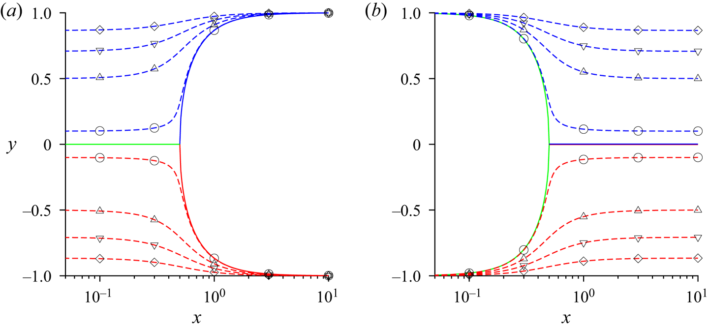
Figure 2. The variation of (a)  $\bar {\boldsymbol{o}} \boldsymbol{\cdot } {{\boldsymbol {e}}_{\bar {\boldsymbol{H}}}}$ and (b)
  $\bar {\boldsymbol{o}} \boldsymbol{\cdot } {{\boldsymbol {e}}_{\bar {\boldsymbol{\omega }}}}$ with
  $\varSigma$ for a particle with a permanent dipole. The solid lines are the results for a parallel magnetic field
  ${{\boldsymbol {e}}_{\bar {\boldsymbol{\omega }}}} \boldsymbol{\cdot } {{\boldsymbol {e}}_{\bar {\boldsymbol{H}}}} = 0$, and the dashed lines are the results for an oblique magnetic field with
  ${{\boldsymbol {e}}_{\bar {\boldsymbol{\omega }}}} \boldsymbol{\cdot } {{\boldsymbol {e}}_{\bar {\boldsymbol{H}}}} = 0.1$ (
 $\circ$),
  $\frac {1}{2}$ (
 $\triangle$),
  $\frac {1}{\sqrt {2}}$ (
 $\nabla$) and
  $\frac {\sqrt {3}}{2}$ (
 $\diamond$). The blue lines are the stable stationary nodes, the red lines are the unstable stationary nodes, and the green lines are the neutral stationary nodes around which there are periodic orbits.
In the limit  $\varSigma \rightarrow \infty$, the orientation vector is parallel to the magnetic field; this corresponds to
  $\bar {\boldsymbol{o}} \boldsymbol{\cdot } {{\boldsymbol {e}}_{\bar {\boldsymbol{H}}}} \rightarrow 1$ for the stable solution. There is also an unstable solution where the orientation vector is anti-parallel to the magnetic field, in which case
  $\bar {\boldsymbol{o}} \boldsymbol{\cdot } {{\boldsymbol {e}}_{\bar {\boldsymbol{H}}}} \rightarrow -1$. As
  $\varSigma$ decreases, there is a gradual decrease in
  $\bar {\boldsymbol{o}} \boldsymbol{\cdot } {{\boldsymbol {e}}_{\bar {\boldsymbol{H}}}}$, while
  $\bar {\boldsymbol{o}} \boldsymbol{\cdot } {{\boldsymbol {e}}_{\bar {\boldsymbol{\omega }}}}$ increases and tends to
  $1$ for the stable solution in this limit. This implies that the particle is aligned along the vorticity direction in the limit
  $\varSigma \rightarrow 0$.
The parallel magnetic field,  ${{\boldsymbol {e}}_{\bar {\boldsymbol{\omega }}}} \boldsymbol{\cdot } {{\boldsymbol {e}}_{\bar {\boldsymbol{H}}}} = 0$, is a special case. In figure 2, it is observed that there is a transition with a slope discontinuity in this case for
  $\varSigma = \frac {1}{2}$. The stable and unstable branches merge and bifurcate into two centre nodes, around which there are periodic closed orbits. There are no steady solutions in this case, and the distribution of orientations in the different orbits depends on the initial distribution. The effect of interactions for a parallel magnetic field is examined in § 2.3 for the parameter regime
  $\varSigma > \frac {1}{2}$, where there is a steady solution. The same study for an oblique magnetic field is presented in § 2.4 for
  $\varSigma > 0$, since there is a steady solution for all values of
  $\varSigma$.
2.3. Parallel magnetic field
Here, we consider the special case where the imposed magnetic field is in the flow plane and perpendicular to the vorticity,  $\bar {\boldsymbol{H}} \boldsymbol{\cdot } \bar {\boldsymbol{\omega }} = 0$. From (2.9),
  $\bar {\boldsymbol{o}} \boldsymbol{\cdot } \bar {\boldsymbol{\omega }} = 0$ for steady solutions, that is, the orientation vector and the vorticity are also orthogonal. The configuration and coordinate system are shown in figure 3(a). A linear shear flow, shown by grey arrows, is applied in the fluid far from the particle. The mean vorticity is in the direction perpendicular to the plane of shear, and the magnetic field vector is in the plane of shear. The orthogonal unit vectors
  ${{\boldsymbol {e}}_{\bar {\boldsymbol{\omega }}}} = \bar {\boldsymbol{\omega }}/|\bar {\boldsymbol{\omega }}|$ and
  ${{\boldsymbol {e}}_{\bar {\boldsymbol{H}}}} = \bar {\boldsymbol{H}} / |\bar {\boldsymbol{H}}|$ are defined along the vorticity and magnetic field directions, and the third orthogonal vector
 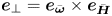 ${{\boldsymbol {e}}_\perp } = {{\boldsymbol {e}}_{\bar {\boldsymbol{\omega }}}} \times {{\boldsymbol {e}}_{\bar {\boldsymbol{H}}}}$ is perpendicular to the
  ${{\boldsymbol {e}}_{\bar {\boldsymbol{\omega }}}}\unicode{x2013}{{\boldsymbol {e}}_{\bar {\boldsymbol{H}}}}$ plane.
Figure 3. The configuration and coordinate system for analysing the effect of interactions for (a) a parallel magnetic field, and (b) an oblique magnetic field. The vorticity vector, shown in blue, is perpendicular to the plane of flow. The applied magnetic field shown in brown and the orientation vector shown in red are in the plane of flow in (a), and at an angle to the plane of flow in (b). The unit vector  ${{\boldsymbol {e}}_\parallel }$ is perpendicular to
  $\bar {\boldsymbol{\omega }}$ in the
  $\bar {\boldsymbol{\omega }}\unicode{x2013}\bar {\boldsymbol{H}}$ plane in (b). The unit vector
  ${{\boldsymbol {e}}_\perp }$ is perpendicular to the
  $\bar {\boldsymbol{\omega }}\unicode{x2013}\bar {\boldsymbol{H}}$ plane.
The solution for the orientation vector for the stable stationary node is
 \begin{gather} \bar{\boldsymbol{o}} \boldsymbol{\cdot} {{\boldsymbol{e}}_{\bar{\boldsymbol{H}}}} = \frac{\sqrt{4 \varSigma^{2} - 1}}{2 \varSigma}, \end{gather}
 \begin{gather}\bar{\boldsymbol{o}} \boldsymbol{\cdot} {{\boldsymbol{e}}_\perp} = \frac{1}{2 \varSigma}. \end{gather}
In (2.39) for the diffusion coefficient, the orientation vector is expressed as  $\bar {\boldsymbol{o}} = \hat {o}_{\boldsymbol{H}} {{\boldsymbol {e}}_{\bar {\boldsymbol{H}}}} + (\bar {\boldsymbol{o}} \boldsymbol{\cdot } {{\boldsymbol {e}}_\perp }) {{\boldsymbol {e}}_\perp }$, and (2.45)–(2.46) are substituted to obtain the diffusion tensor due to hydrodynamic and magnetic interactions:
 \begin{equation} \boldsymbol{D}^{h/m} = \left({{\boldsymbol{e}}_{\bar{\boldsymbol{\omega}}}}\quad {{\boldsymbol{e}}_{\bar{\boldsymbol{H}}}}\quad {{\boldsymbol{e}}_\perp}\right) \left( \begin{array}{ccc} {D_{\bar{\boldsymbol{\omega}} \bar{\boldsymbol{\omega}}}^{h/m}} & 0 & 0 \\ 0 & {D_{\bar{\boldsymbol{H}} \bar{\boldsymbol{H}}}^{h/m}} & {D_{\bar{\boldsymbol{H}} \perp}^{h/m}} \\ 0 & {D_{\bar{\boldsymbol{H}} \perp}^{h/m}} & {D_{{\perp}{\perp}}^{h/m}} \end{array} \right) \left( \begin{array}{c} {{\boldsymbol{e}}_{\bar{\boldsymbol{\omega}}}} \\ {{\boldsymbol{e}}_{\bar{\boldsymbol{H}}}} \\ {{\boldsymbol{e}}_\perp} \end{array} \right), \end{equation}
where
 \begin{gather} {D_{\bar{\boldsymbol{\omega}} \bar{\boldsymbol{\omega}}}^{h}} = 0, \quad {D_{\bar{\boldsymbol{\omega}}\bar{\boldsymbol{\omega}}}^{m}} ={-} \frac{2 \varSigma {M^{{\ast}}}}{\rm \pi}, \end{gather}
 \begin{gather}{D_{\bar{\boldsymbol{H}} \bar{\boldsymbol{H}}}^{h}} ={-} \frac{1}{4 \sqrt{4 \varSigma^{2} - 1}}, \quad {D_{\bar{\boldsymbol{H}} \bar{\boldsymbol{H}}}^{m}} = 0, \end{gather}
 \begin{gather}{D_{\bar{\boldsymbol{H}} \perp}^{h}} = 0, \quad {D_{\bar{\boldsymbol{H}} \perp}^{m}} = \frac{{M^{{\ast}}} \varSigma}{{\rm \pi} \sqrt{4 \varSigma^{2} - 1}}, \end{gather}
 \begin{gather}{D_{{\perp}{\perp}}^{h}} ={-} \frac{1}{4 \sqrt{4 \varSigma^{2} - 1}}, \quad {D_{{\perp}{\perp}}^{m}} ={-} \frac{2 \varSigma {M^{{\ast}}}}{\rm \pi}. \end{gather}
The isotropic contributions to the diffusion tensor due to the concentration dependence of the viscosity and the magnetic permeability are
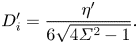 \begin{equation} {D_i^{\prime}} = \frac{\eta^{\prime}}{6 \sqrt{4 \varSigma^{2}-1}}. \end{equation}
 The values of the coefficients in the limit  $\varSigma \gg 1$ and
  $\varSigma - \frac {1}{2} \ll 1$ are listed in table 1. The eigenvalues and eigenvectors of the diffusion matrix are also provided. Since the diffusion matrix is symmetric, the eigenvalues are real, the eigenvectors are orthogonal, and the eigenvectors are the principal directions of amplification (along the directions with negative eigenvalues) or damping (along the directions with positive eigenvalues). If all three principal eigenvalues are negative, then there is amplification of concentration fluctuations in all three directions and the instability is expected to be in the form of particle clusters. If two eigenvalues are negative and one is positive, then there is amplification in two directions and damping in one direction, resulting in rod-like aggregates aligned along the direction with positive eigenvalue. If one eigenvalue is negative and two are positive, then there is amplification along one direction and damping along the other two directions, resulting in the formation of planar aggregates perpendicular to the unstable direction.
Table 1. The asymptotic behaviour of the diffusion coefficients for  $\varSigma, \varSigma _i \gg 1$ and close to the transition from steady to rotating states for a parallel magnetic field for permanent and induced dipoles.
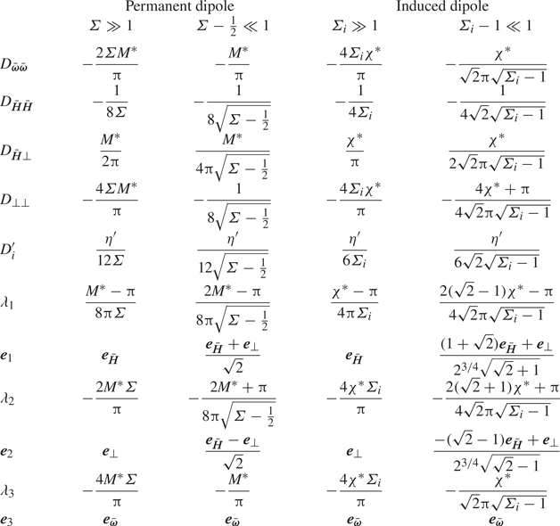
The isotropic part of the diffusion tensor  ${D_i}$ due to the dependence of viscosity on concentration, shown as a function of
  $\varSigma$ in figure 4, is not included in the calculation of the eigenvalues in table 1. When the isotropic part is included, the eigenvectors remain unchanged and the eigenvalues transform as
  $\lambda \rightarrow \lambda + {D_i}$.
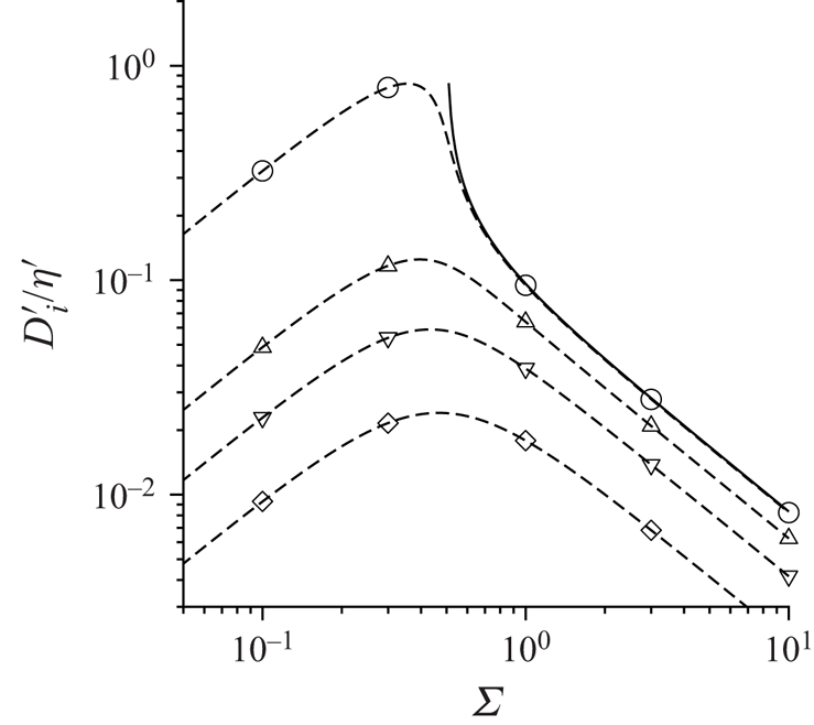
Figure 4. The scaled isotropic part of the diffusion tensor,  ${D_i^{\prime }}/\eta ^{\prime }$ as a function of the parameter
  $\varSigma$ for particles with a permanent dipole. Here,
  ${D_i^{\prime }}$ is given in (2.42). The orientations of the vorticity and magnetic field are
  ${{\boldsymbol {e}}_{\bar {\boldsymbol{\omega }}}} \boldsymbol{\cdot } {{\boldsymbol {e}}_{\bar {\boldsymbol{H}}}} = 0.1$ (
 $\circ$),
  $\frac {1}{2}$ (
 $\triangle$),
  $\frac {1}{\sqrt {2}}$ (
 $\nabla$) and
  $\frac {\sqrt {3}}{2}$ (
 $\diamond$). The solid line is the result for a parallel magnetic field.
Equation (2.47) shows that one of the principal directions is always the vorticity direction, and the diffusion coefficient in this direction is negative, resulting in concentration amplification in this direction for all values of  $\varSigma$. The magnitude of this diffusion coefficient increases proportional to
  $\varSigma {M^{\ast }}$ for
  $\varSigma \gg 1$. This diffusion is due to the modification of the magnetic field by fluctuations in the particle number density, which is the last term in the square brackets on the right in (2.11).
The diffusion in the flow plane is anisotropic, and the diffusion coefficients contain contributions due to hydrodynamic and magnetic interactions. The principal directions for diffusion in the plane, which are the eigenvectors of the  $2 \times 2$ square sub-matrix in (2.47), are presented in table 1 for high magnetic field in the limit
  $\varSigma \gg 1$, and close to the transition between static and rotating states
  $\varSigma - \frac {1}{2} \ll 1$. For
  $\varSigma \gg 1$, the two principal axes are along the
  ${{\boldsymbol {e}}_{\bar {\boldsymbol{H}}}}$ and
  ${{\boldsymbol {e}}_\perp }$ directions. The eigenvalue is negative along the
  ${{\boldsymbol {e}}_\perp }$ direction with magnitude
  $2 \varSigma {M^{\ast }}/{\rm \pi}$, which is the same as that in the
  ${{\boldsymbol {e}}_{\bar {\boldsymbol{\omega }}}}$ direction. The eigenvalue in the
  ${{\boldsymbol {e}}_{\bar {\boldsymbol{H}}}}$ direction is positive for
  ${M^{\ast }} > {\rm \pi}$, and negative otherwise, and the magnitude is proportional to
  $\varSigma ^{-1}$ in this limit. This implies a weak damping of fluctuations for
  ${M^{\ast }} > {\rm \pi}$, and a weak amplification for
  ${M^{\ast }} < {\rm \pi}$. Thus there is anisotropic clustering with a strong amplification of fluctuations in the two directions perpendicular to the magnetic field, and weak damping or amplification along the magnetic field for
  $\varSigma \gg 1$.
For  $\varSigma - \frac {1}{2} \ll 1$, the diffusion coefficient in the vorticity direction tends to a finite value,
  $- ({M^{\ast }} / {\rm \pi})$. The diffusion coefficients in the flow plane diverge proportional to
  $(\varSigma - \frac {1}{2})^{-1/2}$. The eigenvectors in the flow plane are along the directions rotated by angles
  $- {\rm \pi}/4$ and
  $+ {\rm \pi}/4$, respectively, from the magnetic field direction. One of the eigenvalues is always negative, while the other is positive for
  ${M^{\ast }} > {\rm \pi}/2$ and negative otherwise. In both cases, the eigenvalues diverge proportional to
  $(\varSigma - \frac {1}{2})^{-1/2}$. Thus there is strong concentration amplification along one principal direction in the flow plane, and strong damping in the perpendicular direction for
  ${M^{\ast }} > {\rm \pi}/2$, and strong amplification in both principal directions for
  ${M^{\ast }} < {\rm \pi}/2$.
It should be noted that the divergence proportional to  $(4 \varSigma ^{2} - 1)^{-1/2}$ is the result of a mean-field calculation; a more complex renormalisation group calculation is required to include the effect of fluctuations.
2.4. Oblique magnetic field
Analytical solutions for the steady orientation have been derived for a spherical particle in an oblique magnetic field, where the vorticity and magnetic field are not perpendicular. The orthogonal coordinate system shown in figure 3(b) is used, where the unit vector  ${{\boldsymbol {e}}_{\bar {\boldsymbol{\omega }}}}$ is along the vorticity direction,
  ${{\boldsymbol {e}}_\parallel }$ is perpendicular to
  ${{\boldsymbol {e}}_{\bar {\boldsymbol{\omega }}}}$ in the
  ${{\boldsymbol {e}}_{\bar {\boldsymbol{\omega }}}}\unicode{x2013}{{\boldsymbol {e}}_{\bar {\boldsymbol{H}}}}$ plane, and
  ${{\boldsymbol {e}}_\perp }$ is perpendicular to the
  ${{\boldsymbol {e}}_{\bar {\boldsymbol{\omega }}}}\unicode{x2013}{{\boldsymbol {e}}_{\bar {\boldsymbol{H}}}}$ plane. The following notations are used for the dot products:
 \begin{equation} \hat{\omega}_{\boldsymbol{H}} = {{\boldsymbol{e}}_{\bar{\boldsymbol{\omega}}}} \boldsymbol{\cdot} {{\boldsymbol{e}}_{\bar{\boldsymbol{H}}}}, \quad \hat{o}_{\boldsymbol{H}} = \bar{\boldsymbol{o}} \boldsymbol{\cdot} {{\boldsymbol{e}}_{\bar{\boldsymbol{H}}}}. \end{equation}
It should be noted that  $\hat {\omega }_{\boldsymbol{H}}$ is specified, since it depends on the relative orientation of the vorticity and magnetic field, whereas
  $\hat {o}_{\boldsymbol{H}}$ is determined from the solution for the orientation vector. From (2.9), the dot product
  $\bar {\boldsymbol{o}} \boldsymbol{\cdot } {{\boldsymbol {e}}_{\bar {\boldsymbol{\omega }}}}$ is
  $\hat {\omega }_{\boldsymbol{H}}/\hat {o}_{\boldsymbol{H}}$. The unit vectors
  ${{\boldsymbol {e}}_\parallel }$ and
  ${{\boldsymbol {e}}_\perp }$ are
 \begin{gather} {{\boldsymbol{e}}_\parallel} = \frac{{{\boldsymbol{e}}_{\bar{\boldsymbol{H}}}} - \hat{\omega}_{\boldsymbol{H}} {{\boldsymbol{e}}_{\bar{\boldsymbol{\omega}}}}}{\sqrt{1 - \hat{\omega}_{\boldsymbol{H}}^{2}}}, \end{gather}
 \begin{gather}{{\boldsymbol{e}}_\perp} = \frac{{{\boldsymbol{e}}_{\bar{\boldsymbol{\omega}}}} \times {{\boldsymbol{e}}_{\bar{\boldsymbol{H}}}}}{\sqrt{1 - \hat{\omega}_{\boldsymbol{H}}^{2}}}. \end{gather}
The orientation vector for the steady solution is specified by
 \begin{gather} \bar{\boldsymbol{o}} \boldsymbol{\cdot} {{\boldsymbol{e}}_{\bar{\boldsymbol{\omega}}}} = \sqrt{- \frac{4 \varSigma^{2}-1}{2} + \frac{\sqrt{(4 \varSigma^{2} - 1)^{2} + 16 \varSigma^{2} \hat{\omega}_{\boldsymbol{H}}^{2}}}{2}}, \end{gather}
 \begin{gather}\hat{o}_{\boldsymbol{H}} = \frac{1}{2 \varSigma} \sqrt{\frac{4 \varSigma^{2}-1}{2} + \frac{\sqrt{(4 \varSigma^{2} - 1)^{2} + 16 \varSigma^{2} \hat{\omega}_{\boldsymbol{H}}^{2}}}{2}}. \end{gather}
The projection of the orientation vector on the unit vector  ${{\boldsymbol {e}}_\parallel }$ is
 \begin{equation} \bar{\boldsymbol{o}} \boldsymbol{\cdot} {{\boldsymbol{e}}_\parallel} = \frac{\hat{\omega}_{\boldsymbol{H}}(1 - (\bar{\boldsymbol{o}} \boldsymbol{\cdot} {{\boldsymbol{e}}_{\bar{\boldsymbol{\omega}}}})^{2})}{ (\bar{\boldsymbol{o}} \boldsymbol{\cdot} {{\boldsymbol{e}}_{\bar{\boldsymbol{\omega}}}}) \sqrt{1 - \hat{\omega}_{\boldsymbol{H}}^{2}}}. \end{equation}
The dot product  $\bar {\boldsymbol{o}} \boldsymbol{\cdot } {{\boldsymbol {e}}_\perp }$ is determined from the torque balance equation:
 \begin{align} \bar{\boldsymbol{o}} \boldsymbol{\cdot} {{\boldsymbol{e}}_\perp} & = \frac{\bar{\boldsymbol{o}} \boldsymbol{\cdot} ({{\boldsymbol{e}}_{\bar{\boldsymbol{\omega}}}} \times {{\boldsymbol{e}}_{\bar{\boldsymbol{H}}}})}{\sqrt{1 - ({{\boldsymbol{e}}_{\bar{\boldsymbol{\omega}}}} \boldsymbol{\cdot} {{\boldsymbol{e}}_{\bar{\boldsymbol{H}}}})^{2}}} ={-} \frac{{{\boldsymbol{e}}_{\bar{\boldsymbol{\omega}}}} \boldsymbol{\cdot} (\bar{\boldsymbol{o}} \times {{\boldsymbol{e}}_{\bar{\boldsymbol{H}}}})}{\sqrt{1 - ({{\boldsymbol{e}}_{\bar{\boldsymbol{\omega}}}} \boldsymbol{\cdot} {{\boldsymbol{e}}_{\bar{\boldsymbol{H}}}})^{2}}} \nonumber\\ & = \frac{{{\boldsymbol{e}}_{\bar{\boldsymbol{\omega}}}} \boldsymbol{\cdot} (\boldsymbol{I} - \bar{\boldsymbol{o}} \bar{\boldsymbol{o}}) \boldsymbol{\cdot} {{\boldsymbol{e}}_{\bar{\boldsymbol{\omega}}}}}{2 \varSigma \sqrt{1 - ({{\boldsymbol{e}}_{\bar{\boldsymbol{\omega}}}} \boldsymbol{\cdot} {{\boldsymbol{e}}_{\bar{\boldsymbol{H}}}})^{2}}} = \frac{1 - (\bar{\boldsymbol{o}} \boldsymbol{\cdot} {{\boldsymbol{e}}_{\bar{\boldsymbol{\omega}}}})^{2}}{2 \varSigma \sqrt{1 - \hat{\omega}_{\boldsymbol{H}}^{2}}}. \end{align}
The torque balance equation (2.8) and the definition (2.43) of  $\varSigma$ have been used in the third step in the above equation. Equations (2.57)–(2.59) are substituted into (2.39) to obtain (2.47) for the diffusion coefficient, where
  $\boldsymbol{D}^{h}$ and
  $\boldsymbol{D}^{m}$ are symmetric tensors of the form
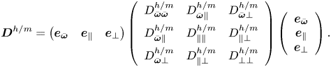 \begin{equation} \boldsymbol{D}^{h/m} = \left({{\boldsymbol{e}}_{\bar{\boldsymbol{\omega}}}} \quad {{\boldsymbol{e}}_\parallel} \quad {{\boldsymbol{e}}_\perp}\right) \left( \begin{array}{ccc} {D_{\bar{\boldsymbol{\omega}} \bar{\boldsymbol{\omega}}}^{h/m}} & {D_{\bar{\boldsymbol{\omega}} \parallel}^{h/m}} & {D_{\bar{\boldsymbol{\omega}} \perp}^{h/m}} \\[5pt] {D_{\bar{\boldsymbol{\omega}} \parallel}^{h/m}} & {D_{{\parallel}{\parallel}}^{h/m}} & {D_{{\parallel}{\perp}}^{h/m}} \\[5pt] {D_{\bar{\boldsymbol{\omega}} \perp}^{h/m}} & {D_{{\parallel}{\perp}}^{h/m}} & {D_{{\perp}{\perp}}^{h/m}} \end{array} \right) \left( \begin{array}{c} {{\boldsymbol{e}}_{\bar{\boldsymbol{\omega}}}} \\ {{\boldsymbol{e}}_\parallel} \\ {{\boldsymbol{e}}_\perp} \end{array} \right). \end{equation}
The solutions for the elements of the tensors  $\boldsymbol{D}^{h}$ and
  $\boldsymbol{D}^{m}$, and the asymptotic expansion of these elements for small and large
  $\varSigma$, are provided in table 2. The elements of
  $\boldsymbol{D}^{h}$ and
  $\boldsymbol{D}^{m}$ do depend on the solution (2.57) for
  $\hat {o}_{\boldsymbol{H}}$, and the asymptotic expansions employ the small and large
  $\varSigma$ approximations for the
  $\hat {o}_{\boldsymbol{H}}$ solution:
 \begin{gather} \hat{o}_{\boldsymbol{H}} = \hat{\omega}_{\boldsymbol{H}} + 2 \varSigma^{2} \hat{\omega}_{\boldsymbol{H}} (1 - \hat{\omega}_{\boldsymbol{H}}^{2}) \quad \mbox{for} \ \varSigma \ll 1, \end{gather}
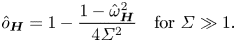 \begin{gather}\hat{o}_{\boldsymbol{H}} = 1 - \frac{1 - \hat{\omega}_{\boldsymbol{H}}^{2}}{4 \varSigma^{2}} \quad \mbox{for} \ \varSigma \gg 1. \end{gather}
It is verified easily that the elements of  $\boldsymbol{D}^{h}$ and
  $\boldsymbol{D}^{m}$ reduce to (2.39) for a parallel magnetic field with
  $\hat {\omega }_{\boldsymbol{H}} = 0$.
Table 2. The asymptotic behaviour of the diffusion coefficients for  $\varSigma \gg 1$ and
  $\varSigma \ll 1$ for an oblique magnetic field for particles with permanent dipoles.
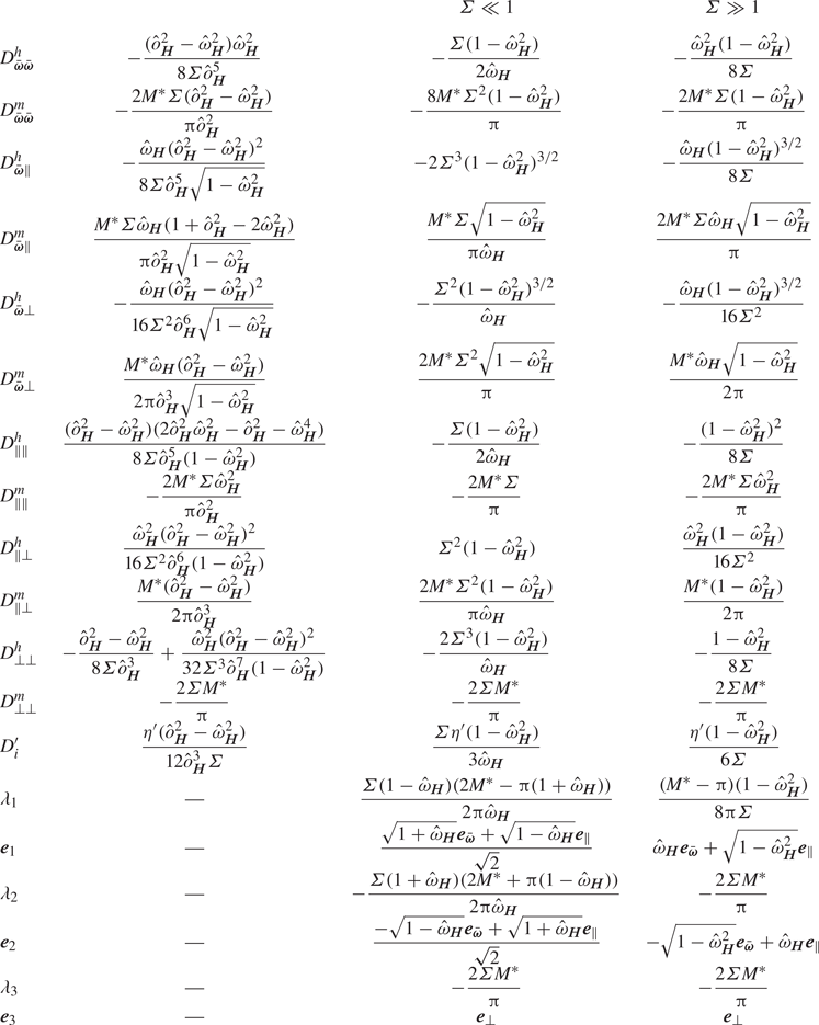
For an oblique magnetic field, all the elements of  $\boldsymbol{D}^{h}$ and
  $\boldsymbol{D}^{m}$ are non-zero. This is in contrast to the diffusion matrix (2.39) for a parallel magnetic field, where there are only five independent non-zero components. For a parallel magnetic field, there is a transition from a static to a rotating state for the orientation vector for a parallel magnetic field at
  $\varSigma = \frac {1}{2}$. In contrast, there is no transition for an oblique magnetic field. Therefore, the diffusion coefficients for a parallel magnetic field are defined only in the range
  $\frac {1}{2} < \varSigma < \infty$, whereas those for an oblique magnetic field are defined for
  $0 < \varSigma < \infty$ in figure 5.
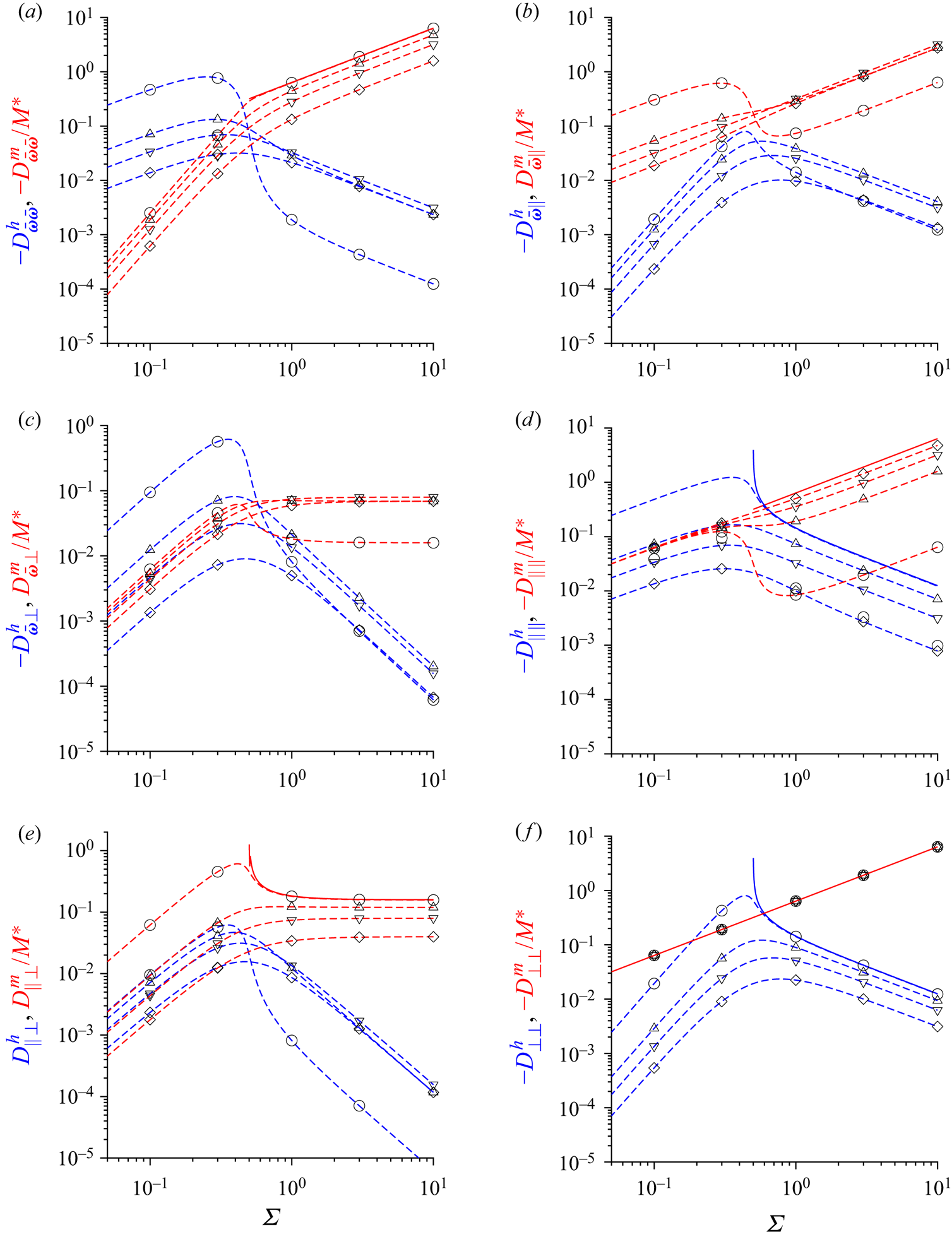
Figure 5. The components of the diffusion tensor: (a)  $- {D_{\bar {\boldsymbol{\omega }} \bar {\boldsymbol{\omega }}}^{h}}$ and
  $- {D_{\bar {\boldsymbol{\omega }}\bar {\boldsymbol{\omega }}}^{m}}/{M^{\ast }}$, (b)
  $- {D_{\bar {\boldsymbol{\omega }} \parallel }^{h}}$ and
  ${D_{\bar {\boldsymbol{\omega }} \parallel }^{m}}/{M^{\ast }}$, (c)
  $- {D_{\bar {\boldsymbol{\omega }} \perp }^{h}}$ and
  ${D_{\bar {\boldsymbol{\omega }} \perp }^{m}}/{M^{\ast }}$, (d)
  $- {D_{\parallel \parallel }^{h}}$ and
  $- {D_{\parallel \parallel }^{m}}/{M^{\ast }}$, (e)
  ${D_{\parallel \perp }^{h}}$ and
  ${D_{\parallel \perp }^{m}}/{M^{\ast }}$, and (f)
  $- {D_{\perp \perp }^{h}}$ and
  $- {D_{\perp \perp }^{m}}/{M^{\ast }}$, due to hydrodynamic interactions (blue lines) and magnetic interactions (red lines) as functions of the parameter
  $\varSigma$ for particles with a permanent dipole. The orientations of the vorticity and magnetic field are
  ${{\boldsymbol {e}}_{\bar {\boldsymbol{\omega }}}} \boldsymbol{\cdot } {{\boldsymbol {e}}_{\bar {\boldsymbol{H}}}} = 0.1$ (
 $\circ$),
  $\frac {1}{2}$ (
 $\triangle$),
  $\frac {1}{\sqrt {2}}$ (
 $\nabla$) and
  $\frac {\sqrt {3}}{2}$ (
 $\diamond$). The solid red and blue lines are the non-zero results for a parallel magnetic field.
Table 2 shows that all components of the hydrodynamic contribution to the diffusion tensor  $\boldsymbol{D}^{h}$ are negative, with the exception of the component
  ${D_{\parallel \perp }^{h}}$. In contrast, all components of the magnetic contribution to the diffusion tensor
  $\boldsymbol{D}^{m}$ are positive. This implies that the magnetic interactions tend to dampen concentration fluctuations and stabilise the uniform state, whereas hydrodynamic interactions tend to destabilise the concentration fluctuations. The diffusion in the direction perpendicular to the vorticity and magnetic field is due entirely to hydrodynamic interactions, and the diffusion coefficient
  ${D_{\perp \perp }}$ is negative. Therefore, concentration fluctuations are amplified in the direction perpendicular to the vorticity and magnetic field. In other directions, the stability is determined by a balance between the contributions due to hydrodynamic and magnetic interactions.
The components of  $\boldsymbol{D}$ are shown as functions of
  $\varSigma$ for different values of
  $\hat {\omega }_{\boldsymbol{H}}$ in figures 4 and 5. Also shown by solid lines in figures 5(a), 5(d), 5(e) and 5(f) are the results for a parallel magnetic field. The components of the diffusion tensor for a parallel magnetic field do not extend to
  $\varSigma < \frac {1}{2}$, due to the transition to a rotating state; the divergence in the diffusion coefficients
  ${D_{\bar {\boldsymbol{H}} \bar {\boldsymbol{H}}}^{h}}$,
  ${D_{\bar {\boldsymbol{H}} \perp }^{m}}$ and
  ${D_{\perp \perp }^{h}}$ predicted by (2.49a,b)–(2.51a,b) is apparent in figure 5. The results for
  $\hat {\omega }_{\boldsymbol{H}} = 0.1$ are in close agreement with those for a parallel magnetic field for
  $\varSigma \gtrsim \frac {1}{2}$, but the divergence in the coefficients
  ${D_{\bar {\boldsymbol{H}} \bar {\boldsymbol{H}}}^{h}}$,
  ${D_{\bar {\boldsymbol{H}} \perp }^{m}}$ and
  ${D_{\perp \perp }^{h}}$ is cut off, and the diffusion coefficients are finite,
  $\varSigma < \frac {1}{2}$.
The coefficients  ${D_{\bar {\boldsymbol{\omega }} \bar {\boldsymbol{\omega }}}^{h}}, {D_{\bar {\boldsymbol{\omega }} \parallel }^{h}}, {D_{\bar {\boldsymbol{\omega }} \parallel }^{m}}, {D_{\bar {\boldsymbol{\omega }} \perp }^{h}}, {D_{\bar {\boldsymbol{\omega }} \perp }^{m}}, {D_{\parallel \parallel }^{m}}, {D_{\parallel \perp }^{h}}$ are all zero for a parallel magnetic field with
  $\hat {\omega }_{\boldsymbol{H}} = 0$. Figure 5 shows that these coefficients do decrease as
  $\hat {\omega }_{\boldsymbol{H}}$ decreases for
  $\varSigma > \frac {1}{2}$, in accordance with the
  $\varSigma \gg 1$ expressions in table 2. For
  $\varSigma < \frac {1}{2}$, these do not decrease as
  $\hat {\omega }_{\boldsymbol{H}}$ decreases. The latter regime is not accessible for a parallel magnetic field, since there is no steady orientation. Therefore, the diffusion due to interactions for a nearly parallel magnetic field is qualitatively different from that in a parallel magnetic field, due to the transition to rotating states in the latter.
The magnetic contributions to the diffusion tensor are larger than the hydrodynamic contributions for  $\varSigma \gg 1$. For
  $\varSigma \gg 1$, the largest contributions to the diffusion tensor are
  ${D_{\bar {\boldsymbol{\omega }}\bar {\boldsymbol{\omega }}}^{m}}$,
  ${D_{\bar {\boldsymbol{\omega }} \parallel }^{m}}$,
  ${D_{\parallel \parallel }^{m}}$ and
  ${D_{\perp \perp }^{m}}$, which diverge proportional to
  $\varSigma$. The coefficient
  ${D_{\perp \perp }^{m}} = - (2 {M^{\ast }} \varSigma /{\rm \pi} )$ is negative for all
  $\varSigma$, indicating that concentration fluctuations are amplified in the
  ${{\boldsymbol {e}}_\perp }$ direction. The diffusion in the
  ${{\boldsymbol {e}}_{\bar {\boldsymbol{\omega }}}}\unicode{x2013}{{\boldsymbol {e}}_\parallel }$ plane is along two principal directions. The eigenvalue
  $- (2 {M^{\ast }} \varSigma /{\rm \pi} )$ along
  $\boldsymbol{e}_2$ in table 2 also increases proportional to
  $\varSigma$ for
  $\varSigma \gg 1$, indicating strong amplification of concentration fluctuations in this direction. The eigenvalue along the
  $\boldsymbol{e}_1$ direction decreases proportional to
  $\varSigma ^{-1}$ for
  $\varSigma \gg 1$, and the concentration fluctuations are dampened/amplified for
  ${M^{\ast }} \gtrless {\rm \pi}$. Thus the behaviour of concentration fluctuations for
  $\varSigma \gg 1$ is very similar to that for a parallel magnetic field, with strong concentration amplifications in two directions
  ${{\boldsymbol {e}}_\perp }$ and
  $\boldsymbol{e}_2$, and weak amplification/damping in the third perpendicular direction.
In the limit  $\varSigma \ll 1$, the diffusion coefficient along the
  ${{\boldsymbol {e}}_\perp }$ direction perpendicular to the vorticity and magnetic field is
  ${D_{\perp \perp }^{m}} = - (2 {M^{\ast }} \varSigma /{\rm \pi} )$. The
  $O(\varSigma )$ contributions to the diffusion tensor are
  ${D_{\bar {\boldsymbol{\omega }} \bar {\boldsymbol{\omega }}}^{h}}$,
  ${D_{\bar {\boldsymbol{\omega }}\bar {\boldsymbol{\omega }}}^{m}}$,
  ${D_{\parallel \parallel }^{h}}$,
  ${D_{\bar {\boldsymbol{\omega }} \parallel }^{m}}$ and
  ${D_{\perp \perp }^{m}}$. For diffusion in the
  ${{\boldsymbol {e}}_{\bar {\boldsymbol{\omega }}}}\unicode{x2013}{{\boldsymbol {e}}_\parallel }$ plane, concentration fluctuations are unstable along the
  $\boldsymbol{e}_2$ direction where the eigenvalue
  $\lambda _2$ is negative, while they are stable in the perpendicular direction
  $\boldsymbol{e}_1$ for
  $2 {M^{\ast }} > {\rm \pi}(1 + \hat {\omega }_{\boldsymbol{H}})$ and unstable otherwise.
3. Induced dipole
3.1. Diffusion due to interactions
For an induced dipole, the particle magnetic moment is modelled as
 \begin{equation} \boldsymbol{M} = \chi \boldsymbol{o} [\boldsymbol{o} \boldsymbol{\cdot} (\boldsymbol{H} + n \boldsymbol{M})], \end{equation}
that is, the magnetic moment is proportional to the component of the magnetic field along the particle orientation. Here,  $\chi$ is the magnetic susceptibility of the particle. Substituting
  $\boldsymbol{M} = M \boldsymbol{o}$ in (3.1), the magnitude of the particle magnetic moment is
 \begin{equation} M = \frac{\chi \boldsymbol{o} \boldsymbol{\cdot} \boldsymbol{H}}{1 - \chi n}. \end{equation}
The torque balance equation in the absence of interactions in the direction perpendicular to the orientation vector, analogous to (2.8), is
 \begin{equation} \frac{1}{2} {\rm \pi}\eta d^{3} (\boldsymbol{I} - \boldsymbol{o} \boldsymbol{o}) \boldsymbol{\cdot} \boldsymbol{\omega} + \frac{\mu_0 \chi (\boldsymbol{o} \boldsymbol{\cdot} \boldsymbol{H}) (\boldsymbol{o} \times \boldsymbol{H})}{ 1 - \chi n} = 0. \end{equation}
The substitution (3.2) is made in (2.1) to obtain the expression for the force,
 \begin{align} \boldsymbol{F} & = \boldsymbol{\nabla} \left[\frac{\chi (\boldsymbol{o} \boldsymbol{\cdot} \boldsymbol{H})}{1 - \chi n}\,\boldsymbol{o} \boldsymbol{\cdot} \left(\boldsymbol{H} + \frac{\chi n \boldsymbol{o} (\boldsymbol{o} \boldsymbol{\cdot} \boldsymbol{H})}{1 - \chi n} \right) \right] \nonumber\\ & = \boldsymbol{\nabla} \left[ \frac{\chi (\boldsymbol{o} \boldsymbol{\cdot} \boldsymbol{H})^{2}}{(1 - \chi n)^{2}} \right]. \end{align}
When this expression is linearised in the perturbations and transformed into Fourier space, the equivalent of (2.11) for the interaction force is
 \begin{equation} \hat{\boldsymbol{F}}_{\boldsymbol{k}} ={-} 2 {{\rm{i}}} \boldsymbol{k} \mu_0 \chi (\bar{\boldsymbol{o}} \boldsymbol{\cdot} \bar{\boldsymbol{H}}) \left[\frac{ \bar{\boldsymbol{o}} \boldsymbol{\cdot} \hat{\boldsymbol{H}}_{\boldsymbol{k}} + \bar{\boldsymbol{H}} \boldsymbol{\cdot} \hat{\boldsymbol{o}}_{\boldsymbol{k}}}{(1 - \chi \bar{n})^{2}} + \frac{\chi \hat{n}_{\boldsymbol{k}} (\bar{\boldsymbol{o}} \boldsymbol{\cdot} \bar{\boldsymbol{H}})}{(1 - \chi \bar{n})^{3}} \right]. \end{equation}
Since we are considering the limit where the disturbance is small compared to the applied magnetic field, the approximation  $\bar {n} \chi \ll 1$ is made in (3.5). With this approximation, the equivalent of (2.16) for the particle concentration field is
 \begin{equation} \frac{\partial \hat{n}_{\boldsymbol{k}}}{\partial t} + {{\rm{i}}} \boldsymbol{k} \boldsymbol{\cdot} (\bar{\boldsymbol{v}} \hat{n}_{\boldsymbol{k}}) + D_B k^{2} \hat{n}_{\boldsymbol{k}} - \left( \frac{2 k^{2} \bar{n} \mu_0 \chi (\bar{\boldsymbol{o}} \boldsymbol{\cdot} \bar{\boldsymbol{H}}) (\bar{\boldsymbol{o}} \boldsymbol{\cdot} \hat{\boldsymbol{H}}_{\boldsymbol{k}} + \bar{\boldsymbol{H}} \boldsymbol{\cdot} \hat{\boldsymbol{o}}_{\boldsymbol{k}}+\chi \hat{n}_{\boldsymbol{k}} (\bar{\boldsymbol{o}} \boldsymbol{\cdot} \bar{\boldsymbol{H}}))}{3 {\rm \pi}\eta_0 d} \right) = 0. \end{equation}
Comparing (3.6) with (2.17), the magnetophoretic diffusion term in the particle number density equation is
 \begin{equation} \boldsymbol{k} \boldsymbol{\cdot} \boldsymbol{D} \boldsymbol{\cdot} \boldsymbol{k} ={-} \frac{2 k^{2} \bar{n} \mu_0 \chi (\bar{\boldsymbol{o}} \boldsymbol{\cdot} \bar{\boldsymbol{H}}) (\bar{\boldsymbol{o}} \boldsymbol{\cdot} \hat{\boldsymbol{H}}_{\boldsymbol{k}} + \hat{\boldsymbol{o}}_{\boldsymbol{k}} \boldsymbol{\cdot} \bar{\boldsymbol{H}} + \chi \hat{n}_{\boldsymbol{k}} \bar{\boldsymbol{o}} \boldsymbol{\cdot} \bar{\boldsymbol{H}})}{3 {\rm \pi}\eta_0 d \hat{n}_{\boldsymbol{k}}}. \end{equation}
The equivalent of (2.19) for the disturbance to the magnetic field due to interactions is
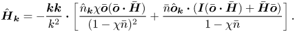 \begin{equation} \hat{\boldsymbol{H}}_{\boldsymbol{k}} ={-} \frac{\boldsymbol{k} \boldsymbol{k}}{k^{2}} \boldsymbol{\cdot} \left[ \frac{\hat{n}_{\boldsymbol{k}} \chi \bar{\boldsymbol{o}} (\bar{\boldsymbol{o}} \boldsymbol{\cdot} \bar{\boldsymbol{H}})}{ (1 - \chi \bar{n})^{2}} + \frac{\bar{n} \hat{\boldsymbol{o}}_{\boldsymbol{k}} \boldsymbol{\cdot} (\boldsymbol{I} (\bar{\boldsymbol{o}} \boldsymbol{\cdot} \bar{\boldsymbol{H}}) + \bar{\boldsymbol{H}} \bar{\boldsymbol{o}})}{1 - \chi \bar{n}} \right]. \end{equation}
The second term in the square brackets on the right, proportional to  $\hat {\boldsymbol{o}}_{\boldsymbol{k}}$, equivalent to the term proportional to
  $\hat {\boldsymbol{H}}''$ in (2.19), is neglected. The reason for this is discussed in the paragraph following (2.28). In the denominator of the first term in the square brackets on the right of (3.8),
  $\chi \bar {n}$ is neglected in comparison to
  $1$, because the disturbance to the magnetic field is small compared to the applied magnetic field. The disturbance to the vorticity field is given in (2.24). In this expression, the term proportional to
  $\bar {n} d^{3}$ on the left-hand side is neglected because the volume fraction is small, and the term proportional to
  $\hat {\boldsymbol{\omega }}''$ on the right-hand side is neglected for the reason discussed in the paragraph after (2.28). With these approximations, the torque balance equation, equivalent to (2.28), is
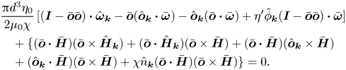 \begin{align} &\frac{{\rm \pi} d^{3} \eta_0}{2 \mu_0 \chi}\,[(\boldsymbol{I} - \bar{\boldsymbol{o}} \bar{\boldsymbol{o}}) \boldsymbol{\cdot} \hat{\boldsymbol{\omega}}_{\boldsymbol{k}} - \bar{\boldsymbol{o}} (\hat{\boldsymbol{o}}_{\boldsymbol{k}} \boldsymbol{\cdot} \bar{\boldsymbol{\omega}}) - \hat{\boldsymbol{o}}_{\boldsymbol{k}} (\bar{\boldsymbol{o}} \boldsymbol{\cdot} \bar{\boldsymbol{\omega}}) + \eta^{\prime} \hat{\phi}_{\boldsymbol{k}} (\boldsymbol{I} - \bar{\boldsymbol{o}} \bar{\boldsymbol{o}}) \boldsymbol{\cdot} \bar{\boldsymbol{\omega}}] \nonumber\\ &\quad + \{(\bar{\boldsymbol{o}} \boldsymbol{\cdot} \bar{\boldsymbol{H}})(\bar{\boldsymbol{o}} \times \hat{\boldsymbol{H}}_{\boldsymbol{k}}) + (\bar{\boldsymbol{o}} \boldsymbol{\cdot} \hat{\boldsymbol{H}}_{\boldsymbol{k}}) (\bar{\boldsymbol{o}} \times \bar{\boldsymbol{H}}) + (\bar{\boldsymbol{o}} \boldsymbol{\cdot} \bar{\boldsymbol{H}}) (\hat{\boldsymbol{o}}_{\boldsymbol{k}} \times \bar{\boldsymbol{H}}) \nonumber\\ &\quad + (\hat{\boldsymbol{o}}_{\boldsymbol{k}} \boldsymbol{\cdot} \bar{\boldsymbol{H}}) (\bar{\boldsymbol{o}} \times \bar{\boldsymbol{H}}) + \chi \hat{n}_{\boldsymbol{k}} (\bar{\boldsymbol{o}} \boldsymbol{\cdot} \bar{\boldsymbol{H}})(\bar{\boldsymbol{o}} \times \bar{\boldsymbol{H}}) \} = 0. \end{align}
The expression (2.29), is substituted into (3.9) to obtain
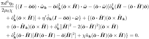 \begin{align} &\frac{{\rm \pi} d^{3} \eta_0}{2 \mu_0 \chi}\,\{(\boldsymbol{I} - \bar{\boldsymbol{o}} \bar{\boldsymbol{o}}) \boldsymbol{\cdot} \hat{\boldsymbol{\omega}}_{\boldsymbol{k}} - \bar{\boldsymbol{o}} \hat{o}^{\ddagger}_{\boldsymbol{k}} (\bar{\boldsymbol{o}} \times \bar{\boldsymbol{H}}) \boldsymbol{\cdot} \bar{\boldsymbol{\omega}} - (\bar{\boldsymbol{o}} \boldsymbol{\cdot} \bar{\boldsymbol{\omega}}) [\hat{o}^{{{\dagger}}}_{\boldsymbol{k}} (\bar{\boldsymbol{H}} - (\bar{\boldsymbol{o}} \boldsymbol{\cdot} \bar{\boldsymbol{H}}) \bar{\boldsymbol{o}}) \nonumber\\ &\quad + \hat{o}^{\ddagger}_{\boldsymbol{k}} (\bar{\boldsymbol{o}} \times \bar{\boldsymbol{H}})] + \eta^{\prime} \hat{\phi}_{\boldsymbol{k}} (\boldsymbol{I} - \bar{\boldsymbol{o}} \bar{\boldsymbol{o}}) \boldsymbol{\cdot} \bar{\boldsymbol{\omega}} \} + \{(\bar{\boldsymbol{o}} \boldsymbol{\cdot} \bar{\boldsymbol{H}})(\bar{\boldsymbol{o}} \times \hat{\boldsymbol{H}}_{\boldsymbol{k}}) \nonumber\\ &\quad + (\bar{\boldsymbol{o}} \boldsymbol{\cdot} \hat{\boldsymbol{H}}_{\boldsymbol{k}}) (\bar{\boldsymbol{o}} \times \bar{\boldsymbol{H}}) + \hat{o}^{{{\dagger}}}_{\boldsymbol{k}} [|\bar{\boldsymbol{H}}|^{2} - 2 (\bar{\boldsymbol{o}} \boldsymbol{\cdot} \bar{\boldsymbol{H}})^{2}] (\bar{\boldsymbol{o}} \times \bar{\boldsymbol{H}}) \nonumber\\ &\quad + \hat{o}^{\ddagger}_{\boldsymbol{k}} (\bar{\boldsymbol{o}} \boldsymbol{\cdot} \bar{\boldsymbol{H}}) [\bar{\boldsymbol{H}} (\bar{\boldsymbol{o}} \boldsymbol{\cdot} \bar{\boldsymbol{H}}) - \bar{\boldsymbol{o}} |\bar{\boldsymbol{H}}|^{2}] + \chi \hat{n}_{\boldsymbol{k}} (\bar{\boldsymbol{o}} \boldsymbol{\cdot} \bar{\boldsymbol{H}})(\bar{\boldsymbol{o}} \times \bar{\boldsymbol{H}}) \} = 0. \end{align}
The functions  $\hat {o}^{{{\dagger}} }_{\boldsymbol{k}}$ and
  $\hat {o}^{\ddagger }_{\boldsymbol{k}}$ are determined by taking the dot product of (3.10) with
  $\bar {\boldsymbol{o}} \times \bar {\boldsymbol{H}}$ and
  $\bar {\boldsymbol{o}}$, respectively:
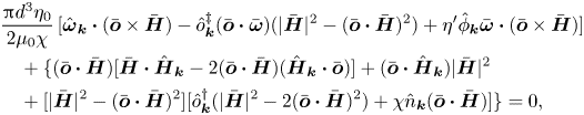 \begin{align} &\frac{{\rm \pi} d^{3} \eta_0}{2 \mu_0 \chi}\,[\hat{\boldsymbol{\omega}}_{\boldsymbol{k}} \boldsymbol{\cdot} (\bar{\boldsymbol{o}} \times \bar{\boldsymbol{H}}) - \hat{o}^{\ddagger}_{\boldsymbol{k}} (\bar{\boldsymbol{o}} \boldsymbol{\cdot} \bar{\boldsymbol{\omega}})(|\bar{\boldsymbol{H}}|^{2} - (\bar{\boldsymbol{o}} \boldsymbol{\cdot} \bar{\boldsymbol{H}})^{2}) + \eta^{\prime} \hat{\phi}_{\boldsymbol{k}} \bar{\boldsymbol{\omega}} \boldsymbol{\cdot} (\bar{\boldsymbol{o}} \times \bar{\boldsymbol{H}})] \nonumber\\ &\quad + \{(\bar{\boldsymbol{o}} \boldsymbol{\cdot} \bar{\boldsymbol{H}})[\bar{\boldsymbol{H}} \boldsymbol{\cdot} \hat{\boldsymbol{H}}_{\boldsymbol{k}} - 2 (\bar{\boldsymbol{o}} \boldsymbol{\cdot} \bar{\boldsymbol{H}})(\hat{\boldsymbol{H}}_{\boldsymbol{k}} \boldsymbol{\cdot} \bar{\boldsymbol{o}})] + (\bar{\boldsymbol{o}} \boldsymbol{\cdot} \hat{\boldsymbol{H}}_{\boldsymbol{k}}) |\bar{\boldsymbol{H}}|^{2} \nonumber\\ &\quad + [|\bar{\boldsymbol{H}}|^{2} - (\bar{\boldsymbol{o}} \boldsymbol{\cdot} \bar{\boldsymbol{H}})^{2}][\hat{o}^{{{\dagger}}}_{\boldsymbol{k}} (|\bar{\boldsymbol{H}}|^{2} - 2 (\bar{\boldsymbol{o}} \boldsymbol{\cdot} \bar{\boldsymbol{H}})^{2}) + \chi \hat{n}_{\boldsymbol{k}} (\bar{\boldsymbol{o}} \boldsymbol{\cdot} \bar{\boldsymbol{H}})] \} = 0, \end{align}
 \begin{align} &- \frac{{\rm \pi} d^{3} \eta_0}{2 \mu_0 \chi}\,[\hat{o}^{\ddagger}_{\boldsymbol{k}} (\bar{\boldsymbol{o}} \times \bar{\boldsymbol{H}}) \boldsymbol{\cdot} \bar{\boldsymbol{\omega}}] - \{ \hat{o}^{\ddagger}_{\boldsymbol{k}} (\bar{\boldsymbol{o}} \boldsymbol{\cdot} \bar{\boldsymbol{H}}) [|\bar{\boldsymbol{H}}|^{2} - (\bar{\boldsymbol{o}} \boldsymbol{\cdot} \bar{\boldsymbol{H}})^{2}] \} = 0. \end{align}
These are solved to obtain
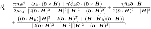 \begin{align} \hat{o}^{{{\dagger}}}_{\boldsymbol{k}} & = \frac{{\rm \pi} \eta_0 d^{3}}{2 \mu_0 \chi}\,\frac{\hat{\boldsymbol{\omega}}_{\boldsymbol{k}} \boldsymbol{\cdot} (\bar{\boldsymbol{o}} \times \bar{\boldsymbol{H}}) + \eta^{\prime} \hat{\phi}_{\boldsymbol{k}} \bar{\boldsymbol{\omega}} \boldsymbol{\cdot} (\bar{\boldsymbol{o}} \times \bar{\boldsymbol{H}})}{[2 (\bar{\boldsymbol{o}} \boldsymbol{\cdot} \bar{\boldsymbol{H}})^{2} - |\bar{\boldsymbol{H}}|^{2}] [|\bar{\boldsymbol{H}}|^{2} - (\bar{\boldsymbol{o}} \boldsymbol{\cdot} \bar{\boldsymbol{H}})^{2}]} + \frac{\chi \hat{n}_{\boldsymbol{k}} \bar{\boldsymbol{o}} \boldsymbol{\cdot} \bar{\boldsymbol{H}}}{2 (\bar{\boldsymbol{o}} \boldsymbol{\cdot} \bar{\boldsymbol{H}})^{2} - |\bar{\boldsymbol{H}}|^{2}} \nonumber\\ & \quad + \frac{\{(\bar{\boldsymbol{o}} \boldsymbol{\cdot} \hat{\boldsymbol{H}}_{\boldsymbol{k}})[|\bar{\boldsymbol{H}}|^{2} - 2 (\bar{\boldsymbol{o}} \boldsymbol{\cdot} \bar{\boldsymbol{H}})^{2}] + (\bar{\boldsymbol{H}} \boldsymbol{\cdot} \hat{\boldsymbol{H}}_{\boldsymbol{k}})(\bar{\boldsymbol{o}} \boldsymbol{\cdot} \bar{\boldsymbol{H}})\}}{[2 (\bar{\boldsymbol{o}} \boldsymbol{\cdot} \bar{\boldsymbol{H}})^{2} - |\bar{\boldsymbol{H}}|^{2}] [|\bar{\boldsymbol{H}}|^{2} - (\bar{\boldsymbol{o}} \boldsymbol{\cdot} \bar{\boldsymbol{H}})^{2}]}, \end{align}
 \begin{gather} \hat{o}^{\ddagger}_{\boldsymbol{k}} = 0. \end{gather}
The expression for the magnetophoretic diffusion in (3.7) is
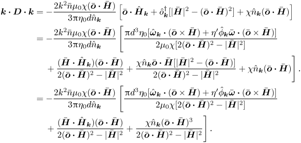 \begin{align} \boldsymbol{k} \boldsymbol{\cdot} \boldsymbol{D} \boldsymbol{\cdot} \boldsymbol{k} & ={-} \frac{2 k^{2} \bar{n} \mu_0 \chi (\bar{\boldsymbol{o}} \boldsymbol{\cdot} \bar{\boldsymbol{H}})}{3 {\rm \pi}\eta_0 d\hat{n}_{\boldsymbol{k}}} \left[ \bar{\boldsymbol{o}} \boldsymbol{\cdot} \hat{\boldsymbol{H}}_{\boldsymbol{k}} + \hat{o}^{{{\dagger}}}_{\boldsymbol{k}} [|\bar{\boldsymbol{H}}|^{2} - (\bar{\boldsymbol{o}} \boldsymbol{\cdot} \bar{\boldsymbol{H}})^{2}] + \chi \hat{n}_{\boldsymbol{k}} (\bar{\boldsymbol{o}} \boldsymbol{\cdot} \bar{\boldsymbol{H}}) \right] \nonumber\\ & ={-} \frac{2 k^{2} \bar{n} \mu_0 \chi (\bar{\boldsymbol{o}} \boldsymbol{\cdot} \bar{\boldsymbol{H}})}{3 {\rm \pi}\eta_0 d \hat{n}_{\boldsymbol{k}}} \left[ \frac{{\rm \pi} d^{3} \eta_0 [\hat{\boldsymbol{\omega}}_{\boldsymbol{k}} \boldsymbol{\cdot} (\bar{\boldsymbol{o}} \times \bar{\boldsymbol{H}}) + \eta^{\prime} \hat{\phi}_{\boldsymbol{k}} \bar{\boldsymbol{\omega}} \boldsymbol{\cdot} (\bar{\boldsymbol{o}} \times \bar{\boldsymbol{H}})]}{2 \mu_0 \chi [2 (\bar{\boldsymbol{o}} \boldsymbol{\cdot} \bar{\boldsymbol{H}})^{2} - |\bar{\boldsymbol{H}}|^{2}]} \right. \nonumber\\ &\quad \left. {}+ \frac{(\bar{\boldsymbol{H}} \boldsymbol{\cdot} \hat{\boldsymbol{H}}_{\boldsymbol{k}}) (\bar{\boldsymbol{o}} \boldsymbol{\cdot} \bar{\boldsymbol{H}})}{2 (\bar{\boldsymbol{o}} \boldsymbol{\cdot} \bar{\boldsymbol{H}})^{2} - |\bar{\boldsymbol{H}}|^{2}} + \frac{\chi \hat{n}_{\boldsymbol{k}} \bar{\boldsymbol{o}} \boldsymbol{\cdot} \bar{\boldsymbol{H}} [|\bar{\boldsymbol{H}}|^{2}-(\bar{\boldsymbol{o}} \boldsymbol{\cdot} \bar{\boldsymbol{H}})]}{2 (\bar{\boldsymbol{o}} \boldsymbol{\cdot} \bar{\boldsymbol{H}})^{2} - |\bar{\boldsymbol{H}}|^{2}} + \chi \hat{n}_{\boldsymbol{k}} (\bar{\boldsymbol{o}} \boldsymbol{\cdot} \bar{\boldsymbol{H}}) \right]. \nonumber\\ & ={-} \frac{2 k^{2} \bar{n} \mu_0 \chi (\bar{\boldsymbol{o}} \boldsymbol{\cdot} \bar{\boldsymbol{H}})}{3 {\rm \pi}\eta_0 d \hat{n}_{\boldsymbol{k}}} \left[ \frac{{\rm \pi} d^{3} \eta_0 [\hat{\boldsymbol{\omega}}_{\boldsymbol{k}} \boldsymbol{\cdot} (\bar{\boldsymbol{o}} \times \bar{\boldsymbol{H}}) + \eta^{\prime} \hat{\phi}_{\boldsymbol{k}} \bar{\boldsymbol{\omega}} \boldsymbol{\cdot} (\bar{\boldsymbol{o}} \times \bar{\boldsymbol{H}})]}{2 \mu_0 \chi [2 (\bar{\boldsymbol{o}} \boldsymbol{\cdot} \bar{\boldsymbol{H}})^{2} - |\bar{\boldsymbol{H}}|^{2}]} \right. \nonumber\\ & \quad \left. {}+ \frac{(\bar{\boldsymbol{H}} \boldsymbol{\cdot} \hat{\boldsymbol{H}}_{\boldsymbol{k}}) (\bar{\boldsymbol{o}} \boldsymbol{\cdot} \bar{\boldsymbol{H}})}{2 (\bar{\boldsymbol{o}} \boldsymbol{\cdot} \bar{\boldsymbol{H}})^{2} - |\bar{\boldsymbol{H}}|^{2}} + \frac{\chi \hat{n}_{\boldsymbol{k}} (\bar{\boldsymbol{o}} \boldsymbol{\cdot} \bar{\boldsymbol{H}})^{3}}{2 (\bar{\boldsymbol{o}} \boldsymbol{\cdot} \bar{\boldsymbol{H}})^{2} - |\bar{\boldsymbol{H}}|^{2}} \right]. \end{align}
Substituting (3.8) and (2.24) for  $\hat {\boldsymbol{H}}_{\boldsymbol{k}}$ and
  $\hat {\boldsymbol{\omega }}_{\boldsymbol{k}}$, the final expression for the diffusion coefficient is
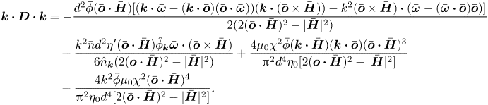 \begin{align} \boldsymbol{k} \boldsymbol{\cdot} \boldsymbol{D} \boldsymbol{\cdot} \boldsymbol{k} & ={-} \frac{d^{2} \bar{\phi} (\bar{\boldsymbol{o}} \boldsymbol{\cdot} \bar{\boldsymbol{H}}) [(\boldsymbol{k} \boldsymbol{\cdot} \bar{\boldsymbol{\omega}} - (\boldsymbol{k} \boldsymbol{\cdot} \bar{\boldsymbol{o}})(\bar{\boldsymbol{o}} \boldsymbol{\cdot} \bar{\boldsymbol{\omega}})) (\boldsymbol{k} \boldsymbol{\cdot} (\bar{\boldsymbol{o}} \times \bar{\boldsymbol{H}})) - k^{2} (\bar{\boldsymbol{o}} \times \bar{\boldsymbol{H}}) \boldsymbol{\cdot} (\bar{\boldsymbol{\omega}} - (\bar{\boldsymbol{\omega}} \boldsymbol{\cdot} \bar{\boldsymbol{o}}) \bar{\boldsymbol{o}})]}{2 (2 (\bar{\boldsymbol{o}} \boldsymbol{\cdot} \bar{\boldsymbol{H}})^{2} - |\bar{\boldsymbol{H}}|^{2})} \nonumber\\ &\quad - \frac{k^{2} \bar{n} d^{2} \eta^{\prime} (\bar{\boldsymbol{o}} \boldsymbol{\cdot} \bar{\boldsymbol{H}}) \hat{\phi}_{\boldsymbol{k}} \bar{\boldsymbol{\omega}} \boldsymbol{\cdot} (\bar{\boldsymbol{o}} \times \bar{\boldsymbol{H}})}{6 \hat{n}_{\boldsymbol{k}} (2 (\bar{\boldsymbol{o}} \boldsymbol{\cdot} \bar{\boldsymbol{H}})^{2} - |\bar{\boldsymbol{H}}|^{2})} + \frac{4 \mu_0 \chi^{2} \bar{\phi} (\boldsymbol{k} \boldsymbol{\cdot} \bar{\boldsymbol{H}})(\boldsymbol{k} \boldsymbol{\cdot} \bar{\boldsymbol{o}}) (\bar{\boldsymbol{o}} \boldsymbol{\cdot} \bar{\boldsymbol{H}})^{3}}{{\rm \pi}^{2} d^{4} \eta_0 [2 (\bar{\boldsymbol{o}} \boldsymbol{\cdot} \bar{\boldsymbol{H}})^{2} - |\bar{\boldsymbol{H}}|^{2}]} \nonumber\\ &\quad - \frac{4 k^{2} \bar{\phi} \mu_0 \chi^{2} (\bar{\boldsymbol{o}} \boldsymbol{\cdot} \bar{\boldsymbol{H}})^{4}}{{\rm \pi}^{2} \eta_0 d^{4} [2 (\bar{\boldsymbol{o}} \boldsymbol{\cdot} \bar{\boldsymbol{H}})^{2} - |\bar{\boldsymbol{H}}|^{2}]}. \end{align}
Here, the number density is expressed in terms of the volume fraction using the expression 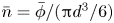 $\bar {n} = \bar {\phi } / ({\rm \pi} d^{3}/6)$. Equation (3.3) is used to express
  $\bar {\boldsymbol{o}} \times \bar {\boldsymbol{H}}$ in the first term on the right in (3.16):
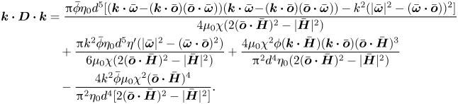 \begin{align} \boldsymbol{k} \boldsymbol{\cdot} \boldsymbol{D} \boldsymbol{\cdot} \boldsymbol{k} & = \frac{{\rm \pi} \bar{\phi} \eta_0 d^{5} [(\boldsymbol{k} \boldsymbol{\cdot} \bar{\boldsymbol{\omega}} \!-\! (\boldsymbol{k} \boldsymbol{\cdot} \bar{\boldsymbol{o}})(\bar{\boldsymbol{o}} \boldsymbol{\cdot} \bar{\boldsymbol{\omega}})) (\boldsymbol{k} \boldsymbol{\cdot} \bar{\boldsymbol{\omega}} \!-\! (\boldsymbol{k} \boldsymbol{\cdot} \bar{\boldsymbol{o}}) (\bar{\boldsymbol{o}} \boldsymbol{\cdot} \bar{\boldsymbol{\omega}})) - k^{2} (|\bar{\boldsymbol{\omega}}|^{2} - (\bar{\boldsymbol{\omega}} \boldsymbol{\cdot} \bar{\boldsymbol{o}}))^{2}]}{4 \mu_0 \chi (2 (\bar{\boldsymbol{o}} \boldsymbol{\cdot} \bar{\boldsymbol{H}})^{2} - |\bar{\boldsymbol{H}}|^{2})} \nonumber\\ &\quad + \frac{{\rm \pi} k^{2} \bar{\phi} \eta_0 d^{5} \eta^{\prime} (|\bar{\boldsymbol{\omega}}|^{2}-(\bar{\boldsymbol{\omega}} \boldsymbol{\cdot} \bar{\boldsymbol{o}})^{2})}{6 \mu_0 \chi (2 (\bar{\boldsymbol{o}} \boldsymbol{\cdot} \bar{\boldsymbol{H}})^{2} - |\bar{\boldsymbol{H}}|^{2})} + \frac{4 \mu_0 \chi^{2} \phi (\boldsymbol{k} \boldsymbol{\cdot} \bar{\boldsymbol{H}})(\boldsymbol{k} \boldsymbol{\cdot} \bar{\boldsymbol{o}}) (\bar{\boldsymbol{o}} \boldsymbol{\cdot} \bar{\boldsymbol{H}})^{3}}{{\rm \pi}^{2} d^{4} \eta_0 (2 (\bar{\boldsymbol{o}} \boldsymbol{\cdot} \bar{\boldsymbol{H}})^{2} - |\bar{\boldsymbol{H}}|^{2})} \nonumber\\ &\quad - \frac{4 k^{2} \bar{\phi} \mu_0 \chi^{2} (\bar{\boldsymbol{o}} \boldsymbol{\cdot} \bar{\boldsymbol{H}})^{4}}{{\rm \pi}^{2} \eta_0 d^{4} [2 (\bar{\boldsymbol{o}} \boldsymbol{\cdot} \bar{\boldsymbol{H}})^{2} - |\bar{\boldsymbol{H}}|^{2}]}. \end{align}
The diffusion coefficient extracted from this equation is of the form (2.39), where  $\boldsymbol{D}^{h}$ and
  $\boldsymbol{D}^{m}$ are
 \begin{equation} \left.\begin{gathered} \boldsymbol{D}^{h} = \frac{ ({{\boldsymbol{e}}_{\bar{\boldsymbol{\omega}}}} - \bar{\boldsymbol{o}}(\bar{\boldsymbol{o}} \boldsymbol{\cdot} {{\boldsymbol{e}}_{\bar{\boldsymbol{\omega}}}})) ({{\boldsymbol{e}}_{\bar{\boldsymbol{\omega}}}} - \bar{\boldsymbol{o}} (\bar{\boldsymbol{o}} \boldsymbol{\cdot} {{\boldsymbol{e}}_{\bar{\boldsymbol{\omega}}}})) - \boldsymbol{I} (1 - ({{\boldsymbol{e}}_{\bar{\boldsymbol{\omega}}}} \boldsymbol{\cdot} \bar{\boldsymbol{o}}))^{2}}{4 \varSigma_i [2 (\bar{\boldsymbol{o}} \boldsymbol{\cdot} {{\boldsymbol{e}}_{\bar{\boldsymbol{H}}}})^{2} - 1]},\\ \boldsymbol{D}^{m} = \frac{2 \varSigma_i \chi^{{\ast}} (\bar{\boldsymbol{o}} \boldsymbol{\cdot} {{\boldsymbol{e}}_{\bar{\boldsymbol{H}}}})^{3} ({{\boldsymbol{e}}_{\bar{\boldsymbol{H}}}} \bar{\boldsymbol{o}} + \bar{\boldsymbol{o}} {{\boldsymbol{e}}_{\bar{\boldsymbol{H}}}})}{{\rm \pi}[2 (\bar{\boldsymbol{o}} \boldsymbol{\cdot} {{\boldsymbol{e}}_{\bar{\boldsymbol{H}}}})^{2} - 1]} - \frac{4 \varSigma_i \chi^{{\ast}} (\bar{\boldsymbol{o}} \boldsymbol{\cdot} {{\boldsymbol{e}}_{\bar{\boldsymbol{H}}}})^{4} \boldsymbol{I}}{{\rm \pi} [2 (\bar{\boldsymbol{o}} \boldsymbol{\cdot} {{\boldsymbol{e}}_{\bar{\boldsymbol{H}}}})^{2}- 1]}, \\ {D_i^{\prime}} = \frac{\eta^{\prime} (1 - ({{\boldsymbol{e}}_{\bar{\boldsymbol{\omega}}}} \boldsymbol{\cdot} \bar{\boldsymbol{o}})^{2})}{6 \varSigma_i [2 (\bar{\boldsymbol{o}} \boldsymbol{\cdot} {{\boldsymbol{e}}_{\bar{\boldsymbol{H}}}})^{2}-1]}. \end{gathered}\right\}\end{equation}
Here, the dimensionless ratio of the magnetic and hydrodynamic torques is
 \begin{equation} \varSigma_i = \frac{\mu_0 \chi |\bar{\boldsymbol{H}}|^{2}}{{\rm \pi} \eta_0 d^{3} |\bar{\boldsymbol{\omega}}|}, \end{equation}
and the scaled susceptibility per unit volume is
 \begin{equation} \chi^{{\ast}} = \frac{\chi}{d^{3}}. \end{equation}
In going from (3.5) to (3.6), we had made the approximation  $\bar {n} \chi \ll 1$. If this approximation is not made, then there is only one change in the diffusion coefficients:
  $\chi ^{\ast } (1 + \bar {n} \chi )$ should be substituted for
  $\chi ^{\ast }$ in the first term on the right in the expression for
  $\boldsymbol{D}^{m}$.
3.2. Steady state
The orthogonal basis vectors  $({{\boldsymbol {e}}_{\bar {\boldsymbol{\omega }}}}, {{\boldsymbol {e}}_\parallel }, {{\boldsymbol {e}}_\perp })$ in figure 3(b) are used for an oblique magnetic field, where
  ${{\boldsymbol {e}}_{\bar {\boldsymbol{\omega }}}}$ is along the vorticity,
  ${{\boldsymbol {e}}_\parallel }$ is perpendicular to the vorticity in the
  $\bar {\boldsymbol{\omega }}- \bar {\boldsymbol{H}}$ plane, and
  ${{\boldsymbol {e}}_\perp }$ is perpendicular to the
  $\bar {\boldsymbol{\omega }}- \bar {\boldsymbol{H}}$ plane. The unit vectors
  ${{\boldsymbol {e}}_\parallel }$ and
  ${{\boldsymbol {e}}_\perp }$ are defined in (2.54) and (2.55). The solution
  $\hat {o}_{\boldsymbol{H}}$ (see (2.53a,b)) has to be determined numerically in this case; this is in contrast to the permanent dipole in an oblique magnetic field where it is possible to obtain an analytical solution, (2.57). The solutions have been derived in Kumaran (Reference Kumaran2021a,Reference Kumaranb) for a spheroid. The solution
  $\hat {o}_{\boldsymbol{H}}^{2}$ for a spherical particle satisfies the cubic equation
 \begin{equation} 4 \varSigma_i^{2} \hat{o}_{\boldsymbol{H}}^{4} [1 - \hat{o}_{\boldsymbol{H}}^{2}] + [\hat{\omega}_{\boldsymbol{H}}^{2} - \hat{o}_{\boldsymbol{H}}^{2}] = 0, \end{equation}
where  $\hat {\omega }_{\boldsymbol{H}}$ and
  $\hat {o}_{\boldsymbol{H}}$ are defined in (2.53a,b).
In the limit  $\varSigma _i \gg 1$, the particle aligns along the magnetic field and
  $\hat {o}_{\boldsymbol{H}} \rightarrow 1$. As
  $\varSigma _i$ is decreased, there are steady stable solutions for the orientation vector for the parameter regimes
 \begin{align} \varSigma_i^{2} & > \frac{1 + 18 \hat{\omega}_{\boldsymbol{H}}^{2} - 27 \hat{\omega}_{\boldsymbol{H}}^{4} - \sqrt{(1 - \hat{\omega}_{\boldsymbol{H}}^{2})(1 - 9 \hat{\omega}_{\boldsymbol{H}}^{2})^{3}}}{32 \hat{\omega}_{\boldsymbol{H}}^{2}} \quad \mbox{for} \ 0 \leq \hat{\omega}_{\boldsymbol{H}}^{2} \leq \frac{1}{9}, \end{align}
 \begin{align} & > \frac{9 (1 - 3 \hat{\omega}_{\boldsymbol{H}}^{2})}{8} \quad \mbox{for} \ \frac{1}{9} \leq \hat{\omega}_{\boldsymbol{H}}^{2} \leq \frac{1}{3}, \end{align}
 \begin{align} & > 0 \quad \mbox{for} \ \hat{\omega}_{\boldsymbol{H}}^{2} \geq \frac{1}{3}. \end{align}
When the conditions (3.22)–(3.24) are not satisfied, there are stable limit cycles and possibly an unstable steady solution. The boundary between the steady and rotating solutions in the  $\varSigma _i- \hat {\omega }_{\boldsymbol{H}}$ parameter space is shown by the blue line in figure 6.
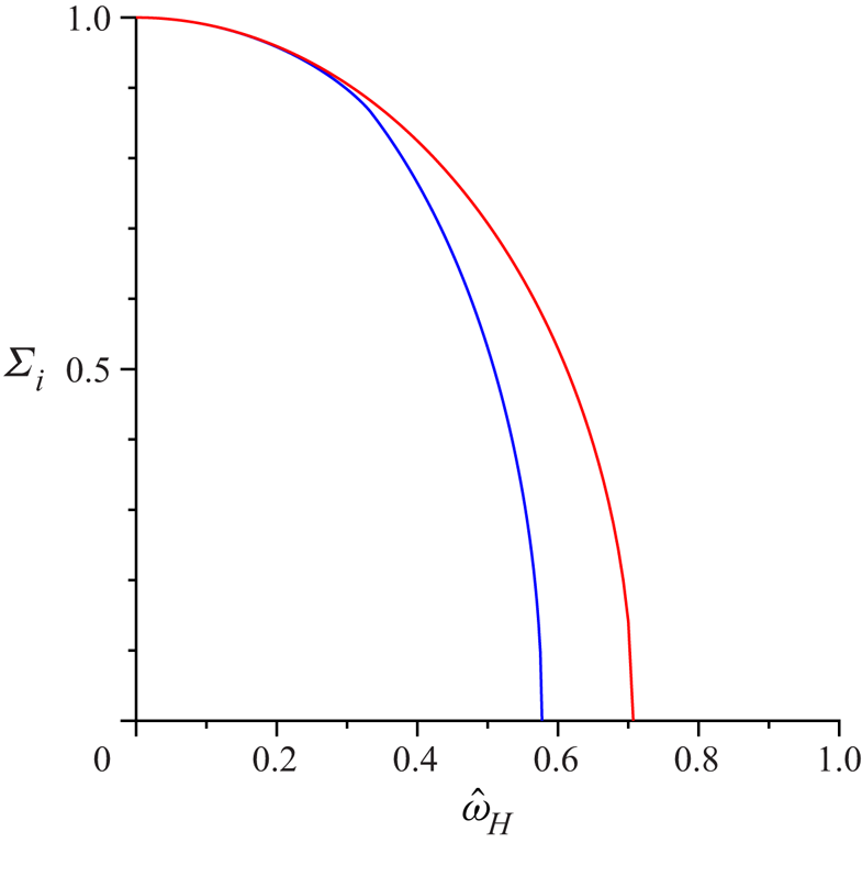
Figure 6. The boundary between the stable stationary solutions (above) and rotating states (below) for the single-particle dynamics, (3.24), is shown by the blue line, and the boundary for the dynamical transition at 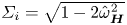 $\varSigma _i = \sqrt {1 - 2 \hat {\omega }_{\boldsymbol{H}}^{2}}$ is shown by the red line, in the
  $\hat {\omega }_{\boldsymbol{H}}- \varSigma _i$ plane.
The solutions of (3.21) for  $\bar {\boldsymbol{o}} \boldsymbol{\cdot } {{\boldsymbol {e}}_{\bar {\boldsymbol{H}}}}$ and the corresponding solutions of
  $\bar {\boldsymbol{o}} \boldsymbol{\cdot } {{\boldsymbol {e}}_{\bar {\boldsymbol{\omega }}}}$ are shown as functions of
  $\varSigma$ in figure 7. These are qualitatively different from those for particles with a permanent dipole shown in figure 2 because
  $\bar {\boldsymbol{o}} \boldsymbol{\cdot } {{\boldsymbol {e}}_{\bar {\boldsymbol{H}}}}$ is necessarily positive for an induced dipole; the parameter space
  $\bar {\boldsymbol{o}} \boldsymbol{\cdot } {{\boldsymbol {e}}_{\bar {\boldsymbol{H}}}} < 0$ does not exist in this case. The solutions for the orientation of a particle acted upon by a shear flow and a magnetic field are derived in orientation space consisting of the azimuthal and meridional angles of the particle orientation (Kumaran Reference Kumaran2021a,Reference Kumaranb). In this orientation space, the red lines in figure 7 are the unstable steady solutions, the blue lines are the stable steady solutions, and the brown lines are saddle points. The evolution of the fixed points for
  $0 < \hat {\omega }_{\boldsymbol{H}}^{2} < \tfrac {1}{9}$ is illustrated by the curve for
  $\hat {\omega }_{\boldsymbol{H}} = 0.1$ in figure 7. There is one stable fixed point for
  $\varSigma _i \gg 1$. As
  $\varSigma _i$ is decreased, one unstable fixed point and one saddle point appear in the phase diagram. When there is a further decrease in
  $\varSigma _i$, the saddle and stable fixed point merge, and there remain one unstable fixed point and one stable limit cycle. For
  $\frac {1}{9} < \hat {\omega }_{\boldsymbol{H}}^{2} < \frac {1}{3}$, the phase plot contains a stable fixed point and an unstable limit cycle for
  $\varSigma _i \gg 1$, and there is an exchange of stability to an unstable fixed point and a stable limit cycle for
  $\varSigma _i \ll 1$, as shown by the curve for
  $\hat {\omega }_{\boldsymbol{H}} = 0.5$ in figure 7. For
  $\frac {1}{3} < \hat {\omega }_{\boldsymbol{H}}^{2} < 1$, there is a stable fixed point that is aligned with the magnetic field for
  $\varSigma _i \gg 1$, and with the vorticity for
  $\varSigma _i \ll 1$.
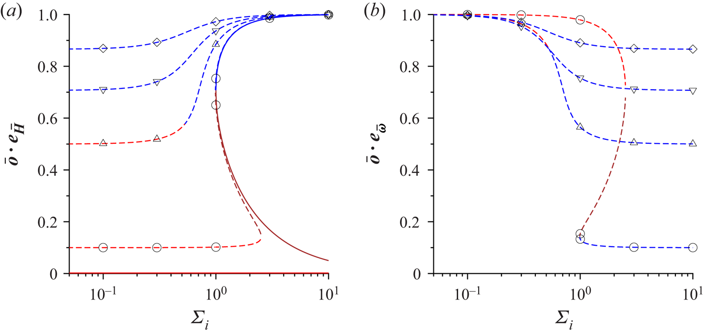
Figure 7. The variation of (a)  $\bar {\boldsymbol{o}} \boldsymbol{\cdot } {{\boldsymbol {e}}_{\bar {\boldsymbol{H}}}}$ and (b)
  $\bar {\boldsymbol{o}} \boldsymbol{\cdot } {{\boldsymbol {e}}_{\bar {\boldsymbol{\omega }}}}$ with
  $\varSigma _i$, for a particle with an induced dipole. The solid lines are the results for a parallel magnetic field
  ${{\boldsymbol {e}}_{\bar {\boldsymbol{\omega }}}} \boldsymbol{\cdot } {{\boldsymbol {e}}_{\bar {\boldsymbol{H}}}} = 0$, and the dashed lines are the results for an oblique magnetic field with
 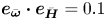 ${{\boldsymbol {e}}_{\bar {\boldsymbol{\omega }}}} \boldsymbol{\cdot } {{\boldsymbol {e}}_{\bar {\boldsymbol{H}}}} = 0.1$ (
 $\circ$),
  $\frac {1}{2}$ (
 $\triangle$),
  $\frac {1}{\sqrt {2}}$ (
 $\nabla$) and
  $\frac {\sqrt {3}}{2}$ (
 $\diamond$). The blue lines are the stable stationary nodes, the red lines are the unstable stationary nodes, and the brown lines are the saddle nodes. The value of
  ${{\boldsymbol {e}}_{\bar {\boldsymbol{\omega }}}} \boldsymbol{\cdot } {{\boldsymbol {e}}_{\bar {\boldsymbol{H}}}}$ for a parallel magnetic field is not shown in (b) because it is zero.
3.3. Parallel magnetic field
Equation (3.21) has analytical solutions when the magnetic field is parallel to the flow plane,  $\hat {\omega }_{\boldsymbol{H}} = 0$. The stable solution for the orientation vector exists only for
  $\varSigma _i > 1$, and the orientation vector is given by
 \begin{gather} \hat{o}_{\boldsymbol{H}} = \sqrt{\frac{1}{2} + \frac{\sqrt{\varSigma_i^{2} - 1}}{2 \varSigma_i}}, \quad \bar{\boldsymbol{o}} \boldsymbol{\cdot} {{\boldsymbol{e}}_\perp} = \sqrt{\frac{1}{2} - \frac{\sqrt{\varSigma_i^{2} - 1}}{2 \varSigma_i}},\end{gather}
 \begin{gather} 2 \hat{o}_{\boldsymbol{H}}^{2} - 1 = \frac{\sqrt{\varSigma_i^{2}-1}}{\varSigma_i}, \quad \hat{o}_{\boldsymbol{H}}(\bar{\boldsymbol{o}} \boldsymbol{\cdot} {{\boldsymbol{e}}_\perp}) = \frac{1}{2 \varSigma_i}. \end{gather}
 The orthogonal basis unit vectors  $({{\boldsymbol {e}}_{\bar {\boldsymbol{\omega }}}}, {{\boldsymbol {e}}_{\bar {\boldsymbol{H}}}}, {{\boldsymbol {e}}_\perp })$ shown in figure 3(a) are used, where
  ${{\boldsymbol {e}}_{\bar {\boldsymbol{\omega }}}}$ is along the vorticity direction,
  ${{\boldsymbol {e}}_{\bar {\boldsymbol{H}}}}$ is the along the direction of the magnetic field, and
  ${{\boldsymbol {e}}_\perp } = {{\boldsymbol {e}}_{\bar {\boldsymbol{\omega }}}} \times {{\boldsymbol {e}}_{\bar {\boldsymbol{H}}}}$. The diffusion coefficient due to hydrodynamic and magnetic interactions, (3.18), is reduced to the form in (2.47), where
 \begin{gather} {D_{\bar{\boldsymbol{\omega}} \bar{\boldsymbol{\omega}}}^{h}} = 0, \quad {D_{\bar{\boldsymbol{\omega}}\bar{\boldsymbol{\omega}}}^{m}} ={-} \frac{\chi^{{\ast}} \left(\varSigma_i + \sqrt{\varSigma_i^{2}-1}\right)^{2}}{{\rm \pi} \sqrt{\varSigma_i^{2}-1}}, \end{gather}
 \begin{gather}{D_{\bar{\boldsymbol{H}} \bar{\boldsymbol{H}}}^{h}} ={-} \frac{1}{4 \sqrt{\varSigma_i^{2}-1}}, \quad {D_{\bar{\boldsymbol{H}} \bar{\boldsymbol{H}}}^{m}} = 0, \end{gather}
 \begin{gather}{D_{\bar{\boldsymbol{H}} \perp}^{h}} = 0, \quad {D_{\bar{\boldsymbol{H}} \perp}^{m}} = \frac{\chi^{{\ast}} \left(\varSigma_i + \sqrt{\varSigma_i^{2}-1}\right)}{2 {\rm \pi}\sqrt{\varSigma_i^{2}-1}}, \end{gather}
 \begin{gather}{D_{{\perp}{\perp}}^{h}} ={-} \frac{1}{4 \sqrt{\varSigma_i^{2}-1}}, \quad {D_{{\perp}{\perp}}^{m}} ={-} \frac{\chi^{{\ast}} \left(\varSigma_i + \sqrt{\varSigma_i^{2}-1}\right)^{2}}{{\rm \pi} \sqrt{\varSigma_i^{2}-1}}. \end{gather}
The isotropic part of the diffusion tensor due to the concentration dependence of the viscosity and magnetic permeability is
 \begin{equation} {D_i^{\prime}} = \frac{\eta^{\prime}}{6 \sqrt{\varSigma_i^{2}-1}}. \end{equation}
 The asymptotic values of the diffusion matrix for  $\varSigma _i \gg 1$ and
  $\varSigma _i - 1 \ll 1$ are reported in table 1. The qualitative characteristics of the diffusion matrix are very similar to those for permanent dipoles in a parallel magnetic field discussed at the end of § 2.3. An important difference is that
  ${D_{\bar {\boldsymbol{\omega }}\bar {\boldsymbol{\omega }}}^{m}}$ and
  ${D_{\perp \perp }^{m}}$ diverge for
  $\varSigma _i \rightarrow 1$ where a transition occurs between static and rotating states.
The eigenvalues and eigenvectors of the diffusion matrix are provided in table 1. For the symmetric diffusion tensor, the eigenvalues are real, and the orthogonal eigenvectors are the principal axes of extension/compression. There is extension along directions with positive eigenvalues, indicating that concentration fluctuations are damped, and compression along directions with negative eigenvalues, resulting in amplification of concentration fluctuations. Planar aggregates perpendicular to the unstable direction are expected if two eigenvalues are positive and one is negative. If one eigenvalue is positive and two are negative, then cylindrical aggregates are expected to form aligned along the direction with positive eigenvalue. Spheroidal clusters are expected if all three directions are unstable, that is, all eigenvalues are negative. The eigenvalues in table 1 are calculated without including the isotropic component  ${D_i} \boldsymbol{I}$ in the diffusion tensor; that is, these do not include the effect of variations of viscosity with concentration. The eigenvectors are unchanged when the isotropic diffusion tensor with the viscosity correction is included, and the eigenvalues are transformed as
  $\lambda \rightarrow \lambda + {D_i}$.
The component  ${D_{\bar {\boldsymbol{\omega }}\bar {\boldsymbol{\omega }}}^{m}}$ of the diffusion tensor is always negative, and it diverges as
  $- 4 \chi ^{\ast } \varSigma _i/{\rm \pi}$ for
  $\varSigma _i \gg 1$. Therefore, perturbations are always unstable in the vorticity direction perpendicular to the flow, and there is clustering in this direction for a parallel magnetic field. For
  $\varSigma _i \gg 1$, the principal eigenvalues are aligned along the
  ${{\boldsymbol {e}}_{\bar {\boldsymbol{\omega }}}}, {{\boldsymbol {e}}_\parallel }, {{\boldsymbol {e}}_\perp }$ directions. The principal eigenvalue along the
  ${{\boldsymbol {e}}_\perp }$ direction diverges as
  $- 4 \chi ^{\ast } \varSigma _i / {\rm \pi}$. The principal eigenvalue along the
  ${{\boldsymbol {e}}_{\bar {\boldsymbol{H}}}}$ direction is positive/negative for
  $\chi ^{\ast } \gtrless {\rm \pi}$, and its magnitude decreases proportional
  $\varSigma _i^{-1}$ in this limit. Thus, depending on the value of
  $\chi ^{\ast }$, there is weak amplification/damping of fluctuations in the direction of the magnetic field, and strong amplification of fluctuations in the other two directions. When the magnetic field is perpendicular to the fluid velocity, this would result in the formation of long and narrow clusters aligned along the magnetic field.
For  $\varSigma _i - 1 \ll 1$ near the transition between rotating and steady states, all three eigenvalues diverge proportional to
  $(\varSigma _i - 1)^{-1/2}$. Two of the eigenvalues –
  $\lambda _3$ in the
  ${{\boldsymbol {e}}_\perp }$ direction, and
  $\lambda _2$ in the
  ${{\boldsymbol {e}}_{\bar {\boldsymbol{\omega }}}}- {{\boldsymbol {e}}_{\bar {\boldsymbol{H}}}}$ plane – are negative, therefore strong amplification of perturbations is predicted in these two directions. The other eigenvalue –
  $\lambda _1$ in the
  $\boldsymbol{e}_1$ direction – is positive/negative for
  $2 (\sqrt {2} - 1) \chi ^{\ast } \gtrless {\rm \pi}$, indicating damping of fluctuations if
  $\chi ^{\ast }$ exceeds a threshold. It should be noted that the divergence exponent
  $-\frac {1}{2}$ is a mean-field exponent, which could be altered if fluctuations are included.
3.4. Oblique magnetic field
The orthogonal coordinate system shown in figure 3(b) is used for an oblique magnetic field, where  ${{\boldsymbol {e}}_{\bar {\boldsymbol{\omega }}}}$ is along the direction of the vorticity perpendicular to the flow plane, the unit vector
  ${{\boldsymbol {e}}_\parallel }$ is perpendicular to
  ${{\boldsymbol {e}}_{\bar {\boldsymbol{\omega }}}}$ in the
  $\bar {\boldsymbol{\omega }}- \bar {\boldsymbol{H}}$ plane, and
  ${{\boldsymbol {e}}_\perp }$ is perpendicular to the
  $\bar {\boldsymbol{\omega }}- \bar {\boldsymbol{H}}$ plane. After the solution of (3.21) for
  $\hat {o}_{\boldsymbol{H}}$ is determined,
  $\bar {\boldsymbol{o}} \boldsymbol{\cdot } {{\boldsymbol {e}}_{\bar {\boldsymbol{\omega }}}}$ is calculated using (2.9). This specifies completely the orientation vector
  $\bar {\boldsymbol{o}}$. It is easily verified that for a parallel magnetic field with
  ${{\boldsymbol {e}}_{\bar {\boldsymbol{\omega }}}} \boldsymbol{\cdot } {{\boldsymbol {e}}_{\bar {\boldsymbol{H}}}} = 0$, the non-trivial solution reduces to (3.25a,b). The product
  $\bar {\boldsymbol{o}} \boldsymbol{\cdot } {{\boldsymbol {e}}_\parallel }$ is given by (2.58), and the product
  $\bar {\boldsymbol{o}} \boldsymbol{\cdot } {{\boldsymbol {e}}_\perp }$ is
 \begin{align} \bar{\boldsymbol{o}} \boldsymbol{\cdot} {{\boldsymbol{e}}_\perp} & = \frac{\bar{\boldsymbol{o}} \boldsymbol{\cdot} ({{\boldsymbol{e}}_{\bar{\boldsymbol{\omega}}}} \times {{\boldsymbol{e}}_{\bar{\boldsymbol{H}}}})}{\sqrt{1 - ({{\boldsymbol{e}}_{\bar{\boldsymbol{\omega}}}} \boldsymbol{\cdot} {{\boldsymbol{e}}_{\bar{\boldsymbol{H}}}})^{2}}} ={-} \frac{{{\boldsymbol{e}}_{\bar{\boldsymbol{\omega}}}} \boldsymbol{\cdot} (\bar{\boldsymbol{o}} \times {{\boldsymbol{e}}_{\bar{\boldsymbol{H}}}})}{\sqrt{1 - ({{\boldsymbol{e}}_{\bar{\boldsymbol{\omega}}}} \boldsymbol{\cdot} {{\boldsymbol{e}}_{\bar{\boldsymbol{H}}}})^{2}}} \nonumber\\ & = \frac{{{\boldsymbol{e}}_{\bar{\boldsymbol{\omega}}}} \boldsymbol{\cdot} (\boldsymbol{I} - \bar{\boldsymbol{o}} \bar{\boldsymbol{o}}) \boldsymbol{\cdot} {{\boldsymbol{e}}_{\bar{\boldsymbol{\omega}}}}}{2 \varSigma_i (\bar{\boldsymbol{o}} \boldsymbol{\cdot} {{\boldsymbol{e}}_{\bar{\boldsymbol{H}}}}) \sqrt{1 - \hat{\omega}_{\boldsymbol{H}}^{2}}} = \frac{\hat{o}_{\boldsymbol{H}}^{2} - \hat{\omega}_{\boldsymbol{H}}^{2}}{2 \varSigma_i \hat{o}_{\boldsymbol{H}}^{3} \sqrt{1 - \hat{\omega}_{\boldsymbol{H}}^{2}}}. \end{align}
Here, the torque balance equation (3.3) has been used to substitute for  $\bar {\boldsymbol{o}} \times {{\boldsymbol {e}}_{\bar {\boldsymbol{H}}}}$, and (2.9) is used to substitute
  $\hat {o}_{\boldsymbol{H}} = \hat {\omega }_{\boldsymbol{H}}/(\bar {\boldsymbol{o}} \boldsymbol{\cdot } {{\boldsymbol {e}}_{\bar {\boldsymbol{\omega }}}})$. Equations (2.58) and (3.32) are used to substitute for
  $\bar {\boldsymbol{o}}$ in (3.18) to obtain a diffusion matrix of the form (2.60). The elements of the matrix are listed in table 3, and the coefficients are plotted as a function of
  $\varSigma _i$ in figures 8 and 9.
Table 3. The asymptotic behaviour of the diffusion coefficients for  $\varSigma \gg 1$ and
  $\varSigma \ll 1$ for an oblique magnetic field for particles with induced dipoles.
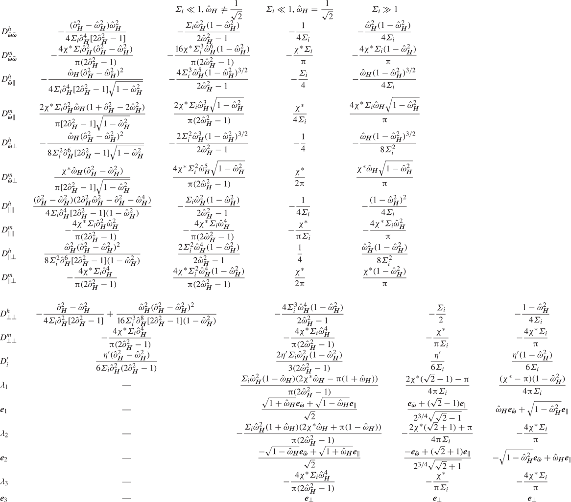
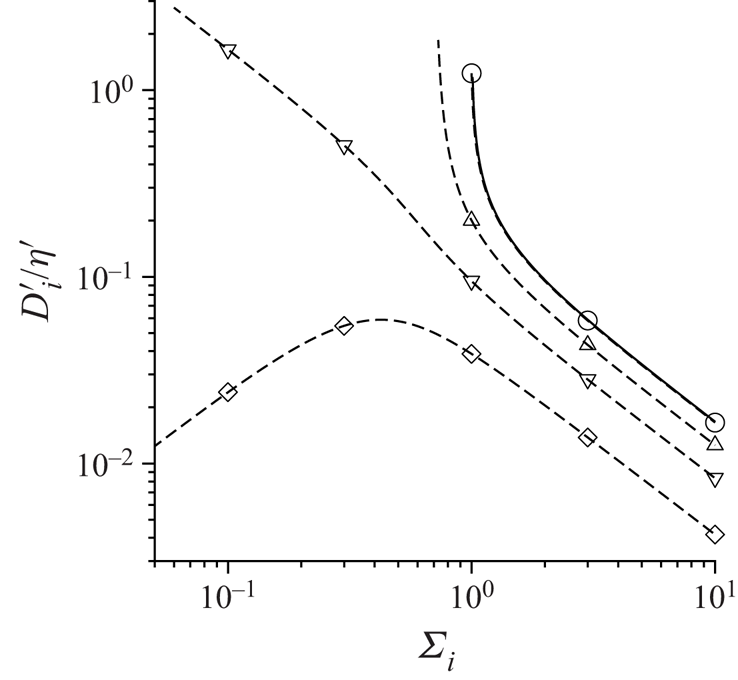
Figure 8. The scaled isotropic part of the diffusion tensor  ${D_i^{\prime }}/\eta ^{\prime }$ as a function of the parameter
  $\varSigma _i$ for particles with a induced dipole. Here,
  ${D_i^{\prime }}$ is given in (3.18). The orientations of the vorticity and magnetic field are
  ${{\boldsymbol {e}}_{\bar {\boldsymbol{\omega }}}} \boldsymbol{\cdot } {{\boldsymbol {e}}_{\bar {\boldsymbol{H}}}} = 0.1$ (
 $\circ$),
  $\frac {1}{2}$ (
 $\triangle$),
  $\frac {1}{\sqrt {2}}$ (
 $\nabla$) and
  $\frac {\sqrt {3}}{2}$ (
 $\diamond$). The solid line is the result for a parallel magnetic field.
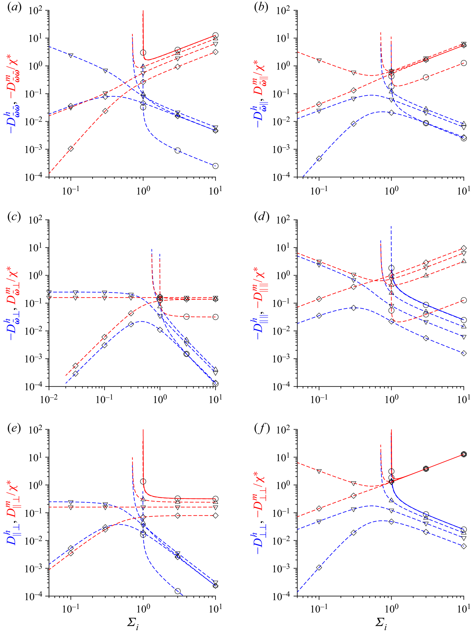
Figure 9. The components of the diffusion tensor: (a)  $- {D_{\bar {\boldsymbol{\omega }} \bar {\boldsymbol{\omega }}}^{h}}$ and
  $- {D_{\bar {\boldsymbol{\omega }}\bar {\boldsymbol{\omega }}}^{m}}/\chi ^{\ast }$, (b)
  $- {D_{\bar {\boldsymbol{\omega }} \parallel }^{h}}$ and
  ${D_{\bar {\boldsymbol{\omega }} \parallel }^{m}}/\chi ^{\ast }$, (c)
  $- {D_{\bar {\boldsymbol{\omega }} \perp }^{h}}$ and
  ${D_{\bar {\boldsymbol{\omega }} \perp }^{m}}/\chi ^{\ast }$, (d)
  $- {D_{\parallel \parallel }^{h}}$ and
  $- {D_{\parallel \parallel }^{m}}/\chi ^{\ast }$, (e)
  ${D_{\parallel \perp }^{h}}$ and
  ${D_{\parallel \perp }^{m}}/\chi ^{\ast }$, and (f )
  $- {D_{\perp \perp }^{h}}$ and
  $- {D_{\perp \perp }^{m}}/\chi ^{\ast }$, due to hydrodynamic interactions (blue lines) and magnetic interactions (red lines) as functions of the parameter
  $\varSigma _i$ for particles with an induced dipole moment. The orientations of the vorticity and magnetic field are
  ${{\boldsymbol {e}}_{\bar {\boldsymbol{\omega }}}} \boldsymbol{\cdot } {{\boldsymbol {e}}_{\bar {\boldsymbol{H}}}} = 0.1$ (
 $\circ$),
  $\frac {1}{2}$ (
 $\triangle$),
  $\frac {1}{\sqrt {2}}$ (
 $\nabla$) and
  $\frac {\sqrt {3}}{2}$ (
 $\diamond$). The solid blue and red lines are the non-zero results for a parallel magnetic field.
Also presented in table 3 are the expansions for the components of  $\boldsymbol{D}^{h}$ and
  $\boldsymbol{D}^{m}$ for the limits of small and large
  $\varSigma _i$, respectively. These are determined using the expansion for the solutions of (3.21):
 \begin{gather} \hat{o}_{\boldsymbol{H}} = \hat{\omega}_{\boldsymbol{H}} + 2 \varSigma_i^{2} \hat{\omega}_{\boldsymbol{H}}^{3} (1 - \hat{\omega}_{\boldsymbol{H}}^{2}) \quad \mbox{for} \ \varSigma_i \ll 1, \end{gather}
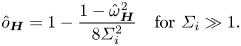 \begin{gather}\hat{o}_{\boldsymbol{H}} = 1 - \frac{1 - \hat{\omega}_{\boldsymbol{H}}^{2}}{8 \varSigma_i^{2}} \quad \mbox{for} \ \varSigma_i \gg 1. \end{gather}
The denominators of the diffusion coefficients in the third column of table 3 decrease to zero for  $\varSigma _i \ll 1$ and
  $\hat {\omega }_{\boldsymbol{H}} = \frac {1}{\sqrt {2}}$. In this case, it is necessary to first substitute (3.33) into the expressions in the second column of table 3, and then substitute
  $\hat {\omega }_{\boldsymbol{H}} = \frac {1}{\sqrt {2}}$ and take the limit
  $\varSigma _i \ll 1$. The results obtained in this manner are presented in the fourth column of table 3, and these are shown for different values of
  $\hat {\omega }_{\boldsymbol{H}}$ in figure 9.
The striking feature of the diffusion tensor elements in table 3 is the singularity at  $\hat {o}_{\boldsymbol{H}}^{2} = \frac {1}{2}$. From (3.21), this corresponds to
  $\varSigma _i = \sqrt {1 - 2 \hat {\omega }_{\boldsymbol{H}}^{2}}$, shown by the red line in figure 6, and this singularity exists only for
  $\hat {\omega }_{\boldsymbol{H}} < \frac {1}{\sqrt {2}}$. This boundary is different from the blue boundary between stationary and rotating states for the single-particle dynamics, and this represents a dynamical transition due to inter-particle interactions. At this boundary, the ‘susceptibility’ multiplying
  $\hat {o}^{{{\dagger}} }_{\boldsymbol{k}}$ in (3.11) decreases to zero, therefore the perturbation to the orientation vector
  $\hat {o}^{{{\dagger}} }_{\boldsymbol{k}}$ in (3.13) diverges. The divergence at
  $\hat {o}_{\boldsymbol{H}}^{2} = \frac {1}{2}$ is observed in all components of the diffusion tensor in figure 9, with the exception of
  ${D_{\perp \perp }^{m}}$. Of course, the analysis is not accurate at this point because it is carried out assuming
  $\hat {o}^{{{\dagger}} }_{\boldsymbol{k}} \ll 1$, and it is necessary to include nonlinear fluctuation effects in the vicinity of this point to extract the nature of the divergence. This is a subject for future study.
For  $\varSigma _i \gg 1$, the characteristics of the diffusion tensor are similar to those for dipolar particles in figure 5. The largest contributions to the diffusion tensor are
  ${D_{\bar {\boldsymbol{\omega }}\bar {\boldsymbol{\omega }}}^{m}}$,
  ${D_{\bar {\boldsymbol{\omega }} \parallel }^{m}}$,
  ${D_{\parallel \parallel }^{m}}$ and
  ${D_{\parallel \perp }^{m}}$; all of these diverge proportional to
  $\varSigma _i$. The eigenvalue
  $\lambda _3$ corresponding to the
  ${{\boldsymbol {e}}_\perp }$ direction is negative, and diverges proportional to
  $\varSigma _i$, therefore concentration fluctuations are amplified in the direction perpendicular to the plane containing the vorticity and magnetic field. In the
  ${{\boldsymbol {e}}_{\bar {\boldsymbol{\omega }}}}- {{\boldsymbol {e}}_\parallel }$ plane, one of the eigenvalues (
 $\lambda _2$) diverges proportional to
  $- (4 \chi \varSigma _i/{\rm \pi} )$, indicating strong amplification of concentration fluctuations in the
  $\boldsymbol{e}_2$ direction. The third eigenvalue (
 $\lambda _1$) decreases proportional to
  $\varSigma _i^{-1}$, and this is positive/negative for
  $\chi ^{\ast } \gtrless {\rm \pi}$, indicating weak amplification/damping of fluctuations. The two directions
  $\boldsymbol{e}_1$ and
  $\boldsymbol{e}_2$ align with
  ${{\boldsymbol {e}}_{\bar {\boldsymbol{H}}}}$ and
  ${{\boldsymbol {e}}_{\bar {\boldsymbol{\omega }}}}$ for a parallel magnetic field
  $\hat {\omega }_{\boldsymbol{H}} = 0$.
The characteristics of the diffusion tensor are similar to those for dipolar particles for  $\varSigma _i \ll 1$ and
  $\hat {\omega }_{\boldsymbol{H}} > \frac {1}{\sqrt {2}}$. The diffusion coefficients
  ${D_{\bar {\boldsymbol{\omega }} \bar {\boldsymbol{\omega }}}^{h}}$,
  ${D_{\bar {\boldsymbol{\omega }} \parallel }^{m}}$,
  ${D_{\parallel \parallel }^{h}}$,
  ${D_{\parallel \parallel }^{m}}$ and
  ${D_{\perp \perp }^{m}}$, and all three eigenvalues, decrease proportional to
  $\varSigma _i$. The eigenvalue of the diffusion tensor in the
  ${{\boldsymbol {e}}_\perp }$ direction is negative for
  $\hat {\omega }_{\boldsymbol{H}} > \frac {1}{\sqrt {2}}$,
  $\lambda _3 = - 4 \chi ^{\ast } \varSigma _i \hat {\omega }_{\boldsymbol{H}}^{2}/{\rm \pi} (2 \hat {\omega }_{\boldsymbol{H}}^{2}-1)$, and this is an unstable direction. One of the eigenvalues in the
  $\boldsymbol{e}_2$ direction is also always negative, while the third eigenvalue is positive/negative for
  $2 \chi ^{\ast } \hat {\omega }_{\boldsymbol{H}} \gtrless {\rm \pi}(1 + \hat {\omega }_{\boldsymbol{H}})$. Thus concentration fluctuations are unstable in the
  ${{\boldsymbol {e}}_\perp }$ and
  $\boldsymbol{e}_2$ directions, and they could be stable/unstable in the
  $\boldsymbol{e}_1$ direction depending on the value of
  $\chi ^{\ast }$.
For  $\hat {\omega }_{\boldsymbol{H}} > \frac {1}{\sqrt {2}}$, there is a dynamical transition at
  $\hat {o}_{\boldsymbol{H}} = \frac {1}{2}$ along the red line in figure 6. This is a transition in the collective dynamics of the particles, and is distinct from the single-particle transition between stationary and rotating states along the blue line in figure 6. All the coefficients of the diffusion matrix diverge proportional to
  $(\hat {o}_{\boldsymbol{H}} - \frac {1}{2})^{-1/2}$ at this transition. For
  $\hat {\omega }_{\boldsymbol{H}} = \frac {1}{\sqrt {2}}$, the elements of the diffusion tensor have a scaling different to that for
  $\hat {\omega }_{\boldsymbol{H}} > \frac {1}{\sqrt {2}}$. The elements
  ${D_{\bar {\boldsymbol{\omega }} \bar {\boldsymbol{\omega }}}^{h}}$,
  ${D_{\bar {\boldsymbol{\omega }} \parallel }^{m}}$,
  ${D_{\parallel \parallel }^{h}}$,
  ${D_{\parallel \parallel }^{m}}$ and
  ${D_{\perp \perp }^{m}}$ actually increase proportional to
  $\varSigma _i^{-1}$ in this limit. The eigenvalues of the diffusion matrix increase proportional to
  $\varSigma _i^{-1}$. Two of these are negative, therefore concentration fluctuations are amplified in one direction in the
  ${{\boldsymbol {e}}_{\bar {\boldsymbol{\omega }}}} - {{\boldsymbol {e}}_\parallel }$ plane and in the
  ${{\boldsymbol {e}}_\perp }$ direction. The third eigenvalue is positive for
  $2 \chi ^{\ast } (\sqrt {2} - 1) > {\rm \pi}$, and negative otherwise.
4. Conclusions
The principal result of the present calculation is that the hydrodynamic and magnetic inter-particle interactions manifest as an anisotropic diffusion tensor in the equation for the particle concentration field for spherical particles with a permanent or induced dipole moment. The magnetic dipole due to neighbouring particles results in the disturbance to the magnetic field at a test particle. When a neighbouring particle is stationary in a shear flow, there is a hydrodynamic disturbance in the form of an antisymmetric force moment, which causes a disturbance to the vorticity at the location of a test particle. In addition, there is the modification of the applied magnetic field due to the particle magnetisation, which depends on the particle concentration. The net effect of these disturbances is zero in a spatially uniform suspension. When there are variations in the particle concentration field, the net effect of these interactions in the torque balance equation results in a disturbance to the orientation vector. There is a force due to the gradient in the dot product of the magnetic moment and the magnetic field, which causes a drift velocity of the particles relative to the fluid. There is a contribution to the drift velocity due to the variation in the magnetic moment per unit volume when there is a concentration variation. The divergence of the drift velocity in the concentration equation has the form of an anisotropic diffusion term, and the elements of the diffusion tensor have been calculated for both permanent and induced dipoles.
The dimensionless parameters are the ratio of the magnetic and hydrodynamic torques on a particle,  $\varSigma$ for permanent dipoles (2.43) and
  $\varSigma _i$ for induced dipoles (3.19), and the ratio of the magnetic moment per unit volume and the magnetic field,
  ${M^{\ast }}$ (2.44) for permanent dipoles and
  $\chi ^{\ast }$ (3.20) for induced dipoles. The diffusion tensor consists of two distinct contributions, one due to magnetic interactions which is proportional to
  ${M^{\ast }}$ and
  $\chi ^{\ast }$, and the second due to hydrodynamic interactions, which does not depend on
  ${M^{\ast }}$ and
  $\chi ^{\ast }$. The product
  $\varSigma {M^{\ast }} = \mu _0 M^{2}/{\rm \pi} \eta _0 d^{6} |\bar {\boldsymbol{\omega }}|$, which is independent of the magnetic field, represents the effect of the interaction between particles and the modification of the magnetic field due to the particle magnetic moment. This is the inverse of the Mason number (Sherman et al. Reference Sherman, Becnel and Wereley2015), for simple shear flows where the magnitudes of the strain rate and vorticity are equal. For particles with an induced dipole moment, the product
  $\varSigma _i \chi ^{\ast } = \mu _0 \chi ^{2} |\bar {\boldsymbol{H}}|^{2}/{\rm \pi} \eta _0 d^{6} |\bar {\boldsymbol{\omega }}|$ is the inverse of the Mason number for a simple shear flow.
There are four ingredients that result in a net diffusion of the particles in a magnetic field under shear. These are the hydrodynamic disturbance, the magnetic disturbance, the disturbance to the particle orientation vector due to the interactions, and the modification of the field due to particle magnetic moment per unit volume. If the disturbance to the orientation vector is not included, then the diffusion coefficients are not predicted correctly. The interplay is subtle. For example, the term  $\unicode{x2460}$ in (2.35) is the interaction between the disturbance to the magnetic field and the undisturbed magnetic moment. This cancels out
  $\unicode{x2461}$ exactly, which is one of the terms due to the disturbance to the orientation. Thus some effects that are important in the absence of shear get cancelled out by the effect of the perturbation to the orientation vector in the presence of shear. All of these have to be correctly incorporated in the final expression for the force on the particles in order to predict the diffusion coefficients.
The components of the diffusion tensor are listed in table 1 for the particular case  $\hat {\omega }_{\boldsymbol{H}} = 0$ where the magnetic field is in the flow plane. For high magnetic field,
  $\varSigma, \varSigma _i \gg 1$, two principal directions of the diffusion tensor are along the magnetic field and along the vorticity direction (perpendicular to the flow plane), while the third component is orthogonal to the first two. For particles with permanent and induced dipoles, the eigenvalues of the diffusion tensor in the two directions perpendicular to the magnetic field are negative and diverge proportional to
  $\varSigma, \varSigma _i$; this would lead to strong amplification of concentration fluctuations in these two directions. The eigenvalue of the diffusion tensor along the magnetic field is positive when
  ${M^{\ast }}, \chi ^{\ast }$ exceed a threshold, and negative otherwise, and it decreases proportional to
  $\varSigma ^{-1}$; this would lead to weak amplification/damping of fluctuations along the direction of the magnetic field. When the magnetic field is perpendicular to the velocity, this explains the experimental observation of the formation of particle chains in the direction of the field direction when a magnetic field is applied.
The diffusion matrix exhibits interesting behaviour close to the transition between rotating and stationary solutions of the orientation vector,  $\varSigma - \frac {1}{2} \ll 1$ and
  $\varSigma _i - 1 \ll 1$. The component of the diffusion coefficient perpendicular to the plane of flow is negative, indicating amplification of concentration fluctuations perpendicular to the flow plane. The components of the diffusion tensor in the flow plane diverge proportional to
  $(\varSigma - \frac {1}{2})^{-1/2}$ and
  $(\varSigma _i - 1)^{-1/2}$ for permanent and induced dipoles. The eigenvalue of the diffusion matrix in one of the principal directions in the flow plane is negative, indicating strong clustering, while that in the other principal direction is positive when
  ${M^{\ast }}$ or
  $\chi ^{\ast }$ exceed a threshold. This implies a strong anisotropic clustering tendency in the flow plane as the magnetic field is reduced near the transition to rotating states. This intriguing phenomenon should be observable in experiments similar to those performed in the field of dynamical critical phenomena (Hohenberg & Halperin Reference Hohenberg and Halperin1977). The exponent
  $- \frac {1}{2}$ calculated here is a mean-field exponent; renormalisation group calculations are required to determine how this exponent changes when fluctuations are incorporated.
For a permanent dipole, there is no transition between rotating and stationary states for an oblique magnetic field ( $\hat {\omega }_{\boldsymbol{H}} \neq 0$). The elements of the diffusion tensor, and their asymptotic behaviour for
  $\varSigma \ll 1$ and
  $\varSigma \gg 1$, are shown in table 2. In all cases, one of the principal directions,
  ${{\boldsymbol {e}}_\perp }$, which is orthogonal to the vorticity and the magnetic field, and the eigenvalues of the diffusion matrix in this direction are all negative, indicating that there is strong amplification of concentration fluctuations in this direction when a magnetic field is applied. For particles with permanent dipoles in the limit
  $\varSigma \gg 1$, one eigenvalue of the diffusion tensor is negative and its magnitude increases proportional to
  $\varSigma$ in one principal direction in the
  $\bar {\boldsymbol{\omega }}- \bar {\boldsymbol{H}}$ plane, but the eigenvalue perpendicular to the
  $\bar {\boldsymbol{\omega }}- \bar {\boldsymbol{H}}$ plane is positive when
  ${M^{\ast }}$ exceeds a threshold and it decreases proportional to
  $\varSigma ^{-1}$. For
  $\varSigma \ll 1$, the eigenvalues in the
  $\bar {\boldsymbol{\omega }}- \bar {\boldsymbol{H}}$ plane increase proportional to
  $\varSigma$. One of the eigenvalues is negative, and the second could be positive or negative depending on the value of
  ${M^{\ast }}$.
For a suspension of particles with induced dipoles, there is a dynamical transition at the red line in figure 6, which is different from the blue line where there is a transition between static and rotating states in the single-particle dynamics. The dynamical transition is due to inter-particle interactions. Of course, the linearisation approximation is not applicable close to the transition where the disturbance to the orientation vector diverges, and more analysis is required to examine how the divergence in the diffusion coefficients is cut off due to nonlinear effects.
The eigenvalues of the diffusion matrix for particles with induced dipoles are similar qualitatively to those with permanent dipoles. For  $\varSigma _i \gg 1$, there is strong amplification of fluctuations perpendicular to the
  $\bar {\boldsymbol{\omega }}- \bar {\boldsymbol{H}}$ plane, and in one principal direction in the
  $\bar {\boldsymbol{\omega }}- \bar {\boldsymbol{H}}$ plane, and the magnitude of the eigenvalue increases proportional to
  $\varSigma _i$ in this limit. There is amplification or damping in the third direction depending on the value of
  $\chi ^{\ast }$, and the magnitude of the eigenvalue is proportional to
  $\varSigma _i^{-1}$. For
  $\varSigma _i \ll 1$, the magnitudes of the eigenvalues decrease proportional to
  $\varSigma _i$. The eigenvalue in the direction perpendicular to the
  $\bar {\boldsymbol{\omega }}- \bar {\boldsymbol{H}}$ plane is negative, and concentration fluctuations are amplified in this direction. The eigenvalue in one principal direction in the
  $\bar {\boldsymbol{\omega }}- \bar {\boldsymbol{H}}$ plane is also negative, and the second is positive or negative depending on the value of
  $\chi ^{\ast }$ and the angle
  $\hat {\omega }_{\boldsymbol{H}}$ between the magnetic field and the vorticity direction.
The effect of viscosity variations due to variations in the particle concentration has also been analysed, considering a linear model for the dependence of the viscosity on the concentration. This results in a positive contribution to the isotropic part of the diffusion tensor, which dampens concentration fluctuations. For particles with permanent dipoles, this contribution decreases proportional to  $\varSigma$ for
  $\varSigma \ll 1$, and proportional to
  $\varSigma ^{-1}$ for
  $\varSigma \gg 1$. For particles with induced dipoles, the diffusion coefficient decreases proportional to
  $\varSigma _i^{-1}$ for
  $\varSigma _i \gg 1$, and it decreases proportional to
  $\varSigma _i$ for
  $\varSigma _i \ll 1$ for values of
  $\hat {\omega }_{\boldsymbol{H}}$ where there is no dynamical transition.
The estimates for the hydrodynamic and magnetic contributions to the diffusion tensor are as follows. The hydrodynamic contribution operates perpendicular to the magnetic field for a parallel magnetic field (see (2.51a,b) and (3.30a,b)), and this scales as
 \begin{equation} D_h \sim \phi d^{2} |\bar{\boldsymbol{\omega}}|. \end{equation}
The characteristic diffusion time – the time for a particle to diffuse a distance comparable to its diameter – is  $\tau _h = (\phi |\bar {\boldsymbol{\omega }}|)^{-1}$, independent of particle diameter. The magnetic contribution is proportional to
  $D_m \sim \phi d^{2} |\bar {\boldsymbol{\omega }}| {M^{\ast }} \varSigma \sim \phi \mu _0 M^{2} / {\rm \pi}\eta d^{4}$ (see (2.49a,b)). This depends only on the magnetic moment of the particles, and not on the magnetic field or the particle angular velocity. The magnetic moment per particle is the product of the magnetic moment per unit volume
  $M_v$ and the particle volume,
  $M = M_v ({\rm \pi} d^{3}/6)\ \mbox {A}\ \mbox {m}^{2}$. Based on this, the estimate for the diffusion coefficient is
 \begin{equation} D_m \sim \phi d^{2} \mu_0 M_v^{2} / \eta. \end{equation}
The characteristic diffusion time, which is the time taken to diffuse a distance comparable to the particle diameter, is  $\tau _m = \eta / \phi \mu _0 M_v^{2}$. Thus both
  $D_h$ and
  $D_m$ are proportional to
  $d^{2} \phi$, and the characteristic diffusion times are independent of diameter, if
  $D_m$ is expressed in terms of magnetic moment per unit volume. The vorticity in magnetorheological applications, which is of the same magnitude as the strain rate, could vary between
  $1$ and
  $10^{4}\ \mbox {s}^{-1}$. Therefore, the minimum hydrodynamic diffusion time is
  $\tau _h \sim (10^{-4}/\phi )\ \mbox {s}$. For particles with a permanent magnetic dipole, the dipole moment is usually expressed as the magnetic moment per unit mass,
  $\textrm {emu}\ \textrm {g}^{-1}$, and the dipole moments are in the range 1–100
  $\textrm {emu}\ \textrm {g}^{-1}$. The magnetic moment per unit volume
  $M_v$ is the product of the magnetic moment per unit mass and the mass density, which is in the range
  $M_v \sim 1- 10^{3}\ \textrm {emu}\ \textrm {cm}^{-3} \sim 10^{3}- 10^{6}\ \mbox {A}\ \mbox {m}^{-1}$, if we assume that the material has mass density
  $1- 10\ \textrm {g}\ \textrm {cm}^{-3}$. Therefore, the minimum magnetic diffusion time is
  $(10^{-6}/\phi )\ \mbox {s}$. Thus the time required for a particle to diffuse across a distance comparable to its diameter is in the
  $\mbox {ms}- \mathrm {\mu } \mbox {s}$ range if the strain rate is sufficiently high. This provides a plausible mechanism for the formation of sample-spanning clusters when a magnetic field is applied.
The analysis of the diffusion due to interactions has been comprehensive, covering particle suspensions with permanent and induced dipoles, and different relative orientations of the flow and gradient directions and the applied magnetic field. The diffusion tensors determined here can be incorporated in continuum equations for magnetorheological fluids in order to capture the effect of interactions on the particle dynamics and orientation. They provide an opportunity for a more granular design of magnetorheological devices, where the dimensionless parameters and the relative orientation of the flow and magnetic field could be designed for dispersion/clustering of desired magnitudes along specific axes. From a fundamental perspective, the present analysis reveals a rich dynamical landscape inviting detailed inspection of several interesting phenomena, such as the divergence of the diffusivities at the transition between steady and rotating orientation states for a suspension of particles with a permanent dipole, and the dynamical transition where the diffusivities diverge due to collective effects for particles with an induced dipole. There is also scope for incorporating features such as spheroidal particles, where the shape factor could lead to additional interesting phenomena not present for spherical particles.
Funding
The author would like to thank the Department of Science and Technology, Government of India, for financial support through the grant JBR/2021/000021.
Declaration of interests
The author reports no conflict of interest.


 Open access