


1. Introduction
The canonical problem of liquid flows over superhydrophobic surfaces is concerned with an imposed shear over a single compound surface (Cottin-Bizonne et al. Reference Cottin-Bizonne, Barentin, Charlaix, Bocquet and Barrat2004). The simplest configuration comprises infinitely long slats of rectangular cross-section, arranged in a periodic array, with air bubbles trapped in the grooves separating them. The canonical shear-flow problem in that configuration may be reduced to two elementary subproblems: the longitudinal one, where the shear is applied parallel to the grooves, and the transverse one, where it applies perpendicular to them.
If the triple lines are pinned at the slat edges, the liquid domain interfaces the solid phase only at the top of the slats. The associated periodic geometry then depends upon two parameters, namely the solid fraction of the compound surface and the protrusion angle of the trapped bubbles (Davis & Lauga Reference Davis and Lauga2009b). In the case of flat menisci, the geometry depends upon a single parameter, the solid fraction. Using complex-analysis techniques in that idealised geometry, Philip (Reference Philip1972a,Reference Philipb) solved both the longitudinal and transverse problems, obtaining the slip length in closed form.
Extending Philip's calculations to non-zero protrusion angles requires either numerical simulations (Hyväluoma & Harting Reference Hyväluoma and Harting2008; Haase et al. Reference Haase, Wood, Lammertink and Snoeijer2016) or approximation schemes (Sbragaglia & Prosperetti Reference Sbragaglia and Prosperetti2007; Davis & Lauga Reference Davis and Lauga2009b). Of particular interest is the limit of small solid fractions. Since the imposed shear can only be supported by the solid boundary, the canonical problem is ill-posed at zero solid fraction. The limit of small solid fraction is accordingly a singular one (Schnitzer Reference Schnitzer2016). The scaling arguments of Ybert et al. (Reference Ybert, Barentin, Cottin-Bizonne, Joseph and Bocquet2007) suggest that the singularity is manifested in a slip length that diverges logarithmically with the solid fraction. Since significant superhydrophobic slippage is desirable in applications, liquid slippage at small solid fractions has been of interest in both experimental (Choi & Kim Reference Choi and Kim2006; Lee, Choi & Kim Reference Lee, Choi and Kim2008) and theoretical (Ybert et al. Reference Ybert, Barentin, Cottin-Bizonne, Joseph and Bocquet2007; Davis & Lauga Reference Davis and Lauga2009a, Reference Davis and Lauga2010; Crowdy Reference Crowdy2015) investigations, leading to extensive asymptotic analyses (Schnitzer Reference Schnitzer2016, Reference Schnitzer2017; Yariv Reference Yariv2017; Schnitzer & Yariv Reference Schnitzer and Yariv2018a,Reference Schnitzer and Yarivb; Yariv & Schnitzer Reference Yariv and Schnitzer2018).
Under sufficiently large pressure in the liquid phase, the meniscus is depinned from the edges of the slats and the liquid partially invades the grooves (Lee & Kim Reference Lee and Kim2009; Lv et al. Reference Lv, Xue, Shi, Lin and Duan2014); the slats then protrude into the liquid. Assuming flat menisci, as in Philip (Reference Philip1972a,Reference Philipb), the dimensionless geometry depends upon two geometric parameters, namely the ratios of the slat thickness and invasion depth to the period. The longitudinal and transverse problems in that geometry were both solved by Ng & Wang (Reference Ng and Wang2009) using eigenfunction expansions, allowing in principle for arbitrary values of the two governing parameters. Later on, Crowdy (Reference Crowdy2011) obtained an exact solution for the longitudinal problem based upon an analogy with irrotational flows.
It is desirable to supplement these exact solutions with closed-form approximations. To that end, Crowdy (Reference Crowdy2021) envisioned the limit of infinitely thin slats. The associated geometry – complementary, in a sense, to that considered by Philip – is again described by a single solid-fraction parameter, now given by the ratio of the slat protrusion to the period. The longitudinal problem in that complementary geometry was solved by Crowdy (Reference Crowdy2021) in closed form using a combination of radial slit and Möbius maps.
There is presently no comparable closed-form solution of the associated transverse problem. The limit of infinite protrusion was solved by Luchini, Manzo & Pozzi (Reference Luchini, Manzo and Pozzi1991) using the Wiener–Hopf method. This is a regular limit, where the slip length is finite when measured relative to the slat ends. We here address the transverse problem in the limit of small slat protrusion – the analogue to the small-solid-fraction limit in the classical geometries. The scaling arguments of Ybert et al. (Reference Ybert, Barentin, Cottin-Bizonne, Joseph and Bocquet2007) apply in the complementary geometry, suggesting that the slip length diverges logarithmically with vanishing slat protrusion. Our goal here is to systematically derive an asymptotic approximation that captures that slip-length singularity.
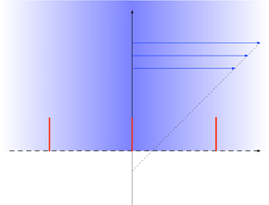
2. Problem formulation
The compound surface considered herein is formed by a  $2L$-periodic array of grooves, separated by infinitely thin slats. When immersed in a liquid (viscosity $\mu$), air is trapped in the grooves. We address the scenario where the meniscus, assumed flat, is displaced a distance $HL$ into the grooves.
Normalising all length variables by  $L$, we employ Cartesian coordinates $(x=x_1,y=x_2,x_3)$ with the plane $y=0$ coinciding with the menisci and the plane $x=0$ coinciding with one of the slats. The dimensionless geometry, of periodicity $2$ in the $x$-direction, is portrayed in figure 1. It is defined by a single parameter, the invasion depth $H$.
$H$.

Figure 1. Periodic boundary-value problem.
We consider here the case where the liquid is exposed to a shear flow, say of magnitude  $G$, applied perpendicular to the grooves. In analysing the flow problem, we normalise the fluid velocity by $GL$ and the stress variables by $\mu G$. The liquid velocity field is two-dimensional, say $\boldsymbol {u}=\hat {\boldsymbol {e}}_x u + \hat {\boldsymbol {e}}_y v$, where $u$ and $v$ are functions of $x$ and $y$. Neglecting the gas viscosity and the liquid inertia, the flow satisfies: (i) the continuity equation,
 \begin{equation} \frac{\partial u}{\partial x}+\frac{\partial v}{\partial y}=0 ; \end{equation}
(ii) the Stokes equation,
 \begin{equation} \boldsymbol{\nabla} p = \nabla^2\boldsymbol{u}, \end{equation}
wherein  $p$ is the pressure, a function of $x$ and $y$; (iii) the impermeability and no-slip conditions at the solid–liquid interfaces,
 \begin{equation} u = v = 0 \quad \text{for} \ 0< y< H\quad \text{at} \ x=2n \quad (n \in \mathbb{Z}); \end{equation}
(iv) the impermeability and shear-free conditions at the menisci,
 \begin{equation} v = \frac{\partial u}{\partial y}=0 \quad \text{at} \ y=0; \end{equation}
and (v) the imposed shear condition,
 \begin{equation} u\sim y \quad \text{as} \ y\to\infty. \end{equation}
The far-field behaviour (2.5) can be refined to the two-term expansion,
 \begin{equation} u \sim y + \lambda + o(1) \quad \text{as} \ y\to\infty, \end{equation}
wherein  $\lambda$ is the slip length; see figure 1. This quantity of interest can depend only upon $H$.
$H$.
3. Symmetries and simplification
The continuity and Stokes equations are invariant under the following reflection about the  $x$-axis:
 \begin{equation} u(x,-y) = u(x,y), \quad v(x,-y) ={-}v(x,y), \quad p(x,-y) = p(x,y). \end{equation}
We find it convenient to extend the velocity field to negative  $y$-values using (3.1). With that extension, the free-surface conditions (2.4) become redundant, while the solid-slat conditions (2.3) apply over extended line segments of length $2H$:
$2H$:
 \begin{equation} u = v = 0 \quad \text{for} \ |y|< H\quad \text{at} \ x=2n \quad (n \in \mathbb{Z}). \end{equation}
The extended ‘fluid domain’ now consists of the entire  $xy$-plane, absent these segments. Note that (2.5) then implies that
 \begin{equation} u\sim{-}y \quad \text{as} \ y\to-\infty. \end{equation}
 It is evident that  $u$,
$u$,  $v$ and $p$ are periodic in the $x$-direction,
 \begin{equation} u(x+2,y) = u(x,y), \quad v(x+2,y) = v(x,y), \quad p(x+2,y) = p(x,y). \end{equation}
In addition, they satisfy the following symmetries, for all integer  $n$:
$n$:
 \begin{gather} u(n-x,y) = u(n+x,y), \quad v(n-x,y)={-}v(n+x,y), \quad p(n-x,y) = p(n+x,y). \end{gather}
The extended fluid domain is naturally decomposed into a sequence of unit cells of length 2. With no loss of generality we may take the  $n$th cell $(n \in \mathbb {Z})$ as that extending between the ‘sides’ $x=-1+2n$ and $x=1+2n$. Each cell then contains a single line segment. Following ideas introduced by Schnitzer (Reference Schnitzer2016), we now consider the force balance on one such cell. The shear flows (2.5) and (3.3) imply a uniform shear stress, of magnitude unity in the $x$-direction, acting on the unit-cell liquid. Combined, they result in a hydrodynamic force (per unit length in the $x_3$-direction) of magnitude $4\hat {\boldsymbol {e}}_x$. Given (3.4) and (3.5), the two sides do not deliver a net hydrodynamic force. We now recall that the Stokes equation (2.2) may be written as
 \begin{equation} \boldsymbol{\nabla}\boldsymbol{\cdot}\boldsymbol{\sigma}=\boldsymbol{0}, \end{equation}
wherein  $\boldsymbol {\sigma } = -p \boldsymbol{\mathsf{I}} + \boldsymbol {\nabla }\boldsymbol {u} + (\boldsymbol {\nabla }\boldsymbol {u})^{\dagger}$ is the stress tensor, in which $^{\dagger}$ denotes tensor transposition. With the stress being divergence-free, we conclude that, for any closed contour $\mathcal {C}$ encircling the line segment in the cell (and lying entirely in the unit-cell domain),
 \begin{equation} \oint_{\mathcal{C}} \mathrm{d} l \, \hat{\boldsymbol{n}} \boldsymbol{\cdot} \boldsymbol{\sigma} = 4\hat{\boldsymbol{e}}_x, \end{equation}
wherein  $\mathrm {d} l$ is a differential length element and $\hat {\boldsymbol {n}}$ is the outward unit normal.
Since condition (3.7) has been derived from the governing equations, it does not provide any independent information. Nonetheless, it is indispensable in the asymptotic analysis that follows.
4. Streamfunction formulation
It is convenient to employ the streamfunction, defined by
 \begin{equation} u = \frac{\partial \psi}{\partial y}, \quad v ={-}\frac{\partial \psi}{\partial x}, \end{equation}
whereby the continuity equation (2.1) is trivially satisfied. In terms of  $\psi$, the Stokes equation (2.2) yields the biharmonic equation,
 \begin{equation} \nabla^4\psi=0, \end{equation}
while the far-field conditions (2.5) and (3.3) become
 \begin{equation} \psi \sim{\pm}\frac{y^2}{2} \quad \text{as} \ y\to\pm\infty. \end{equation}
Recall that  $\psi$ is defined to within an arbitrary additive constant that can be chosen at will. Given (3.1) we may therefore posit, with no loss of generality, that $\psi$ is an odd function of $y$, that is,
 \begin{equation} \psi(x,-y) ={-}\psi(x,y). \end{equation}
The slat conditions (3.2) then read
 \begin{equation} \psi = \frac{\partial \psi}{\partial x} = 0 \quad \text{for} \ |y|< H\quad \text{at} \ x=2n \quad (n \in \mathbb{Z}). \end{equation}
5. Small protrusions
We now focus upon the small protrusion limit,  $H\to 0$. In that limit, the integral condition (3.7) represents an effective point force (stokeslet), of magnitude $-4\hat {\boldsymbol {e}}_x$, acting on the liquid at the ‘grid points’ $(2n,0)$. Thus, making use of the $(r,\theta )$ polar coordinates in the $xy$-plane, the requirement of a two-dimensional stokeslet at the origin is expressed as (Pozrikidis Reference Pozrikidis1992)
 \begin{equation} \psi \sim \frac{r\ln r}{\rm \pi}\sin\theta \quad \text{as} \ r\to0. \end{equation}
When applying a similar requirement at all grid points and accounting for the reflection symmetry (3.1), the far-field conditions (2.5) and (3.3) are trivially satisfied.
With conditions (3.2) no longer applicable, the fluid velocity is defined to within an arbitrary uniform velocity in the  $x$-direction (equivalently, the streamfunction is defined up to an additive multiple of $y$). That velocity is evidently related to $\lambda$; see (2.6).
We make use of the complex-variable representation of any solution to the biharmonic equation (Hasimoto & Sano Reference Hasimoto and Sano1980),
 \begin{equation} \psi = \operatorname{Im} \{\,f(z) + \bar z g(z)\}, \end{equation}
wherein  $z=x+\mathrm {i} y$, $f$ and $g$ are two analytic functions, and the overbar denotes complex conjugation. The complex velocity,
 \begin{equation} \mathcal{U}=u-\mathrm{i} v, \end{equation}
is then given by
 \begin{equation} \mathcal{U}(z) = f'(z) + \bar z g'(z) - \bar g(\bar z). \end{equation}
 In principle, all that is required is to find two analytic functions that represent a sequence of point forces of magnitude  $-4\hat {\boldsymbol {e}}_x$ at the grid points. Now, the analytic functions $f_s$ and $g_s$ corresponding to a single point force of magnitude $-4\hat {\boldsymbol {e}}_x$ at the origin are given by (Hasimoto & Sano Reference Hasimoto and Sano1980)
 \begin{equation} f'_s(z) = \frac{1}{2{\rm \pi}}\log z, \quad g_s(z) ={-}\frac{1}{2{\rm \pi}}\log z. \end{equation}
We can therefore write the complex velocity in the present problem as
 \begin{equation} \mathcal{U}(z) = \sum_{n={-}\infty}^\infty \{\,f'_s(z-2n) + (\bar z-2n) g'_s(z-2n) - \bar g_s(\bar z-2n)\} + \mathrm{const.}, \end{equation}
where the arbitrary complex constant represents the invariance of the flow problem under the addition of a uniform velocity.
Plugging (5.5a,b) into (5.6) gives
 \begin{equation} 2{\rm \pi}\,\mathcal{U}(z) = 2\operatorname{Re} \sum_{n={-}\infty}^\infty \log(z-2n) - \sum_{n={-}\infty}^\infty \frac{\bar z-2n}{z-2n} + \mathrm{const.} \end{equation}
We observe that (5.7) merely constitutes a formal representation: both series appearing therein diverge. Nonetheless, we can render it useful. We start by adding to it a complex ‘constant’, given by the (divergent) series  $\sum _{n=-\infty }^\infty 1$:
 \begin{equation} 2{\rm \pi}\,\mathcal{U}(z) = 2\operatorname{Re} \sum_{n={-}\infty}^\infty \log(z-2n) - \sum_{n={-}\infty}^\infty \left\{ \frac{\bar z-2n}{z-2n} -1\right\} +\mathrm{const.} \end{equation}
The second series is now convergent:
 \begin{equation} \sum_{n={-}\infty}^\infty \left\{ \frac{\bar z-2n}{z-2n} -1\right\} ={-}2\mathrm{i} y \sum_{n={-}\infty}^\infty \frac{1}{z-2n}. \end{equation}
To calculate it we make use of the Mittag–Leffler expansion of the cotangent (Carrier, Krook & Pearson Reference Carrier, Krook and Pearson2005),
 \begin{equation} {\rm \pi}\cot{\rm \pi} z=\frac{1}{z} + \sum_{n=1}^\infty \frac{2z}{z^2-n^2}, \end{equation}
which can be recast as (cf. Yariv & Kirk Reference Yariv and Kirk2021)
 \begin{equation} \cot\frac{{\rm \pi} z}{2} = \frac{2}{\rm \pi} \sum_{n={-}\infty}^\infty \frac{1}{z-2n}, \end{equation}
thus providing the series in (5.9).
To deal with the first series in (5.8) we integrate (5.11) term-by-term, again disregarding the issue of convergence, to obtain the formal result:
 \begin{equation} \log\sin\frac{{\rm \pi} z}{2} = \sum_{n={-}\infty}^\infty\log (z-2n) + \mathrm{const.} \end{equation}
Substituting (5.9)–(5.12) into (5.8) we obtain
 \begin{equation} \mathcal{U}=\frac{1}{\rm \pi}\ln\left|\sin\frac{{\rm \pi} z}{2} \right| +\frac{\mathrm{i} y}{2} \cot\frac{{\rm \pi} z}{2} +C , \end{equation}
wherein  $C$ is an arbitrary complex constant. This explicit form no longer involves divergent series and is therefore admissible. Indeed, we can directly verify that (5.13) satisfies all the conditions specified in the problem governing $\mathcal {U}$ and is accordingly the requisite solution. At large $y$ we readily find from (5.13) that $\mathcal {U}\sim y -{\rm \pi} ^{-1}\ln 2+C$, with an algebraically small error (that is, an error that is asymptotically smaller than some positive power of $1/y$). Comparing with (2.6) and (5.3), we conclude that
 \begin{equation} C = \lambda +\frac{\ln 2}{\rm \pi}. \end{equation}
 In what follows, we will need the refined version of (5.1). Considering the limit  $z\to 0$, (5.13) and (5.14) give
 \begin{equation} \mathcal{U} \sim \frac{\ln({\rm \pi} |z|)}{\rm \pi} + \frac{\mathrm{i} y}{{\rm \pi} z} + \lambda, \end{equation}
with an algebraically small error. Equivalently
 \begin{equation} u \sim \frac{\ln({\rm \pi} r)+\sin^2\theta}{\rm \pi} + \lambda, \quad v \sim{-}\frac{\sin\theta\cos\theta}{\rm \pi}, \end{equation}
for small  $r$. We thus find from (4.1a,b) and (4.4) that
 \begin{equation} \psi \sim \frac{\ln({\rm \pi} r) + {\rm \pi}\lambda}{\rm \pi} r \sin\theta \quad \text{as} \ r\to0. \end{equation}
In both (5.16a,b) and (5.17), the asymptotic error is algebraically small. Approximation (5.17) provides the refinement of (5.1) that is required in the asymptotic analysis that follows.
6. Inner analysis
In the terminology of asymptotic methods (Hinch Reference Hinch1991), the preceding analysis corresponds to a leading-order calculation in the ‘outer’ limit, where  $H\to 0$ with $r$ fixed. In that limit, which corresponds to the scale of the period, the solid protrusions appear as point singularities. In what follows, we consider the complementary leading-order calculation in the ‘inner’ limit, on the scale of a single protrusion. The inner problem accounts for the boundary conditions on the line segment, but does not directly account for the applied shear and the presence of other segments. Because of the underlying periodicity, it is sufficient to consider the segment at $x=0$. The limit process is accordingly specified as $H\to 0$ with $r/H$ fixed.
With  $r={\rm ord}(H)$ it is natural to define the stretched radial coordinate,
 \begin{equation} R = r/H. \end{equation}
We also define the stretched Cartesian coordinates,
 \begin{equation} X = y/H, \quad Y={-}x/H, \end{equation}
where, for reasons to become evident soon, we have rotated the axes by  $90^{\circ }$ relative to the $(x,y)$ system. The line segment is now situated on the $X$-axis, extending between $X=-1$ and $X=1$. The azimuthal angle, measured anticlockwise from the $X$-axis, is
 \begin{equation} \phi=\theta-{\rm \pi}/2. \end{equation}
The inner geometry is shown in figure 2.

Figure 2. Inner problem.
Given the stretching in (6.2a,b), it is natural to define
 \begin{equation} \varPsi(X,Y;H) = H^{{-}1}\psi(x,y;H). \end{equation}
In the inner geometry, the neighbouring slats are shifted to infinity and become immaterial. The extended fluid domain therefore becomes the entire  $XY$-plane, sans the line segment on the $X$-axis. In that domain, $\varPsi$ is governed by the biharmonic equation in the stretched coordinates,
 \begin{equation} \left(\frac{\partial ^2}{\partial X^2} + \frac{\partial ^2}{\partial Y^2}\right)^2\varPsi = 0. \end{equation}
In addition, it satisfies: (i) the symmetry condition (cf. (4.4)),
 \begin{equation} \varPsi({-}X,Y) ={-}\varPsi(X,Y); \end{equation}
(ii) impermeability and no-slip conditions on the line segment (cf. (4.5)),
 \begin{equation} \varPsi = \frac{\partial \varPsi}{\partial Y} = 0 \quad \text{for} \ {-}1< X<1 \quad \text{at} \ Y=0; \end{equation}
and (iii) the far-field condition,
 \begin{equation} \varPsi = O({R\ln R}) \quad \text{as} \ R\to\infty, \end{equation}
which is necessitated by (5.1).
We observe that  $\varPsi$ is governed by a homogeneous problem. It resembles the inner problem of Shintani, Umemura & Takano (Reference Shintani, Umemura and Takano1983), who analysed the two-dimensional flow past an ellipse at low Reynolds numbers (see also Kropinski, Ward & Keller Reference Kropinski, Ward and Keller1995). In solving that problem, Shintani et al. (Reference Shintani, Umemura and Takano1983) used elliptic cylinder coordinates. We note that their definition of these coordinates is predicated (see their (2.2)) upon a geometry where the ellipse major axis is aligned with the $x$-axis (in their notation). Our definition of the rotated axes $(X,Y)$ thus allows us to handle the line segment as a degenerate ellipse using a notation which resembles that of Shintani et al. (Reference Shintani, Umemura and Takano1983) to some extent.
In the present geometry, the elliptic coordinates are defined as
 \begin{equation} X= \cosh\xi\cos\eta, \quad Y = \sinh\xi\sin\eta. \end{equation}
The extended fluid domain is covered by  $\xi >0$ and $-{\rm \pi} <\eta <{\rm \pi}$. The coordinate curves $\xi =\text {const.}$ are a family of ellipses with foci at $(\pm 1,0)$. In particular, the line segment is $\xi =0$. At large $\xi$ we find from (6.9a,b) that $R \sim {{\rm e}^\xi }/{2}$ and $\phi \sim \eta$, where the error is exponentially small (that is, asymptotically smaller than any power of $\xi$). Equivalently,
 \begin{equation} \xi \sim \ln(2R), \quad \eta \sim \phi, \end{equation}
as  $R\to \infty$, where the error is algebraically small.
Expressed in terms of the elliptic coordinates, the biharmonic equation (6.5) becomes
 \begin{equation} \left(\frac{\partial ^2}{\partial \xi^2} + \frac{\partial ^2}{\partial \eta^2}\right) \left\{ \frac{1}{\cosh^2\xi-\cos^2\eta} \left(\frac{\partial ^2\varPsi}{\partial \xi^2} + \frac{\partial ^2\varPsi}{\partial \eta^2}\right) \right\} = 0. \end{equation}
The symmetry condition (6.6) now reads
 \begin{equation} \varPsi(\xi,{\rm \pi}-\eta) ={-}\varPsi(\xi,\eta), \end{equation}
while the segment conditions (6.7) are simplified to
 \begin{equation} \varPsi = \frac{\partial \varPsi}{\partial \xi} = 0 \quad \text{at} \ \xi=0. \end{equation}
The solution of the above homogeneous problem is
 \begin{equation} \varPsi = D \left(\xi \cosh \xi - \sinh\xi\right)\cos\eta, \end{equation}
wherein  $D$ is an arbitrary constant. In writing (6.14) we have excluded terms that are incompatible with (6.8).
Making use of (6.10) we find that
 \begin{equation} \varPsi \sim D\left[\ln (2R)-1\right]R\cos\phi \quad \text{as} \ R\to\infty, \end{equation}
where the error is algebraically small.
7. Asymptotic matching and slip length
Using the terminology of matched asymptotic expansions, we have at our disposal both the inner expansion (5.17) of the outer approximation and the outer expansion (6.15) of the inner approximation. Both expressions are consistent with the standard approach in asymptotic analyses (Hinch Reference Hinch1991), where distinct asymptotic orders are grouped according to powers of the small parameter, disregarding its logarithms.
The outer solution (5.17) is given up to an additive constant, which is related to the slip length  $\lambda$. The inner solution (6.14) is defined up to the multiplicative prefactor $D$. Both $\lambda$ and $D$ are now set by the requirement of asymptotic matching between the two solutions. Thus, comparing (5.17) with (6.15) using (6.4) yields $D=1/{\rm \pi}$ and
 \begin{equation} \lambda = \frac{1}{\rm \pi}\left( \ln \frac{2}{{\rm \pi} H} -1 \right). \end{equation}
It is evident from the solution scheme that the asymptotic correction to (7.1) is algebraically small in  $H$. Approximation (7.1) for the slip length in the small protrusion limit constitutes the key result of the present paper.
Recall that the diametric limit of deep protrusion was solved by Luchini et al. (Reference Luchini, Manzo and Pozzi1991) using the Wiener–Hopf method. (There is no free surface in their problem formulation, but that difference becomes immaterial in the said limit.) In the present terminology, they found
 \begin{equation} \lim_{H\to\infty} \{ \lambda + H \}= 0.1771314\ldots . \end{equation}
Note that  $\lambda + H$ is the slip length measured in a coordinate system where the $x$-axis coincides with the top of the slats. This is the natural system to use in the limit $H\to \infty$. Since the error in (7.1) is algebraically small, that result is unaffected by such an origin shift. Note that the limit $H\to \infty$ is regular, while the limit $H\to 0$ is singular.
An intriguing aspect of the partially invaded configuration has to do with different slip lengths in the longitudinal and transverse problems. Recall that, in the longitudinal case, Crowdy (Reference Crowdy2021) obtained the slip length (in the present notation)
 \begin{equation} \frac{2}{\rm \pi} \ln{\rm csch} \frac{{\rm \pi} H}{2}. \end{equation}
The small- $H$ expansion of (7.3), $(2/{\rm \pi} )\ln (2/{\rm \pi} H)$, is more than twice the transverse slip length (7.1). This should be contrasted with the well-known $2:1$ ratio between the longitudinal and transverse slip lengths, which holds at leading algebraic order in Philip's configurations (see Lauga & Stone Reference Lauga and Stone2003). The $2:1$ ratio is also ‘violated’ in the limit $H\to \infty$, where the longitudinal counterpart of (7.2) is (Richardson Reference Richardson1971)
 \begin{equation} \lim_{H\to\infty} \{ \lambda + H \} = \frac{\ln4}{\rm \pi} . \end{equation}
In the shifted coordinate system, the longitudinal slip length is more than twice the transverse value.
8. Concluding remarks
When using eigenfunction expansions in groove-array configurations, there is no fundamental difference between the respective analyses in the longitudinal and transverse problems (Ng & Wang Reference Ng and Wang2009). When attempting to obtain closed-form approximations, the situation is quite different. Since Laplace's equation is conformally invariant, the powerful methodology of complex analysis naturally fits the longitudinal problem. While the solution to the biharmonic equation does admit a complex-variable representation, it involves two analytic functions; finding them for a given geometry requires some ingenuity.
The difference is conspicuous in the geometry of partially invaded grooves: while the case of infinitely thin slats was solved in closed form in the longitudinal problem (Crowdy Reference Crowdy2021), no such solution exists in the transverse problem. Our asymptotic analysis, in the limit of small solid fractions, provides the first step in overcoming the gap between the two problems. Our key result is approximation (7.1) for the slip length. Following the proper procedure in asymptotic methods, logarithmically separated terms are grouped together, thus ensuring that the asymptotic error is algebraically small.
With an algebraically small error, it is anticipated that (7.1) would agree with numerical solutions of the exact problem at numerically small values of  $H$. Unfortunately, there is currently no available computational solution of the transverse problem at the idealised geometry of infinitely thin slats: the slat width appears as a parameter in the formulation of Ng & Wang (Reference Ng and Wang2009), with no computations carried out in their paper for zero width. (The smallest width employed in their illustrations is a tenth of the period.) With a finite width, the limit $H\to 0$ is no longer singular.
We note that the present asymptotic approach works, in principle, even for more complicated slat geometries. The outer problem would be unaltered, yielding the same matching condition (5.17). In the inner problem, one would need to solve the biharmonic equation with no slip on the (geometric extension of the) slat boundary and the same far-field condition (6.8). One would then, in general, extract from the solution the far-field behaviour (cf. (6.15))
 \begin{equation} \varPsi \sim \frac{\ln (2R)-\varLambda}{\rm \pi}R\sin\theta \quad \text{as} \ R\to\infty, \end{equation}
where  $\varLambda$ depends on the slat shape (with $\varLambda =1$ for the special case of a line segment considered here). Matching with (5.17) thus provides the requisite extension of (7.1),
 \begin{equation} \lambda = \frac{1}{\rm \pi}\left( \ln \frac{2}{{\rm \pi} H} -\varLambda \right). \end{equation}
The difficulty, of course, lies in the solution of the inner Stokes problem. When the assumption of infinitely thin slats is relaxed, that problem (extended about the real axis) involves a flow about a rectangular object, for which no tailored coordinates are available. Here, it may be advantageous to employ the Goursat representation together with a combination of Schwarz–Christoffel and Möbius transformations which map the exterior of the rectangular object to the exterior of the unit circle. It then remains to determine two analytic functions in that domain. Each of these functions can be represented as a combination of a logarithm (accounting for matching with (5.17)) and a Laurent series. This challenging direction is posed here as an open problem.
Funding
This work was supported by the US–Israel Binational Science Foundation (Grant No. 2020123).
Declaration of interests
The author reports no conflict of interest.


 Open access