


1. Introduction
Electrophoresis, characterized as the motion of charged particles suspended in a fluid medium under the action of externally applied electric fields (Saville Reference Saville1977; Anderson Reference Anderson1985; Ohshima Reference Ohshima1996, Reference Ohshima2006; Schnitzer et al. Reference Schnitzer, Zeyde, Yavneh and Yariv2013; Goswami et al. Reference Goswami, Dhar, Ghosh and Chakraborty2017; Ghosh, Mukherjee & Chakraborty Reference Ghosh, Mukherjee and Chakraborty2021) has been an important area of research over the decades owing to its key roles in separation and isolation processes (Ghosal Reference Ghosal2006; Westermeier Reference Westermeier2016), colloidal sciences (Ohshima Reference Ohshima2006) and DNA sorting (Kaigala et al. Reference Kaigala, Hoang, Stickel, Lauzon, Manage, Pilarski and Backhouse2008; Khair & Squires Reference Khair and Squires2009), as well as a host of other biochemical and medical diagnostic applications (Karger, Cohen & Guttman Reference Karger, Cohen and Guttman1989; Babnigg & Giometti Reference Babnigg and Giometti2004; Kremser, Blaas & Kenndler Reference Kremser, Blaas and Kenndler2004; Ramautar, Demirci & de Jong Reference Ramautar, Demirci and de Jong2006). Many of the earlier theoretical studies on this phenomenon, however, focus on the movement of uniformly charged particles in Newtonian liquids (Baygents & Saville Reference Baygents and Saville1991; Ohshima Reference Ohshima2006; Khair & Squires Reference Khair and Squires2009; Schnitzer & Yariv Reference Schnitzer and Yariv2012, Reference Schnitzer and Yariv2014; Schnitzer, Frankel & Yariv Reference Schnitzer, Frankel and Yariv2014) – a scenario that is often violated in many of the applications mentioned above. For instance, in entities such as proteins, DNA fragments and bacterial cells (Kremser et al. Reference Kremser, Blaas and Kenndler2004; Kaigala et al. Reference Kaigala, Hoang, Stickel, Lauzon, Manage, Pilarski and Backhouse2008; Westermeier Reference Westermeier2016), the surface charge is usually non-uniformly distributed (Anderson Reference Anderson1985). Additionally, non-uniformities in surface properties, including those in surface charge, may also be intentionally engineered in the form of ‘Janus particles’, often used as microprobes and solid surfactants (Zhang, Grzybowski & Granick Reference Zhang, Grzybowski and Granick2017). As such, Anderson and co-workers (Anderson Reference Anderson1985; Fair & Anderson Reference Fair and Anderson1989), among others (Yoon Reference Yoon1991; Velegol Reference Velegol2002; Hsu et al. Reference Hsu, Huang, Yeh and Tseng2012), have addressed electrophoretic mobility of non-uniformly charged particles, albeit exclusively in Newtonian fluids, and established that the linear and angular velocities of the particles are inevitably linked to the multipole moments of the surface charge distribution.
In many instances, however, electrophoretic motion occurs in a complex fluidic medium (Khair, Posluszny & Walker Reference Khair, Posluszny and Walker2012; Tang et al. Reference Tang, Liu, Guo, Liu and Jiang2014; Li & Koch Reference Li and Koch2020), wherein the suspending fluid itself exhibits non-Newtonian constitutive properties (Bird, Armstrong & Hassager Reference Bird, Armstrong and Hassager1987). For example, polymer gels such as agarose or polyacrylamide gels, often used in gel electrophoresis (Babnigg & Giometti Reference Babnigg and Giometti2004), exhibit strong viscoelastic characteristics (Bird et al. Reference Bird, Armstrong and Hassager1987), which include relaxation time scales, shear thinning and non-zero normal stress coefficients. In addition, it is well established that biological fluids such as blood and human saliva also demonstrate similar viscoelastic properties (Skalak, Ozkaya & Skalak Reference Skalak, Ozkaya and Skalak1989; Brust et al. Reference Brust, Schaefer, Doerr, Pan, Garcia, Arratia and Wagner2013) and electrically actuated motion in such fluids is becoming increasingly prominent (Zhao & Yang Reference Zhao and Yang2011, Reference Zhao and Yang2013; Kim et al. Reference Kim, Lee, Yoo and Kim2021; Mahapatra & Bandopadhyay Reference Mahapatra and Bandopadhyay2021; Kumar et al. Reference Kumar, Mukherjee, Sinha and Ghosh2022) owing to their important applications in emerging fields such as medical diagnostics (Lee et al. Reference Lee, Madou, Koelling, Daunert, Lai, Koh, Juang, Lu and Yu2001; Groisman, Enzelberger & Quake Reference Groisman, Enzelberger and Quake2003) and genomic sequencing (Alshareedah & Banerjee Reference Alshareedah and Banerjee2022). Despite this, electrophoretic motion in non-Newtonian fluids remains largely under-explored, with the notable exception of a few recent studies (Khair et al. Reference Khair, Posluszny and Walker2012; Posluszny Reference Posluszny2014; Choudhary et al. Reference Choudhary, Li, Renganathan, Xuan and Pushpavanam2020; Li & Koch Reference Li and Koch2020; Ghosh et al. Reference Ghosh, Mukherjee and Chakraborty2021). While some of these investigations tend to use power-law or Carreau-type constitutive models (Bird et al. Reference Bird, Armstrong and Hassager1987; Hsu, Yeh & Ku Reference Hsu, Yeh and Ku2006; Hsu & Yeh Reference Hsu and Yeh2007; Khair et al. Reference Khair, Posluszny and Walker2012), others have aptly used more robust differential viscoelastic models such as the Oldroyd-B model (Ghosh et al. Reference Ghosh, Mukherjee and Chakraborty2021) or the Giesekus model (Li & Koch Reference Li and Koch2020), capable of representing the constitutive behaviour of polymeric fluids with greater accuracy. Li & Koch (Reference Li and Koch2020) establish that the electrophoretic velocity of a uniformly charged particle would slow down in a viscoelastic medium as compared to a Newtonian one, and the nonlinear rheology of the fluid forces the particle velocity to be dependent on its size. Ghosh et al. (Reference Ghosh, Mukherjee and Chakraborty2021), on the other hand, have shown that the Smoluchowski slip velocity (Ajdari Reference Ajdari1996) at the edge of the thin electrical double layer (EDL) surrounding a particle is altered fundamentally when the suspending medium is viscoelastic. They derived general expressions for the resulting slip velocity for an arbitrarily but weakly charged particle, and subsequently used these to deduce the instantaneous electrophoretic mobility of non-uniformly but axisymmetrically charged particles in viscoelastic fluids. Experimental investigations on particle electrophoresis in viscoelastic media are even more scarce, with the exception of a few recent studies (Lu et al. Reference Lu, Patel, Zhang, Woo Joo, Qian, Ogale and Xuan2014, Reference Lu, DuBose, Joo, Qian and Xuan2015; Li & Xuan Reference Li and Xuan2018; Malekanfard et al. Reference Malekanfard, Ko, Li, Bulloch, Baldwin, Wang, Fu and Xuan2019), wherein intriguing physical outcomes such as streamwise particle oscillations and cross-stream migrations were reported.
It becomes clear from a close review of the literature that a comprehensive account of electrophoretic trajectories of particles carrying arbitrary non-uniform surface charge and suspended in a viscoelastic medium remains an important open question, despite its relevance to processes such as gel electrophoresis (Westermeier Reference Westermeier2016) that are used routinely in applications related to diagnostics and sample detection (Neoh et al. Reference Neoh, Tan, Sapri and Tan2019). The evolution of particle trajectories undoubtedly poses a non-trivial question, since non-axisymmetrically charged particles in general may undergo rotation, which in turn will actively alter the distribution of surface charge on the particle. Such effects, coupled with the non-Newtonian (and also nonlinear) constitution of the fluid may lead to intriguing and varied particle trajectories, with potential applications in particle sorting and separation processes. Indeed, previous studies on self-propelled Janus particles (Gomez-Solano, Blokhuis & Bechinger Reference Gomez-Solano, Blokhuis and Bechinger2016; Molotilin, Lobaskin & Vinogradova Reference Molotilin, Lobaskin and Vinogradova2016; Nosenko et al. Reference Nosenko, Luoni, Kaouk, Rubin-Zuzic and Thomas2020) do show that they may follow a wide spectrum of pathways, depending on the physical environment (such as the presence of a bounding surface nearby; Mozaffari et al. Reference Mozaffari, Sharifi-Mood, Koplik and Maldarelli2018) and the driving mechanics (such as diffusiophoresis; Das et al. Reference Das, Jalilvand, Popescu, Uspal, Dietrich and Kretzschmar2020). In the same spirit, it is natural to enquire whether similarly varied particle trajectories driven by an externally imposed electric field in complex fluidic media are also realizable, which may further bolster the already rich ensemble of applications of electrophoretic motion.
In view of the above, here we aim to develop a general semi-analytical asymptotic framework to construct electrophoretic trajectories in the thin EDL limit, of particles carrying a generic non-uniform surface charge, suspended in a viscoelastic medium whose constitutive relation is governed by the Oldroyd-B model. This particular constitutive model has been chosen to retain analytical tractability, without sacrificing the essential physics of viscoelasticity. The surface charge of the particle is assumed to be weak (defined later) but otherwise arbitrary, and ultimately this results in the flow being weakly viscoelastic (Li & Koch Reference Li and Koch2020; Ghosh et al. Reference Ghosh, Mukherjee and Chakraborty2021). We utilize the modified Smoluchowski slip velocity in viscoelastic fluids reported previously in the literature (Ghosh et al. Reference Ghosh, Mukherjee and Chakraborty2021), derived using a combination of singular and regular perturbation (Bender, Orszag & Orszag Reference Bender, Orszag and Orszag1999), and erect a regular asymptotic framework using the characteristic surface potential, wherein the first corrections to the particle's velocities (angular and translational) owing to the viscoelasticity of the suspending medium are computed using a juxtaposition of the generalized reciprocal theorem (Masoud & Stone Reference Masoud and Stone2019; Choudhary et al. Reference Choudhary, Li, Renganathan, Xuan and Pushpavanam2020) and the Lamb's general solutions (Happel & Brenner Reference Happel and Brenner2012). These velocities are used subsequently to compute the particle trajectories, accounting for the transformation of the surface charge distribution of the particle in a fixed laboratory reference frame during the course of its motion (see § 2). As applications of the general framework developed herein, we report representative particle trajectories as well as the temporal evolution of their migration and angular velocities, for several instances of (initially) non-axisymmetric surface charge distributions. At the same time, we also derive closed-form analytical solutions for the linear and angular velocities of the particle at specific instances, which are used to validate our framework by comparing them against results reported previously in the literature.
Our results reveal that viscoelasticity of the suspending medium may strongly influence the migration of non-uniformly charged particles normal to the direction of the applied electric field. We argue that the direction and the rate of this migration depend on the distribution of the surface charge, the particle size and the viscoelastic properties of the suspending medium. Our results establish further that a non-uniformly charged particle will undergo rotation until its dipole moment becomes collinear with the imposed field, and during the course of rotation, viscoelasticity of the surrounding medium can cause the particle to move perpendicular to the electric field by inducing interactions between the multipole moments of its surface charge. The ultimate steady-state motion in a viscoelastic medium is also governed by these interactions, and the migration then depends especially on the presence of quadrupole moments.
The rest of the paper is structured as follows. In § 2, we provide a basic description of the problem statement, the assumptions and the important characteristic scales. Section 3 outlines the fundamental governing equations and the asymptotic framework, which includes the leading-order (Newtonian) flow field and the generalized reciprocal theorem for deriving the first viscoelastic corrections. We also report some closed-form analytical solutions for the instantaneous particle velocities in this section. In § 4, we provide a concise outline of the particle trajectory computations. Section 5 showcases the representative particle trajectories as an application of the developed framework to some selective initial surface charge distributions. In § 6, a prospective experimental set-up is discussed to test the predictions from this work. Finally, we conclude in § 7.
2. Basic description of the system
2.1. Physical description of the system under consideration
Figure 1(a) shows a prototypical rigid and non-conducting spherical particle of radius  $a$, which bears an arbitrary non-uniform surface charge of density $\sigma '(\theta,\phi )$. The particle is suspended in a viscoelastic liquid obeying the Oldroyd-B constitutive relation, having viscosity $\mu$, permittivity $\epsilon$, relaxation time $\lambda _{1}'$ and retardation time $\lambda _{2}'$ (Bird et al. Reference Bird, Armstrong and Hassager1987). The surrounding liquid also contains dissolved electrolytes, which dissociate into their constituent ions and form an EDL around the particle's surface as shown in the schematic. The bulk electrolyte concentration away from the particle is assumed to be $c'_{0}$. For ease of computations that follow, we will use two sets of axes, as shown in the schematic. The first ( $r',\theta,\phi$ or $x',y',z'$) is stationary (laboratory-fixed axes), with its origin initially fixed at the particle centre. The second ( $\tilde {r}',\tilde {\theta },\tilde {\phi }$ or $\tilde {x}',\tilde {y}',\tilde {z}'$) is attached to the particle and hence undergoes rotation when the particle does so. Therefore, in this second frame of reference, the particle's surface charge distribution remains invariant during the course of its motion. Spherical coordinates of the stationary reference frame (i.e. the laboratory-fixed axis system) will be used to represent the relevant flow variables throughout this work, unless otherwise mentioned.

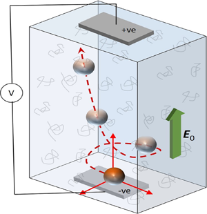
Figure 1. (a) Schematic of a spherical particle of radius  $a$ carrying arbitrary surface charge density $\sigma '(\theta,\phi )$, subjected to an externally applied electric field $E_0\hat {\boldsymbol{e}}_z$. The particle may translate with velocity $\boldsymbol{U}'$ and rotate with angular velocity $\boldsymbol \varOmega '$. The surrounding medium is viscoelastic with viscosity $\mu$, permittivity $\epsilon$, relaxation time $\lambda _{1}'$ and retardation time $\lambda _{2}'$, and obeys the Oldroyd-B constitutive relation. (b) Schematic representation of the electrophoretic trajectories traced out by particles similar to that described in (a), but carrying different types of surface charge distributions and/or having different sizes.
A steady electric field of magnitude  $E'_0$ (far field) is imposed in the $z$ direction. As a result, the particle moves with velocity $\boldsymbol{U}'$ – this translational velocity as well as its direction are a priori unknown and will have to be determined as part of the solution. At the same time, because of the non-uniformities in the surface charge, the particle may also rotate with angular velocity $\boldsymbol \varOmega '$ – once again, the magnitude and the direction of this angular velocity are a priori unknown and will be deduced with the solution. We emphasize here that because of rotation, the surface charge (or equivalently potential) on the particle will evolve continuously (although the intrinsic charge density in a particle fixed frame remains unchanged – see § 4.1), which in turn will also dynamically change $\boldsymbol{U}'$ and $\boldsymbol \varOmega '$. The translational velocity will propel the particle forward, while the angular velocity will dictate the charge distribution on its surface and hence govern the linear velocity. As a consequence, $\sigma '(\theta,\phi )$, $\boldsymbol{U}'$ and $\boldsymbol \varOmega '$ are all intricately coupled to one another, and this may result in fascinating particle trajectories, as we depict later.
2.2. The characteristic scales and an overview of the assumptions
2.2.1. The characteristic scales and the dimensionless parameters
For the present scenario, it will generally be insightful and convenient to work with dimensionless (unit-free) quantities, thus it is important to first consider the various characteristic scales and non-dimensional parameters that are relevant to the system under consideration. To this end, for any general variable, say  $\xi '$, we will denote the corresponding characteristic value as $\xi _{c}$.
Table 1 lists all the characteristic scales chosen for the present analysis. One important point to note here is that based on the characteristic surface charge ( $\sigma _c$, assumed to be a known quantity), we have defined a characteristic potential $\zeta _c$ – this potential indicates the order of magnitude of the ‘zeta potential’ on the particle surface. In other words, $\zeta _c$ gives an estimate of how much the potential drops across the diffuse part of the EDL. Thus both $\sigma _c$ and $\zeta _c$ quantify how strong the surface charge is on the particle. When a particle is uniformly charged, the choice of $\sigma _c$ is trivial; for non-uniformly charged particles, the surface average of $\sigma '(\theta,\phi )$ may be chosen as $\sigma _c$.
Table 1. Characteristic scales chosen (Saville Reference Saville1977; Ajdari Reference Ajdari1996) to non-dimensionalize pertinent variables, equations and the boundary conditions.

Based on the above characteristic scales, we may define several non-dimensional numbers that are relevant to the present analysis: (i) the non-dimensional EDL thickness  $\delta = \lambda _{D}/a$; (ii) the characteristic potential on the particle surface relative to the thermal potential (Ajdari Reference Ajdari1996; Ghosh et al. Reference Ghosh, Mukherjee and Chakraborty2021) $\bar {\zeta }_0 = e\zeta _{c} /kT$; (iii) the externally imposed field strength relative to the thermal potential (Saville Reference Saville1977) $\beta = eE_{0}a/kT$; (iv) the nominal Deborah number, which quantifies the extent of viscoelasticity (Bird et al. Reference Bird, Armstrong and Hassager1987; Ghosh et al. Reference Ghosh, Mukherjee and Chakraborty2021), $De = u_{c}\lambda _c/a$.
2.2.2. The key assumptions
The present analysis is predicated on a few assumptions that simplify the governing equations (discussed later), yet without sacrificing the essential physics. We discuss some of those main assumptions here.
First, we will assume the particle's surface charge density to be ‘weak’, which necessitates  $\bar {\zeta }_0 \ll 1$. Second, we will confine ourselves to the thin EDL limit, which mandates that the characteristic EDL thickness $\lambda _{D} = \sqrt {\epsilon k_b T/2e^2 c'_0}$ is small compared to the particle radius (Ajdari Reference Ajdari1995), i.e. $\delta \ll 1$ – this condition is usually satisfied for most particles that undergo electrophoretic motion. Third, the nominal Deborah number $De$ is assumed to remain $O(1)$ or less. However, because of the weak surface charge ( $\bar {\zeta }_0\ll 1$), the (dimensionless) velocity would scale as $O(\bar {\zeta }_0)$ and hence the effective Deborah number (Ghosh et al. Reference Ghosh, Mukherjee and Chakraborty2021) $De_{eff}$ will become $O(\bar {\zeta }_0 De)$ $\sim O(\bar {\zeta }_0) \ll 1$, which indicates that the flow is only weakly viscoelastic despite the nominal $De$ being $O(1)$. Fourth, the imposed electric field strength is assumed to be low to moderate, so that $\beta \sim O(1)$.
Fifth, the flow field is assumed to be quasi-steady – i.e. the angular and the translational velocities of the particle are governed by the instantaneous surface charge distribution. Since the true velocity in the surrounding fluid scales as  $O(\bar {\zeta }_0 u_c)$, the angular velocity of the particle is expected to scale as $\varOmega _c \sim \bar {\zeta }_0 u_c/a$, thus the time scale associated with the change in the surface charge distribution becomes $\varOmega _c^{-1} \sim a/\bar {\zeta }_0 u_c$. Therefore, for the quasi-static assumption to be satisfied, one must ensure that this time scale is large compared to the characteristic time scale of the fluid itself, i.e. $\varOmega _c^{-1} \gg \lambda _c$, which ultimately requires $De_{eff} \ll 1$ – this is consistent with the third assumption stated above. As a result, the flow can adjust to any change in the surface charge (or potential) distribution almost instantaneously. Sixth, we ignore the presence of depletion layer around the particle, hence the entire body of the suspending fluid is assumed to obey the same constitutive relation – such a paradigm has been used extensively in the existing literature (Afonso, Alves & Pinho Reference Afonso, Alves and Pinho2009; Choudhary et al. Reference Choudhary, Li, Renganathan, Xuan and Pushpavanam2020; Li & Koch Reference Li and Koch2020; Mahapatra & Bandopadhyay Reference Mahapatra and Bandopadhyay2021). Seventh, the flow field is assumed to be viscosity dominated on account of low Reynolds number.
Finally, it is also important to note the limitations of the Oldroyd-B model used herein (Bird et al. Reference Bird, Armstrong and Hassager1987). Although this constitutive model can be applied to relatively higher strain rates (as compared to ordered fluids) and is successful in capturing stress relaxation and normal stress coefficients to a reasonable extent, it nevertheless fails to account for shear-thinning behaviour and non-zero second normal stress coefficients exhibited by several polymeric fluids (Natu & Ghosh Reference Natu and Ghosh2021). In addition, the applicability of the Oldroyd-B model at extremely high stretching rates, as observed inside the EDL, also becomes questionable. Despite this, the Oldroyd-B model is extremely useful in developing insights into the multi-dimensional flows of complex fluids, because it rightfully captures the essential physics of viscoelastic flows, as is evident from its widespread use in the existing literature (Phan-Thien Reference Phan-Thien1983; Bird et al. Reference Bird, Armstrong and Hassager1987; Tan & Masuoka Reference Tan and Masuoka2005; Aggarwal & Sarkar Reference Aggarwal and Sarkar2008; Mukherjee & Sarkar Reference Mukherjee and Sarkar2011; Turkoz et al. Reference Turkoz, Lopez-Herrera, Eggers, Arnold and Deike2018).
3. The governing equations for fluid motion in the thin EDL limit
3.1. The equations of motion and the boundary conditions
In this subsection, we will outline the strategy to compute the instantaneous translational and angular velocities of a particle carrying arbitrarily varying (but known) surface charge density, which will be used later to trace the particle's trajectory. The fluid flow is governed by the continuity and the Cauchy momentum equations along with the Oldroyd-B constitutive model. We will start directly with their dimensionless forms, wherein the non-dimensional version of any variable, say  $\xi '$, is expressed as $\xi = \xi '/\xi _c$ – see § 2.2.1 for the characteristic scales. The governing equations thus appear as (Bird et al. Reference Bird, Armstrong and Hassager1987)
 $$\begin{gather} -\boldsymbol{\nabla} p + \boldsymbol{\nabla} \boldsymbol{\cdot} {\boldsymbol{\mathsf{\tau}}} = 0\quad \text{and}\quad \boldsymbol{\nabla} \boldsymbol{\cdot} \boldsymbol{v} = 0 , \end{gather}$$
 $$\begin{gather}{\boldsymbol{\mathsf{\tau}}} + De\,\lambda _1 \boldsymbol{\mathsf{T}} = 2\boldsymbol{\mathsf{D}} + 2\lambda _2\,De\,\boldsymbol{\mathsf{S}} , \end{gather}$$
where  $p$ is the pressure, $\boldsymbol{v}$ is the velocity field, ${\boldsymbol{\mathsf{\tau}}}$ is the viscous stress, $\boldsymbol{\mathsf{D}}$ is the strain rate tensor, and $\boldsymbol{\mathsf{T}}$ and $\boldsymbol{\mathsf{S}}$ are respectively the first convected derivatives (Bird et al. Reference Bird, Armstrong and Hassager1987) of the stress tensor ( ${\boldsymbol{\mathsf{\tau}}}$) and the strain rate tensor ( $\boldsymbol{\mathsf{D}}$). The first convected derivative of a second-rank tensor $\boldsymbol{\mathsf{A}}$ is expressed as $\boldsymbol{\mathsf{B}} = {{\rm D}\boldsymbol{\mathsf{A}}}/{{\rm D}t} - {(\boldsymbol{\nabla } \boldsymbol{v})}^{\rm T} \boldsymbol{\cdot } \boldsymbol{\mathsf{A}} - \boldsymbol{\mathsf{A}} \boldsymbol{\cdot } (\boldsymbol{\nabla } \boldsymbol{v})$. Detailed expressions for the various components of these convected derivatives in spherical coordinates have been included in the supplementary material available at https://doi.org/10.1017/jfm.2022.1002 (see § S1 therein). It is important to note that we have not differentiated explicitly between the solvent and polymeric stresses, and ${\boldsymbol{\mathsf{\tau}}}$ in the above denotes the total stresses in the fluid. In other words, ${\boldsymbol{\mathsf{\tau}}} = {\boldsymbol{\mathsf{\tau}}}^{S} + {\boldsymbol{\mathsf{\tau}}}^{P}$, where the superscripts $S$ and $P$ respectively denote contributions from the solvent and polymeric stresses (Li & Koch Reference Li and Koch2020). As such, ${\boldsymbol{\mathsf{\tau}}}^{S} = 2\mu ^{S}\boldsymbol{\mathsf{D}}$ and ${\boldsymbol{\mathsf{\tau}}}^{P} + \lambda _1 \boldsymbol{\mathsf{T}}^{P}= 2\mu ^{P}\boldsymbol{\mathsf{D}}$, where $\mu ^{P}$ is the polymer viscosity, $\mu ^{S}$ is the solvent viscosity, and $\boldsymbol{\mathsf{T}}^{P}$ represents the convected derivative of ${\boldsymbol{\mathsf{\tau}}}^{P}$. Then the retardation time ( $\lambda _2$) may be linked to the more fundamental quantity $\mathcal{C} = \mu ^{P}/\mu ^{S}$ (a measure of the polymer concentration) as (Li & Koch Reference Li and Koch2020; Ghosh et al. Reference Ghosh, Mukherjee and Chakraborty2021) $\mathcal{C} = \lambda _1/\lambda _2-1$.
The above equations have been written for thin EDLs, hence there are no body forces acting on the fluid. Instead, the entire effect of the body forces acting within the EDL will be accounted for by using a slip velocity at its edge, which for  $\delta \ll 1$ effectively lies on the particle surface at $r = 1$. Essentially, the body forces within the double layer originating from the externally imposed electric field generate a flow therein, which in turn drives the fluid in the outer electroneutral region (the bulk) through the modified Smoluchowski slip velocity at the edge of the EDL. As such, at any given instant, the velocity field in (3.1) is subjected to the following boundary conditions on the particle surface and the far field (Anderson Reference Anderson1985; Ghosh et al. Reference Ghosh, Mukherjee and Chakraborty2021):
 $$\begin{gather} \boldsymbol{v}(r=1,\theta,\phi) = \boldsymbol\varOmega \times \hat{\boldsymbol{e}}_r + \boldsymbol{U} +\boldsymbol{V}_{HS} , \end{gather}$$
 $$\begin{gather}\boldsymbol{v}(r\rightarrow \infty,\theta,\phi) = 0 , \end{gather}$$
where  $\boldsymbol{V}_{HS}$ refers to the modified Smoluchowski slip velocity in viscoelastic fluids. Ghosh et al. (Reference Ghosh, Mukherjee and Chakraborty2021) have previously evaluated a closed-form expression for $\boldsymbol{V}_{HS}$ for arbitrary distribution of surface charge, provided that the latter was ‘weak’ (see § 2.2.2). This modified slip velocity was reported as an asymptotic sequence in $\bar {\zeta }_0$ (the non-dimensional characteristic surface potential) and was derived using a combination of singular and regular asymptotic techniques (Leal Reference Leal2007). The core idea behind the derivation was to treat the EDL as a separate region with characteristic length scale $\delta$, which required a rescaling of many of the pertinent flow variables. In particular, it was shown that because of the high shear rates within the EDL, the polymers are strongly stretched and this leads to the normal stresses such as $\tau _{\theta \theta }$, $\tau _{\phi \phi }$ and $\tau _{\theta \phi }$ scaling as $O(\delta ^{-2})$ within the EDL, while the rest of the shear stress components scale as $O(\delta ^{-1})$. The asymptotically large magnitudes of the normal stresses were in stark contrast to Newtonian fluids, for whom they all scale as $O(1)$ within the EDL. As a consequence, the slip velocity at the edge of the EDL gets modified and shows dependence on the curvature of the particle as well as the derivatives of the surface charge density with respect to polar and azimuthal angles – this is again in stark contrast to what is observed in a Newtonian medium. The detailed expressions for $\boldsymbol{V}_{HS}$ for a given distribution of surface charge are specified later.
Note that in order to evaluate  $\boldsymbol{V}_{HS}$, one requires the externally imposed electric field ( $\boldsymbol{E}_{ext}$), which can be computed from the external potential $\varphi _{ext}$ as $\boldsymbol{E}_{ext} = -\boldsymbol{\nabla }\varphi _{ext}$, where $\varphi _{ext}$ satisfies (Ghosh et al. Reference Ghosh, Mukherjee and Chakraborty2021) $\nabla ^2 \varphi _{ext}=0$ subject to, $[\hat {\boldsymbol{e}}_r\boldsymbol{\cdot }\boldsymbol{\nabla } \varphi _{ext} ]_{r=1} = 0$ and $[\boldsymbol{\nabla } \varphi _{ext} ]_{r\rightarrow \infty } = -\beta \hat {\boldsymbol{e}}_z$. The solution for $\varphi _{ext}$ thus appears as
 \begin{equation} \varphi_{ext} ={-}\beta\left(r + \frac{1}{2r^2}\right)P_1(\eta), \end{equation}
where  $\eta$ = $\cos (\theta )$, and $P_{1}(\eta )$ is the Legendre polynomial of the first kind, of order 1.
The instantaneous translational and angular velocities of the particle ( $\boldsymbol{U}$ and $\boldsymbol \varOmega$, respectively) are a priori unknown, and these may be evaluated by carrying out a force and moment balance (about the origin) on the particle. In the limit of thin EDL, the net charge on an imaginary sphere of radius $r\sim 1+\delta$ with its surface lying just at the edge of the EDL is zero, hence the total moment around the origin and the net force acting on this imaginary sphere (particle plus the EDL) should also amount to zero (Ye et al. Reference Ye, Sinton, Erickson and Li2002; Chen & Keh Reference Chen and Keh2014) . Mathematically, these two conditions are expressed as
 \begin{equation} \int_{S_{p}} ({-}p\boldsymbol{\mathsf{I}}+{\boldsymbol{\mathsf{\tau}}}) \boldsymbol{\cdot} \hat{\boldsymbol{e}}_{r}\,{\rm d}S = 0\quad \text{and} \quad \int_{S_{p}} \hat{\boldsymbol{e}}_{r}\times ({\boldsymbol{\mathsf{\tau}}}\boldsymbol{\cdot}\hat{\boldsymbol{e}}_{r})\,{\rm d}S = 0. \end{equation}
The above integrations are effectively carried out over the particle surface  $S_p$, located at $r = 1$, to the leading order in $\delta$.
3.2. Asymptotic analysis for weakly charged particles
We reiterate that the weak surface charge limit entails (see § 2.2.2)  $\bar {\zeta }_0 \ll 1$. The surface charge on the particle may be written as $\sigma '(\theta,\phi ) = \sigma _c\,\breve {\zeta }(\theta,\phi )$, such that $\breve {\zeta }(\theta,\phi )\sim O(1)$ when $\sigma '\sim O(\sigma _c)$ – see table 1. It may then be shown (Ajdari Reference Ajdari1996) that the resulting dimensionless ‘zeta’ potential (potential on the particle surface) becomes $\psi \sim \bar {\zeta }_0\,\breve {\zeta }(\theta,\phi )$, such that $\psi \sim \bar {\zeta }_0$, as also stated earlier. For weakly charged particles, the flow variables in (3.1a) may now be expanded in an asymptotic series of $\bar {\zeta }_0$, the generic form of which reads (for any flow variable, say $\xi$)
 \begin{equation} \xi = \bar{\zeta}_0\xi_{1} + \bar{\zeta}_0^{2}\xi_{2} + \cdots.\end{equation}
Here,  $\xi$ may represent any variable of interest, such as $\boldsymbol{v}$, ${\boldsymbol{\mathsf{\tau}}}$, $\boldsymbol{U}$ or $\boldsymbol \varOmega$. We emphasize here that the expansion in (3.5) starts at $O(\bar {\zeta }_0)$ simply because for particles having zero surface charge (meaning $\bar {\zeta }_0 = 0$), no flow should take place. At the same time, it is also important to note that because of their nonlinear mathematical forms, the expansions for the convected derivatives ( $\boldsymbol{\mathsf{T}}$ and $\boldsymbol{\mathsf{S}}$) read as (see the supplementary material and the discussion after (3.1a))
 \begin{equation} (\boldsymbol{\mathsf{T}},\boldsymbol{\mathsf{S}}) = \bar{\zeta}_0^2(\boldsymbol{\mathsf{T}}_2,\boldsymbol{\mathsf{S}}_2) + \bar{\zeta}_0^3(\boldsymbol{\mathsf{T}}_3,\boldsymbol{\mathsf{S}}_3) + \cdots.\end{equation}
One may also interpret (3.5) as a regular asymptotic expansion in  $De_{eff}$ that is $O(\bar {\zeta }_0)$, since $De\sim O(1)$; this alternative expansion would appear as (for any generic variable $\xi$) $\xi = \bar {\zeta }_0(\xi _1 + De_{eff}\,\xi _2 + De_{eff}^2\,\xi _3 + \cdots )$, which reasserts the fact that the flow is indeed weakly viscoelastic. A consequence of using $De_{eff}$ in the expansion is that (3.5) is exactly equivalent to an ordered expansion around the Newtonian limit, carried out for an Oldroyd-B fluid. Hence all the $O(\bar {\zeta }_0)$ variables, i.e. the leading terms, will be identical to those for Newtonian flows.
In what follows, we will confine our attention to the leading order – the Newtonian flow field and the first viscoelastic correction, i.e. the  $O(\bar {\zeta }_0^2)$ contributions in the expansion (3.5). Although $\breve {\zeta }$ will in general evolve with time, the analysis of this section will assume it to be specified (but arbitrary). At the same time, it is important to note that there will also be $O(\delta )$ corrections to the particle velocity, owing to finite EDL thickness. However, when $\bar {\zeta }_0 \gg \delta$, the $O(\bar {\zeta }_0^2)$ corrections in the thin EDL limit would be far more dominant than the $O(\delta )$ contribution. Although for axisymmetric particles (where $\breve {\zeta } = \breve {\zeta }(\theta )$ only) it is possible to proceed to higher orders of corrections, for arbitrarily varying surface charge densities that may be non-axisymmetric, the equations become too cumbersome to be amenable to closed-form solutions. The leading-order problem at $O(\bar {\zeta }_0)$ may be solved using the Lamb's general solutions. However, resolving the detailed velocity field at $O(\bar {\zeta }_0^2)$ would perhaps require numerical tools. Since we are interested mainly in the particle's velocity and ultimately its trajectory, we can greatly simplify the calculations at $O(\bar {\zeta }_0^2)$ using the generalized reciprocal theorem (Masoud & Stone Reference Masoud and Stone2019), as shown later.
3.3. The modified Smoluchowski slip velocity,  ${V}$$_{HS}$


As stated earlier, a key element towards determining the mobility of the particle is the modified Smoluchowski slip velocity appearing in (3.2a). Following Ghosh et al. (Reference Ghosh, Mukherjee and Chakraborty2021),  $\boldsymbol{V}_{HS}$ may be expressed in an asymptotic series of $\bar {\zeta }_0$ as
 \begin{equation} \boldsymbol{V}_{HS} = \bar{\zeta}_0\,\boldsymbol{V}_{HS}^{(1)} + \bar{\zeta}_0^2\,\boldsymbol{V}_{HS}^{(2)} + \cdots,\end{equation}
where  $\boldsymbol{V}_{HS}^{(j)} = V_{HS,\theta }^{(j)}\,\hat {\boldsymbol{e}}_{\theta }$ + $V_{HS,\phi }^{(j)}\,\hat {\boldsymbol{e}}_{\phi }$, $j = 1,2$. The expressions for the components of the slip velocity at various orders are given by
 \begin{gather} V_{HS,\theta}^{(1)} ={-} \tfrac{3}{2}\beta\sqrt{1-\eta^{2}}\,\breve{\zeta}(\theta,\phi),\quad V_{HS,\phi}^{(1)} = 0, \end{gather}
 \begin{gather} V_{HS,\theta}^{(2)} = De\,(\lambda_{1} - \lambda_{2})\left[-\frac{9\eta \beta^2}{2(1- \eta^2)^{3/2}}\,\omega_{1}^{2} + \omega_{1}\left\{ \frac{3\beta\eta}{1-\eta^2}\,\varGamma_{1} - \frac{27\beta^2}{\sqrt{1-\eta^2}}\,\omega_{1,\eta} \right.\right.\nonumber\\ -\left.\left. \frac{3\beta}{\sqrt{1-\eta^2}}\,\omega_{2}\right\} + 3\beta \varGamma_{1}\omega_{1,\eta} - \frac{3\beta}{1-\eta^2}\,\chi_{1}\omega_{1,\phi} \right], \end{gather}
 \begin{gather} V_{HS,\phi}^{(2)} ={-}De\,(\lambda_1 - \lambda_2)\,\frac{3\beta \omega_1\omega_3}{\sqrt{1-\eta^2}}. \end{gather}
In the above,  $\omega _1 = \breve {\zeta }(\theta,\phi )\,Q_1(\eta )$, $Q_{1}(\eta ) = \frac {1}{2}(\eta ^{2}-1)$ is the Gegenbauer polynomial of order 1 (Leal Reference Leal2007), $\varGamma _1 = \varOmega _{y}^{(1)}\cos (\phi ) - \varOmega _{x}^{(1)}\sin (\phi )$ and $\omega _2 = \chi _{1,\phi } + \eta \varGamma _{1}/\sqrt {1-\eta ^2}$, where $\chi _1 = \varOmega _{z}^{(1)}\sqrt {1-\eta ^2} - \eta (\varOmega _{x}^{(1)}\cos (\phi )+\varOmega _{y}^{(1)}\sin (\phi ))$ and $\omega _3 = \sqrt {1-\eta ^2}\,\chi _{1,\phi}+$ $ {\eta \chi _1}/{\sqrt {1-\eta ^2}}$; further, $\omega _{1,\eta } = \partial \omega _1/\partial \eta$, $\omega _{1,\phi } = \partial \omega _1/\partial \phi$, and so on.
The  $O(\bar {\zeta }_0)$ slip velocity is identical to that of Newtonian fluids, while the viscoelastic corrections are embedded in the $O(\bar {\zeta }_0^2)$ slip velocity, and note from (3.8b) and (3.8c) that this correction does not contain any Newtonian contribution. A second salient feature of the $O(\bar {\zeta }_0^2)$ slip velocity is its dependence on the particle rotation from the previous order, i.e. on $\boldsymbol \varOmega _1$, the reason for which may be attributed to the variable velocity generated across the particle surface because of rotation about a given axis. As a result, the fluid is forced to move along the azimuthal direction, as is evident from a non-zero $V_{HS,\phi }^{(2)}$, and this will play a key role in altering particle trajectories, as we demonstrate later.
3.4. The leading-order problem
3.4.1. The flow field
By substituting (3.5) into (3.1), it is straightforward to derive the  $O(\bar {\zeta }_0)$ equations, which read ${\boldsymbol{\mathsf{\tau}}}_1 = 2\boldsymbol{\mathsf{D}}_1$, $-\boldsymbol{\nabla } p_{1} + \nabla ^2\boldsymbol{v}_1 = 0$ and $\boldsymbol{\nabla } \boldsymbol{\cdot }\boldsymbol{v}_1= 0$, subject to $\boldsymbol{v}_1(r = 1,\theta,\phi ) = \boldsymbol \varOmega _1 \times \hat {\boldsymbol{e}}_r + \boldsymbol{U}_1 +\boldsymbol{V}_{HS}^{(1)}$, where the expression for $\boldsymbol{V}_{HS}^{(1)}$ is specified in (3.8a). The force- and torque-free conditions at this order would translate into $\int _{S_{p}} (-p_1\boldsymbol{\mathsf{I}}+{\boldsymbol{\mathsf{\tau}}}_1) \boldsymbol{\cdot } \hat {\boldsymbol{e}}_{r}\,{\rm d}S = 0$ and $\int _{S_{p}} \hat {\boldsymbol{e}}_{r}\times ({\boldsymbol{\mathsf{\tau}}}_1\boldsymbol{\cdot }\hat {\boldsymbol{e}}_{r})\,{\rm d}S = 0$, from which $\boldsymbol{U}_1$ and $\boldsymbol \varOmega _1$ may be determined. The leading-order velocity may be represented using the Lamb's general solution (Pak & Lauga Reference Pak and Lauga2014) and reads
 \begin{align} \boldsymbol{v}_1 = \sum_{n=1}^{\infty}&\left[\boldsymbol{\nabla}\times\left(\boldsymbol{x} \varLambda_{-(n+1)}\right)+\boldsymbol{\nabla}\varPhi_{-(n+1)}-\frac{n-2}{2n(2n-1)}\, r^2\,\boldsymbol{\nabla}\mathcal{P}_{-(n+1)}\right.\nonumber\\ &\quad \left.{}+\frac{n+1}{n(2n-1)}\,\boldsymbol{x}\mathcal{P}_{-(n+1)}\right], \end{align}
where  $\varLambda _{-(n+1)}$, $\varPhi _{-(n+1)}$ and $\mathcal{P}_{-(n+1)}$ are solid harmonics of order $-n-1$, and $r = |\boldsymbol{x}|$. For instance, $\mathcal{P}_{-(n+1)}$ has the expression
 \begin{equation} \mathcal{P}_{-(n+1)} = r^{{-}n-1}\sum_{l=0}^{n}P^{l}_n(\eta)(A_{ln}\cos l\phi+\tilde{A}_{ln}\sin l\phi), \end{equation}
where  $P^{l}_n(\eta )$ is the associated Legendre polynomial of order $n$ and $l$. Expressions for the remaining solid harmonics have been provided in Appendix A, along with expanded expressions for the velocity components. The pressure is given by $p_1 = \sum _{n=1}^{\infty }\mathcal{P}_{-n-1}$. To systematically work out the unknown coefficients $A_{ln}$, $\tilde {A}_{ln}, \ldots$, the velocity on the particle's surface may be written as (Pak & Lauga Reference Pak and Lauga2014)
 \begin{equation} \boldsymbol{v}_1(r=1,\theta,\phi) = \sum_{l=0}^{\infty}(\boldsymbol{M}_{l}(\theta)\cos l\phi + \tilde{\boldsymbol{M}}_l(\theta)\sin l\phi), \end{equation}
where  $\boldsymbol{M}(\theta ) = D_l(\theta )\,\hat {\boldsymbol{e}}_r + E_l(\theta )\, \hat {\boldsymbol{e}}_{\theta } + F_l(\theta )\,\hat {\boldsymbol{e}}_{\phi }$ and $\tilde {\boldsymbol{M}}(\theta ) = \tilde {D}_l(\theta )\,\hat {\boldsymbol{e}}_r + \tilde {E}_l(\theta )\,\hat {\boldsymbol{e}}_{\theta } +$ $\tilde {F}_l(\theta )\,\hat {\boldsymbol{e}}_{\phi }$. Since these velocity components are known from the given boundary condition on the particle surface, one can deduce the coefficients $\boldsymbol{M}$ and $\tilde {\boldsymbol{M}}$ ( $l = 0,1,2,\ldots$), from which the unknown coefficients in (3.9) may be jotted down using the orthogonality of the associated Legendre polynomials and following the procedure outlined by Pak & Lauga (Reference Pak and Lauga2014). For instance, the coefficient $A_{ln}$ can be deduced as
 \begin{equation} A_{ln} = \frac{2n-1}{2}\,\frac{(2n+1)(n-l)!}{(n+1)(n+l)!}\int_{{-}1}^{1}\left[nD_{l} + \frac{\partial}{\partial \eta}(E_{l}\sin\theta) - \frac{l\tilde{F}_{l}}{\sin\theta}\right]P_{n}^{l}(\eta)\,{\rm d}\eta. \end{equation}
The other unknown coefficients may be determined from similar relations, and these have been included in Appendix A. A brief outline of the methodology to compute the functions  $\boldsymbol{M}$ and $\tilde {\boldsymbol{M}}$ has been provided in Appendix B.
3.4.2. The leading-order particle velocity
The leading-order particle velocities (translational and angular) may be determined by equating the net hydrodynamic drag and torque on the particle to zero. In terms of the solid harmonics, these force and torque balances may be expressed as (Happel & Brenner Reference Happel and Brenner2012)
 $$\begin{gather} \boldsymbol{F} ={-}4{\rm \pi}\,\boldsymbol{\nabla}(r^3\mathcal{P}_{{-}2}) = 0 , \end{gather}$$
 $$\begin{gather}\boldsymbol{T} ={-}8{\rm \pi}\,\boldsymbol{\nabla}(r^3\varLambda_{{-}2}) = 0. \end{gather}$$
The above two conditions yield  $A_{01} = A_{11} = \tilde {A}_{11} = 0$ for the force balance, and $C_{01} = C_{11} = \tilde {C}_{11} = 0$ for the torque balance – see also (A1b). Hence for a given surface charge distribution, these coefficients may be determined using the procedure described in § 3.4.1, and since they contain $\boldsymbol{U}_1$ and $\boldsymbol \varOmega _1$, those may be evaluated by equating the above coefficients to zero. Analytical examples for specific cases of surface charge distributions have been included in § 3.6.
3.5. The first viscoelastic corrections to the particle velocities
3.5.1. The generalized reciprocal theorem
The first viscoelastic corrections due to the polymeric stresses contribute at  $O(\bar {\zeta }_0^2)$. It is again straightforward to derive the governing equations and the boundary conditions at this order starting from (3.1), and they take the following forms: $\boldsymbol{\nabla } \boldsymbol{\cdot } {\boldsymbol{\mathsf{\Theta}}}_{2} + \boldsymbol{b}_{2} = 0$ and $\boldsymbol{\nabla }\boldsymbol{\cdot } \boldsymbol{v}_2 = 0$, where ${\boldsymbol{\mathsf{\Theta}}}_{2} = -p_2\boldsymbol{\mathsf{I}}+2\boldsymbol{\mathsf{D}}_2$ is the linear part of the stresses at $O(\bar {\zeta }_0^2)$, while $\boldsymbol{b}_2 = \boldsymbol{\nabla }\boldsymbol{\cdot }{\boldsymbol{\mathsf{\tau}}}_{2}^{exc}$ and ${\boldsymbol{\mathsf{\tau}}}_2^{exc}$ is the excess polymeric stresses at this order. It follows directly from (3.1b) that ${\boldsymbol{\mathsf{\tau}}}_{2}^{exc} = De\,(2\lambda _{2}\boldsymbol{\mathsf{S}}_{2} - \lambda _{1}\boldsymbol{\mathsf{T}}_{2})$ and thus ${\boldsymbol{\mathsf{\tau}}}_2 = 2\boldsymbol{\mathsf{D}}_2+{\boldsymbol{\mathsf{\tau}}}_{2}^{exc}$. Moreover, as a consequence of the regular asymptotic framework, $\boldsymbol{\mathsf{T}}_{2} = 2\boldsymbol{\mathsf{S}}_{2}$ and thus $\boldsymbol{b}_{2} = 2\,De\,(\lambda _2 - \lambda _1)(\boldsymbol{\nabla } \boldsymbol{\cdot } \boldsymbol{\mathsf{S}}_{2})$. On the particle surface, the velocity field satisfies $\boldsymbol{v}_2(r = 1,\theta,\phi ) = \boldsymbol \varOmega _2 \times \hat {\boldsymbol{e}}_r + \boldsymbol{U}_2 +\boldsymbol{V}_{HS}^{(2)}$, where $\boldsymbol{V}_{HS}^{(2)}$ has been specified in (3.8b) and (3.8c). The far-field condition remains unchanged from (3.2b).
The  $O(\bar {\zeta }_0^2)$ corrections to the particle velocities may be computed using the generalized reciprocal theorem (Masoud & Stone Reference Masoud and Stone2019), which does not require one to evaluate the complete velocity field at this order. To this end, we consider an auxiliary Stokes flow around a similar spherical particle in a Newtonian medium, wherein the total stress field and the body forces are denoted respectively as $\hat{{\boldsymbol{\mathsf{\Theta}}}}$ ( $= -\hat {p} \boldsymbol{\mathsf{I}}+2\hat {\boldsymbol{\mathsf{D}}}$, where $\hat {\boldsymbol{\mathsf{D}}}$ is the auxiliary strain rate tensor) and $\boldsymbol{\hat {b}}$. This auxiliary flow field would satisfy $\boldsymbol{\nabla } \boldsymbol{\cdot } \hat {{\boldsymbol{\mathsf{\Theta}}}} + \hat {\boldsymbol{b}} = 0$ and $\boldsymbol{\nabla } \boldsymbol{\cdot } \hat {\boldsymbol{v}} = 0$, where $\hat {\boldsymbol{v}}$ denotes the velocity field associated with the auxiliary flow. Assuming that $\hat {\boldsymbol{v}}$ vanishes far away from the particle and the stresses of the viscoelastic flow decay at a rate faster than $1/r^{2}$, the generalized reciprocal theorem boils down to (Masoud & Stone Reference Masoud and Stone2019; Li & Koch Reference Li and Koch2020; Ghosh et al. Reference Ghosh, Mukherjee and Chakraborty2021)
 \begin{equation} \int _{S_p} \hat{\boldsymbol{e}}_r\boldsymbol{\cdot}{\boldsymbol{\mathsf{\Theta}}}_{2} \boldsymbol{\cdot} \hat{\boldsymbol{v}} \,{\rm d}S - \int _{S_p} \hat{\boldsymbol{e}}_r \boldsymbol{\cdot} \hat{{\boldsymbol{\mathsf{\Theta}}}} \boldsymbol{\cdot} \boldsymbol{v}_{2} \,{\rm d}S = \int_{V} \boldsymbol{b}_{2} \boldsymbol{\cdot} \hat{\boldsymbol{v}} \,{\rm d}V - \int_{V} \hat{\boldsymbol{b}} \boldsymbol{\cdot} \boldsymbol{v}_{2} \,{\rm d}V .\end{equation}
In the above equation, the integrations on the left-hand side are carried out over the particle surface at  $r = 1$, and those on the right-hand side are carried out over the entire fluid domain. Hence on $S_{p}$, $\boldsymbol{v}_{2}$ in the second integral on the left-hand side becomes equal to $\boldsymbol{U}_{2} + \boldsymbol \varOmega _{2}\times \hat {\boldsymbol{e}}_{r} + \boldsymbol{V}_{HS}^{(2)}$. The following auxiliary flow fields have been chosen here: (i) to determine the particle's translational velocity ( $\boldsymbol{U}_2$), the flow generated by a sphere translating with velocity $\hat {\boldsymbol{e}}$ (unit magnitude, along an arbitrary direction) in a quiescent medium is chosen as the auxiliary flow; (ii) to deduce the particle's rotational velocity ( $\boldsymbol \varOmega _2$), we will consider as the auxiliary flow the velocity field of a sphere rotating with angular velocity $\hat {\boldsymbol{e}}$ in a quiescent Newtonian fluid. Therefore, in both the scenarios, $\hat {\boldsymbol{b}} = 0$.
We will first apply the reciprocal theorem to the leading-order problem, which we have already solved in § 3.4, to validate our choices. At this order,  $\boldsymbol{b}_{1} = 0$ and hence (3.14) simplifies (replace ${\boldsymbol{\mathsf{\Theta}}}_2$, $\boldsymbol{b}_2$ and $\boldsymbol{v}_2$, respectively, with ${\boldsymbol{\mathsf{\Theta}}}_1$, $\boldsymbol{b}_1 = 0$ and $\boldsymbol{v}_1$) to
 \begin{equation} \int _{S_p} \hat{\boldsymbol{e}}_r\boldsymbol{\cdot} {\boldsymbol{\mathsf{\Theta}}}_{1} \boldsymbol{\cdot} \hat{\boldsymbol{v}} \,{\rm d}S = \int _{S_p} \hat{\boldsymbol{e}}_r \boldsymbol{\cdot} \hat{{\boldsymbol{\mathsf{\Theta}}}} \boldsymbol{\cdot} \boldsymbol{v}_{1} \,{\rm d}S .\end{equation}
To determine the particle's translation velocity, we chose the auxiliary flow (i) as mentioned above, for which (Pozrikidis & Jankowski Reference Pozrikidis and Jankowski1997) the traction on the particle surface ( $r = 1$) is given by $\hat {\boldsymbol{e}}_r\boldsymbol{\cdot }\hat {{\boldsymbol{\mathsf{\Theta}}}} = -\frac {3}{2}\hat {\boldsymbol{e}}$. Now, on $S_{p}$, $\boldsymbol{v}_{1} = \boldsymbol{U}_{1} + \boldsymbol \varOmega _{1}\times \hat {\boldsymbol{e}}_{r} + \boldsymbol{V}_{HS}^{(1)}$ and $\hat {\boldsymbol{v}} = \hat {\boldsymbol{e}}$, whereas the force-free condition requires $\int _{S_p} {\boldsymbol{\mathsf{\Theta}}}_{1}\boldsymbol{\cdot } \hat {\boldsymbol{e}}_r \,{\rm d}S = 0$. As a consequence, (3.15) may be simplified directly to deduce $\boldsymbol{U}_1$ as
 \begin{equation} \boldsymbol{U}_{1} ={-}\frac{1}{4{\rm \pi}}\int_{Sp}\boldsymbol{V}_{HS}^{(1)}\,{\rm d}S .\end{equation}
On the other hand, the rotational velocity of the particle may be determined by considering the auxiliary flow (ii) stated earlier, so that the traction vector on the particle surface becomes (Pozrikidis & Jankowski Reference Pozrikidis and Jankowski1997)  $\hat {\boldsymbol{e}}_{r} \boldsymbol{\cdot } \hat {{\boldsymbol{\mathsf{\Theta}}}} = -3\hat {\boldsymbol{e}}\times \hat {\boldsymbol{e}}_{r}$, while on $S_p$, $\hat {\boldsymbol{v}} = \hat {\boldsymbol{e}}\times \hat {\boldsymbol{e}}_{r}$. The torque-free condition becomes $\int _{S_p} \hat {\boldsymbol{e}}_r\times ({\boldsymbol{\mathsf{\Theta}}}_{1}\boldsymbol{\cdot } \hat {\boldsymbol{e}}_r) \,{\rm d}S = 0$, hence (3.15) may be simplified to determine the expression for the particle's rotational velocity as
 \begin{equation} \boldsymbol{\varOmega}_{1} ={-}\frac{3}{8{\rm \pi}}\int_{0}^{2{\rm \pi}}{\rm d}\phi\int_{{-}1}^{1}{\rm d}\eta\,(\hat{\boldsymbol{e}}_{r}\times\boldsymbol{V}_{HS}^{(1)}). \end{equation}
This is identical to the expression derived by Ghosh et al. (Reference Ghosh, Mukherjee and Chakraborty2021). Remarkably, application of the reciprocal theorem demonstrates that the leading-order (Newtonian) contribution to the particle's translational velocity is simply the surface average of the Smoluchowski slip velocity, while the angular velocity is simply the average moment of the slip velocity around the particle centre.
3.5.2. Viscoelastic corrections using the reciprocal theorem
We now apply (3.14) to determine  $\boldsymbol{U}_2$ and $\boldsymbol \varOmega _2$. To this end, we recall that $\boldsymbol{b}_{2} = 2\,De\,(\lambda _2 - \lambda _1)(\boldsymbol{\nabla } \boldsymbol{\cdot } \boldsymbol{\mathsf{S}}_{2})$ (because $\boldsymbol{\mathsf{T}}_2 = 2\boldsymbol{\mathsf{S}}_2$, a consequence of linearization around the Newtonian solution using regular perturbation). The force-free condition at $O(\bar {\zeta }_0^2)$ reads (see (3.4a,b)) $\int _{S_p} ({\boldsymbol{\mathsf{\Theta}}} _2+{\boldsymbol{\mathsf{\tau}}}_2^{exc})\boldsymbol{\cdot }\hat {\boldsymbol{e}}_r\,{\rm d}S = 0$, and upon enforcing the expression for ${\boldsymbol{\mathsf{\tau}}}_2^{exc}$, it simplifies to
 \begin{equation} \int_{S_{p}}{\boldsymbol{\mathsf{\Theta}}}_{2} \boldsymbol{\cdot} \hat{\boldsymbol{e}}_{r}\,{\rm d}S ={-}\int_{S_{p}}2\,De\,(\lambda_2 - \lambda_1)\boldsymbol{\mathsf{S}}_{2}\boldsymbol{\cdot}\hat{\boldsymbol{e}}_{r}\,{\rm d}S. \end{equation}
To deduce  $\boldsymbol{U}_2$, we use the same auxiliary flow as outlined in § 3.5.1 (see the discussion prior to (3.16)), along with (3.18) and the boundary condition for $\boldsymbol{v}_2$ on $S_p$ to simplify (3.14), which yields
 \begin{align} \boldsymbol{U}_{2}\boldsymbol{\cdot}\hat{\boldsymbol{e}} ={-}\frac{1}{4{\rm \pi} }\,\hat{\boldsymbol{e}} \boldsymbol{\cdot}\int _{S_p} \boldsymbol{V}_{HS}^{(2)}\,{\rm d}S \!+ \frac{De}{3{\rm \pi}}\,(\lambda_2 - \lambda_1)\left\{ \hat{\boldsymbol{e}}\boldsymbol{\cdot}\int _{S_p} \boldsymbol{\mathsf{S}}_{2} \boldsymbol{\cdot} \hat{\boldsymbol{e}}_{r}\,{\rm d}S +\!\! \int _{V}\hat{\boldsymbol{v}}\boldsymbol{\cdot}(\boldsymbol{\nabla}\boldsymbol{\cdot}\boldsymbol{\mathsf{S}}_{2})\,{\rm d}V\right\}\!. \end{align}
The terms inside the braces on the right-hand side may be simplified further by using Gauss’ divergence theorem and noting that  $\hat {\boldsymbol{v}} = \hat {\boldsymbol{e}}$ on $S_p$, to arrive at
 \begin{equation} \boldsymbol{U}_{2}\boldsymbol{\cdot}\hat{\boldsymbol{e}} ={-}\frac{1}{4{\rm \pi} }\hat{\boldsymbol{e}} \boldsymbol{\cdot}\int _{S_p} \boldsymbol{V}_{HS}^{(2)}\,{\rm d}S - \frac{De}{3{\rm \pi}}\,(\lambda_2 - \lambda_1)\int_{V} \boldsymbol{\mathsf{S}}_2 : \boldsymbol{\nabla}\hat{\boldsymbol{v}}\,{\rm d}V. \end{equation}
The three components of  $\boldsymbol{U}_2$ may be evaluated by choosing suitably $\hat {\boldsymbol{e}}$ – the direction of the sphere's velocity in the auxiliary flow field. The above expression for $\boldsymbol{U}_2$ is very similar to that reported by Li & Koch (Reference Li and Koch2020), albeit for axisymmetric flows. For completeness, it is important to note that the velocity field in the auxiliary flow is given by (Pozrikidis & Jankowski Reference Pozrikidis and Jankowski1997)
 \begin{equation} \hat{\boldsymbol{v}} = \frac{3\hat{\boldsymbol{e}}}{4r}\left(1+\frac{1}{3r^2}\right)+\frac{3(\hat{\boldsymbol{e}}\boldsymbol{\cdot}\boldsymbol{x})\boldsymbol{x}}{4r^3}\left(1-\frac{1}{r^2}\right) . \end{equation}
We note from (3.20) that the  $O(\bar {\zeta }_0^2)$ migration velocity of the particle has two major elements: (a) a contribution from the surface average of the $O(\bar {\zeta }_0^2)$ slip velocity, which is very similar to the leading-order particle velocity; and (b) a second contribution from the excess polymeric stresses in the bulk of the flow, as designated by the final integral term. Evaluation of the contributions from (b) requires complete knowledge of $\hat {\boldsymbol{v}}$ as well as $\boldsymbol{v}_1$ – the leading-order flow field.
In order to deduce the particle's rotational velocity, we will use the auxiliary flow (ii) as outlined in § 3.5.1, for which the velocity field is given by
 \begin{equation} \hat{\boldsymbol{v}} = \boldsymbol{\nabla}\times\left(\frac{\hat{\boldsymbol{e}}\boldsymbol{\cdot}\boldsymbol{x}\boldsymbol{x}}{r^3}\right). \end{equation}
The torque-free condition at this order requires  $\int _{S_p} \hat {\boldsymbol{e}}_r\times \{({\boldsymbol{\mathsf{\Theta}}} _2+{\boldsymbol{\mathsf{\tau}}}_2^{exc})\boldsymbol{\cdot }\hat {\boldsymbol{e}}_r\}\,{\rm d}S = 0$, which finally yields (Ghosh et al. Reference Ghosh, Mukherjee and Chakraborty2021)
 \begin{equation} \int_{S_{p}}\hat{\boldsymbol{e}}_{r}\times\left({\boldsymbol{\mathsf{\Theta}}}_{2}\boldsymbol{\cdot}\hat{\boldsymbol{e}}_{r}\right){\rm d}S = -2\,De\,(\lambda_2 - \lambda_1)\int_{S_{p}}\hat{\boldsymbol{e}}_{r}\times\left(\boldsymbol{\mathsf{S}}_{2}\boldsymbol{\cdot}\hat{\boldsymbol{e}}_{r}\right){\rm d}S. \end{equation}
Using (3.23) and the boundary conditions for  $\hat {\boldsymbol{v}}$ and $\boldsymbol{v}_2$ on $S_p$, and following the same procedure as that for $\boldsymbol \varOmega _1$, (3.14) yields (Ghosh et al. Reference Ghosh, Mukherjee and Chakraborty2021) at $O(\bar {\zeta }_0^2)$ that
 \begin{align} \boldsymbol{\varOmega}_{2}\boldsymbol{\cdot}\hat{\boldsymbol{e}} & ={-}\frac{3}{8{\rm \pi}}\,\hat{\boldsymbol{e}}\boldsymbol{\cdot}\int _{S_p}\left(\hat{\boldsymbol{e}}_{r}\times \boldsymbol{V}_{HS}^{(2)} \right) {\rm d}S + \frac{3\,De\,(\lambda_2 - \lambda_1)}{4{\rm \pi}}\left\{\hat{\boldsymbol{e}}\boldsymbol{\cdot}\int _{S_p} \hat{\boldsymbol{e}}_r \times(\boldsymbol{\mathsf{S}}_{2} \boldsymbol{\cdot} \hat{\boldsymbol{e}}_{r})\,{\rm d}S \right. \nonumber\\ &\quad \left. {}+\int _{V} \hat{\boldsymbol{v}}\boldsymbol{\cdot}(\boldsymbol{\nabla} \boldsymbol{\cdot} \boldsymbol{\mathsf{S}}_{2}) \,{\rm d}V \right\}. \end{align}
The above equation may also be simplified further using the divergence theorem and the fact that on  $S_p$, $\hat {\boldsymbol{v}} = \hat {\boldsymbol{e}}\times \hat {\boldsymbol{e}}_r$, to write
 \begin{equation} \boldsymbol{\varOmega}_{2}\boldsymbol{\cdot}\hat{\boldsymbol{e}} ={-}\frac{3}{8{\rm \pi}}\,\hat{\boldsymbol{e}}\boldsymbol{\cdot}\int _{S_p}\left(\hat{\boldsymbol{e}}_{r}\times \boldsymbol{V}_{HS}^{(2)} \right) {\rm d}S - \frac{3\,De\,(\lambda_2 - \lambda_1)}{4{\rm \pi}} \int_{V} \boldsymbol{\mathsf{S}}_2 : \boldsymbol{\nabla}\hat{\boldsymbol{v}}\,{\rm d}V .\end{equation}
The different components of  $\boldsymbol \varOmega _2$ may be evaluated by choosing $\hat {\boldsymbol{e}}$ appropriately. Akin to the translational velocity, the angular velocity at $O(\bar {\zeta }_0^2)$ also has contributions from two analogous elements: (a) the moment of the $O(\bar {\zeta }_0^2)$ slip velocity about the origin; and (b) the excess polymeric stresses in the bulk, as expressed through the second integral in (3.25).
It is important to note from (3.20) and (3.25) that all the terms are linearly proportional to  $De\,(\lambda _2-\lambda _1)$ (see (3.8b) and (3.8c) for $\boldsymbol{V}_{HS}^{(2)}$) and therefore the $O(\bar {\zeta }_0^2)$ corrections to the particle velocities originate exclusively from the viscoelasticity of the suspending medium. The leading-order flow stretches the polymers inside the EDL, resulting in excess polymeric stresses therein, and causes changes in the slip velocity at the edge of the EDL and ultimately in the particle's migration velocity. At the same time, the excess polymeric stresses in the bulk also alter the net hydrodynamic drag on the particle, thus leading to a change in its velocity. Although these two effects are not mutually exclusive, they nevertheless may aid or oppose each other to govern the net viscoelastic correction to the particle's motion. Conversely, in many other cases, one or more of these effects may vanish identically, which may cause either the $O(\bar {\zeta }_0^2)$ slip velocity or the bulk polymeric stresses to dominate the viscoelastic corrections.
For completeness, one may note that  $\boldsymbol{\mathsf{S}}_2 = {{\rm D}(\boldsymbol{\mathsf{D}}_1)}/{{\rm D}t} - {(\boldsymbol{\nabla } \boldsymbol{v}_1)}^{\rm T} \boldsymbol{\cdot } \boldsymbol{\mathsf{D}}_1 - \boldsymbol{\mathsf{D}}_1 \boldsymbol{\cdot } (\boldsymbol{\nabla } \boldsymbol{v}_1)$, thus this may be computed once $\boldsymbol{v}_1$ is known. Hence once the instantaneous surface charge distribution $\breve {\zeta }(\theta,\phi )$ is known, the leading-order velocity field $\boldsymbol{v}_1$ may be determined using the analysis of § 3.4, and $\boldsymbol{V}_{HS}^{(2)}$ will be known from (3.8b) and (3.8c), which would enable us to evaluate $\boldsymbol{U}_2$ and $\boldsymbol \varOmega _2$ using (3.20) and (3.25). Then, using either (3.16) and (3.17) or (3.13), the total particle velocity $\boldsymbol{U}$ and $\boldsymbol \varOmega$ up to $O(\bar {\zeta }_0^2)$ can be found as
 $$\begin{gather} \boldsymbol{U} = \bar{\zeta}_0\boldsymbol{U}_1 + \bar{\zeta}_0^{2}\boldsymbol{U}_2 + O(\bar{\zeta}_0^3) , \end{gather}$$
 $$\begin{gather}\boldsymbol\varOmega = \bar{\zeta}_0\boldsymbol\varOmega_{1} + \bar{\zeta}_0^{2}\boldsymbol\varOmega_{2} + O(\bar{\zeta}_0^3) . \end{gather}$$
We reiterate that in the above, the leading-order velocity is purely Newtonian and the  $O(\bar {\zeta }_0^2)$ corrections are purely viscoelastic in nature, hence the viscoelasticity always remains subdominant here.
3.6. Analytical examples of instantaneous particle velocities for specific surface charge distributions
Before delving deeper into computing particle trajectories, it might be insightful to consider a few specific examples of  $\breve {\zeta }(\theta,\phi )$ for which it is possible to write closed-form analytical solutions for the instantaneous $\boldsymbol{U}$ and $\boldsymbol \varOmega$. To this end, we note that any arbitrary charge distribution on the particle's surface (i.e. $\breve {\zeta }$) may be represented as $\breve {\zeta }(\theta,\phi ) = \sum _{n=0}^{\infty }\mathbb {S}_{n}(\eta,\phi )$, where $\mathbb {S}_{n}(\eta,\phi ) = \sum _{l=0}^{n}P_{n}^{l}(\eta )\,(a_{nl}\cos {l\phi } + \tilde {a}_{nl}\sin {l\phi })$ is the surface harmonic of order $n$ (Happel & Brenner Reference Happel and Brenner2012). In order to generate particle rotation, it is necessary for the charge density to be non-axisymmetric, and the simplest possible choice in this regard would be to consider the first two harmonics ( $n = 0$ and $1$) such that $\breve {\zeta }(\theta,\phi ) = a_{0} + a_{10}\,P_{1}^{0}(\eta ) + P_{1}^{1}(\eta )\,(a_{11}\cos {\phi } + \tilde {a}_{11}\sin {\phi })$ is the instantaneous charge distribution on the particle's surface. The coefficients $a_{0}$, $a_{10}$, $a_{11}$ and $\tilde {a}_{11}$ may assume any arbitrary $O(1)$ values.
For the  $\breve {\zeta }(\theta,\phi )$ expressed as above, it is straightforward to evaluate the coefficients $A_{ln},\tilde {A}_{ln},\ldots$ as outlined in § 3.4.1 and Appendix A. Then the force- and torque-free conditions (see (3.13)) yield, at the given instant,
 $$\begin{gather} \boldsymbol{U}_{1} = a_{0}\beta\hat{\boldsymbol{e}}_{z}, \end{gather}$$
 $$\begin{gather}\boldsymbol\varOmega_{1} = \left(\frac{3\tilde{a}_{11}\beta}{4}\right)\hat{\boldsymbol{e}}_{x} + \left(\frac{-3a_{11}\beta}{4}\right)\hat{\boldsymbol{e}}_{y}. \end{gather}$$
It may be verified easily that (3.16) and (3.17) would also yield identical results for the particle velocity. The leading-order velocity field  $\boldsymbol{v}_{1} = v_{r,1}\hat {\boldsymbol{e}}_{r} + v_{\theta,1}\hat {\boldsymbol{e}}_{\theta } + v_{\phi,1}\hat {\boldsymbol{e}}_{\phi }$ may be determined using (A2a)–(A2c), and the various components for the present scenario appear as
 $$\begin{gather} v_{r,1} = \frac{\eta a_{0}\beta}{r^{3}} - \frac{9}{4}\,\frac{(r+1)(r-1)\beta}{r^{4}}\left[\eta\left(a_{11}\cos{\phi}+\tilde{a}_{11}\sin{\phi}\right) \sqrt{1-\eta^2}+a_{10}\left(\eta^{2}-\frac{1}{3}\right)\right], \end{gather}$$
 $$\begin{gather}v_{\theta,1} = \frac{2(\eta-1)(\eta+1)\beta\left[(a_{0}r+3a_{10}\eta)\sqrt{1-\eta^{2}}-3(a_{11}\cos{\phi}+\tilde{a}_{11}\sin{\phi})\left(\eta^{2}-\frac{1}{2}\right)\right]}{4r^{4}(\eta^2 - 1)}, \end{gather}$$
 $$\begin{gather}v_{\phi,1}={-}\frac{3}{4}\,\frac{\eta\beta\left(\tilde{a}_{11}\cos{\phi} - a_{11}\sin{\phi}\right)}{r^{4}}. \end{gather}$$
Once the leading-order velocity is known,  $\boldsymbol{U}_2$ and $\boldsymbol \varOmega _2$ may be evaluated using (3.20) and (3.25), following the procedure outlined in § 3.5.2. These corrections have the following expressions at the given time instant for the present choice of $\breve {\zeta }(\theta,\phi )$:
 \begin{align} \boldsymbol{U}_{2} &= (\lambda_{1} - \lambda_{2})\beta^{2}\,De\left[ -\frac{39}{20}\left(a_{0}a_{11} - \frac{1}{26}\,a_{10}\tilde{a}_{11}\right)\hat{\boldsymbol{e}}_{x}-\frac{39}{20}\left(a_{0}\tilde{a}_{11} + \frac{1}{26}\,a_{10}a_{11}\right)\hat{\boldsymbol{e}}_{y}\right.\nonumber\\ &\quad\left. {}- \left(\frac{3}{5}\,a_{0}a_{10}\right) \hat{\boldsymbol{e}}_{z} \right], \end{align}
 \begin{align} \boldsymbol{\varOmega}_{2} &= \frac{9}{80}\,(\lambda_{1} - \lambda_{2}) \beta^{2}\,De\left[(a_{0}a_{11} + 5a_{10}\tilde{a}_{11})\hat{\boldsymbol{e}}_{x} + (a_{0}\tilde{a}_{11} - 5a_{10}a_{11})\hat{\boldsymbol{e}}_{y}\right]. \end{align}
Upon choosing a particular value of  $\bar {\zeta }_{0}$, the total particle velocities can now be evaluated from (3.26). Recall that all the velocities have been expressed in the stationary reference frame, as delineated in § 2.1.
There are several interesting points to be noted from the viscoelastic corrections reported in (3.29). First, all the components of  $\boldsymbol{U}_2$ are in general non-zero, whereas only the $z$ component of $\boldsymbol{U}_1$ is non-zero – this immediately indicates a possible migration of the particle, driven solely by the fluid constitution. When longer time periods (instead of an instant) are considered, the migration velocities along the $x$ and $y$ directions can force the particle to have distinct pathways, depending on the rheology of the suspending medium. The particle trajectory resulting from the $\breve {\zeta }(\theta,\phi )$ considered herein is addressed in detail in § 5.1, where we establish that the migration velocity components along $x$ and $y$ at $O(\bar {\zeta }_0^2)$ can be linked to the interactions between the multipole moments of the surface charge. Second, although both $\boldsymbol \varOmega _1$ and $\boldsymbol \varOmega _2$ have components along the $x$ and $y$ directions, in general the directions of these two angular velocities are different – i.e. the viscoelastic nature of the suspending medium may change the direction of a particle's instantaneous rotation. This becomes clear if we consider the particular example with $\tilde {a}_{11} = 0$, for which $\boldsymbol \varOmega _1$ will be directed along $y$, while $\boldsymbol \varOmega _2$ has both $x$ and $y$ components, given $a_0,a_{11}\neq 0$. Therefore, to summarize, excess polymeric stresses at $O(\bar {\zeta }_0^2)$ may change the direction of motion as well as the rotation of a non-axisymmetrically charged particle. Below, we report a few special cases of electrophoretic motion, for specific choices of the coefficients $a_0$ to $\tilde {a}_{11}$.
3.6.1. Special case I: axisymmetric surface charge ($a_{0},a_{10} \neq 0$, $a_{11},\tilde {a}_{11} = 0$)


For an axisymmetric surface charge distribution of the form  $\breve {\zeta }(\theta ) = a_0+a_1\eta$, we deduce from (3.27) and (3.29) that $\boldsymbol \varOmega = 0$ and $\boldsymbol{U} = (\bar {\zeta }_0 a_0\beta -(3/5)\bar {\zeta }_0^2\beta ^2\,De\,(\lambda _1-\lambda _2)a_0 a_{10})\hat {\boldsymbol{e}}_z$. This is identical to the velocity reported previously by Ghosh et al. (Reference Ghosh, Mukherjee and Chakraborty2021). Evidently, an axisymmetrically charged particle would translate only along $z$ without undergoing any rotation.
3.6.2. Special case II: particle without any net charge ($a_{0} = 0$ and $a_{10},a_{11}, \tilde {a}_{11} \neq 0$)


When  $a_0 = 0$, the particle carries zero net charge and $\breve {\zeta }(\theta,\phi ) = a_{10}\eta + \sqrt {1-\eta ^{2}}(a_{11}\cos \phi + \tilde {a}_{11}\sin \phi )$. The particle velocities in (3.27) and (3.29) thus appear as: $\boldsymbol{U} = \frac {3}{40} \bar {\zeta }_0^2\{De\,\beta ^2(\lambda _1-\lambda _2)(a_{10}\tilde {a}_{11}\hat {\boldsymbol{e}}_x-a_{10} a_{11} \hat {\boldsymbol{e}}_y)\}$ and $\boldsymbol \varOmega = ({3\beta }/{4})(\tilde {a}_{11}\hat {\boldsymbol{e}}_x-a_{11} \hat {\boldsymbol{e}}_y)\bar {\zeta }_0 + \{\frac {9}{16}(\lambda _1-\lambda _2)\beta ^2\,De\, (a_{10}\tilde {a}_{11}\hat {\boldsymbol{e}}_x-a_{10} a_{11} \hat {\boldsymbol{e}}_y)\}\bar {\zeta }_0^2$. Remarkably, despite carrying no net charge, $\boldsymbol{U}\neq 0$, although $\boldsymbol{U}_1 = 0$ as expected, and hence the particle will migrate when suspended in a viscoelastic fluid. Further notice that $\boldsymbol{U}_2$ and $\boldsymbol \varOmega _2$ are identical, except for their numeric pre-factor. This is in stark contrast to our intuition, which perhaps dictates that a particle carrying zero net charge should never possess a translational velocity under a uniform external electric field. The reason may be attributed to the breaking of fore–aft symmetry in viscoelastic fluids for non-uniformly charged particles, as shown previously by Ghosh et al. (Reference Ghosh, Mukherjee and Chakraborty2021). The leading-order rotation of the particle drags the polymers around it, thus stretching them in the process, which leads to excess normal and shear stresses on the particle surface. This, coupled with the tendency of the suspending fluid to break fore–aft symmetry, forces the particle to move in a certain direction. Indeed, it has been identified recently (Kroo et al. Reference Kroo, Binagia, Eckman, Prakash and Shaqfeh2022) that a particle lacking fore–aft symmetry may propel itself forwards by undergoing rotation, because of the viscoelasticity of the surrounding medium.
3.7. General discussion on a few key physical aspects of the flow
3.7.1. Impact of the shear-thinning nature of the suspending medium
It is well known (Bird et al. Reference Bird, Armstrong and Hassager1987) that most polymeric liquids and aqueous polymer solutions exhibit shear-thinning behaviour to some extent, although the Oldroyd-B model considered in this work is unable to capture such behaviour. It is thus important to highlight how such effects may be potentially incorporated within the current framework. To this end, we note that viscoelastic models such as the Phan-Thien–Tanner model, the finitely extensible nonlinear elastic (FENE) model, and Giesekus constitutive relations have been shown to be capable of capturing the shear-thinning nature of various polymeric liquids, and all of these have a number of similarities with the Oldroyd-B model. As a result, it may be inferred that much of the analytical detail outlined in the present work will remain applicable, with a few notable exceptions.
The general methodology of dividing the flow domain into two distinct regions (see §§ 3.1 and 3.3), namely the EDL (inner layer) and the electroneutral bulk, will still be applicable for shear-thinning constitutive models. Moreover, the orders of magnitude of the various stress components and the overall methodology followed to describe the flow in the outer layer (bulk layer) will also remain unchanged. This entails a leading-order (in  $\bar {\zeta }_0$) Newtonian velocity field (§ 3.4), followed by viscoelastic corrections computed using the reciprocal theorem (§ 3.5). However, the scaling patterns for the stresses inside the EDL may change, depending on the specific constitutive relation. In particular, the viscoelastic corrections to the Smoluchowski slip velocity outlined in § 3.3 stem from the normal stress components ( $\tau _{\theta \theta }$, $\tau _{\phi \phi }$, etc.) scaling as $O(\delta ^{-2})$ inside the EDL, which is distinct from Newtonian fluids. This scaling pattern as well as those for the shear stress components will be sensitive to the choice of the constitutive relation, and as a consequence, the viscoelastic corrections to the slip velocity ( $\boldsymbol{V}_{HS}^{(2)}$) are expected to get altered. This, in turn, will change the electrophoretic mobility of the particle by altering the $O(\bar {\zeta }_0^2)$ flow in the outer region. Several other aspects of the framework, on the other hand, will remain intact. For instance, the relations such as $\tau _{\theta \theta }\sim O(\tau _{r\theta }^2)$ inside the EDL, as is the case here (Ghosh et al. Reference Ghosh, Mukherjee and Chakraborty2021), will remain valid even for the FENE model or other constitutive models of similar type. In addition, for sufficiently low surface potential ( $\bar {\zeta }_0 \ll O(1)$), the leading-order velocity within the EDL will be Newtonian, while viscoelastic corrections will arise only at $O(\bar {\zeta }_0^2)$ (Li & Koch Reference Li and Koch2020; Ghosh et al. Reference Ghosh, Mukherjee and Chakraborty2021).
Recently, Ghosh et al. (Reference Ghosh, Mukherjee and Chakraborty2021) have established using numerical simulations that below a critical surface charge density, the predictions from the Oldroyd-B model remain quantitatively accurate when compared to those from shear-thinning viscoelastic relations such as the FENE-P model. Nevertheless, the Oldroyd-B model used here does capture accurately the essential physics governing the flow around the particle, and its general usefulness in describing viscoelastic flows remains undoubted, as is evident from its popularity in the existing literature (Aggarwal & Sarkar Reference Aggarwal and Sarkar2008; Mukherjee & Sarkar Reference Mukherjee and Sarkar2011; Turkoz et al. Reference Turkoz, Lopez-Herrera, Eggers, Arnold and Deike2018); see also § 2.2.2.
We reiterate that shear thinning does play a crucial role in governing electrophoretic motion of particles, as shown by recent experimental studies (Li & Xuan Reference Li and Xuan2018; Malekanfard et al. Reference Malekanfard, Ko, Li, Bulloch, Baldwin, Wang, Fu and Xuan2019). For instance, Malekanfard et al. (Reference Malekanfard, Ko, Li, Bulloch, Baldwin, Wang, Fu and Xuan2019) have shown experimentally that particles tend to migrate towards the channel walls in electro-osmotic flows of shear-thinning fluids, which is in stark contrast to Newtonian media, where the particles generally migrate towards the centre line of the channel due to the wall-induced electrical lift and inertia. In general, it is expected that shear-thinning effects will result in an enhancement of the electrophoretic velocity of the particle (Lee, Chen & Hsu Reference Lee, Chen and Hsu2005; Malekanfard et al. Reference Malekanfard, Ko, Li, Bulloch, Baldwin, Wang, Fu and Xuan2019), and these increments can become very significant for particles carrying large surface charge densities or in the presence of very thin EDLs, which naturally facilitate a reduction in the effective viscosity because of increased strain rates.
3.7.2. Impact of bounding walls on particle trajectories
Electrophoresis is always carried out within confined channels in laboratory and commercial applications alike, thus the presence of the bounding walls may influence a particle's motion significantly. Although the effects of bounding surfaces have not been accounted for in our work, it is nevertheless important to shed light on how such effects may be incorporated within the present framework.
Usually, for creeping motion of Newtonian fluids, the presence of walls is accounted for by using the method of reflections (Ho & Leal Reference Ho and Leal1976; Happel & Brenner Reference Happel and Brenner2012). In the present scenario, using reflection, the leading-order flow field ( $\boldsymbol{v}_1$ at $O(\bar {\zeta }_0)$) may be written as $\boldsymbol{v}_{1} = \boldsymbol{v}_{1}^{(1)} + \boldsymbol{v}_{1}^{(2)} + \boldsymbol{v}_{1}^{(3)} + \cdots$, where $\boldsymbol{v}_{1}^{(1)}$ is the solution for flow around an unbounded particle (§ 3.4), $\boldsymbol{v}_{1}^{(2)}$ is the first reflection of the flow field $\boldsymbol{v}_{1}^{(1)}$ from the wall, $\boldsymbol{v}_{1}^{(3)}$ is the reflection of $\boldsymbol{v}_{1}^{(2)}$ from the particle, and so on. For instance, $\boldsymbol{v}_{1}^{(2)}$ will satisfy $-\boldsymbol{\nabla } p_{1}^{(2)} + \nabla ^2\boldsymbol{v}_{1}^{(2)} = 0$ and $\boldsymbol{\nabla } \boldsymbol{\cdot }\boldsymbol{v}_1^{(2)}= 0$, subject to $\boldsymbol{v}_{1}^{(2)} = - \boldsymbol{v}_{1}^{(1)}$ on the walls. Accordingly, the leading-order ( $O(\bar {\zeta }_0)$, Newtonian) translational and angular velocities of the particle may be estimated as $\boldsymbol{U}_{1} = \boldsymbol{U}_{1}^{(1)} + \boldsymbol{U}_{1}^{(3)} + \cdots$ and $\boldsymbol{\varOmega }_{1} = \boldsymbol{\varOmega }_{1}^{(1)} + \boldsymbol{\varOmega }_{1}^{(3)} + \cdots$, where $\boldsymbol{U}_{1}^{(1)}$, $\boldsymbol{\varOmega }_{1}^{(1)}$ and $\boldsymbol{v}_{1}^{(1)}$ remain the same as outlined in § 3.4, while $\boldsymbol{U}_{1}^{(3)}$ and $\boldsymbol{\varOmega }_{1}^{(3)}$ represent the particle's translational and rotational velocities in response to the first reflected flow field $\boldsymbol{v}_1^{(2)}$. However, for particles carrying an arbitrary surface charge that intrinsically requires a large number of spherical harmonics, accounting for reflections may become algebraically extremely tedious. The viscoelastic corrections to the electrophoretic mobility ( $\boldsymbol{U}_{2},\boldsymbol{\varOmega }_{2}$) may still be computed using the reciprocal theorem as described in § 3.5.2, although now the leading-order velocity field $\boldsymbol{v}_1$ will also contain repeated reflections from the walls and the particle; the application of the reciprocal theorem, however, would in principle remain identical regardless of the presence of the walls (Ho & Leal Reference Ho and Leal1976).
When the particle is sufficiently close to the wall, it may not remain force- and torque-free, as enforced in (3.13a) and (3.13b). In fact, Yariv (Reference Yariv2006) has shown that close to a flat bounding surface, the presence of the particle will make the electric field non-uniform, which in turn may result in a non-zero electrical force (and torque), akin to what is observed in dielectrophoresis. In addition, the bounding surfaces themselves may also be charged, which, in the presence of an imposed external electric field, will drive an electro-osmotic flow of their own. Although this background electro-osmotic flow will not alter the slip velocity on the particle and may be accounted for by an appropriate far-field condition in (3.2b), it may, however, aid or oppose the electrophoretic motion of the particle itself, thus changing its trajectory. It is important to note that externally imposed flows are often used in conjunction with electrophoretic transport in laboratory-scale applications such as ‘free-flow electrophoresis’, which can be very effective tools for separating particles with varying electrophoretic mobilities (Westermeier Reference Westermeier2016).
In general, the presence of bounding surfaces may slow down particles in Newtonian media, wherein migration results only from non-zero inertial effects (Ho & Leal Reference Ho and Leal1974). On the other hand, particles suspended in an imposed flow of viscoelastic fluids do migrate even without the presence of inertia. A number of numerical (Ho & Leal Reference Ho and Leal1976; D'Avino et al. Reference D'Avino, Tuccillo, Maffettone, Greco and Hulsen2010; Li, McKinley & Ardekani Reference Li, McKinley and Ardekani2015; Yuan et al. Reference Yuan, Zhao, Yan, Tang, Alici, Zhang and Li2018) and experimental (Li & Xuan Reference Li and Xuan2018; Malekanfard et al. Reference Malekanfard, Ko, Li, Bulloch, Baldwin, Wang, Fu and Xuan2019) studies have been carried out in this regard, which explore primarily the migration of electroneutral (uncharged) particles in confined flows of viscoelastic fluids driven by pressure gradients. These studies generally reveal that inertial and elastic effects together govern the migration in viscoelastic fluids. When inertia is negligible, particle migration depends on the fluid constitution. For instance, in Oldroyd-B or second-order fluids (non-shear-thinning), numerical and theoretical estimates (Ho & Leal Reference Ho and Leal1976; Li et al. Reference Li, McKinley and Ardekani2015) suggest that particles tend to migrate towards the channel centreline. However, when the suspending medium becomes shear-thinning, secondary flows may develop that, depending on the initial position of the particle, may cause it to migrate either towards the wall or towards the centreline of the channel. When inertial effects become important, competition between the elastic and inertial forces governs particle trajectories, and the particles may settle at a location where the two forces balance each other (Li et al. Reference Li, McKinley and Ardekani2015). In the present paper also (see § 5), we establish that the elastic nature of the fluid tends to cause particles carrying non-uniform surface charge to migrate normal to the direction of the applied electric field.
4. Evolution of the particle trajectory
4.1. Outline of the trajectory computation
The purpose of this section is to outline a general framework to trace out the electrophoretic trajectory followed by a particle starting from the origin and carrying a given arbitrary non-uniform surface charge density, specified by  $\breve {\zeta }(\theta,\phi,t=0)$. To this end, the instantaneous angular and translational velocities computed in the previous section will be used extensively to track the particle as well as its surface potential. To summarize, at any time $t$, the instantaneous distribution of $\breve {\zeta }(\theta,\phi,t)$ governs the particle's angular and translational velocity, which in turn dictates its position and $\breve {\zeta }$ distribution on its surface at the next time instant. Therefore, the surface charge as well as the velocity of the particle (and hence its position) evolves dynamically during the course of its motion. The particle's position thus changes according to its instantaneous velocity as
 \begin{equation} \frac{{\rm d}\boldsymbol{x}}{{\rm d}t} = \boldsymbol{U}(t;\breve{\zeta}(\theta,\phi,t)) = \bar{\zeta}_0\,\boldsymbol{U}_1 + \bar{\zeta}_0^2\,\boldsymbol{U}_2 + O(\bar{\zeta}_0^3), \end{equation}
where  $\boldsymbol{U}(t;\breve {\zeta }(\theta,\phi,t))$ signifies that the velocity depends on the instantaneous surface charge distribution. Using the Euler explicit scheme, (4.1) may be integrated as
 \begin{equation} \boldsymbol{x}(t + \Delta t) = \boldsymbol{x}(t) + \boldsymbol{U}(t;\breve{\zeta}(\theta,\phi,t))\,\Delta t, \end{equation}
where  $\Delta t$ is the time step. An additional set of equations is required to specify the instantaneous distribution of $\breve {\zeta }$ on the particle surface. To this end, we appeal to the rotating set of axes ( $\tilde {r}',\tilde {\theta },\tilde {\phi }$ or $\tilde {x},\tilde {y},\tilde {z}$) as prescribed in § 2.1. If $\hat {\boldsymbol{i}}_p(t)$, $\hat {\boldsymbol{j}}_p(t)$ and $\hat {\boldsymbol{k}}_p(t)$ are the three mutually perpendicular Cartesian unit vectors respectively along $\tilde {x}$, $\tilde {y}$ and $\tilde {z}$ at time $t$, then these unit vectors evolve as (Mozaffari et al. Reference Mozaffari, Sharifi-Mood, Koplik and Maldarelli2018)
 \begin{align} \frac{{\rm d}\hat{\boldsymbol{i}}_p}{{\rm d}t} = \boldsymbol\varOmega(t;\breve{\zeta}(\theta,\phi,t))\times \hat{\boldsymbol{i}}_p,\quad \frac{{\rm d}\hat{\boldsymbol{j}}_p}{{\rm d}t} = \boldsymbol\varOmega(t;\breve{\zeta}(\theta,\phi,t))\times \hat{\boldsymbol{j}}_p\quad\text{and}\quad \hat{\boldsymbol{k}}_p(t) = \hat{\boldsymbol{i}}_p(t)\times \hat{\boldsymbol{j}}_p(t). \end{align}
The components of these unit vectors in the stationary frame of reference may be estimated by integrating (4.3a–c) using an Euler explicit scheme. For instance, if  $\hat {i}_{p,x}$ (respectively, $\hat {i}_{p,y}$ and $\hat {i}_{p,z}$) is the component of $\hat {\boldsymbol{i}}_p$ along $x$ (respectively, $y$ and $z$, in the stationary reference frame), then it may be computed as $\hat {i}_{p,x}(t+\Delta t) = \hat {i}_{p,x}(t) + (\varOmega _{y}\,\hat {i}_{p,z}(t) - \varOmega _{z}\,\hat {i}_{p,y}(t))\,\Delta t$. A similar procedure may be followed for the components of the remaining unit vectors. We further reiterate that at $t=0$, the laboratory fixed axes and the rotating (body-fixed) axes coincide with each other. Now, using spherical coordinates in the rotating reference frame attached to the particle, $\breve {\zeta }(\tilde {\eta },\tilde {\phi })$ remains fixed. Hence once we know $\tilde {\eta }$ and $\tilde {\phi }$ in terms of $\eta$ (or $\theta$) and $\phi$ (measured in stationary coordinates) at a given time $t$, we can determine $\breve {\zeta }(\theta,\phi,t)$ from our knowledge of $\breve {\zeta }(\tilde {\eta },\tilde {\phi })$. The two sets of coordinates ( $\tilde {\eta },\tilde {\phi }$ and $\eta,\phi$) may be related using the unit vectors $\hat {\boldsymbol{i}}_p$, $\hat {\boldsymbol{j}}_p$ and $\hat {\boldsymbol{k}}_p$ at time $t$ as follows:
 $$\begin{gather} \tilde{\eta} = \eta\,\hat{k}_{p,z}(t) + \sqrt{1-\eta ^2}\sin\phi\,\hat{k}_{p,y}(t) + \sqrt{1-\eta ^2}\cos\phi\,\hat{k}_{p,x}(t) , \end{gather}$$
 $$\begin{gather}\sin\tilde{\phi} = \frac{\eta}{\sqrt{1-\tilde{\eta}^2}}\,\hat{j}_{p,z}(t) + \sqrt{\frac{1-\eta^2}{1-\tilde{\eta}^2}}\sin\phi\,\hat{j}_{p,y}(t) + \sqrt{\frac{1-\eta^2}{1-\tilde{\eta}^2}}\cos\phi\,\hat{j}_{p,x}(t), \end{gather}$$
 $$\begin{gather}\cos\tilde{\phi} = \frac{\eta}{\sqrt{1-\tilde{\eta}^2}}\, \hat{i}_{p,z}(t) + \sqrt{\frac{1-\eta^2}{1-\tilde{\eta}^2}}\sin\phi\, \hat{i}_{p,y}(t) + \sqrt{\frac{1-\eta^2}{1-\tilde{\eta}^2}}\cos\phi\,\hat{i}_{p,x}(t). \end{gather}$$
At any given time instant, once the unit vectors  $\hat {\boldsymbol{i}}_p$, $\hat {\boldsymbol{j}}_p$ and $\hat {\boldsymbol{k}}_p$ are known from (4.3a–c), (4.4) are sufficient to determine uniquely $\breve {\zeta }(\theta,\phi,t)$ from $\breve {\zeta }(\tilde {\eta },\tilde {\phi })$. To summarize, the particle trajectory is calculated by solving (4.1) (or (4.2)) and (4.3a–c) subject to (4.4) for the instantaneous distribution of $\breve {\zeta }$.
4.2. Numerical evaluation of the particle trajectory
Here, we outline a general numerical framework to trace the particle trajectory starting from the origin ( $\boldsymbol{x}(0) = 0$) with a specified initial (arbitrary) surface charge distribution $\breve {\zeta }(\theta,\phi,t=0)$. We first construct an $(\eta \times \phi )$ ( $-1\leqslant \eta \leqslant 1$, $0\leqslant \phi \leqslant 2{\rm \pi}$) grid consisting of $(150\times 300)$ elements, on which $\breve {\zeta }$ is defined at every time step. We then proceed to estimate the coefficients $\boldsymbol{M}_l$ and $\tilde {\boldsymbol{M}}_l$ ( $l = 1,2,\ldots$) appearing in (3.11) based on the velocity boundary condition on the particle surface (see § 3.4), from which the coefficients $A_{nl}, \tilde {A}_{nl},\ldots$ appearing in the Lamb's general solution are computed using (3.12) and (A3a)–(A3e). The complete leading-order velocity field may then be estimated using (A2a)–(A2c). Although an arbitrary number of modes of the solid harmonics may be considered in the present framework for representing $\breve {\zeta }(\theta,\phi,t)$, in an effort to limit computational time, we will consider the first seven (i.e. up to $n = 7$) solid harmonics to estimate $\boldsymbol{v}_1$ (and also $\boldsymbol{M}_l$ and $\tilde {\boldsymbol{M}}_l$) and the quantities required thereafter. Since the $n$th mode of the solid harmonics contains $n+1$ distinct modes of the associated Legendre polynomials, here we are essentially accounting for the first $35$ modes of the Legendre polynomials.
We evaluate  $\boldsymbol{v}_1$ on a three-dimensional grid of $(\eta \times \phi \times r)$ ( $1\leqslant r \leqslant 20$) consisting of $150\times 300\times 200$ elements, from which ${\boldsymbol{\mathsf{\tau}}}_{1}$, $\boldsymbol{\mathsf{D}}_{1}$ and subsequently the convected derivatives $\boldsymbol{\mathsf{S}}_{2}$ are computed analytically in this same three-dimensional mesh – see the supplementary material for detailed expressions of the convected derivatives. In order to capture accurately the flow physics near the particle surface, the elements in $r$ have been chosen to be finer there. When $\breve {\zeta }(\theta,\phi,t)$ is known, $\boldsymbol{U}_1$ and $\boldsymbol \varOmega _1$ are evaluated using either (3.16) and (3.17) or (3.13), and the $O(\bar {\zeta }_0^2)$ corrections are computed from (3.20) and (3.25), using the appropriate auxiliary flow fields as given in (3.21) and (3.22). Notice that the three-dimensional mesh in ( $r,\eta,\phi$) is required to compute the volume integrals appearing in the $O(\bar {\zeta }_0^2)$ corrections. All numerical integrations have been carried out using the trapezoidal rule.
The particle trajectory is computed as follows. (i) First, the unit vectors  $\hat {\boldsymbol{i}}_p$, $\hat {\boldsymbol{j}}_p$ and $\hat {\boldsymbol{k}}_p$ at the current time step are estimated from the orientation and the angular velocity of the particle at the previous time step by using the Euler explicit scheme in (4.3a–c). (ii) We then use the relations (4.4) to map the current $\eta,\phi$ grid onto the $\tilde {\eta },\tilde {\phi }$ coordinates attached to the particle, from which $\breve {\zeta }$ for each grid point in $\eta,\phi$ can be evaluated at the present time. (iii) We then use the procedure described above to compute $\boldsymbol{U}$ and $\boldsymbol \varOmega$. (iv) We use $\boldsymbol{U}$ in (4.2) to update the position of the particle. Steps (i)–(iv) are repeated at every time step, until the desired end time is reached. At $t = 0$, the initial distribution of $\breve {\zeta }(\theta,\phi )$ is specified as an input to the computations. We have chosen $\Delta t$ to be $0.1$, and it has been verified that reducing it further does not alter the particle trajectory. We have also verified that increasing the number of grids in the $(\eta \times \phi \times r)$ and $(\eta \times \phi )$ meshes, and increasing the maximum value of $r$ beyond $20$, do not alter the numerical results.
5. Results and discussion
In this section, as an application of the framework developed above, we will consider some representative examples of particle trajectories resulting from various initial distributions of surface charge (or  $\breve {\zeta }(\theta,\phi,t=0)$). The main purpose would be to isolate the combined influence of the variations in the surface charge and the constitution of the suspending medium. While the first is specified completely by how strongly $\breve {\zeta }$ is varying across the particle, the latter depends mainly on $De$ (the Deborah number), and as specified earlier, we will stick to $De$ values close to 1. In the process, we will also focus on the temporal variations in the velocity (translational and angular) components of the particle along with the evolution of $\breve {\zeta }(\theta,\phi )$ itself, as it moves through the suspending medium. The rest of the section is structured as follows. In § 5.1, we will confine our attention to a relatively ‘weak’ variation in $\breve {\zeta }(\theta,\phi )$, characterized by the presence of only the first harmonic initially ( $t = 0$). Section 5.2 is arranged in a similar manner, and delineates the influence of stronger variations in the surface charge on a particle's pathway, by including higher-order harmonics in $\breve {\zeta }$. Finally, in § 5.3, we explore the electrophoretic trajectory of a Janus particle in viscoelastic fluids. In what follows, we have fixed $\beta = 1$, $\lambda _1 = 1$ and $\lambda _2 = 0$, unless otherwise mentioned.
5.1. Case study I: surface charge varies up to the first harmonic
As a first representative application of our framework, we will consider the motion of a particle, initially carrying a surface charge density  $\breve {\zeta }(\theta,\phi,t=0) = 1 + \eta + \sqrt {1-\eta ^2}$ $(\sin {\phi } + \cos {\phi })$, which includes the entire first harmonic. Figure 2 depicts the resulting particle trajectory up to a limited time ( $t \approx 25$, when steady-state motion has been reached) for various choices of $De = 0$ (Newtonian), $0.5$, 1, 1.5 and $2$, while values of other relevant parameters are mentioned in the caption. Figure 3 illustrates the temporal variations in the particle's translational and angular velocity components during the course of its motion, for the same choices of parameters as in figure 2. Figures 3(a–c) respectively demonstrate the variations in $\mathcal{U}_x$, $\mathcal{U}_y$ and $\mathcal{U}_z$ (x, y and z components of $\mathcal{U}$ respectively), while figures 3(d–e) show the same for $\varOmega _x$, $\varOmega _y$ and $\varOmega _z$, respectively. First, we note from figure 2 that the particle moves only in the direction of the applied electric field, when suspended in a Newtonian medium ( $De = 0$). However, when $De>0$, the particle witnesses an initial migratory phase (up to about $t = 15$) along the $x$–
$x$– $y$ plane, following which it moves in a straight line along the $z$ direction, while the extent of the migration increases with $De$. The reason behind this qualitatively different behaviour can be understood from figures 3(a)–3(c), wherein it is noted that both $\mathcal{U}_x$ and $\mathcal{U}_y$ are non-zero during the initial times when $De>0$, which forces the particle to migrate away from the $z$ axis. In a Newtonian suspending medium, on the other hand, $\mathcal{U}_x = \mathcal{U}_y = 0$ identically, hence we do not observe any migration. This is also in agreement with the closed-form solutions presented in § 3.6, where it was noted that (see (3.27a) and (3.29a)) $\mathcal{U}_x$ and $\mathcal{U}_y$ are indeed zero at $O(\bar {\zeta }_0)$, while they become non-zero when viscoelastic corrections are considered.

Figure 2. Particle trajectories (up to a time when steady state has been reached) for an initial surface charge distribution  $\breve {\zeta }(\theta,\phi,t=0) = 1 + \eta + \sqrt {1-\eta ^2}\,(\sin {\phi } + \cos {\phi })$ are shown for various values $De = 0$ (Newtonian), $0.5$, 1, 1.5 and $2$. Other relevant parameters are $\beta =1$, $\bar {\zeta }_0 = 0.2$, $\lambda _{1}=1$ and $\lambda _{2}=0$.

Figure 3. Plots of the translational velocity components (a)  $\mathcal{U}_x$, (b) $\mathcal{U}_y$, (c) $\mathcal{U}_z$, and the angular velocity components (d) $\varOmega _x$, (e) $\varOmega _y$, ( f) $\varOmega _z$, of the particle as functions of time for various choices of $De = 0$, 0.5, 1, 1.5 and $2$. The initial surface charge distribution ( $\breve {\zeta }(\theta,\phi,t = 0)$) and the other parameters remain identical to those in figure 2.
At the same time, the particle also undergoes rotation, as is evident from figures 3(d–f), and as a consequence, the distribution of  $\breve {\zeta }(\theta,\phi )$ evolves continually, which causes the particle's rotation as well as migration to slow down. The particle stops rotating after a certain time, and from that point onwards, its surface distribution of $\breve {\zeta }$ becomes steady, and as a consequence, the particle then moves in a straight line, in this case along the $z$ axis. The rotational motion of the particle follows the same trend in both viscoelastic ( $De>0$) and Newtonian ( $De = 0$) media, as is evident from figures 3(d–e). These overall traits of the particle motion generally prevail for other choices of $\breve {\zeta }$ as well; we discuss this further in the next subsection. We further observe (figure 3c) that $\mathcal{U}_z$ does not change with time in a Newtonian medium, while in a viscoelastic medium, it first decreases during the migratory period and then settles down at a constant value lesser than that in a Newtonian medium.
The  $De$-dependent migration of the particle normal to the direction of the applied electric field has a number of intriguing consequences. Recall that $De = \lambda _c u_c/a = {\lambda _c}/{a^2}({\epsilon k_b^2 T^2}/{e^2\mu })$, thus it may be concluded that the extent of migration along the $x$–
$x$– $y$ plane depends on the relaxation time of the fluid, which in turn depends on its rheology. More importantly, $De$ is inversely proportional to the square of the particle radius, thus particles of different sizes will witness different $De$ values and hence will migrate to different extents. In other words, the extent of particle migration is dependent on the particle size in a viscoelastic medium, and smaller particles (lower $a$ implies larger $De$) would tend to exhibit larger migration (although this may not be true universally – see § 5.3). Li & Koch (Reference Li and Koch2020) and later Ghosh et al. (Reference Ghosh, Mukherjee and Chakraborty2021) have established that in contrast to Newtonian media, the electrophoretic velocity in viscoelastic fluids depends on the particle size even in the limit of thin EDLs. Thus the present revelation of size-dependent electrophoretic migration for non-axisymmetrically charged particles may be interpreted as a generalization of the above result. Additionally, figure 3 also reveals that the fluid constitution has a greater impact on the particle's translational velocity, as compared to its angular velocity.
Since particle migration along the  $x$–
$x$– $y$ plane is a prominent distinction between motion in Newtonian and viscoelastic media, it is important to investigate what causes the particle to possess non-zero $\mathcal{U}_x$ and $\mathcal{U}_y$ in a viscoelastic medium, but not in a Newtonian one, for an identical $\breve {\zeta }(\theta,\phi )$ distribution. This may be better understood by appealing to the multipole moments (Anderson Reference Anderson1985; Fair & Anderson Reference Fair and Anderson1989; Ghosh et al. Reference Ghosh, Mukherjee and Chakraborty2021) of the particle's surface charge, and how they dictate its movement. These multipole moments may also be expanded in an asymptotic sequence of $\bar {\zeta }_0$ (e.g. $\boldsymbol{H}_{j} = \bar {\zeta }_0\boldsymbol{H}_{j}^{(1)} + \bar {\zeta }_0^{2}\boldsymbol{H}_{j}^{(2)} + \cdots$, where $\boldsymbol{H}_{j}$ is the $j$th moment), and the first three moments are defined up to $O(\bar {\zeta }_0)$ as (a) the monopole $H_{0}^{(1)} = \langle \breve {\zeta }(\theta,\phi )\rangle$, (b) the dipole moment $\boldsymbol{H}_{1}^{(1)} = -\langle \breve {\zeta }(\theta,\phi )\,\hat {\boldsymbol{e}}_{r}\rangle$, and (c) the quadrupole moment $\boldsymbol{\mathsf{H}}_{2}^{(1)} = \langle \breve {\zeta }(\theta,\phi )\,(3\hat {\boldsymbol{e}}_{r}\hat {\boldsymbol{e}}_r-\boldsymbol{\mathsf{I}})\rangle$, where $\langle {\cdot }\rangle$ indicates the surface average, and $\boldsymbol{\mathsf{I}}$ is the identity matrix. As such, Anderson (Reference Anderson1985) has shown that in Newtonian fluids, the electrophoretic velocity of a particle under the action of a uniform electric field may be expressed (in the thin EDL limit, up to $O(\bar {\zeta }_0)$) as
 $$\begin{gather} \boldsymbol{U}_{1} = \mathcal{L}_1(H_{0}^{(1)}\boldsymbol{\mathsf{I}} - \tfrac{1}{2}\boldsymbol{\mathsf{H}}_{2}^{(1)} )\boldsymbol{\cdot} \boldsymbol{E}_{\infty}, \end{gather}$$
 $$\begin{gather}\boldsymbol{\varOmega}_{1} = \mathcal{R}_1\left(\boldsymbol{H}_{1}^{(1)} \times\boldsymbol{E}_{\infty}\right), \end{gather}$$
where  $\boldsymbol{E}_{\infty }$ is the imposed electric field far away from the particle (here, $\boldsymbol{E}_{\infty } = \beta \hat {\boldsymbol{e}}_z$), and $\mathcal{L}_1$ and $\mathcal{R}_1$ are constants. It is evident from (5.1a) that $\boldsymbol{\mathsf{H}}_{2}^{(1)}$ must be non-zero for migration along the $x$–
$x$– $y$ plane to be realized in a Newtonian fluid. However, it may be verified easily that for the $\breve {\zeta }$ chosen here, $H_{0}^{(1)} = 1$, $\boldsymbol{H}_1^{(1)} = (-1/3)(\hat {\boldsymbol{e}}_x+\hat {\boldsymbol{e}}_y+\hat {\boldsymbol{e}}_z)$ and $\boldsymbol{\mathsf{H}}_{2}^{(1)} = \boldsymbol{0}$ identically, and hence no migration will occur.
However, because of the nonlinearities inherent in the viscoelastic stresses at  $O(\bar {\zeta }_0^2)$, the various multipole moments will start interacting with each other (Ghosh et al. Reference Ghosh, Mukherjee and Chakraborty2021) and alter the particle motion, while there may also be contributions from the moments of $\breve {\zeta }^2$ (square of the surface charge). Although there are many possible interactions to be considered, one may nevertheless try to construct a velocity vector (representing $\boldsymbol{U}_2$) using the lower-order moments (up to the quadrupole moment) and the electric field. Keeping in mind that this velocity will be $O(\bar {\zeta }_0^2)$ and proportional to $\beta ^2$ (see § 3.6), the first few terms in its (non-exhaustive) expansion appear as
 \begin{align} \boldsymbol{U}_{2} &= \mathcal{L}_{20}H_{0}^{(1)}\boldsymbol{H}_{1}^{(1)}\boldsymbol{\cdot} \boldsymbol{E}_{\infty} \boldsymbol{E}_{\infty} + \mathcal{L}_{21} H_{0}^{(1)}\left(\boldsymbol{H}_{1}^{(1)}\times \boldsymbol{E}_{\infty}\right)\nonumber\\ &\quad\times\boldsymbol{E}_{\infty} + \mathcal{L}_{22}\left(\boldsymbol{\mathsf{H}}_{2}^{(1)} \boldsymbol{\cdot} \boldsymbol{E}_{\infty} \boldsymbol{E}_{\infty}\right)\boldsymbol{\cdot}\boldsymbol{H}_{1}^{(1)} \nonumber\\ &\quad + \mathcal{L}_{23}\boldsymbol{H}_{1}^{(1)}\boldsymbol{\mathsf{H}}_{2}^{(1)}:\boldsymbol{E}_{\infty}\boldsymbol{E}_{\infty} + \mathcal{L}_{24}\left(\boldsymbol{\mathsf{H}}_{2}^{(1)}\times(\boldsymbol{H}_{1}^{(1)} \times\boldsymbol{E}_{\infty})\right)\boldsymbol{\cdot}\boldsymbol{E}_{\infty}\nonumber\\ &\quad + \mathcal{L}_{25}\left(\boldsymbol{H}_{1}^{(1)}\times\boldsymbol{\mathsf{H}}_{2}^{(1)}\times \boldsymbol{E}_{\infty}\right)\boldsymbol{\cdot}\boldsymbol{E}_{\infty}+ \mathcal{L}_{26}\boldsymbol{H}_{1}^{(1)}\boldsymbol{\cdot}\left((\boldsymbol{\mathsf{H}}_{2}^{(1)} \times\boldsymbol{E}_{\infty})\times\boldsymbol{E}_{\infty}\right)\nonumber\\ &\quad + \mathcal{L}_{27}H_0^{(1)}\boldsymbol{H}_1^{(1)}\boldsymbol{\mathsf{I}}: \boldsymbol{E}_{\infty}\boldsymbol{E}_{\infty} + \cdots, \end{align}
where  $\mathcal{L}_{20},\mathcal{L}_{21},\ldots$ are constants and depend on parameters such as $De$,
$De$,  $\lambda _1$ and $\lambda _2$. We reiterate that in (5.2a), contributions from the higher-order moments have been ignored, and only the first few terms leading to possible migration have been shown. Although Ghosh et al. (Reference Ghosh, Mukherjee and Chakraborty2021) have reported similar representations for $\boldsymbol{U}_2$, many of the above terms were ignored in their analysis because of axisymmetry. Notice that all the terms appearing in the above equation may lead to the particle migrating normal to the applied electric field. More specifically, for the $\breve {\zeta }(\theta,\phi )$ under consideration here, although $\boldsymbol{\mathsf{H}}_2 = \boldsymbol{0}$, the $H_{0}^{(1)}(\boldsymbol{H}_{1}^{(1)}\times \boldsymbol{E}_{\infty })\times \boldsymbol{E}_{\infty }$ and $H_0^{(1)}\boldsymbol{H}_1^{(1)}\boldsymbol{\mathsf{I}}: \boldsymbol{E}_{\infty }\boldsymbol{E}_{\infty }$ terms may lead to non-zero $\mathcal{U}_x$ and $\mathcal{U}_y$, even when $\boldsymbol{E}_{\infty } = \beta \hat {\boldsymbol{e}}_z$. In particular, because $\boldsymbol \varOmega _1$ is directly proportional to $\boldsymbol{H}_{1}^{(1)}\times \boldsymbol{E}_{\infty }$, and $\boldsymbol{U}_1$ is proportional to $H_0^{(1)}\boldsymbol{E}_{\infty }$, it follows that the migration velocities here result from the leading-order particle rotation interacting with the leading-order translation of the particle. Thus, to summarize, interactions between the various multipole moments of the surface charge at $O(\bar {\zeta }_0^2)$ stemming from the excess polymeric stresses lead to particle migration along the $x$–
$x$– $y$ plane. Obviously, such interactions are not present in a Newtonian medium because of its linear constitutive nature, hence specific instances of surface charge distribution that produce no migration in Newtonian medium may still cause a particle to move normal to the direction of the applied electric field in a viscoelastic fluid.
Since the present analysis is predicated on weakly charged particles, the migration shown above stems exclusively from the  $O(\bar {\zeta }_0^2)$ corrections, thus there is a relatively small difference (of the order of one particle radius) between the trajectories in Newtonian and viscoelastic fluids. However, for particles carrying strong surface charge (such as $\bar {\zeta }_0 \sim O(1)$ or larger) or in strongly viscoelastic media ( $De \gg 1$) – both scenarios are outside the range of validity of the present asymptotic framework – the extent of migration, governed by the same principles discussed as above, may be expected to be significantly larger and hence may become an effective tool for particle separation and sorting.
Figure 4 demonstrates the evolution of the particle's surface charge distribution ( $\breve {\zeta }(\theta,\phi,t)$) during the course of its motion, represented as a spherical contour plot at four different time instances: $t = 0$ (starting point), $t = 3$, $t = 10$ and $t = 40$ – all parameters remain the same as in figure 2. The evolution of $\breve {\zeta }$ is driven by the non-zero angular velocity components as shown in figures 3(d–f). We observe that $\breve {\zeta }$ barely changes between $t = 10$ and $t = 40$, as the particle stops rotating after approximately $t = 15$. The evolution of the particle's orientation, and hence that of $\breve {\zeta }(\theta,\phi )$, is dictated largely by its dipole moment. It is well known (Griffiths Reference Griffiths1962) that a dipole placed in a uniform electric field initially rotates and reorients itself to become collinear with the imposed electric field, following which the dipole stops rotating. Because the particle's surface charge has a non-zero dipole moment, it is expected to behave in a similar manner, i.e. to undergo rotation so that $\boldsymbol{H}_{1}^{(1)}$ becomes collinear with $\boldsymbol{E}_{\infty }$, and the rotation stops thereafter. This is exactly what we observe in figure 4, and the complex rheology of the suspending medium does not change this fundamental dynamics. In fact, in the present scenario, the surface charge finally becomes exactly axisymmetric, hence the particle moves exclusively along the $z$ axis. Alternatively, since $\boldsymbol{\mathsf{H}}_{2}^{(1)} = 0$ in the current scenario, it may be concluded based on (5.1a) and (5.2a) that eventually, $\boldsymbol{U}_2$ will be directed along $\boldsymbol{E}_{\infty }$ after an initial migratory phase, as is indeed observed. However, when $\boldsymbol{\mathsf{H}}_{2}\neq 0$, one may end up with very intriguing migration characteristics, as we explore in the next subsection.

Figure 4. Contour plots of the surface charge  $\breve {\zeta }(\theta,\phi,t)$ distribution, initially the same as that in figure 2, at four different times, (a) $t = 0$ (initial distribution), (b) $t = 3$ (intermediate), (c) $t = 10$ (rotation slowed down), and (d) $t = 40$ (steady state), to underline its dynamically evolving nature. We have chosen $De=1$. Other relevant parameters are identical to those in figure 2.
At this point, it is important to note that the exact pathway followed by the particle also depends on its ‘initial orientation’, even if the intrinsic surface charge remains the same. Therefore, the trajectories shown above are not determined uniquely by  $De$ alone, although specifying both $De$ and $\breve {\zeta }(\theta,\phi,t=0)$ does make the trajectory unique. The impact of changing the initial orientation of the particle carrying the same intrinsic charge density as discussed in figure 2 has been included in Appendix C. These results reveal that the underlying physics governing the influence of viscoelasticity on the trajectories does not depend on the initial orientation, and their overall nature remains the same as discussed here and in the subsequent subsections.
Finally, we take a look back at the special case considered in § 3.6, where the possibility of non-zero  $\mathcal{U}_x$ and $\mathcal{U}_y$ was pointed out, despite the particle carrying zero net charge ( $a_0 = 0$). We have verified numerically (although not shown here explicitly) that such a particle would initially rotate and migrate simultaneously, and as its $\boldsymbol{H}_{1}^{(1)}$ becomes collinear with $\boldsymbol{E}_{\infty }$, the particle will stop moving altogether and come to equilibrium. It is, however, not possible to explain the transient migration (non-zero $\mathcal{U}_x$ and $\mathcal{U}_y$) using (5.2a) alone, hence this can be attributed to the contribution of the multipole moments of $\breve {\zeta }^2(\theta,\phi )$, not included explicitly in (5.2a).
5.2. Case study II: stronger variations in the surface charge – influence of higher-order harmonics in $\breve {\zeta }(\theta,\phi )$

For the second case study, as initial distribution of  $\breve {\zeta }(\theta,\phi )$, we choose $\breve {\zeta }(\theta,\phi,t=0) = $ $1 + \eta + \sqrt {1-\eta ^2}\,(\sin {\phi } + \cos {\phi }) + \eta \sqrt {1-\eta ^2}\,(\sin {\phi } + \cos {\phi })$, which includes the $P_2^{1}$ mode of the second harmonic. It is straightforward to verify that for the present $\breve {\zeta }(\theta,\phi )$, the monopole and the dipole moments remain the same as before (§ 5.1), while $\boldsymbol{\mathsf{H}}_2^{(1)} = (1/5)(\hat {\boldsymbol{e}}_x\hat {\boldsymbol{e}}_z+\hat {\boldsymbol{e}}_y\hat {\boldsymbol{e}}_z)$, and hence it is expected that the particle will exhibit migration away from the $z$ axis at both $O(\bar {\zeta }_0)$ and $O(\bar {\zeta }_0^2)$.
Figure 5 illustrates the resulting particle trajectory for same choices of  $De$ as in figure 2. Analogously, figure 6 showcases the temporal variations in the translational (respectively, $\mathcal{U}_x$, $\mathcal{U}_y$ and $\mathcal{U}_z$ in figures 6a–c) and angular (respectively, $\varOmega _x$, $\varOmega _y$ and $\varOmega _z$ in figures 6d–f) velocity components during the course of the particle's motion, for the same choices of parameters as in figure 5. We would reiterate that akin to figure 2, here also the exact trajectory for each $De$ is also sensitive to the particle's initial orientation, although their general natures remain unaltered – see Appendix C.

Figure 5. Particle trajectories (up to a time when steady state has been reached) for an initial surface charge distribution  $\breve {\zeta }(\theta,\phi,t=0) = 1 + \eta + \sqrt {1-\eta ^2}\,(\sin {\phi } + \cos {\phi }) + \eta \sqrt {1-\eta ^2}\,(\sin {\phi } + \cos {\phi })$ for various values $De = 0$ (Newtonian), 0.5, 1, 1.5 and $2$. Other relevant parameters remain the same as in figure 2.

Figure 6. Plots of the translational velocity components (a)  $\mathcal{U}_x$, (b) $\mathcal{U}_y$, (c) $\mathcal{U}_z$), and the angular velocity components (d) $\varOmega _x$, (e) $\varOmega _y$, ( f) $\varOmega _z$,of the particle as a function of time for various choices of $De = 0$, 0.5, 1, 1.5 and $2$. The inset in ( f) shows the variations in $\varOmega _z$ up to $t = 5$. The initial surface charge distribution ( $\breve {\zeta }(\theta,\phi,t = 0)$) and the other parameters remain identical to those in figure 5.
We observe from figures 6(a) and 6(b) that both  $\mathcal{U}_x$ and $\mathcal{U}_y$ are non-zero (albeit, small) even when $De = 0$, hence the particle slowly migrates away from the $z$ axis (the direction of the imposed electric field), even when the suspending medium is Newtonian. As discussed in § 5.1, this migration is driven by a non-zero quadrupole moment of the surface charge. However, when $De>0$, these migration velocity components become significantly larger, which changes the direction of the particle's motion in a viscoelastic suspending medium, as is also evident from figure 5. In fact, we observe that the steady-state direction (after rotation has died down) of the particle's trajectory depends on $De$, and a larger $De$ takes the particle away from a Newtonian trajectory to a greater extent. As a consequence, particles of different sizes, which witness different $De$ in a viscoelastic medium, will migrate in different directions, hence the trajectories shown here can be used to separate and sort particles of different sizes, all carrying the same surface charge. Although the differences between the trajectories shown here are limited by the weak surface change density and the simulation time, particles of different sizes carrying stronger surface charge (larger $\bar {\zeta }_0$) may indeed have a large separation when allowed to travel for longer time periods. One can thus conclude that the most prominent effect of having high frequency variations in the surface charge, such that $\boldsymbol{\mathsf{H}}_2^{(1)} \neq 0$, is that the direction and the extent of particle migration normal to the imposed electric field will now depend on its size (equivalently, $De$) in a viscoelastic suspending medium.
It is evident that there are several similar traits between the particle motions observed in figures 2 and 5. In both cases, initially the particle rotates because the dipole moment ( $\boldsymbol{H}_1^{(1)}$) and the imposed electric field point to different directions, and this transforms the $\breve {\zeta }(\theta,\phi )$ distribution with time. Eventually, the dipole moment becomes collinear with $\boldsymbol{E}_{\infty }$ ( $=\beta \hat {\boldsymbol{e}}_z$), the particle stops rotating, the $\breve {\zeta }(\theta,\phi )$ distribution becomes steady, and the particle travels along a straight line. Figure 5 reveals that when higher-order harmonics are present in $\breve {\zeta }$, the orientation of the particle's line of motion is governed by $De$. All three components of $\boldsymbol{U}$ here show qualitative trends similar to those in figures 3(a)–3(c). In the present case, however, $\mathcal{U}_z$ changes with time in Newtonian fluids as well. Further, viscoelasticity does not impact the rotation of the particle significantly, except that now the particle also rotates about the $z$ axis during the initial phase of its motion when $De>0$ (see the inset in figure 6f) – this is another example of how the rheology of the fluid can change the direction of rotation.
The leading-order migration is, of course, explained by non-zero  $\boldsymbol{\mathsf{H}}_{2}^{(1)}$. On the other hand, the viscoelastic contribution to the migration velocities (at $O(\bar {\zeta }_0^2)$) are governed by the terms $\mathcal{L}_{22}(\boldsymbol{\mathsf{H}}_{2}^{(1)} \boldsymbol{\cdot } \boldsymbol{E}_{\infty } \boldsymbol{E}_{\infty })\boldsymbol{\cdot }\boldsymbol{H}_{1}^{(1)}$, $\mathcal{L}_{26}\boldsymbol{H}_{1}^{(1)}\boldsymbol{\cdot }((\boldsymbol{\mathsf{H}}_{2}^{(1)} \times \boldsymbol{E}_{\infty })\times \boldsymbol{E}_{\infty })$, $\mathcal{L}_{25}(\boldsymbol{H}_{1}^{(1)}\times \boldsymbol{\mathsf{H}}_{2}^{(1)}\times \boldsymbol{E}_{\infty })\boldsymbol{\cdot }\boldsymbol{E}_{\infty }$, etc., appearing in (5.2a), along with the multipole moments of $\breve {\zeta }^2$ (not shown explicitly). In other words, the interactions between the multipole moments, and especially those between the dipole and the quadrupole moments occurring at $O(\bar {\zeta }_0^2)$, govern the steady-state particle migration. Interestingly, at steady state, as $\boldsymbol{H}_{1}^{(1)}$ becomes collinear with $\boldsymbol{E}_{\infty }$, interactions associated with the coefficients $\mathcal{L}_{20}$, $\mathcal{L}_{21}$, $\mathcal{L}_{23}$, $\mathcal{L}_{24}$, etc., will vanish, hence not all interactions between the multipole moments will ultimately contribute to particle migration. Contour plots depicting the snapshots of $\breve {\zeta }(\theta,\phi )$ distribution at various time steps have been included in the supplementary material (see § S2 therein).
In § 3.5.2, we noted (see (3.20) and (3.25)) that the viscoelastic corrections to the translational and angular velocities are written in terms of two integrals, representing two different facets of the fluid flow around the particle. We represent these  $O(\bar {\zeta }_0^2)$ corrections as
 $$\begin{gather} \boldsymbol{U}_{2}\boldsymbol{\cdot}\hat{\boldsymbol{e}} = \underbrace{-\frac{1}{4{\rm \pi} }\,\hat{\boldsymbol{e}}\boldsymbol{\cdot}\int _{S_p} \boldsymbol{V}_{HS}^{(2)}\,{\rm d}S}_{{\mathcal{G}_{HS}}} - \underbrace{\frac{De}{3{\rm \pi}}\,(\lambda_2 - \lambda_1)\int_{V} \boldsymbol{\mathsf{S}}_2 :\boldsymbol{\nabla}\hat{\boldsymbol{v}}\,{\rm d}V}_{{\mathcal{G}_{Bulk}}}, \end{gather}$$
 $$\begin{gather}\boldsymbol{\varOmega}_{2}\boldsymbol{\cdot}\hat{\boldsymbol{e}} = \underbrace{-\frac{3}{8{\rm \pi}}\,\hat{\boldsymbol{e}}\boldsymbol{\cdot}\int _{S_p}\left(\hat{\boldsymbol{e}}_{r}\times \boldsymbol{V}_{HS}^{(2)} \right) {\rm d} S}_{{\mathcal{J}_{HS}}} - \underbrace{\frac{3\,De\,(\lambda_2 - \lambda_1)}{4{\rm \pi}} \int_{V} \boldsymbol{\mathsf{S}}_2 : \boldsymbol{\nabla}\hat{\boldsymbol{v}}\,{\rm d}V}_{{\mathcal{J}_{Bulk}}}. \end{gather}$$
 Recall that in (5.3),  $\mathcal{G}_{HS}$ (respectively, $\mathcal{J}_{HS}$) represents the contributions from the excess polymeric stresses within the EDL on the particle's mobility (respectively, angular velocity), while $\mathcal{G}_{Bulk}$ (respectively, $\mathcal{J}_{Bulk}$) indicates those from the bulk excess polymeric stresses.
Figures 7(a,b) explore the variations in  $\mathcal{G}_{HS}$ and $\mathcal{G}_{Bulk}$, respectively, along all three directions during the course of the particle's motion, for the same choice of initial $\breve {\zeta }(\theta,\phi )$ as in figure 5. Because $\lambda _1 = 1$ and $\lambda _2 = 0$, it follows from figures 7(a,b) and (5.3a) that the contributions from these two bits aid each other along the $z$ axis, while they oppose each other with regards to migration away from the $z$ axis. Further, during the initial phase, when the particle is still undergoing rotation, the polymeric stresses inside the EDL ( $\mathcal{G}_{HS}$) dictate migration along the $x$–
$x$– $y$ plane. However, at steady state (after the rotation has stopped), the bulk polymeric stresses and those from within the EDL both decay towards limiting values with similar orders of magnitude. In other words, at steady state, the excess polymeric stresses within the EDL and the bulk both contribute to the migration of the particle, although the contributions from the EDL still dominate. Analogous variations in $\mathcal{J}_{HS}$ and $\mathcal{J}_{Bulk}$ have been included in § S3 of the supplementary material.


Figure 8 explores several other possible trajectories resulting from various choices of the initial surface charge distribution. Figure 8(a) shows the trajectories for varying  $\bar {\zeta }_0$ ( $=0.1, 0.15,0.25$) and fixed $De$ ( $=1$) for an initial surface charge distribution given by $\breve {\zeta }(\theta,\phi,t=0) = 1+P_1^{0}(\eta )-2P_1^{1}(\eta )\,(\sin \phi + \cos \phi )$. Figures 8(b,c) respectively illustrate the particle trajectories for various choices of $De = 0$, 0.5, 1, 1.5 and $2$ and initial surface charge distributions $\breve {\zeta }(\theta,\phi,t=0) = 1+P_1^{0}(\eta )-P_1^{1}(\eta )(\sin \phi + \cos \phi )-P_2^{1}(\eta )\,(\sin \phi + \cos \phi )$ and $\breve {\zeta }(\theta,\phi,t=0) = 1+P_1^{0}( \eta )-P_1^{1}( \eta )\,( \sin \phi + \cos \phi )-\frac {1}{3}P_2^{1}( \eta )\,$ $( \sin \phi + \cos \phi )+\frac {1}{3}P_2^{2}( \eta )\,( \sin 2\phi + \cos 2\phi )$. Strictly speaking, quantitatively some of the cases considered above may fall outside the range of validity of the asymptotic framework developed here (such as the case $\bar {\zeta }_0 = 0.25$ in figure 8(a), or the case $De=2$ in figure 8(b)); nevertheless, the purpose of including them in this paper is to showcase the wealth of possible electrophoretic trajectories in complex fluidic media.

Figure 8. (a) Particle trajectories (up to a time when steady state has been reached) for initial surface charge distribution  $\breve {\zeta }(\theta,\phi,t=0) = 1+ \eta + 2\sqrt {1-\eta ^2}\,(\sin \phi + \cos \phi )$, $De = 1$ and various choices of $\bar {\zeta }_0 = 0.1$, $0.15$ and $0.25$. Particle trajectories for initial surface charge distribution (b) $\breve {\zeta }(\theta,\phi,t=0) = 1 + \eta + \sqrt {1-\eta ^2}\,(\sin \phi + \cos \phi ) + 3\eta \sqrt {1-\eta ^2}\,(\sin \phi + \cos \phi )$, and (c) $\breve {\zeta }(\theta,\phi,t=0) = $ $ 1 +\eta + \sqrt {1-\eta ^2}\,(\sin \phi + \cos \phi ) $ $ + \eta \sqrt {1-\eta ^2}\,(\sin \phi + \cos \phi ) + (1-\eta ^2)(\sin 2\phi + \cos 2\phi )$, for $\bar {\zeta }_0 = 0.2$ and various choices of $De = 0$, 0.5, 1, $1.5$ and $2$. All other relevant parameters remain the same as in the previous figures.
Figure 8(a) depicts that particles carrying different net charge densities, indicated by the respective values of  $\bar {\zeta }_0$, will follow distinct trajectories in a viscoelastic media because of the $O(\bar {\zeta }_0^2)$ corrections to its velocity, caused by the excess polymeric stresses in the EDL and the bulk. They also possess different velocities along the direction of the imposed electric field, but this feature is also present in Newtonian fluids. Figures 8(b,c) respectively outline the effect of strengthening the second harmonic, and inclusion of a higher-frequency mode ( $l=2$) in the second harmonic in $\breve {\zeta }(\theta,\phi,t=0)$, on the particle trajectory. Overall, we observe that in both cases, the general trends discussed in relation to figures 2 and 5 are also present here, i.e. initially the particle rotates so that its dipole moment reorients itself along the direction of the imposed electric field. Because of non-zero quadrupole moments of the chosen $\breve {\zeta }$ distributions, the steady-state velocity and its direction are governed by $De$, i.e. particles of different sizes (but carrying the same dimensionless charge) travel in different directions. At the same time, the direction of migration during the initial phases may differ significantly from the final steady-state direction of the particle's motion because of rotation contributing to its migration at small times, as shown in (5.2a). The effects delineated in figure 8(b) are perhaps the most pronounced because of the relatively large amplitude that $\breve {\zeta }$ (may have a value up to 4) can assume on the particle surface.
5.3. Case study III: trajectories of Janus particles
As the final application of the framework developed herein, we explore the trajectory of a Janus particle (Nasouri & Golestanian Reference Nasouri and Golestanian2020). These particles have a wide range of applications, from sensor fabrication (Walther & Müller Reference Walther and Müller2008) to biomedicine (Yang et al. Reference Yang, Guo, Kiraly, Mao, Lu, Leong and Huang2012; Nasouri & Golestanian Reference Nasouri and Golestanian2020) and materials science. In this subsection, we will be concerned with Janus particles whose surfaces are divided into two regions with two distinct charge densities, represented by  $\breve {\zeta }$. In the literature, the surface property of interest of a Janus particle is usually described by a discontinuous step function (Bayati & Najafi Reference Bayati and Najafi2019; Nasouri & Golestanian Reference Nasouri and Golestanian2020). Such a description, however, will not be applicable here because the $O(\bar {\zeta }_0^2)$ viscoelastic corrections to the Smoluchowski slip velocity (see (3.8)) require the derivatives of the surface potential $\breve {\zeta }(\theta,\phi )$ with respect to the polar and the azimuthal angles, hence a discontinuous distribution of $\breve {\zeta }$ will render the values of these derivatives infinite. To mitigate this issue, yet without sacrificing the inherently sharp variations in $\breve {\zeta }$ – the hallmark of a Janus particle – we choose the initial surface charge distribution
 \begin{align} \breve{\zeta}(\theta,\phi,t = 0) &= 1+\frac{1}{2} \left\{\tanh\left(\frac{\phi-{\rm \pi}/6}{0.1}\right)-\tanh\left(\frac{\phi-5{\rm \pi}/6}{0.1}\right)\right\}\nonumber\\ &\quad\times \left\{\tanh\left(\frac{\eta - 3/5}{0.05}\right) - \tanh\left(\frac{\eta+3/5}{0.05}\right)\right\}. \end{align}
 The ‘tanh’ profile ensures that  $\breve {\zeta }$ varies smoothly, while the relatively small ‘width’ (0.1 in the azimuthal direction, and 0.05 along the polar direction) preserves its sharp variation across the particle surface. This is somewhat analogous to the phase field description of a multicomponent system (Jacqmin Reference Jacqmin2000), where the properties (such as viscosity and density) vary smoothly yet sharply across an interface. Similarly, sharp but smooth variations are also observed in shock waves (Kundu, Cohen & Dowling Reference Kundu, Cohen and Dowling2015), where fluid properties vary rapidly and continuously within a very thin wave front. Figure 9(b) illustrates the initial $\breve {\zeta }$ on the particle, which effectively represents the surface charge distribution $\breve {\zeta } = -1$ when ${\rm \pi} /6< \phi < 5{\rm \pi} /6$ and $\cos ^{-1}(3/5) < \theta < \cos ^{-1}(-3/5)$, and $\breve {\zeta } = 1$ otherwise. We would like to clarify that although $\breve {\zeta }(\theta,\phi,t = 0)$ is given by (5.4), we still use $n = 7$ modes of the spherical harmonics to compute the particle's velocity and the resulting trajectory – see § 4.2.

Figure 9. (a) Electrophoretic trajectory (until  $t = 50$) of a Janus particle in a viscoelastic fluid, for various choices of $De = 0$ (Newtonian), $0.5$, $1$ and $1.25$, for the initial $\breve {\zeta }$ given by (5.4). (b) The initial ( $t = 0$) distribution of $\breve {\zeta }(\theta,\phi )$ on the particle, and (c) the steady-state distribution of $\breve {\zeta }(\theta,\phi )$ on the particle surface for $De = 1$ – this remains the same for other $De$ values also. Values of all other parameters remain the same as in figure 2.
Figure 9(a) exhibits the trajectory of a Janus particle with the initial charge distribution given by (5.4), for various choices of  $De = 0$ (Newtonian), $0.5$, $1$ and $1.25$, while the values of all other relevant parameters have been mentioned in the figure caption. Figure 9(b) shows the initial $\breve {\zeta }$ distribution on the particle surface (given by (5.4)), and figure 9(c) demonstrates the final (steady-state) distribution of $\breve {\zeta }$ in the laboratory frame for $De = 1$, although this distribution remains the same for all values of $De$. The temporal variations in the translational and rotational velocities have been included in § S4 of the supplementary material. We observe from figure 9(a) that the particle trajectories exhibit very similar overall trends as those in §§ 5.1 and 5.2 – first the particle migrates normal to the imposed electric field while it rotates, and finally it moves in a straight line nearly parallel to the electric field, after the rotation stops (the steady state) and the dipole moment orients itself parallel to the external electric field. In fact, it may be verified that the present $\breve {\zeta }$ has a non-zero quadrupole moment given by $\boldsymbol{\mathsf{H}}_2^{(1)} = 0.0845\hat {\boldsymbol{e}}_x\hat {\boldsymbol{e}}_x + 0.2548\hat {\boldsymbol{e}}_y\hat {\boldsymbol{e}}_y - 0.3393\hat {\boldsymbol{e}}_z\hat {\boldsymbol{e}}_z - 0.0071(\hat {\boldsymbol{e}}_x\hat {\boldsymbol{e}}_y$ $+\hat {\boldsymbol{e}}_y\hat {\boldsymbol{e}}_x) + 0.0033(\hat {\boldsymbol{e}}_x\hat {\boldsymbol{e}}_z+\hat {\boldsymbol{e}}_z\hat {\boldsymbol{e}}_x)$, hence at steady state, the particle will have a small non-zero migration velocity component normal to the electric field. The pathways followed by the particles differ as $De$ is varied, which again indicates that particles of different sizes follow distinct trajectories, although in this particular example, those trajectories have very little separation between them. One interesting point to note here is that the net migration normal to the electric field is actually the largest for $De = 0$ (Newtonian), which is in stark contrast to the results of the preceding subsections. The reason may be attributed to the fact that because of non-zero $\boldsymbol{\mathsf{H}}_2^{(1)}$, both $\boldsymbol{U}_{1}$ (Newtonian) and $\boldsymbol{U}_{2}$ (viscoelastic) contribute to the migration normal to $\boldsymbol{E}_{\infty }$. However, we have noted (see § S4 in the supplementary material) that for the particular $\breve {\zeta }(\theta,\phi,t = 0)$ chosen here, the viscoelastic contribution ( $\boldsymbol{U}_{2}$) opposes the Newtonian component ( $\boldsymbol{U}_{1}$), and this results in a suppression of the electrophoretic migration. Therefore, the nonlinear elastic stresses in a viscoelastic medium may not always cause a higher degree of migration compared to a Newtonian fluid; rather, the precise nature of the heterogeneities in the surface charge distribution will also play an important role in this regard.
6. Experimental perspectives
In this section, we will outline briefly a prospective experimental set-up that could be used to test some of the theoretical predictions made in the present work. To this end, we may appeal to a vast number of experimental studies (Westermeier Reference Westermeier2016; Li & Xuan Reference Li and Xuan2018; Malekanfard et al. Reference Malekanfard, Ko, Li, Bulloch, Baldwin, Wang, Fu and Xuan2019) on electrophoretic motion reported previously in the literature. A typical experimental set-up will consist of two fluidic reservoirs at the two ends of a capillary, fitted with two electrodes to impose a DC electric field. Aqueous polymeric solutions such as polyethylene oxide (PEO) solutions (Li & Xuan Reference Li and Xuan2018) with some added electrolytes may be used as the suspending viscoelastic medium (Ardekani et al. Reference Ardekani, Joseph, Dunn-Rankin and Rangel2009). Rheological properties of aqueous PEO solutions are widely available in the literature (Bird et al. Reference Bird, Armstrong and Hassager1987; Ardekani et al. Reference Ardekani, Joseph, Dunn-Rankin and Rangel2009). Polystyrene beads (Li & Xuan Reference Li and Xuan2018) of size  $a\sim O(1 \unicode{x2013} 10\ \mathrm {\mu }\text {m})$ may be used to carry out electrophoresis; these particles are known to have charged surfaces with ‘zeta potential’ of the order of 20–200 mV. In order to isolate the particle from the influence of the bounding surfaces, the cross-section of the capillary must be large compared to the size of the particle. The particles are naturally expected to bear non-uniform charge density; otherwise specific surface charge patterns may also be engineered – see for example, the work of Zhang et al. (Reference Zhang, Grzybowski and Granick2017) on the synthesis of Janus particles. The particle trajectories and their velocities may be mapped experimentally using inverted microscopes equipped with a camera or other recording device.
We will end this section by outlining some of the general predictions of the present analysis, which may be tested against experimental observations. First, we establish (see §§ 5.1 and 5.2) that particles having similar charge densities (a property of the particle surface itself) but of different sizes will follow distinct trajectories in a viscoelastic medium, and this may be verified in an electrophoresis experiment. Second, we also predict that after an initial transient period of rotation and migration normal to the applied electric field, a non-uniformly charged particle will ultimately settle down on a steady and straight trajectory. The initial migration tends to be far more prominent when the medium is viscoelastic (although this may not be the case always) and particle size is relatively small – this constitutes a second result that may be tested against experimental observations. Third, non-uniformly charged particles break fore–aft symmetry (see § 3.6.2) in a viscoelastic medium; i.e. upon reversing the direction of the imposed electric field, the magnitude of a particle's velocity (and consequently, its trajectory) will change in a viscoelastic fluid. We expect this to be another prospective result that may be verified using experimental measurements.
7. Conclusion
The present study focuses on electrophoresis of a weakly but non-uniformly charged rigid spherical particle in a viscoelastic medium within the limit of thin EDL. Starting from an initially arbitrary distribution of surface charge, we have envisaged a general semi-analytical framework to compute the electrophoretic trajectory traced out by the particle, accounting for simultaneous translation and rotation that dynamically transforms the charge distribution. To this end, we use the modified Smoluchowski slip velocity over spherical particles in viscoelastic fluids reported previously in the literature (Ghosh et al. Reference Ghosh, Mukherjee and Chakraborty2021), and employ a regular perturbation in the characteristic surface potential ( $\bar {\zeta }_0$) to evaluate the leading-order (Newtonian) and first viscoelastic corrections ( $O(\bar {\zeta }_0^2)$) to the particle's angular and translational velocities. The leading-order flow field around the particle is resolved using the Lamb's general solution; the subsequent viscoelastic corrections are evaluated using the generalized reciprocal theorem. The evolution of the particle's surface charge is determined based on the instantaneous angular velocity, while its position is computed from the instantaneous translational velocity. The framework developed here has been verified by comparing its results and selected equations against studies reported previously in the literature. As applications of this framework, we consider a few specific instances of initial surface charge distribution (denoted $\breve {\zeta }(\theta,\phi )$) and trace the resulting particle trajectories. The first of these examples considers only the presence of the first surface harmonic in $\breve {\zeta }$ (a relatively slowly varying surface charge), while the latter ones consider the presence of higher-frequency harmonics.
There are several important points to be noted from our analysis. First, the trajectory of a particle has been shown to depend strongly on its initial surface charge distribution and the Deborah number. While previous studies have reported size-dependent electrophoretic mobility in viscoelastic fluids, we generalize this result and establish that a particle carrying arbitrary non-axisymmetric surface charge in viscoelastic media will migrate normal to the imposed field direction, as well as the speed of this migration being governed by its size. More specifically, the excess polymeric stresses in the fluid tend to influence the smaller particles to a greater extent. We have argued that in a complex suspending medium, the multipole moments of the surface charge start interacting with each other, and this is what ultimately causes the particle to exhibit distinct migration characteristics.
On the other hand, if the dipole moment of the particle's surface charge distribution is not initially oriented along the imposed field, then the particle will rotate until the dipole moment and the electric field become collinear, and we have demonstrated that the constitution of the fluid does not have much impact on this rotational motion. However, during the course of rotation, as the surface charge distribution evolves dynamically in the laboratory-fixed frame, the excess polymeric stresses may still cause the particle to undergo migration, depending on the size of the particle and the properties of the fluid. In fact, our results pertaining to the initial  $\breve {\zeta }(\theta,\phi )$ distribution containing only the first harmonic show that despite the quadrupole moment of the surface charge being zero, rotation during the initial phases, coupled with the viscoelasticity of the medium, causes the particle to migrate normal to the direction of the electric field, although at steady state it does move in a straight line along the external field. At the same time, no migrations occur for the same $\breve {\zeta }$ distribution in Newtonian fluids. Additionally, the representative examples considered herein reveal that the presence of a non-zero quadrupole moment is necessary for the particle to undergo steady-state migration (i.e. after the rotation has ceased) in both Newtonian and viscoelastic media. Interestingly, for specific instances of the initial $\breve {\zeta }(\theta,\phi )$ distribution, such as that of a Janus particle, the contributions to the migration velocity from the viscoelastic stresses and the Newtonian flow field may also oppose each other, leading to a suppression of migration, depending on the size of the particle, represented in terms of $De$.
$De$.
Generally, the excess polymeric stresses from within the EDL and from the bulk both contribute to the particle's velocity at  $O(\bar {\zeta }_0^2)$, the former of these coming about because of the modified slip velocity at this order, and these two contributions may aid or oppose each other. For instance, in one of the representative examples considered here, the excess polymeric stresses within the EDL and the bulk aid each other to propel the particle along the imposed field, while they oppose each other when it comes to migration along the $x$–
$x$– $y$ plane.
In summary, implications of the present analysis may have potential applications in designing more effective strategies towards particle separation and sorting using viscoelastic fluids. At the same time, the framework developed here may also be relevant for handling charged entities such as DNA fragments, in complex and biofluidic media.
Supplementary material
Supplementary material is available at https://doi.org/10.1017/jfm.2022.1002.
Funding
U.G. is grateful to SERB, Department of Science and Technology, Government of India, for providing financial support for this work through Core Research Grant no. CRG/2019/000241.
Declaration of interests
The authors declare no conflict of interest.
Appendix A. Detailed expressions for the leading-order flow field
The solid harmonics  $\varLambda _{-n-1}$ and $\varPhi _{-n-1}$ appearing in (3.9) have the forms
 $$\begin{gather} \varPhi_{-(n+1)} = r^{{-}n-1}\sum_{l=0}^{n}P^{l}_n(\eta)\left(B_{ln}\cos l\phi+\tilde{B}_{ln}\sin l\phi\right), \end{gather}$$
 $$\begin{gather}\varLambda_{-(n+1)} = r^{{-}n-1}\sum_{l=0}^{n}P^{l}_n(\eta)\left(C_{ln}\cos l\phi+\tilde{C}_{ln}\sin l\phi\right). \end{gather}$$
The leading-order velocity components, as evaluated from (3.9), may be written as
 \begin{align} v_{r,1} &= \sum_{n=1}^{\infty} \sum_{l=0}^{n}\frac{(n+1)\,P_{n}^{l}(\eta)}{2(2n-1)r^{n+2}}\left\{ \left[A_{ln}r^2 - 2B_{ln}(2n-1)\right]\cos l\phi \right.\nonumber\\ &\quad \left.{}+ \left[\tilde{A}_{ln}r^2 - 2\tilde{B}_{ln}(2n-1)\right]\sin l\phi\right\}, \end{align}
 \begin{align} v_{\theta,1} &= \sum_{n=1}^{\infty} \sum_{l=0}^{n}\frac{1}{2r^n \sin{\theta}}\left\{\sin^2\theta\;(P_{n}^{l})' \left[\frac{n-2}{n(2n-1)}\left(A_{ln}\cos{l\phi} + \tilde{A}_{ln}\sin{l\phi}\right)\right.\right.\nonumber\\ &\quad \left.\left. {}- \frac{2}{r^2}\left(B_{ln}\cos{l\phi} + \tilde{B}_{ln}\sin{l\phi}\right)\right] + \frac{2l}{r}\,P_{n}^{l}\left(\tilde{C}_{ln}\cos(l\phi) - C_{ln}\sin{l\phi}\right)\right\}, \end{align}
 \begin{align} v_{\phi,1} &= \sum_{n=1}^{\infty} \sum_{l=0}^{n}\frac{1}{2r^n \sin{\theta}}\left\{lP_{n}^{l}\left[\frac{n-2}{n(2n-1)}\left(-\tilde{A}_{ln}\cos{l\phi} + A_{ln}\sin{l\phi}\right)\right.\right.\nonumber\\ &\quad\left.\left. {}- \frac{2}{r^2}\left(-\tilde{B}_{ln}\cos{l\phi} + B_{ln}\sin{l\phi}\right)\right] + \frac{2}{r}\sin^2\theta(P_{n}^{l})' \left(C_{ln}\cos{l\phi} + \tilde{C}_{ln} \sin{l\phi}\right)\right\}, \end{align}
where  $({P}_{n}^{l})' = {{\rm d} P_{n}^{l} }/{{\rm d}\eta }$, and $\eta = \cos \theta$.
The expressions for the constants  $\tilde {A}_{ln}$, $B_{ln}$, $\tilde {B}_{ln}$, $C_{ln}$, $\tilde {C}_{ln}$ appearing in (3.10) and (A1) as part of the Lamb's general solution are (Pak & Lauga Reference Pak and Lauga2014)
 $$\begin{gather} \tilde{A}_{ln} = \frac{2n-1}{2}\,\frac{(2n+1)(n-l)!}{(n+1)(n+l)!}\int_{{-}1}^{1}\left\{n\tilde{D}_{l} + \frac{\partial}{\partial \eta}(\tilde{E}_{l}\sin\theta) - \frac{lF_{l}}{\sin\theta}\right\}P_{n}^{l}(\eta)\,{\rm d}\eta , \end{gather}$$
 $$\begin{gather}B_{ln} = \frac{1}{4}\,\frac{(2n+1)(n-l)!}{(n+1)(n+l)!}\int_{{-}1}^{1}\left\{(n-2)D_{l} + \frac{\partial}{\partial \eta}(E_{l}\sin\theta) - \frac{l\tilde{F}_{l}}{\sin\theta}\right\}P_{n}^{l}(\eta)\,{\rm d}\eta , \end{gather}$$
 $$\begin{gather}\tilde{B}_{ln} = \frac{1}{4}\,\frac{(2n+1)(n-l)!}{(n+1)(n+l)!}\int_{{-}1}^{1}\left \{(n-2)\tilde{D}_{l} + \frac{\partial}{\partial \eta}(\tilde{E}_{l}\sin\theta) - \frac{lF_{l}}{\sin \theta}\right\}P_{n}^{l}(\eta)\,{\rm d}\eta , \end{gather}$$
 $$\begin{gather}C_{ln} = \frac{1}{2n}\,\frac{(2n+1)(n-l)!}{(n+1)(n+l)!}\int_{{-}1}^{1}\left\{ - \frac{\partial}{\partial \eta}(F_{l}\sin\theta) - \frac{l\tilde{E}_{l}}{\sin\theta}\right\}P_{n}^{l}(\eta)\,{\rm d}\eta , \end{gather}$$
 $$\begin{gather}\tilde{C}_{ln} = \frac{1}{2n}\,\frac{(2n+1)(n-l)!}{(n+1)(n+l)!}\int_{{-}1}^{1}\left\{ - \frac{\partial}{\partial \eta}(\tilde{F}_{l}\sin\theta) + \frac{lE_{l}}{\sin\theta} \right\}P_{n}^{l}(\eta)\,{\rm d}\eta. \end{gather}$$
Appendix B. Methodology for evaluating the functions ${M}$$_l$ and $\tilde{M}$$_l$ with an illustrative example


Assuming that the instantaneous zeta distribution  $\breve {\zeta }(\theta,\phi )$ on the particle surface is known, the leading-order Smoluchowski slip velocity ( $\boldsymbol{V}_{HS}^{(1)}$) may be evaluated from (3.8a). Then the leading-order velocity on the particle's surface may be written as $\boldsymbol{v}_{1}(r=1,\theta,\phi ) = v_{r,1}(r=1,\theta,\phi )\,\hat {\boldsymbol{e}}_{r} + v_{\theta,1}(r=1,\theta,\phi )\,\hat {\boldsymbol{e}}_{\theta }$ $+ v_{\phi,1}(r=1,\theta,\phi )\,\hat {\boldsymbol{e}}_{\phi } = \boldsymbol{U}_{1} + \boldsymbol \varOmega _{1}\times \hat {e}_{r} + \boldsymbol{V}_{HS}^{(1)}$. Now, following Pak & Lauga (Reference Pak and Lauga2014), the components of $\boldsymbol{v}_1$ on the particle surface ( $r = 1$) may be written in terms of the scalar functions $D_{l}(\theta ),\tilde {D}_{l}(\theta ),E_{l}(\theta ),\tilde {E}_{l}(\theta ),F_{l}(\theta ), \tilde {F}_{l}(\theta )$ as
 $$\begin{gather} v_{r,1}(r=1,\theta,\phi) = \sum_{l=0}^{\infty}\left\{D_{l}(\theta)\cos{l\phi} + \tilde{D}_{l}(\theta)\sin{l\phi}\right\}, \end{gather}$$
 $$\begin{gather}v_{\theta,1}(r=1,\theta,\phi) = \sum_{l=0}^{\infty}\left\{E_{l}(\theta)\cos{l\phi} + \tilde{E}_{l}(\theta)\sin{l\phi} \right\}, \end{gather}$$
 $$\begin{gather}v_{\phi,1}(r=1,\theta,\phi) = \sum_{l=0}^{\infty}\left\{F_{l}(\theta)\cos{l\phi} + \tilde{F}_{l}(\theta)\sin{l\phi}\right\}. \end{gather}$$
The above scalar functions may be deduced directly by using the fact that at  $r = 1$, $\boldsymbol{v}_1 = \boldsymbol{U}_{1} + \boldsymbol \varOmega _{1}\times \hat {e}_{r} + \boldsymbol{V}_{HS}^{(1)}$. Below, we show the computation process using a simple illustrative example, wherein the instantaneous zeta distribution appears as $\breve {\zeta }(\theta,\phi ) \!=\! 1 \!+\! \eta$. Accordingly, the leading-order slip velocity becomes $\boldsymbol{V}_{HS}^{(1)} = {3\beta }/{2}\sqrt {1-\eta ^2}\,(1+\eta )\, \hat {\boldsymbol{e}}_{\theta }$. Consequently, various components of $\boldsymbol{v}_1$ may be expressed as follows on the particle surface:
 \begin{gather} v_{r,1}(r=1,\theta,\phi) = \mathcal{U}_{z,1}\eta + \mathcal{U}_{x,1}\cos{\phi}\sqrt{1-\eta^2} + \mathcal{U}_{y,1}\sin{\phi}\sqrt{1-\eta^2}, \end{gather}
 \begin{gather} v_{\theta,1}(r=1,\theta,\phi) = \varOmega_{y,2}\cos{\phi} - \varOmega_{x,1}\sin{\phi} - \mathcal{U}_{z,1}\sqrt{1-\eta^2} + \mathcal{U}_{x,1}\eta \cos{\phi} \nonumber\\ \quad + \mathcal{U}_{y,1}\eta \sin{\phi} + \frac{3\beta\sqrt{1-\eta^2}}{2}\,(1 + \eta), \end{gather}
 \begin{gather} v_{\phi,1}(r=1,\theta,\phi) = \mathcal{U}_{y,1}\cos{\phi} - \mathcal{U}_{x,1}\sin{\phi} + \varOmega_{z,1}\sqrt{1-\eta^2} - \varOmega_{x,1}\eta \cos{\phi} - \varOmega_{y,1}\eta \sin{\phi}, \end{gather}
where  $\boldsymbol{U}_{1} = \mathcal{U}_{x,1} \hat {\boldsymbol{e}}_{x} + \mathcal{U}_{y,1} \hat {\boldsymbol{e}}_{y} + \mathcal{U}_{z,1} \hat {\boldsymbol{e}}_{z}$ and $\boldsymbol \varOmega _{1} = \varOmega _{x,1} \hat {\boldsymbol{e}}_{x} + \varOmega _{y,1} \hat {\boldsymbol{e}}_{y} + \varOmega _{z,1} \hat {\boldsymbol{e}}_{z}$. Comparing (B1) and (B2), it is straightforward to deduce that $D_{0}(\theta ) = \mathcal{U}_{z,1}\eta$, $D_{1}(\theta ) = \mathcal{U}_{x,1}\sqrt {1-\eta ^2}$ and $\tilde {D}_{1}(\theta ) = \mathcal{U}_{y,1}\sqrt {1-\eta ^2}$. Similarly, the other scalar functions take the forms $E_{0}(\theta ) = -\mathcal{U}_{z,1} \sqrt {1-\eta ^2} + {3\beta \sqrt {1-\eta ^2}}/{2}(1 + \eta )$, $E_{1}(\theta ) = \varOmega _{y,1} + \mathcal{U}_{x,1}\eta$, $\tilde {E}_{1}(\theta ) = -\varOmega _{x,1} + \mathcal{U}_{y,1}\eta$, $F_{0}(\theta ) = \varOmega _{z,1}\sqrt {1-\eta ^2}$, $F_{1}(\theta ) = \mathcal{U}_{y,1} - \varOmega _{x,1}\eta$ and $\tilde {F}_{1}(\theta ) = - \mathcal{U}_{x,1} - \varOmega _{y,1}\eta$. On the other hand, $\boldsymbol{M}_l = \tilde {\boldsymbol{M}}_l = \boldsymbol{0}$ for all $l\geqslant 2$.
Appendix C. Sensitivity of the trajectories of the particles to their initial orientation
Here, we show that the trajectories of particles carrying the same intrinsic charge density may vary depending on their initial ‘orientations’. To this end, we will explore how a particle's pathway might deviate upon changing its initial orientation, when it carries the same intrinsic surface charge, characterized by the charge distribution considered in figure 2. As such, three distinct orientations have been considered. (a) Orientation 1: in the laboratory frame, initially  $\breve {\zeta }(\theta,\phi,t=0) = 1+\eta + \sqrt {1-\eta ^2}\,(\sin \phi + \cos \phi )$ – this is the same as considered originally in figure 2. (b) Orientation 2: in the laboratory frame, the initial ‘zeta distribution’ is that obtained by rotating the particle clockwise around the $z$ axis by $45^{\circ }$ with respect to orientation 1, which results in $\breve {\zeta }(\theta,\phi,t=0) = 1+\eta + \sqrt {2(1-\eta ^2)}\cos \phi$. (c) Orientation 3: in the laboratory frame, the initial ‘zeta distribution’ is that obtained by rotating the particle counterclockwise around the $x$ axis by $90^{\circ }$ with respect to orientation 1, which results in $\breve {\zeta }(\theta,\phi,t=0) = 1-\eta + \sqrt {1-\eta ^2}\,(\sin \phi +\cos \phi )$ in the laboratory frame.
Figure 10(a) demonstrates the trajectories resulting from the three different orientations mentioned as above for  $De = 2$, while all other parameters remain identical to those in figure 2. Figures 10(b–d) respectively showcase the distribution $\breve {\zeta }(\theta,\phi,t = 0)$ for the orientations 1, 2 and 3. It is evident from figure 10(a) that although the exact pathway followed by the particle is indeed sensitive to its initial orientation, the underlying physics that governs the trajectories remains the same as those shown in § 5, hence the nature of these trajectories does not change qualitatively.

Figure 10. (a) Electrophoretic trajectories for three different orientations (numbered 1, 2 and 3) of a particle carrying the same intrinsic charge density as in figure 2 in § 5.1. (b) Surface plot of  $\breve {\zeta }(\theta,\phi,t=0)$ for orientation 1: $\breve {\zeta } = 1+\eta + \sqrt {1-\eta ^2}\,(\sin \phi + \cos \phi )$ – this is identical to that in figure 2. (c) Surface plot of $\breve {\zeta }(\theta,\phi,t=0)$ for orientation 2: $\breve {\zeta } = 1+\eta + \sqrt {2(1-\eta ^2)}\cos \phi$ – this is obtained by rotating the particle clockwise about the $z$ axis by $45^{\circ }$. (d) Surface plot of $\breve {\zeta }(\theta,\phi,t=0)$ for orientation 3: $\breve {\zeta } = 1-\eta + \sqrt {1-\eta ^2}\,(\sin \phi +\cos \phi )$ – this is obtained by rotating the particle counterclockwise about the $x$ axis by $90^{\circ }$. We have chosen $De = 2$, and all other parameters remain identical to those in figure 2.


