


1. Introduction
Wind turbine wakes are inherently multiscale in nature as the flow is simultaneously forced at different time (frequency) and length (wavenumber) scales through the tip vortices, sheddings from the nacelle and the tower and large-scale motions such as wake meandering (Abraham, Dasari & Hong Reference Abraham, Dasari and Hong2019; Porté-Agel, Bastankhah & Shamsoddin Reference Porté-Agel, Bastankhah and Shamsoddin2020; Biswas & Buxton Reference Biswas and Buxton2024). All these structures play different roles in the spatio-temporal evolution of the combined wind turbine wake. There is a consensus that the tip vortices act as a shield in the near field, inhibiting mixing with the background fluid (Medici Reference Medici2005; Lignarolo et al. Reference Lignarolo, Ragni, Scarano, Ferreira and Van Bussel2015; Biswas & Buxton Reference Biswas and Buxton2024). Active and passive methods have hence been utilised to introduce asymmetry into the helical vortex system to expedite its breakdown process (Quaranta, Bolnot & Leweke Reference Quaranta, Bolnot and Leweke2015; Brown et al. Reference Brown, Houck, Maniaci, Westergaard and Kelley2022; Abraham & Leweke Reference Abraham and Leweke2023; Ramos-García et al. Reference Ramos-García, Abraham, Leweke and Sørensen2023), which is a necessary step to initiate the process of wake recovery.
Although the dynamics of the tip vortices have been the focus of many studies, the importance of the nacelle and the tower in the evolution of the wake has only been realised rather recently (Howard et al. Reference Howard, Singh, Sotiropoulos and Guala2015; Foti et al. Reference Foti, Yang, Guala and Sotiropoulos2016; Pierella & Sætran Reference Pierella and Sætran2017; De Cillis et al. Reference De Cillis, Cherubini, Semeraro, Leonardi and De Palma2021). The tower has been shown to act as an important source of asymmetry in the wake by disturbing the tip vortices and hence promoting mixing behind the tower (Pierella & Sætran Reference Pierella and Sætran2017; Biswas & Buxton Reference Biswas and Buxton2024). The hub vortex or the shedding behind the nacelle has been linked to the development of wake meandering in the far field, which is associated with large-scale tranverse displacements of the wake centre (Howard et al. Reference Howard, Singh, Sotiropoulos and Guala2015; Foti et al. Reference Foti, Yang, Guala and Sotiropoulos2016). Foti et al. (Reference Foti, Yang, Guala and Sotiropoulos2016) showed that the hub vortex formed downstream of the nacelle grows in the radial direction as it moves downstream and interacts with the outer wake, thereby potentially augmenting the wake meandering.
The dynamics of these length/time scales can be better understood by distinguishing the coherent modes associated with each of them. This can be achieved through a multiscale triple decomposition of the velocity field  $\boldsymbol {u}(\boldsymbol {x},t)$ (where $\boldsymbol {x}$ and $t$ denote space and time, respectively) in the following form:
 \begin{equation} \boldsymbol{u}(\boldsymbol{x},t) = \bar{\boldsymbol{u}} (\boldsymbol{x}) + \sum_l \tilde{\boldsymbol{u}}_l (\boldsymbol{x},t) + \boldsymbol{u}''(\boldsymbol{x},t). \end{equation}
Here  $\bar {\boldsymbol {u}} (\boldsymbol {x})$ is the mean component, $\boldsymbol {u}''(\boldsymbol {x},t)$ is the stochastic component and $\sum _l \tilde {\boldsymbol {u}}_l (\boldsymbol {x},t)$ represents the sum of velocity fields corresponding to individual coherent structures in the flow. This differs from the triple decomposition proposed by Hussain & Reynolds (Reference Hussain and Reynolds1970), where the flow field was decomposed into mean, a single periodic (i.e. only one characteristic frequency) and fluctuating components, and hence, the simultaneous existence of multiple coherent motions was not addressed.
In previous works, a data-driven approach to extracting the coherent modes in (1.1) has been taken, typically using a modal decomposition technique (Taira et al. Reference Taira, Brunton, Dawson, Rowley, Colonius, McKeon, Schmidt, Gordeyev, Theofilis and Ukeiley2017). Among them, one of the most commonly used method is proper orthogonal decomposition (POD), where the flow field is decomposed into a series of orthogonal modes that are ranked according to their energy content (Lumley Reference Lumley1967; Sirovich Reference Sirovich1987). Despite some limitations, POD has been widely used to identify coherent structures and for reconstruction and modelling of a large variety of flows (Taira et al. Reference Taira, Brunton, Dawson, Rowley, Colonius, McKeon, Schmidt, Gordeyev, Theofilis and Ukeiley2017). Another commonly used method is dynamic mode decomposition (DMD), first proposed by Schmid (Reference Schmid2010), which assumes that the time evolution of the flow can be governed by a time invariant, best-fit linear operator  $\boldsymbol{\mathsf{A}}$ and the eigendecomposition of the operator gives the so-called DMD modes. Several variants of the original DMD algorithm have since been proposed with added advantages (Schmid Reference Schmid2022). One amongst them is optimal mode decomposition (OMD) proposed by Wynn et al. (Reference Wynn, Pearson, Ganapathisubramani and Goulart2013). The original DMD algorithm obtained the time dynamics by projecting the flow data onto a POD subspace. Contrastingly, Wynn et al. (Reference Wynn, Pearson, Ganapathisubramani and Goulart2013) took a more generalised approach solving a two-way optimisation problem for the flow's dynamics and a low-order subspace of $\boldsymbol{\mathsf{A}}$. More details about different modal decomposition techniques can be found in the reviews by Taira et al. (Reference Taira, Brunton, Dawson, Rowley, Colonius, McKeon, Schmidt, Gordeyev, Theofilis and Ukeiley2017, Reference Taira, Hemati, Brunton, Sun, Duraisamy, Bagheri, Dawson and Yeh2020) and Schmid (Reference Schmid2022).
Different modal decomposition techniques such as POD and DMD have been applied to wind turbine wakes to understand the development and evolution of coherent structures and to develop reduced-order models (Sarmast et al. Reference Sarmast, Dadfar, Mikkelsen, Schlatter, Ivanell, Sørensen and Henningson2014; Debnath et al. Reference Debnath, Santoni, Leonardi and Iungo2017; De Cillis et al. Reference De Cillis, Cherubini, Semeraro, Leonardi and De Palma2021). Sarmast et al. (Reference Sarmast, Dadfar, Mikkelsen, Schlatter, Ivanell, Sørensen and Henningson2014) applied DMD to a large-eddy simulation (LES) data set of a wind turbine wake and found that the dominant modes in the initial phase of tip vortex evolution agreed well with the predictions of linear stability analysis. Debnath et al. (Reference Debnath, Santoni, Leonardi and Iungo2017) performed POD and DMD on a LES data set of a wind turbine wake with and without a nacelle and tower. For both cases, the dominant mode they reported had a frequency 3 times the rotor's evolution frequency, i.e.  $3f_r$ (where we denote $f_r$ as the turbine's rotational frequency). Clearly this mode was associated with the tip vortices of the three-bladed turbine. A similar work by De Cillis et al. (Reference De Cillis, Cherubini, Semeraro, Leonardi and De Palma2021) performed POD on a LES data set of the wake of a wind turbine with/without a nacelle and a tower. In the presence of the nacelle and tower, the POD modes in the near field ( $x<3.5D$) highlighted the tip vortices (with characteristic frequency $3f_r$), its first super-harmonic (characteristic frequency $6f_r$) and modes associated with vortex shedding from the tower (characteristic frequency $f_T$). Kinjangi & Foti (Reference Kinjangi and Foti2023) applied DMD to a LES data set of a wind turbine wake that involved a nacelle but no tower. They found modes associated with the turbine's rotational frequency ( $\,f_r$), blade passing frequency ( $3f_r$) or the tip vortices, their harmonics and the nacelle's shedding frequency. These results are in line with the recent experiments by Biswas & Buxton (Reference Biswas and Buxton2024) that reported a total of six frequencies related to the tip vortices, $f_r - 6f_r$ using Fourier analysis. It was shown that structures with characteristic frequencies such as $f_r$ and $2f_r$ arise in different stages of the merging process of the tip vortices that strongly depends on the tip speed ratio $\lambda$ ( $\lambda =\varOmega R/U_{\infty }$, where $\varOmega$ is the turbine's rotational speed, $R$ is the turbine's radius and $U_{\infty }$ is the free-stream velocity).
A manifestation of the quadratic nonlinearity of the Navier–Stokes equations is the formation of resonant triads (Schmidt Reference Schmidt2020). A triad is said to be formed when three frequencies (or wavenumbers) present in the flow sum to zero, i.e.  $f_1 \pm f_2 \pm f_3=0$. Triadic interactions have been found to play an important role in laminar to turbulence transition (Craik Reference Craik1971; Rigas, Sipp & Colonius Reference Rigas, Sipp and Colonius2021), in extreme events such as the formation of rogue waves (Drivas & Wunsch Reference Drivas and Wunsch2016) or intermittent bursts of energy dissipation (Farazmand & Sapsis Reference Farazmand and Sapsis2017) or formation of new coherent structures in self-excited turbulent flows (Baj & Buxton Reference Baj and Buxton2017; Biswas, Cicolin & Buxton Reference Biswas, Cicolin and Buxton2022). The bispectrum (a higher-order counterpart of the power spectra) has been used to identify such triads in a variety of flows (Corke, Shakib & Nagib Reference Corke, Shakib and Nagib1991; Schmidt Reference Schmidt2020; Kinjangi & Foti Reference Kinjangi and Foti2023, Reference Kinjangi and Foti2024). In fact, Schmidt (Reference Schmidt2020) introduced a bispectral mode decomposition technique to distinguish modes associated with triadic interactions. Baj & Buxton (Reference Baj and Buxton2017) showed that such triads exist in the wake of a two-dimensional array of prisms of different sizes, generating new frequencies that correspond to the sum/difference of the fundamental shedding frequencies of the various prisms. Using a triple decomposed coherent kinetic energy (CKE) budget equation, they showed that the shedding modes of the prisms were energised primarily by the mean flow, so henceforth termed them as the ‘primary modes’, while the new frequencies were solely energised by the nonlinear triadic interaction term of the CKE budget equation, hence, they identified them as ‘secondary modes’. Biswas et al. (Reference Biswas, Cicolin and Buxton2022) applied similar analysis to a different two-dimensional flow configuration consisting of a cylinder and a control rod and obtained similar energy pathways between the primary and secondary modes. They also reported the existence of ‘mixed modes’ that draw a similar amount of energy from the mean flow and from other coherent modes through triadic interactions.
Frequencies forming a triad have been known to exist in wind turbine wakes (particularly in the form of frequencies related to the tip vortices) without an explicit focus on triadic interactions (Felli, Camussi & Di Felice Reference Felli, Camussi and Di Felice2011). Therefore, the role of the triadic energy transfers in the tip vortex merging process and the overall wake evolution is yet to be quantified. Kinjangi & Foti (Reference Kinjangi and Foti2023) recently performed an interesting study on a LES data set of a wind turbine wake using a scale-specific CKE equation similar to that derived by Baj & Buxton (Reference Baj and Buxton2017). The authors identified the dominant resonant triads in the wake and quantified the scale-specific kinetic energy of different modes interacting triadically. However, the direction of energy exchanges to and from the modes, as well as the role of the energy exchanges on the evolution of the wake were not thoroughly discussed. The aim of the present work is therefore to extend the works of Baj & Buxton (Reference Baj and Buxton2017), Biswas et al. (Reference Biswas, Cicolin and Buxton2022) on multiscale two-dimensional cylinder arrays to a more complicated rotor wake to form a connection between modal energy exchanges and the overall wake evolution. We ask the following questions: (a) Do we still observe similar ‘primary’, ‘secondary’ and ‘mixed’ modes in a more complex, three-dimensional multiscale flow such as the wake of a wind turbine? (b) What is the role of nonlinear triadic interaction in the tip vortex merging process and how does it depend on the tip speed ratio? (c) How can we connect the modal energy exchange processes to wake recovery? To answer these, a large number of time-resolved particle image velocimetry (PIV) experiments are performed on a wind turbine model incorporating a nacelle and a tower at various tip speed ratios. We use OMD to identify and extract the coherent structures in the flow field. Next, we use the multiscale triple decomposed CKE budget equations derived by Baj & Buxton (Reference Baj and Buxton2017) to identify the primary energy sources of the various coherent modes. We also quantify the nonlinear triadic energy fluxes between different modes forming a triad. Finally, we connect the insights gained from the coherent energy budget analysis to the overall wake evolution and wake recovery.
2. Experimental method
A large number of PIV experiments were performed on a small-scale wind turbine model in the hydrodynamics flume in the Department of Aeronautics at Imperial College London. The flume had a cross-sectional area of  $60 \times 60$ cm $^2$ at the operating water depth. The turbine diameter ( $D$) was $0.2$ m and the model was the same as that detailed in Biswas & Buxton (Reference Biswas and Buxton2024). The model had a nacelle and tower associated with it such that it resembled a utility-scale turbine. The free-stream velocity ( $U_{\infty }$) was kept constant at 0.2 m s $^{-1}$ and the turbine was driven by a stepper motor to operate it at different tip speed ratios. The free-stream turbulence intensity ( $T_i$) was approximately $1\,\%$ for all the experiments. The Reynolds number based on the free-stream velocity and the turbine diameter ( $Re_D$) was $\approx$40 000 and that based on the root chord ( $Re_c$) was $\approx$9000 for $\lambda =6$. For the larger turbines (especially offshore ones) however, both $Re_D$ and $Re_c$ are several orders of magnitude higher than that in the current experiments (Miller et al. Reference Miller, Kiefer, Westergaard, Hansen and Hultmark2019). The scaling effects of the Reynolds number in the spatio-temporal properties of the wake are still not well understood. Nevertheless, a faster near-wake expansion and wake recovery has been reported owing to the stronger tip vortices and earlier merging at a higher $Re$ (McTavish, Feszty & Nitzsche Reference McTavish, Feszty and Nitzsche2013; Bourhis, Pereira & Ravelet Reference Bourhis, Pereira and Ravelet2023). Considering the inherent Reynolds number difference, the turbine blades were made of flat plate airfoils that have been shown to perform better at low Reynolds numbers (Sunada, Sakaguchi & Kawachi Reference Sunada, Sakaguchi and Kawachi1997). Further details about the wind turbine model's design can be found in Biswas & Buxton (Reference Biswas and Buxton2024).
A total of six tip speed ratios are discussed in this work with the main focus on  $\lambda =6$ and $\lambda =5$. The power ( $C_p$) and thrust coefficients ( $C_T$) for the two tip speed ratios were comparable ( $C_p \approx 0.44$ and $0.46$ and $C_T \approx 0.54$ and $0.55$ for $\lambda =5$ and 6, respectively) as estimated using the blade element momentum method (Biswas & Buxton Reference Biswas and Buxton2024). Planar PIV experiments were performed on different orthogonal planes. The location and the size of the fields of view associated with different experiments are shown in figure 1. Experiment 1 considered the $xy$ plane, where $x$ is the streamwise direction and $y$ is the transverse direction (along the tower's axis). Three phantom v641 cameras were used simultaneously in experiment 1A giving a field of view (FOV) with a large streamwise extent, up to $x\approx 5D$. Similarly, experiment 1B used two cameras and had a smaller FOV stretching up to $x\approx 3D$. Experiment 2 focused on the $xz$ plane, i.e. the plane normal to the tower's axis, at different $y$ offsets. For experiment 2A, the laser sheet was aligned with the nacelle's centreline (the solid green line in figure 1), while in experiment 2B the sheet was placed $0.35D$ below the nacelle's centreline (the dashed green line in figure 1) to capture the tower's wake. Further details about all the experiments are tabulated in table 1. For all the experiments, images were acquired at an acquisition frequency of $100$ Hz in cinematographic mode (i.e. the time between any two successive images was $0.01$ s.) for a total time $T \approx 54.5$ s ( $\approx$85 rotor revolutions for $\lambda =5$).

Figure 1. Fields of view associated with different PIV experiments. The filled contours show the vorticity field obtained from experiment 1A for  $\lambda =6$.
Table 1. Parameters associated with different experiments.

3. Coherent modes in the wake
The vorticity field in figure 1 shows a large variety of length scales (and associated time scales/frequencies) contained in the rotor wake. The time evolution of these length scales for different  $\lambda$ can be observed in the supplementary videos of Biswas & Buxton (Reference Biswas and Buxton2024). The important scales include the rotor's rotational frequency ( $\,f_r$), blade passing frequency or the frequency associated with the passage of the tip vortices that is numerically equal to 3 times the rotational frequency for a three-bladed rotor ( $3f_r$). We can also observe the harmonics of $f_r$ and $3f_r$ that although not as energetic as the former, can have an important role in the energy exchange processes as will be discussed. Additionally, there are frequencies associated with vortices shed from the nacelle and the tower that interact with the frequencies related to the tip vortices in a complex fashion (De Cillis et al. Reference De Cillis, Cherubini, Semeraro, Leonardi and De Palma2021; Biswas & Buxton Reference Biswas and Buxton2024). Finally, further downstream, where the near wake transitions to the far wake, the wake meandering frequency can be expected to become important (Okulov et al. Reference Okulov, Naumov, Mikkelsen, Kabardin and Sørensen2014; Howard et al. Reference Howard, Singh, Sotiropoulos and Guala2015). The relative importance of these frequencies and their dependence on $\lambda$ were discussed in detail in Biswas & Buxton (Reference Biswas and Buxton2024).
The coherent modes associated with each of these frequencies can be extracted through a multiscale triple decomposition of the velocity field as described by (1.1). The modes corresponding to individual coherent structures in the flow,  $\tilde {\boldsymbol {u}}_l(\boldsymbol {x},t)$, can be obtained using modal decomposition techniques such as POD, DMD, OMD, etc. For the current study, we use OMD that is a more generalised version of DMD (Wynn et al. Reference Wynn, Pearson, Ganapathisubramani and Goulart2013). The OMD modes are complex and appear in conjugate pairs (let us denote them as $\phi$ and $\phi ^*$). The associated complex time varying coefficients ( $a$ and $a^*$) are obtained by projecting the OMD modes back onto the snapshots. Finally, the physical velocity field associated with a mode, i.e. $\tilde {\boldsymbol {u}}_l(\boldsymbol {x},t)$, is obtained through a linear combination of the OMD mode and its coefficient as $\tilde {\boldsymbol {u}}_l(\boldsymbol {x},t) = a\times \phi + a^* \times \phi ^*$. A detailed description of the OMD-based multiscale triple decomposition technique can be found in our previous studies (Baj, Bruce & Buxton Reference Baj, Bruce and Buxton2015; Baj & Buxton Reference Baj and Buxton2017; Biswas et al. Reference Biswas, Cicolin and Buxton2022).
Optimal mode decomposition is first performed on the large FOV obtained from experiment 1A. Example OMD spectra are shown in figure 2(a,b) for  $\lambda =6$ and $\lambda =5$, respectively. The rank of the OMD matrices ( $r$) was set to 175. A sensitivity study was performed before selecting this $r$ and the results were found to be largely invariant to the selection of $r$. This is discussed in detail in Appendix A. In figure 2 the $x$ axis shows the Strouhal number ( $St_D = f\,D/{U_{\infty }}$) associated with the modes, while the $y$ axis shows the growth rates of the modes. The less damped modes have a growth rate closer to zero and are likely to represent a physically meaningful coherent motion in the flow. A total of 12 modes were selected for both $\lambda$s based on the observed growth rates from the OMD spectra and knowledge of important frequencies present in the wake based on our prior study (Biswas & Buxton Reference Biswas and Buxton2024). Further details about the mode selection process can be found in Appendix B. The selected modes are highlighted with red $+$ signs in figure 2. Among them the modes on the top-right branch of the spectra ( $St_D>1$) correspond to the tip vortices and their harmonics. Mode 7 has a frequency equal to the turbines rotation, henceforth denoted as $f_r$. Similarly, the other two modes (modes 8 and 9) represent frequencies $2f_r$ and $3f_r$ (blade passing frequency), respectively. Biswas & Buxton (Reference Biswas and Buxton2024) showed the presence of higher harmonics of the tip vortices in the flow having frequency up to $6f_r$. However, all the higher harmonics ( $4f_r - 6f_r$) could not be captured for a particular $\lambda$ as these are much weaker modes and most of their energy can be expected to be concentrated near the rotor (Biswas & Buxton Reference Biswas and Buxton2024). For $\lambda =6$, only $4f_r$ (mode 10) was captured, while for $\lambda =5$, $6f_r$ (mode 12) could be captured for $r=175$. For $\lambda =6$, OMD was performed with a higher $r=250$ (see Appendix A) but the frequencies $5f_r$ and $6f_r$ were still absent. Any larger rank would overly populate the spectra especially in the low-frequency ( $St_D<1$) region making it harder to identify the physically meaningful modes. Therefore, $r$ was fixed to 175. To obtain the full set of tip vortex related modes ( $\,f_r - 6f_r$) in the full domain ( $x$ up to $5D$), the remaining modes were obtained using phase averaging following Biswas et al. (Reference Biswas, Cicolin and Buxton2022), Baj et al. (Reference Baj, Bruce and Buxton2015). For the low-frequency modes, six modes were retained with $St_D<1$ that were found to be physically meaningful. The modes in the range $1 \lesssim St_D \lesssim 3$ were found to be much weaker in nature and they did not show any significant energy exchanges. Accordingly, these modes were excluded. A more detailed discussion on this can be found in Appendix B.

Figure 2. The OMD spectra obtained for (a)  $\lambda = 6$ and (b) $\lambda = 5$ from experiment 1A. The modes shown by a red $\boldsymbol {+}$ sign are selected for a lower-order representation of the flow. The high-frequency modes with $St_D>1$ are related to the tip vortices. The low-frequency modes ( $St_D<1$) are associated with wake meandering, and the sheddings from the nacelle and the tower.
3.1. Tip vortices
Let us now look at the spatial nature of the modes associated with the tip vortices obtained from experiment 1A. The transverse velocity components of the modes associated with the frequencies  $f_r - 6f_r$ are shown in figure 3(a–f) for $\lambda =6$ and in figure 3(g–l) for $\lambda =5$. The ‘ $\boldsymbol {+}$’ sign shows the location where the time-averaged kinetic energy of the modes is maximum. Figure 3(c,i) shows the modes associated with the tip vortices ( $3f_r$) and the modes are qualitatively similar for both $\lambda$s. The modes can be expected to be the most energetic near the rotor plane and, hence, are found to monotonically decay within the field of investigation. The modes associated with the frequency $f_r$ are shown in figure 3(a,g) for the two $\lambda$s that represent large-scale structures associated with the merging of the tip vortices (Felli et al. Reference Felli, Camussi and Di Felice2011; Biswas & Buxton Reference Biswas and Buxton2024). Note that the spatial organisation of the mode is significantly different for different $\lambda$ unlike the tip vortices. For $\lambda =6$, the mode is stronger and its energy content peaks nearer to the turbine, which reaffirms a stronger and earlier interaction between the tip vortices for a higher $\lambda$ (Felli et al. Reference Felli, Camussi and Di Felice2011; Sherry et al. Reference Sherry, Nemes, Lo Jacono, Blackburn and Sheridan2013; Biswas & Buxton Reference Biswas and Buxton2024). Furthermore, for $\lambda =5$, there is a region near the root of the blades where $f_r$ is energetic, which is believed to have resulted from an earlier interaction of the unstable root vortices. The variation of the angle of attack along the blades for different $\lambda$ was estimated using the blade element momentum method. The local angle of attack near the root for $\lambda = 5$ was estimated to be ${\approx }8^\circ$, significantly higher than that for $\lambda =6$ ( ${\approx }5^\circ$) that is in line with the observation of stronger root vortices for the lower $\lambda$.

Figure 3. Transverse velocity component of the OMD modes associated with  $f_r - 6f_r$ for $\lambda = 6$ (a–f) and $\lambda = 5$ (g–l). The $\boldsymbol {+}$ sign shows the location where the kinetic energy associated with the individual modes is maximum.
A similar dependence on  $\lambda$ is observed for $2f_r$, i.e. the mode peaks at an earlier streamwise location for $\lambda =6$ (note the ‘ $\boldsymbol {+}$’ sign), and there is a region near the root where the mode is energetic for $\lambda =5$. Note that $2f_r$ forms a triad with $f_r$ and $3f_r$, suggesting possible triadic energy exchanges between these three modes. Another interesting observation is that the kinetic energy of $2f_r$ peaks at a streamwise location that is between that of $f_r$ and $3f_r$. This is reminiscent of the secondary modes observed in our previous studies for different flow configurations (Baj & Buxton Reference Baj and Buxton2017; Biswas et al. Reference Biswas, Cicolin and Buxton2022). These secondary modes arose from the nonlinear triadic interaction between two primary modes of different characteristic frequencies. The downstream streamwise location at which a secondary mode was the most energetic laid between the corresponding locations of the interacting high- and low-frequency primary modes. Whilst the secondary modes were produced due to triadic interactions, the primary modes were primarily energised by the mean flow. The nature and the origin of the modes we discuss here will be understood in more detail in § 4 where we will assess the kinetic energy budget associated with each individual mode, but we shall see that similar energy pathways and spatial arrangements exist as in our previous work.
The modes associated with  $4f_r - 6f_r$ are comparatively weaker and the energy of the modes peaks between the corresponding locations of a number of other modes. For instance, for $\lambda =6$, $5f_r$ peaks between the corresponding locations for $2f_r$ and $3f_r$ and also between that of $f_r$ and $4f_r$, both pairs summing to $5f_r$. Accordingly, a number of modes might contribute to the formation of these high-frequency modes. For $\lambda =5$ on the other hand, the peak of $5f_r$ lies only between that of $2f_r$ and $3f_r$, showing an interesting dependence with the tip speed ratio.
3.2. Low-frequency modes
Apart from the high-frequency modes related to the tip vortices, there are a number of low-frequency modes observed in the OMD spectra (modes 1–6) in figure 2. For  $\lambda = 6$, modes 1 and 2 have $St_D$ around $0.22$ and $0.31$, respectively, which matches well with the range of Strouhal numbers associated with large-scale oscillations due to wake meandering reported in past studies (Chamorro et al. Reference Chamorro, Hill, Morton, Ellis, Arndt and Sotiropoulos2013; Okulov et al. Reference Okulov, Naumov, Mikkelsen, Kabardin and Sørensen2014). Indeed the corresponding transverse velocity fields for modes 1 and 2 presented in figure 4(a,b) show large-scale structures similar to wake meandering. For
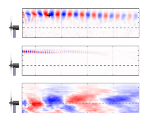
  $\lambda = 5$ in figure 2(b), a number of modes are observed in the accepted Strouhal number range for wake meandering. They are shown in figure 4(g–i) and they again show large-scale coherence. Note that for both the tip speed ratios, the wake meandering mode starts from close to the nacelle and grows radially in the streamwise direction. The wavelength of the mode is shorter near the nacelle and stretches to around $1.5D-2D$ further downstream, which matches well with previous experimental and numerical studies (Howard et al. Reference Howard, Singh, Sotiropoulos and Guala2015; Foti et al. Reference Foti, Yang, Guala and Sotiropoulos2016).

Figure 4. Transverse velocity component of the low-frequency modes (labelled as 1–6 in figure 2) for  $\lambda = 6$ (a–f) and $\lambda = 5$ (g–l).
A number of modes are also observed in the OMD spectra at  $0.4 \lesssim St_D \lesssim 0.5$ and $0.7 \lesssim St_D \lesssim 0.9$. The former when non-dimensionalised by the nacelle's diameter instead of turbine diameter yields a Strouhal number around 0.066–0.083 that is similar to the nacelle's vortex shedding frequency reported in previous studies (Howard et al. Reference Howard, Singh, Sotiropoulos and Guala2015; Abraham et al. Reference Abraham, Dasari and Hong2019). These modes are numbered as modes 3–4 for $\lambda =6$ (figure 2a) and as modes 4–5 for $\lambda =5$ (figure 2b). These modes are however weaker compared with the wake meandering mode and are not spatially as coherent. A potential reason that the nacelle's shedding was not captured well could be due to the fact that the FOV in experiment 1A did not start from immediately downstream of the nacelle's rear face.
Similarly, the modes in the Strouhal number range 0.7–0.9 are most likely related to the shedding from the tower, although the corresponding Strouhal numbers based on the tower's diameter, around 0.074–0.095, are much lower than the expected value of  $\approx$0.2 for vortex shedding behind a two-dimensional circular cylinder at a similar Reynolds number $\approx$4000 based on the tower's diameter (Williamson Reference Williamson1996). Such a reduction in the tower's vortex shedding frequency has been observed earlier (De Cillis et al. Reference De Cillis, Cherubini, Semeraro, Leonardi and De Palma2021; Biswas & Buxton Reference Biswas and Buxton2024). Biswas & Buxton (Reference Biswas and Buxton2024) argued that a number of factors can play a role such as the reduction of the free-stream velocity as the flow passes through the rotor, shear induced on the incoming flow, the unsteadiness in the flow due to the passage of tip and trailing sheet vortices and other three-dimensional effects. As a result, the vortex pattern is significantly distorted from the regular vortex street pattern one might expect. The modes that are expected to be associated with the tower's vortex shedding are shown in figure 4(e,f) for $\lambda =6$ and in figure 4(l) for $\lambda =5$. The modes are much weaker and are not as coherent as the other modes we discussed. This is firstly because of the altered vortex shedding pattern. Secondly, we are only observing the velocity fluctuation parallel to the tower's axis that only arises from the three dimensionality in the vortex shedding pattern and, hence, is not the dominant velocity component associated with the mode.
Unlike experiment 1A, the FOV of experiment 1B included the rear face of the nacelle (see figure 1). Optimal mode decomposition was performed for all the  $\lambda$s obtained from experiment 1B keeping the rank $r$ fixed to 175. The OMD spectra were similar to those obtained from experiment 1A, consisting of the modes related to the tip vortices and an assortment of low-frequency modes ( $St_D<1$). However, the nacelle's shedding mode obtained from experiment 1B was much more coherent than that observed from experiment 1A, as the FOV for the former included part of the nacelle. As an example, the nacelle's shedding mode for $\lambda =5.5$ obtained from experiment 1B is shown in figure 5(a), which shows energetic structures near the nacelle that decay downstream. For a comparison, the wake meandering mode obtained for the same $\lambda$ is shown in figure 5(b), which shows structures of a larger spatial extent that grow downstream and the mode is similar to those observed for experiment 1A.

Figure 5. Transverse velocity components of the OMD modes associated with frequencies (a)  $f_n$ and (b) $f_{wm}$ for $\lambda =5.5$ obtained from experiment 1B.
The OMD modes were also obtained from experiment 2, which considered planes perpendicular to the tower's axis. A selected number of modes are shown in figure 6 for  $\lambda =6$. Figure 6(a–c) shows the modes $f_r - 3f_r$ in the $y=0$ plane that are similar to those observed in figure 3(a–c). In the same plane, figure 6(d) shows the nacelle's shedding mode with a Strouhal number of around 0.069 based on the nacelle's diameter. The tower's shedding mode was not captured in the $y=0$ plane. However, it was captured in the offset plane ( $\kern0.7pt y=-0.35D$) and is shown in figure 6(e). The mode had a Strouhal number of around 0.08 based on the tower's diameter. Note that the mode is much more organised spatially and is more energetic than that observed in the $xy$ plane. Interestingly, no modes could be captured from experiment 2 that resembled the wake meandering modes observed in figure 4. This is probably because the streamwise extent (up to $x/D \approx 1.85D$) of the FOV was not large enough to capture the structures associated with wake meandering that can have wavelengths as large as $1.5D-2D$ (Howard et al. Reference Howard, Singh, Sotiropoulos and Guala2015). Additionally, the wake meandering mode can be expected to be more energetic beyond $x/D \approx 2$ (see figure 5b), making it highly unlikely to be captured in the short FOV.

Figure 6. Transverse velocity components of the OMD modes associated with frequencies (a)  $f_r$, (b) $2f_r$, (c) $3f_r$, (d) $f_n$ obtained in the $xz$
$xz$  $(y=0)$ plane. Subfigure (e) shows the tower's vortex shedding mode at an offset plane $y=-0.35D$. The modes are shown for $\lambda =6$ only.
4. Energy exchanges
The energy exchanges to and from the coherent modes can be explored using the multiscale triple decomposed CKE budget equations developed by Baj & Buxton (Reference Baj and Buxton2017). The CKE budget ( $\tilde {k}_l$) equation can be represented in symbolic form as
 \begin{equation} \frac{\partial \tilde{k}_l}{\partial t} ={-}\tilde{C}_l + \tilde{P}_l - \hat{P}_l +( \tilde{T}^+_l - \tilde{T}^-_l) - \tilde{\epsilon}_l +\tilde{D}_l. \end{equation}
In (4.1) the source terms on the right-hand side consist of convection ( $\tilde {C}_l$), production from the mean flow ( $\tilde {P}_l$), production of stochastic turbulent kinetic energy directly from coherent mode $l$ (
$l$ ( $\hat {P}_l$), triadic energy production ( $\tilde {T}^+_l - \tilde {T}^-_l$), direct dissipation from coherent mode $l$ (
$l$ ( ${\tilde {\epsilon }}_l$) and diffusion ( $\tilde {D}_l$). The full composition of each of these terms is available in Baj & Buxton (Reference Baj and Buxton2017). Baj & Buxton (Reference Baj and Buxton2017) showed that the triadic energy production term can become significant only when there exists three frequencies that linearly combine to zero or, in other words, there is a triad in the form
 \begin{equation} f_l \pm f_m \pm f_n = 0. \end{equation}
Baj & Buxton (Reference Baj and Buxton2017), Biswas et al. (Reference Biswas, Cicolin and Buxton2022) reported the existence of such triads in two different flow configurations involving two-dimensional cylinders of unequal diameters. Note that, for the present case involving a wind turbine wake, the frequencies  $f_r - 6f_r$ form a large number of triads, implying the triadic energy exchange term can play a significant role. We first assess the kinetic energy budgets of the modes obtained from experiment 1A for the tip speed ratios 6 and 5. As we only have planar data, we have to ignore the terms containing out-of-plane velocity and velocity gradients in the energy budget equation. We also have to ignore the contribution to the diffusion term from the pressure. However, as we will show, this simplification does not alter the conclusions of the energy budget analysis. For both $\lambda =6$ and $\lambda =5$, the 12 modes shown in figures 3 and 4 are selected and the stochastic component of the flow is obtained by subtracting these modes from the mean-subtracted velocity field. It is worthwhile mentioning that this process leaves the spectrum of the stochastic turbulence continuous (Baj et al. Reference Baj, Bruce and Buxton2015; Baj & Buxton Reference Baj and Buxton2017).
For an overall understanding, we first integrate the terms from the CKE budget over the entire domain of investigation for all the modes. The results are shown in figure 7(a,b) for  $\lambda =6$ and $\lambda =5$. For the low-frequency modes ( $St_D<1$), including the wake meandering and nacelle or tower's vortex shedding, the primary energy source is the $\tilde {P}_l$ term or energy production from the mean flow, similar to the primary modes discussed in Baj & Buxton (Reference Baj and Buxton2017), Biswas et al. (Reference Biswas, Cicolin and Buxton2022). Among these primary modes, the wake meandering mode draws the highest amount of energy from the mean flow for both $\lambda$s. The wake meandering mode for $\lambda = 6$ is more strongly energised than for $\lambda =5$. A similar dependence of the strength of the wake meandering mode on $\lambda$ was reported in Biswas & Buxton (Reference Biswas and Buxton2024). They established a link between $\lambda$ and the effective porosity of the turbine. As $\lambda$ increased, the effective porosity reduced, resulting in a decrement in the wake meandering frequency and an increment in the strength of the mode. Note from figure 2 that, for the low-frequency modes, multiple triads are possible for which the frequencies sum to $\approx$0. For instance, for $\lambda =6$, $f_1+f_1-f_4 \approx 0$, where $f_1$ is the mode numbered as 1 or the wake meandering mode ( $\,f_{wm}$) and, similarly, $f_4$ is the fourth mode in the spectrum that is believed to be related to the nacelle's shedding ( $\,f_n$). Another possible triad is $f_3+f_4 - f_6 \approx 0$, where $f_3$ and $f_4$ are related to $f_n$ and $f_6$ is likely related to the shedding from the tower ( $\,f_T$). However, the triadic energy production term was not found to be the dominant term for any of these low-frequency modes as can be seen from figure 7. The modes associated with $f_n$ are found to be slightly energised by the $\tilde {T}^+_l - \tilde {T}^-_l$ term, while the wake meandering mode loses some energy due to nonlinear interactions. All the low-frequency modes lose energy primarily through dissipation and production of incoherent (stochastic) turbulence. Hence, we can say that nonlinear triadic interactions are possible among these modes, however, they are not the driving feature of their dynamics.

Figure 7. Energy budget terms of (4.1) summed over the domain of investigation for different modes for (a)  $\lambda =6$ and (b) $\lambda =5$.
The tip vortices on the other hand are energised by a variety of energy sources. For both  $\lambda$s, $f_r$ is primarily energised by the mean flow, thus behaving similarly to a primary mode; $3f_r$ only shows a positive convection ( $-\tilde {C}_l$) term. This is expected as the tip vortices are formed at the passage of the blades and then advected into the PIV domain where they decay monotonically. We can expect a contribution from pressure diffusion to energise the mode, however, this cannot be captured with the current experiments. The nature of $2f_r$ changes with $\lambda$. For $\lambda =6$, it is solely energised by the nonlinear triadic interaction term, hence, it acts like a secondary mode, similar to those observed in two-dimensional multiscale wakes (Baj & Buxton Reference Baj and Buxton2017; Biswas et al. Reference Biswas, Cicolin and Buxton2022). For $\lambda =5$, it is energised primarily by the mean flow production term, while there is also some contribution from the nonlinear triadic interaction term. Therefore, $2f_r$ acts like a ‘mixed mode’ for $\lambda =5$, first reported by Biswas et al. (Reference Biswas, Cicolin and Buxton2022). The modes $4f_r - 6f_r$ are weaker compared with $f_r - 3f_r$. Specifically, $5f_r$ and $6f_r$ for $\lambda =6$ and $4f_r$ and $5f_r$ for $\lambda =5$ exhibited only very weak energy exchanges making it hard to see them in figure 7. Therefore, a ‘ $\boldsymbol {+}$’ or ‘ $\boldsymbol {-}$’ sign is added to represent gain or loss of energy for these modes. A ‘ $\boldsymbol {\sim }$’ sign is shown when the contribution from a term is found to be negligible ( $|\int _x \int _y ED/U_{\infty }^3| <0.01$). Note that, for both $\lambda$s, $6f_r$ behaves similarly to $3f_r$. For $\lambda =6$, $4f_r$ and $5f_r$ behave similarly to $f_r$ and $2f_r$, i.e. like a primary and secondary mode, respectively. For $\lambda =5$ on the other hand, $4f_r$ behaves like $2f_r$ (mixed mode) and $5f_r$ behaves like $f_r$ (primary mode).
For a deeper understanding of the energy budget terms, we take a spanwise (along the  $y$ direction) integral of the budget terms and look at their streamwise variation. This is first shown for the modes $f_r - 3f_r$ for the two $\lambda$s in figure 8. The corresponding plots for $4f_r - 6f_r$ are not shown as their budgets were similar to one of the first three modes ( $\,f_r - 3f_r$) as discussed earlier. Note that we consider the budgets in a time-averaged sense so ${\rm d}k/{\rm d}t$ is essentially zero; therefore, the combined effect of the various terms of the CKE budget equation is reflected in the convection term ( $-\tilde {C}_l$): if the energy content of the mode is increasing with downstream distance (it is being net energised) then this term will be negative whilst it will be positive when the mode is spatially decaying.

Figure 8. Streamwise evolution of the spanwise-averaged (along  $y$) energy budget terms of (4.1) for (a) $f_r$, (b) $2f_r$ and (c) $3f_r$ for $\lambda =6$. Subfigures (d–f) show the same for $\lambda =5$.
For  $f_r$ (figure 8a,d), the primary source is the $\tilde {P}_l$ term, shown with a black line. Note that, for $\lambda =6$, the $\tilde {P}_l$ term changes sign at $x/D \approx 1.65$. This location is close to where $f_r$ was found to be the most energetic (see figure 3a). Beyond this point the mode decays monotonically as indicated by the convection ( $-\tilde {C}_l$) term being positive. For brevity, let us denote the location where $\tilde {P}_l$ changes sign as $x_{wr}$. Note that $x_{wr}$ is particularly important in terms of wake recovery, as beyond this point the mode transfers energy back to the mean flow. For $\lambda =5$ (figure 8d), $x_{wr} \approx 3.2$ that implies that wake recovery starts much later. Note that, for $\lambda =5$, there is a drop in the $\tilde {P}_l$ term of $f_r$ at $x/D \approx 1$. This is because of the presence of the merged root vortices (with frequency $f_r$) that decay in this region and noting that the $\tilde {P}_l$ term is essentially the sum of contributions from both the root and tip regions.
For  $\lambda =6$, $2f_r$ is primarily energised by the triadic interaction term that drops off to zero at $x/D \approx 1.6$; this is again close to the point where $2f_r$ is most energetic in figure 3(b). From figure 3 we can see that, for $\lambda =5$, $2f_r$ is much weaker than for $\lambda =6$. This is corroborated by the fact that the magnitude of the energy budget terms of $2f_r$ in figure 8 is smaller for $\lambda =5$, compared with $\lambda =6$. Additionally, for the lower $\lambda$, the triadic interaction term is much weaker due to increased separation between the tip vortices. Therefore, unlike $\lambda =6$, for $\lambda =5$, $2f_r$ is energised mainly by the mean flow. For $3f_r$, the convection term is positive throughout as it decays monotonically in the domain. The trends are qualitatively similar for both the $\lambda$s. Note also that the residuals of the budget equation are highest for $3f_r$, especially closer to the rotor. This is probably because there is a significant role of the pressure diffusion term in this region that has been neglected in the analysis.
The same analysis is performed with the data from experiment 2A (see table 1 for details) that considered the orthogonal  $xz$ plane for $\lambda =6$. The budget terms are summed in the $z$ direction and are shown in figure 9 for the modes $f_r - 3f_r$. Note that the trends of the budget terms are quite similar to those observed in the $xy$ plane earlier (in figure 8). The dominant source terms of the modes are the same. Moreover, the $\tilde {P}_l$ term for $f_r$ changes sign at the same location as before, at $x/D \approx 1.65$. Similarly, the triadic interaction term for $2f_r$ changes sign at $x/D \approx 1.6$, consistent with the observation in the $xy$ plane. This similarity of the budget terms in the two orthogonal planes shows that the budget terms are close to axisymmetric in nature and offers reassurance as to the repeatability of our results.

Figure 9. Streamwise evolution of the energy budget terms of (4.1) averaged along the  $z$ direction for (a) $f_r$, (b) $2f_r$ and (c) $3f_r$ for $\lambda =6$.
Figure 10 shows the evolution of the CKE budget terms for selected low-frequency modes in different PIV planes for  $\lambda =6$. Figure 10(a) shows the terms for the dominant wake meandering mode obtained from experiment 1A (the mode shown in figure 4a). Figure 10(b,c) shows the same for the nacelle's and the tower's shedding mode obtained from experiments 2A and 2B, respectively. The terms appear to be noisier compared with the tip vortex system; however, the $\tilde {P}_l$ term is unambiguously the dominant source term for these modes. For the wake meandering mode, $\tilde {P}_l$ slowly grows with streamwise distance, which is consistent with the observed far-wake dominance of wake meandering (Biswas & Buxton Reference Biswas and Buxton2024). The sheddings from the nacelle and the tower on the other hand quickly drop to zero, showing their relatively transient spatial nature.

Figure 10. Streamwise evolution of the spanwise-averaged (along  $y$) energy budget terms of (4.1) for (a) $f_{wm}$ in the $xy$ plane. Streamwise evolution of the energy budget terms averaged along the $z$ direction for (b) $f_n$ in the $y=0$ plane, (c) $f_T$ in the $y=-0.35D$ plane.
4.1. Triadic interactions
Let us now cast a closer look at the triadic energy exchange term. So far we only know that for  $\lambda =6$, $2f_r$ is energised primarily by the triadic energy exchange term. But, $2f_r$ forms a number of triads and the triadic energy gain of $2f_r$ is a sum of contributions from all the triads that $2f_r$ can form with the other frequencies. At this point we can ask are there any particular triads that are more important or are there any frequencies that transfer more energy to $2f_r$? Answering these questions can help significantly simplify what would be a rather complicated network of energy transfers in the tip vortex system. The terms $\tilde {T}^+_l$ and $\tilde {T}^-_l$ in (4.1) indicate the net nonlinear energy gain and loss, respectively, from the $l_{th}$ coherent mode and are defined as follows:
 \begin{equation}
\tilde{T}^+_{l} ={-}\frac{1}{2}\sum_{f_s,f_t}\overline{\tilde{u}^{\,f_l}_i
\tilde{u}^{\,f_t}_j \frac{\partial
\tilde{u}^{\,f_s}_i}{\partial x_j}}, \quad \tilde{T}^-_{l}
={-}\frac{1}{2}\sum_{\,f_s,f_t}\overline{\tilde{u}^{\,f_s}_i
\tilde{u}^{\,f_t}_j \frac{\partial
\tilde{u}^{\,f_l}_i}{\partial x_j}}.
\end{equation}
\begin{equation}
\tilde{T}^+_{l} ={-}\frac{1}{2}\sum_{f_s,f_t}\overline{\tilde{u}^{\,f_l}_i
\tilde{u}^{\,f_t}_j \frac{\partial
\tilde{u}^{\,f_s}_i}{\partial x_j}}, \quad \tilde{T}^-_{l}
={-}\frac{1}{2}\sum_{\,f_s,f_t}\overline{\tilde{u}^{\,f_s}_i
\tilde{u}^{\,f_t}_j \frac{\partial
\tilde{u}^{\,f_l}_i}{\partial x_j}}.
\end{equation}
Note that the terms consist of three frequencies and are non-negligible only when the frequencies form a triad (Baj & Buxton Reference Baj and Buxton2017). Essentially we take contributions from all possible triads by summing over the two frequencies ( $\,f_s$ and $f_t$). Instead, we can fix one of these two frequencies (let us say $f_s$) and can take a summation over the other frequency ( $\,f_t$). This would give us the net triadic energy exchange between $f_l$ and $f_s$. We do this for all the frequencies related to the tip vortices ( $\,f_r - 6f_r$) and show the results in figure 11 for the two $\lambda$s. The arrows show the direction of energy transfer. For instance, the first row shows the net amount of energy $f_r$ is giving away to the other frequencies. In other words, the first column shows the amount of energy received by $f_r$ from all other frequencies. As observed earlier, the magnitude of the traidic energy transfers are much stronger for $\lambda =6$, compared with $\lambda =5$. Moreover, for $\lambda =6$, most of the energy transfer is limited between $f_r - 4f_r$, while the contributions from $5f_r$ and $6f_r$ are significantly weaker in comparison. Looking at the second column in figure 11(a) we can say that the main source for $2f_r$'s triadic energy gain is $3f_r$. Thereafter, $2f_r$ transfers some amount of energy to $f_r$, hence forming a net inverse energy cascade. Note that this sequence of energy transfer is similar to that predicted by Felli et al. (Reference Felli, Camussi and Di Felice2011) (see figure 41b of Felli et al. Reference Felli, Camussi and Di Felice2011) for a three-bladed turbine. However, the fact that the higher harmonics can also have an important role in the energy exchange process was not highlighted in their work. Note from figure 11(a) that $f_r$ transfers a significant amount of energy to $4f_r$ and $4f_r$ transfers almost the same amount of energy to $3f_r$. Therefore, although $4f_r$ does not gain energy through triadic interactions, it forms a bypass route of energy transfer allowing $f_r$ to transfer some energy back to $3f_r$.

Figure 11. Triadic energy exchanges for (a)  $\lambda =6$ and (b) $\lambda =5$ from experiment 1A.
For  $\lambda =5$, figure 11(b) shows that not only are the magnitudes of the energy transfers weaker but the energy transfer pathways are also different. This includes the fact that the net nonlinear energy gain for $2f_r$ is now quite small, as was previously shown in figure 7(b). Unlike for $\lambda =6$, $2f_r$ and $4f_r$ are both energised mainly by $f_r$, as far as triadic interaction is concerned. To further understand the dependence of these energy transfers on $\lambda$, the analysis is repeated for other $\lambda$s in experiment 1B. These are shown in figure 12 in combination with the results for $\lambda =6$ and $\lambda =5$ (from experiment 1A) for a better comparison. Note that the extents of the FOV are different for experiment 1B. Therefore, in order to be consistent across different FOV sizes, the triadic energy exchanges are integrated between $0.5 < x/D <3D$ and $0< y/D<0.75D$. Note that as we increase $\lambda$ from 5 to 6, there is a clear transition in the energy exchange pathway. For $\lambda =5.5$, the pattern looks exactly similar to that for $\lambda =6$. For $\lambda =5.3$, the pattern appears to be at an intermediate state between that for $\lambda =5$ and $\lambda =5.5$. From $\lambda =5.5$, the energy exchange pattern remains qualitatively similar as we increase $\lambda$ and the magnitude of the energy transfers increases showing a stronger nonlinear interaction between the modes at higher $\lambda$.

Figure 12. Net traidic transfers for (a)  $\lambda = 5$, (b) $\lambda = 5.3$, (c) $\lambda = 5.5$, (d) $\lambda = 6$, (e) $\lambda = 6.6$, ( f) $\lambda = 6.9$.
From figure 11(a) we can see that, for  $\lambda =6$, $2f_r$ gets most of its energy from $3f_r$. However, $2f_r$ and $3f_r$ can form two triads together, one with $f_r$ and another with $5f_r$, hence, it is not clearly known which triad is more important. We thus further split the inter-frequency energy transfers shown in figure 11 into contributions from different triads. For brevity, we present the results only for $\lambda =6$ as it showed stronger nonlinear interactions. In figure 13 we show the streamwise evolution of the spanwise-averaged inter-frequency energy transfers that correspond to different triads. Note that there are a total of nine triads involving the frequencies $f_r - 6f_r$. These are shown in boxes of different colours and line types in figure 13 for an easier interpretation. The first six triads involve three different frequencies and are shown in boxes with a solid line, let us call them triad type $I$. The last three triads have a repeated frequency and are shown in boxes with a dash-dotted line to distinguish them. These triads are termed triad type $II$. We first show the energy transfers to $f_r$ from the other frequencies in different triads in figure 13(a). Note that $f_r$ forms four triads of type $I$ and one triad of type $II$. For each triad of type $I$, it is possible to have two energy transfers to $f_r$ from the other two frequencies involved in the triad. For triads of type $II$, there will be only one transfer. Accordingly, we have a total of nine transfers to $f_r$ as indicated in figure 13(a). The transfers corresponding to the first triad (shown in the blue solid box) are shown with blue lines. The transfer from the lower of the two frequencies of the triad (i.e. $2f_r$) is shown in a solid blue line and that from the higher frequency ( $3f_r$) is shown in a dashed blue line. The transfer from the seventh triad (shown in a black dash-dotted box) is shown in a black dash-dotted line. This same convention is used throughout to avoid confusion. Note that, for $f_r$, only three triads 1, 2 and 7 are important. For $2f_r$, only triads 1 and 7 are found to be important and both positively energise $2f_r$. The main source of energy for $2f_r$ is however $3f_r$ from triad 1 as discussed earlier. For $3f_r$, only triads 1 and 2 are important. As a whole, $3f_r$ loses energy, most of which goes to energise $2f_r$. For $4f_r$, only the second triad is important. The energy transfers involving $5f_r$ and $6f_r$ are an order of magnitude smaller and can be ignored.

Figure 13. Energy transfers from different frequencies in different triads to (a)  $f_r$, (b) $2f_r$, (c) $3f_r$, (d) $4f_r$, (e) $5f_r$ and ( f) $6f_r$. The possible traids are shown on the right.
5. Summary of the energy exchanges for the tip vortices
The analysis of § 4 allows us to drastically simplify the network of nonlinear energy exchanges by using a fewer number of triads. To be specific, for  $\lambda =6$, we can only retain triads 1, 2 and 7 (shown in figure 13) and discard the rest. This approximated network of energy transfers is schematically shown in figure 14(a) and it summarises the key energy exchanges in the tip vortex system discussed above. The energy exchanges in triads 1 and 2 are shown in blue and red solid lines, respectively, while the black dash-dotted line represents the energy transfer in triad 7, similar to the convention used in figure 13. The values show the net triadic energy transfers. Note that triads 1 and 2 show a cyclic nature of energy transfers and form a net inverse energy cascade (i.e. energy transfer from high to low frequency), while triad 7 shows a forward cascade. For a comparison, the positive contributions from the mean flow production term ( $\tilde {P}_l$) in (4.1) are also shown by solid black lines. The numbers show the magnitudes of the energy transfers and the same is also highlighted by the thicknesses of the arrows.

Figure 14. Triadic energy transfer pathways among the modes  $f_r - 4f_r$ for (a) $\lambda =6$ and (c) $\lambda =5$. The line types and the colour of the arrows showing inter-frequency energy transfers are consistent with those used to represent triads in figure 13. The solid black arrow shows the positive contribution from the $\tilde {P}_l$ term in (4.1). The thickness of the arrows varies according to the magnitude of the energy transfers as indicated. Panel (b) shows the magnitudes of the energy transfers from $3f_r$ to $2f_r$ in triad 1 and from $4f_r$ to $3f_r$ in triad 2 for different $\lambda$s.
To summarise the energy transfer process involving the tip vortices, we can say from triad 1 that energy primarily flows from  $3f_r$ towards $f_r$ via the secondary mode $2f_r$, which is a nice representation of the tip vortex merging process (Felli et al. Reference Felli, Camussi and Di Felice2011). However, we interestingly find that the net triadic energy gain of $f_r$ is nearly zero. This is because $f_r$ transfers most of its triadic energy gain to $4f_r$. Therefore, $f_r$ is primarily sustained by energy supply from the mean flow leading us to term it as a primary mode. Similarly, $4f_r$ also behaves like a primary mode, transferring the energy it gains from $f_r$ to $3f_r$. This energy feedback slows down the energy drainage of $3f_r$. We therefore argue that the energy transfers from $3f_r$ to $2f_r$ in triad 1 and from $4f_r$ to $3f_r$ in triad 2 can be linked to the stability and sustainment of the tip vortices. We compare these two energy transfers for the four $\lambda$s (5.5, 6, 6.6, 6.9) that showed similar triadic energy exchange patterns (figure 12) in figure 14(b). Note that both the energy transfers increase with $\lambda$. However, the difference of the two energy transfers also increases with $\lambda$, indicating a faster decay of the tip vortices at a higher $\lambda$.
A similar schematic of energy transfers among the modes  $f_r - 4f_r$ for $\lambda =5$ is shown in figure 14(c). Note that, for $\lambda =5$, a simplification of the energy transfer network is not readily possible as all the modes exhibit energy transfers of similar magnitudes to/from them (see figure 11b). Therefore, the purpose of figure 14(c) is solely to compare triads 1, 2 and 7 between $\lambda =5$ and $\lambda =6$. First of all, the energy transfers are much weaker for $\lambda =5$. Secondly, although triad 2 is still cyclic in nature, triad 1 has become non-cyclic. The primary change has occurred around $2f_r$ that is no longer strongly energised by $3f_r$. Triads 1 and 7 contribute to some nonlinear energy gain of $2f_r$ but it gets most of its energy from the mean flow.
These energy exchanges can elucidate the nature of the tip vortex merging process. Recently, Biswas & Buxton (Reference Biswas and Buxton2024) reported two different merging processes for two different  $\lambda$s using the same wind turbine model. For the lower $\lambda$ ( $\lambda =4.5$), the merging of the tip vortices resembled a two-step process where first $2f_r$ was formed and $f_r$ became energetic further downstream, as also reported by Felli et al. (Reference Felli, Camussi and Di Felice2011) and Sherry et al. (Reference Sherry, Nemes, Lo Jacono, Blackburn and Sheridan2013). Contrastingly, for the higher $\lambda$ ( $\lambda =6$), three tip vortices appeared to combine almost directly in what they referred to as a one-step process (see also supplementary video 2 of Biswas & Buxton Reference Biswas and Buxton2024). For the same $\lambda$, we however do not see a direct energy transfer from $3f_r$ to $f_r$ in figure 14(a), as one might expect from a one-step process. The energy transfer still happens in two steps, first from $3f_r$ to $2f_r$ and then from $2f_r$ to $f_r$ as predicted by Felli et al. (Reference Felli, Camussi and Di Felice2011). However, due to the fact that $f_r$ and $2f_r$ attain their maximum energy at almost the same streamwise location (see figure 3a,b), we can say that these two steps take place almost concurrently, making it look like a one-step process. For $\lambda =5$, there is a larger streamwise separation between the points where $f_r$ and $2f_r$ attain their maximum energy, visually indicating a two-step merging process. The increased separation between the helices at the lower $\lambda$, however, results in a much weaker nonlinear interaction. Furthermore, the injection of energy from the mean flow to $2f_r$ results in a reorganisation of the energy transfer pattern in triad 1, i.e. from a cyclic to a non-cyclic one.
It is worthwhile mentioning that the energy budget terms for the tip vortices may be a function of the chord-based Reynolds number ( $Re_c$). At a lower $Re_c$, the larger viscous effects result in a higher drag and limits the maximum lift coefficient (Lissaman Reference Lissaman1983). Therefore, since utility-scale wind turbines operate at a much higher $Re_c$, the blade sections experience a higher $C_l$ and lower $C_d$. Since $C_l$ is directly related to the bound circulation, we can expect the strength of the tip vortices (shed circulation) to increase with $Re_c$. The stronger tip vortices result in an interaction that occurs earlier (further upstream) that can in turn be linked to the observed faster wake expansion and wake recovery at higher Reynolds numbers (McTavish et al. Reference McTavish, Feszty and Nitzsche2013; Bourhis et al. Reference Bourhis, Pereira and Ravelet2023). Therefore, we believe increasing $Re_c$ would further increase the magnitudes of the nonlinear triadic energy exchanges for the tip vortices at a given $\lambda$. It will be interesting to study and compare the separate effects of increasing $Re_c$ and $\lambda$ on the triadic interactions and the tip vortex merging process. From the nature of the Biot–Savart law, which governs the interaction between the tip vortices, we can vaguely expect the growth of the tip vortex instability to be directly proportional to the strength of the vortices, and inversely proportional to the square of the separation (Sørensen et al. Reference Sørensen, Mikkelsen, Henningson, Ivanell, Sarmast and Andersen2015). Now, increasing $\lambda$ results in a reduction of the separation (pitch of the helices) and can increase the strength of the tip vortices, while increasing $Re$ is expected to only increase the strength of the tip vortices. Further, the recent study by Biswas & Buxton (Reference Biswas and Buxton2024) compared the tip vortex merging process at a low and high $\lambda$ and reported that the stronger interaction at the higher $\lambda$ was primarily driven by the reduced separation. To summarise, we can say that the tip vortex merging process likely depends on $Re_c$, however, it is more likely a stronger function of $\lambda$.
6. The near wake and wake recovery
For a wind turbine, it is important to quantify the extent of the near wake, particularly in the context of designing wind farm layouts as the near wake contains energetic coherent structures capable of inducing fatigue damage to the subsequent turbines. The extent of the near wake depends on several factors such as the nature and intensity of the free-stream turbulence level, turbine geometry, operating condition and so on and, hence, it is often vaguely defined between 2–4 rotor diameters downstream of the rotor (Vermeer, Sørensen & Crespo Reference Vermeer, Sørensen and Crespo2003; Foti et al. Reference Foti, Yang, Guala and Sotiropoulos2016). Several attempts have been made to quantify the near wake, for instance, by observing self-similarity in the time-averaged wake profile (Sørensen et al. Reference Sørensen, Mikkelsen, Henningson, Ivanell, Sarmast and Andersen2015) or by looking at the variation of time-averaged coherent or turbulent kinetic energy in the wake (De Cillis et al. Reference De Cillis, Cherubini, Semeraro, Leonardi and De Palma2021; Gambuzza & Ganapathisubramani Reference Gambuzza and Ganapathisubramani2023). In contrast, Biswas & Buxton (Reference Biswas and Buxton2024) endorsed a more dynamic point of view and defined the extent of the near wake as the location where the strength of wake meandering or  $f_{wm}$ (dominant dynamic feature in the far wake) surpassed that of the tip vortices or $3f_r$ (dominant frequency in the near wake). They also defined a convective length scale, $L_c = {\rm \pi}D/\lambda$ (which can be physically interpreted as the distance travelled at the free-stream velocity in the time taken for one complete rotation of the turbine), and reported that the near wake location was ${\approx } 3L_c$ for a range of $\lambda$s tested, or in other words, the near wake's extent scaled with $1/\lambda$. The strength of a frequency at a particular streamwise ( $x$) location was however defined as the magnitude of the spectral peak at that particular frequency. As the strengths of the frequencies depended only on $x$, the spatial distribution of the strength or energy associated with frequencies was not taken into account in the definition of the near wake. In this section we explore other ways to quantify the extents of the near/far wake based on the knowledge gained earlier about the nature of the different modes and the energy exchanges to/from them.
We first obtain the time-averaged kinetic energy of the modes associated with  $f_{wm}$ ( $k_{f_{wm}}$) and $f_r$ ( $k_{f_r}$) and plot the relative kinetic energy $k_{f_{wm}} - k_{f_r}$ for $\lambda = 6$ and $\lambda =5$ in figures 15(a) and 15(b), respectively. The solid black line corresponding to $k_{f_{wm}} - k_{f_r} = 0$ nicely distinguishes the regions where $f_{wm}$ or $f_r$ is stronger than the other. Similarly, the dashed black line shows the contour corresponding to $k_{f_{wm}} - k_{3f_r} = 0$ that is always found to be located within the contour traced by $k_{f_{wm}} - k_{f_r} = 0$ for the $\lambda$s tested. Similar contours can be obtained using the harmonics of $f_r$ and $3f_r$, but they are generally weaker in nature. We therefore propose that $k_{f_{wm}} - k_{f_r} = 0$ can be used to distinguish the inner wake involving low-frequency dynamics from the outer wake that contains high-frequency modes related to the tip vortices. The earlier and stronger tip vortex merging process for $\lambda =6$ results in a quicker disintegration of the tip vortex system. The outer wake thus vanishes at $x/D \approx 4.7$, creating a path for rapid exchange of mass and momentum between the inner wake and the non-turbulent background fluid in this case, aiding wake recovery. We therefore argue that the end of the outer wake can be considered as the initiation of the far wake where wake meandering is the only discernible frequency signature. The extent of the outer wake and, hence, the far wake depends on $\lambda$. For $\lambda =5$, the outer wake extends beyond $x/D =5$; therefore, we can expect the far wake to also scale with $1/\lambda$ at least in the presence of low inflow turbulence, similar to the near wake (Biswas & Buxton Reference Biswas and Buxton2024).

Figure 15. Filled contours showing relative kinetic energy of the wake meandering mode with respect to the mode associated with  $f_r$ (denoted by $\tilde {k}_{f_{wm}} - \tilde {k}_{f_r}$) for (a) $\lambda =6$ and (b) $\lambda =5$. The solid and dashed black lines correspond to $\tilde {k}_{f_{wm}} - \tilde {k}_{f_r}=0$ and $\tilde {k}_{f_{wm}} - \tilde {k}_{3f_r}=0$, respectively. The $\boldsymbol {+}$ sign shows the location where the kinetic energy corresponding to $f_r$ is maximum. The dash-dotted vertical line shows the streamwise location corresponding to 3 convective length scales or $3L_c$ defined in Biswas & Buxton (Reference Biswas and Buxton2024).
Next we look at the evolution of the mean flow production term ( $\tilde {P}_l$) of the tip vortex system. In figure 16(a) we show the streamwise evolution of the spanwise-averaged (along $y$) mean flow production term for the tip vortex system ( $\sum _{l=f_r}^{l=6f_r} \tilde {P}_l$) for three different $\lambda$s (represented by solid lines). While the dashed lines show the mean flow production term only for $f_r$ ( $\tilde {P}_{f_r}$) for the corresponding $\lambda$s. Note that $\tilde {P}_{f_r}$ is close to $\sum _{l=f_r}^{l=6f_r} \tilde {P}_l$ for all $\lambda$s, which implies that most of the energy exchanges between the mean flow and the tip vortex system happens through $f_r$. As discussed earlier, disintegration of the tip vortex system is essential to re-energise the wake. Note that close to the rotor $\sum _{l=f_r}^{l=6f_r} \tilde {P}_l > 0$, i.e. the tip vortex system first draws energy from the mean flow as a whole. However, after some distance downstream it starts to transfer the energy back to the mean flow as indicated by $\sum _{l=f_r}^{l=6f_r} \tilde {P}_l <0$. The streamwise location where the combined mean flow production term for the tip vortex system changes sign can be ascribed as the point of initiation of wake recovery (let us denote it by $x_{wr}$). Note that, as $\lambda$ increases, $x_{wr}$ moves closer to the turbine. Moreover, an estimation of $x_{wr}$ can be obtained just by looking at the production term of $f_r$ that again highlights the importance of $f_r$ in the distinction of the near wake from the far wake. In figure 16(b) we show the variation of $x_{wr}$ obtained from $\tilde {P}_{f_r}$ with $\lambda$. The extent of the near wake, ${\approx } 3L_c$, proposed by Biswas & Buxton (Reference Biswas and Buxton2024) is also shown for a comparison. Here $x_{wr}$ shows a nice trend with $\lambda$. More interestingly, for higher $\lambda$, $x_{wr}$ becomes close to $3L_c$, further highlighting the efficacy of $L_c$ as a length scale in the near wake.

Figure 16. (a) Streamwise variation of spanwise-averaged mean flow production term for the tip vortex system (shown by the solid lines) and  $f_r$ (shown by the dashed line) for different $\lambda$s. (b) The variation of the location where wake recovery initiates or $x_{wr}$ with $\lambda$ (blue, – $\bullet$–). The solid black line shows the streamwise location $x/D = 3L_c$.
To understand why the  $\tilde {P}_l$ term for $f_r$ changes sign after some distance downstream, let us take a closer look at its composition. Baj & Buxton (Reference Baj and Buxton2017) defined the term as $\tilde {P}_l = -\sum _m \overline {\tilde {u}^m_i \tilde {u}^l_j} ({\partial \overline {u}_i}/{\partial x_j})$, where $m$ can be any coherent mode selected in the reduced-order representation of the flow including the $l_{th}$ mode. Assuming that the velocity components of the different modes are uncorrelated, i.e. $\overline {\tilde {u}^l_i \tilde {u}^m_j} \approx 0$ for any $l \neq m$, we can say that $\tilde {P}_l \approx -\overline {\tilde {u}^l_i \tilde {u}^l_j} ({\partial \overline {u}_i}/{\partial x_j})$. Next, we can show that the transverse gradient of the streamwise velocity ( ${\partial \bar {u}}/{\partial y}$) is an order of magnitude stronger than the other gradients, at least in the tip shear layer region. So we can further approximate the term as $\tilde {P}_l \approx -\overline {\tilde {u}^l \tilde {v}^l} ({\partial \bar {u}}/{\partial y})$. In figure 17(a) we show the $\tilde {P}_l$ (without any approximation) field for $f_r$. As can be expected, $\tilde {P}_l$ is concentrated only in the tip shear layer region and the ‘ $\boldsymbol {+}$’ sign shows the location where the term changes sign, i.e. the location of the onset of wake recovery ( $x_{wr}$). Figure 17(b) shows the $\tilde {P}_l$ field only with the dominant term ( $-\overline {\tilde {u}^l \tilde {v}^l} ({\partial \bar {u}}/{\partial y})$) and it looks almost exactly similar to figure 17(a), hence justifying the approximation.

Figure 17. (a) Mean flow production term ( $\tilde {P}_l$) of $f_r$ for $\lambda =6$, (b) shows the leading term of $\tilde {P}_l$. The ‘ $\boldsymbol {+}$’ sign marks the location of the sign change.
Now,  ${\partial \bar {u}}/{\partial y}$ is always positive in the tip shear layer region. The observed change of sign in $\tilde {P}_l$ thus requires a change in the nature of correlation (negative to positive) between the streamwise and transverse velocity components of $f_r$. This is similar to the observation of Lignarolo et al. (Reference Lignarolo, Ragni, Scarano, Ferreira and Van Bussel2015) for a two-bladed turbine. They argued that the net transport of kinetic energy towards the wake centreline (the component contributing to the wake recovery) due to the periodic motions can be given by the gradients of the kinetic energy flux $-\overline {\tilde {u}^l \tilde {v}^l}\bar {u}$. They further showed that at a certain distance downstream, the orientation/inclination of the tip vortex pair undergoing merging with respect to the streamwise direction changed from negative ( ${<}90^\circ$) to positive ( ${>}90^\circ$), resulting in a change in the correlation between the streamwise and transverse velocity component (see figure 17 of Lignarolo et al. Reference Lignarolo, Ragni, Scarano, Ferreira and Van Bussel2015). From figure 1 here and also from supplementary video 2 of Biswas & Buxton (Reference Biswas and Buxton2024), we can see that for $\lambda =6$, the vortex triplet, undergoing merger, changes its inclination at $x/D \approx 1.5$. Consequently, we observe a sign change in the $\tilde {P}_l$ term for $f_r$ at $x/D \approx 1.5$ for $\lambda =6$.
7. Conclusion
The near wake of a wind turbine is abundant with coherent structures. Studying the interaction between these coherent structures is a key to understanding the spatio-temporal evolution of the wake and phenomena like wake recovery. We conducted PIV experiments to identify and extract the coherent structures in the near wake of a rotor model having a nacelle and a tower, thereby making it representative of a utility-scale wind turbine for two main tip speed ratios ( $\lambda$), $\lambda =6$ and $\lambda =5$. The coherent structures were identified using a multiscale triple decomposition of the velocity field using OMD (Wynn et al. Reference Wynn, Pearson, Ganapathisubramani and Goulart2013; Baj et al. Reference Baj, Bruce and Buxton2015). A large number of high-frequency modes were extracted related to the tip vortices, including modes with a frequency equal to the turbine's rotational frequency ( $\,f_r$), blade passing frequency ( $3f_r$) and their harmonics ( $2f_r$ and $4f_r - 6f_r$ ) as well as a number of low-frequency modes that included sheddings from the tower ( $\,f_T$), the nacelle ( $\,f_n$) and wake meandering ( $\,f_{wm}$). The spatial nature and strength of the modes depended on $\lambda$. For the higher $\lambda$ ( $\lambda =6$), the modes related to the tip vortices were energetic closer to the rotor, owing to the early interaction between the tip vortices for a higher $\lambda$ (Sherry et al. Reference Sherry, Nemes, Lo Jacono, Blackburn and Sheridan2013). For the low-frequency modes, the modes associated with $f_n$ and $f_T$ were similar for the two $\lambda$s. Interestingly however, the wake meandering mode was found to be more energetic for the higher $\lambda$ consistent with the observations of Biswas & Buxton (Reference Biswas and Buxton2024).
Further insights are gained about the nature of the different modes by studying the energy exchanges to and from them by using the multiscale triple decomposed CKE budget equation derived by Baj & Buxton (Reference Baj and Buxton2017). The low-frequency modes associated with the sheddings from the tower and the nacelle as well as the wake meandering mode were found to be primarily energised by the mean flow, hence acting similarly to a ‘primary mode’, as termed in previous studies (Baj & Buxton Reference Baj and Buxton2017; Biswas et al. Reference Biswas, Cicolin and Buxton2022). The tip vortex system on the other hand was found to have a variety of energy sources such as energy production from the mean flow, nonlinear triadic energy production or both. The mode associated with  $f_r$ behaved like a primary mode for both $\lambda$s, while the nature of $2f_r$ changed with $\lambda$. For $\lambda =6$, $2f_r$ gained most of its energy through the nonlinear triadic energy production term in the CKE budget equation, hence, it is akin to a ‘secondary mode’ (Baj & Buxton Reference Baj and Buxton2017; Biswas et al. Reference Biswas, Cicolin and Buxton2022). For $\lambda =5$ on the other hand, the mode received most of its energy through the mean flow production term, while having a non-negligible positive contribution from the triadic interaction term, therefore acting like a ‘mixed mode’ as discussed in Biswas et al. (Reference Biswas, Cicolin and Buxton2022). The differences in the energy exchanges observed for the higher and lower $\lambda$ were shown to be consistent with the ‘one-step’ and ‘two-step’ merging processes reported earlier by Biswas & Buxton (Reference Biswas and Buxton2024). Some triadic interaction was observed between the low-frequency modes as well, but its net contribution was small compared with the energy production from the mean flow.
A complex network of triadic energy exchanges between the modes associated with  $f_r - 6f_r$ is identified and discussed. For $\lambda =6$, energy was found to flow from $3f_r$ to $2f_r$ and then from $2f_r$ to $f_r$ via the nonlinear triadic interaction term in the triad formed by $f_r, 2f_r$ and $3f_r$, similar to the observation of Felli et al. (Reference Felli, Camussi and Di Felice2011). In the triad formed by $f_r, 3f_r$ and $4f_r$, $f_r$ transferred some energy to $4f_r$. Mode $4f_r$ then transferred almost the same amount of energy to $3f_r$, resulting in a much weaker but still dynamically important $4f_r$ mode. The same pattern of triadic energy exchanges was observed for four different $\lambda$s ( $\lambda =5.5$, $\lambda =6$, $\lambda =6.6$ and $\lambda =6.9$). The triadic energy exchanges for the lower $\lambda$s were found to be much weaker due to the increased separation between the tip vortex filaments.
Finally, attempts are made to identify the boundaries between the inner/outer wake and near/far wake based on the modes and their energy contents. It is shown that the inner wake (involving low-frequency dynamics) can be distinguished from the outer wake (involving high-frequency structures) by comparing the kinetic energy associated with the turbine's rotational frequency  $f_r$ and wake meandering ( $\,f_{wm}$). To identify the location of the onset of wake recovery (defined as $x_{wr}$), we looked at the combined mean flow production term of the modes related to the tip vortices ( $\,f_r - 6f_r$). Initially, the tip vortex system was found to extract energy from the mean flow, but further downstream, the combined production term became negative, implying a net energy transfer back to the mean flow. More interestingly, most of the energy exchange between the mean flow and the tip vortex system was found to happen through the turbine's rotational frequency. The sign change in the mean flow production term of $f_r$ was shown to be related to a switch in the nature of correlation between the streamwise and transverse velocity components of the $f_r$ mode resulting from the change of inclination of the tip vortex system undergoing merging, similar to the observation of Lignarolo et al. (Reference Lignarolo, Ragni, Scarano, Ferreira and Van Bussel2015) for a two-bladed rotor.
Funding
N.B. gratefully acknowledges funding through the Imperial College London President's Scholarship and the Engineering and Physical Sciences Research Council (EPSRC) through grant EP/T51780X/1. O.B. gratefully acknowledges funding from EPSRC through grant no. EP/V006436/1.
Declaration of interests
The authors report no conflict of interest. For the purposes of open access, the authors have applied a Creative Commons Attribution (CC BY) licence to any Author Accepted Manuscript (AAM) version arising.
Appendix A. Convergence of the OMD modes
To estimate the possible effects of the rank  $r$ of the OMD matrices (which needs to be selected a priori), the decomposition is performed with different $r$s. Optimal mode decomposition is first applied to the data set from experiment 1A for $\lambda =6$ for different $r$s. The resultant spectra are shown in figure 18(a). For $r=125$, only the modes from $f_r - 3f_r$ are captured. While, for the higher ranks, $4f_r$ is also captured. The dominant wake meandering frequency around $St_D\approx 0.2$ was captured for all the $r$s as well as frequencies in the range $0.4\lesssim St_D \lesssim 0.5$ and $0.7\lesssim St_D \lesssim 0.9$ that are associated with the vortex sheddings from the nacelle and the tower, respectively. To evaluate the effect of $r$ on the energy budget analysis, we look at the primary source term for $f_r$ and $f_{wm}$, i.e. the coherent energy production term ( $\tilde {P}_l$) for different $r$s. The streamwise evolution of the spanwise-averaged $\tilde {P}_l$ term for the frequencies are shown in figure 18(b,c) for different $r$s. For $f_r$, there was no significant variation in $\tilde {P}_l$ with changes in $r$. A similar observation was noted for all the budget terms for all the tip vortex related modes. The $\tilde {P}_l$ term for $f_{wm}$ is found to be more sensitive to the selection of $r$, especially for $r=125$, the term looks significantly off from the other two curves in figure 18(c). This can be expected as the energy budget terms were much noisier for the low-frequency modes. Nevertheless, the energy budget terms do not change significantly when summed over the entire domain, especially after $r=175$. Accordingly, we only present the results for $r=175$.

Figure 18. (a) The OMD spectra for different ranks  $r$. Plots (b,c) shows the streamwise evolution of the spanwise-averaged $\tilde {P}_l$ term for $f_r$ and $f_{wm}$, respectively, for different $r$.
$r$.
Appendix B. Selection of OMD modes
The selection of the OMD modes to form a reduced representation of the flow is non-trivial as there does not exist a strict rule for mode reduction (Beit-Sadi, Krol & Wynn Reference Beit-Sadi, Krol and Wynn2021). In this work we selected the modes based on their growth rates and knowledge of frequencies present in the flow from our prior work with the same wind turbine model (Biswas & Buxton Reference Biswas and Buxton2024). From our prior work, the dominant low-frequency ( $St_D<1$) features were found to be wake meandering ( $0.2\lesssim St_D \lesssim 0.3$), and the sheddings from the nacelle ( $0.4\lesssim St_D \lesssim 0.5$) and the tower ( $0.7\lesssim St_D \lesssim 0.9$). The least damped modes in these frequency ranges were selected (as shown in figure 2) and associated with their respective physical features. The selection of the tip vortex related modes is more definitive due to their discrete temporal nature. Nevertheless, we repeated the energy budget analysis for $\lambda =6$ for experiment 1A, by including four more low-frequency modes that were in the vicinity of the least damped low-frequency modes. These modes are marked by a ‘blue $\circ$’ symbol (also numbered 13–16) in figure 19(a) along with the originally selected modes shown by a ‘red $+$’ symbol. The integrated energy budget terms of all the modes are shown in figure 19(b). A comparison with figure 7(a) reveals no discernible difference in the energy budget terms of the tip vortex related modes ( $\,f_r - 6f_r$). The streamwise variation of the spanwise-averaged (along $y$) energy budget terms of the tip vortices also remain unaltered. Mode 13 has a frequency close to the wake meandering frequency range, but shows much weaker energy exchanges (especially in terms of mean flow production, i.e. the $\tilde {P}_l$ term that is the primary source term) compared with the originally selected wake meandering modes. Interestingly however, modes 14–16, which are in an intermediate frequency range between the nacelle's ( $\,f_n$) and tower's shedding frequency ( $\,f_T$), show energy exchanges with magnitudes comparable to the originally selected $f_n$ and $f_T$ modes (modes 3–6). Comparing with figure 7(a) we can say that exclusion of modes 13–16 results in a slight increase in the $\tilde {P}_l$ term of the low-frequency modes, especially for $f_n$. Furthermore, when the modes are excluded, they are considered to be a part of the stochastic velocity component ( $u''$). This results in a slightly stronger stochastic kinetic energy production term ( $\hat {P}_l$) for the originally selected modes, mainly for $f_{wm}$ and $f_n$. Nevertheless, inclusion or exclusion of modes 13–16 does not alter the main conclusion about the low-frequency modes, i.e. they are primary modes driven by the mean flow (through the $\tilde {P}_l$ term) and they do not exhibit any significant nonlinear triadic interaction with the other modes. The selection process of the low-frequency modes can be made more definitive by using methods such as mode clustering (Beit-Sadi et al. Reference Beit-Sadi, Krol and Wynn2021), that seeks to form a sparse representation of the flow by grouping or clustering modes based on their spatial and spectral similarity. We will assess the efficacy of this method in our future works.

Figure 19. (a) The OMD spectrum for  $\lambda =6$ from experiment 1A. The ‘blue $\circ$’ symbols show the additional low-frequency modes ( $St_D<1$) retained. Panel (b) shows the energy budget terms of (4.1) summed over the domain of investigation for all the modes including the additional low-frequency modes.
The OMD spectrum in figure 2 also shows a number of modes with characteristic frequencies in the range  $1\lesssim St_D \lesssim 3$. The modes could be related to nonlinear interactions between the $f_r$ mode and one of the low-frequency modes (the wake meandering mode or the sheddings from the nacelle or the tower). These modes were, however, not selected in the reduced-order representation of the flow due to their highly damped nature. To assess the possible effects of this exclusion in the energy exchange patterns observed, especially in the nonlinear triadic energy exchanges, we further performed the analysis by including some of these modes for $\lambda =6$. The OMD spectrum for $\lambda =6$ (with $r=175$) is reproduced in figure 20(a). The originally selected modes are shown by a ‘red $+$’ and the extra modes selected in the range $1\lesssim St_D \lesssim 3$ are marked by a ‘blue $\circ$’ sign. In figure 20(b) we show the streamwise evolution of the spanwise-averaged net triadic energy production (the $\tilde {T}_l^+ - \tilde {T}_l^-$ term in (4.1)) for $f_r$, $2f_r$ and $3f_r$ obtained by using fewer modes (shown by solid lines) and by including the additional modes in the range $1\lesssim St_D \lesssim 3$ (shown by using circles). Inclusion of the additional modes clearly does not alter the triadic energy exchanges in the tip vortex system, indicating negligible nonlinear interaction between the tip vortex system and the low-frequency modes, at least within the FOV considered.

Figure 20. (a) The OMD spectrum for  $\lambda =6$ from experiment 1A. The ‘blue $\circ$’ symbols show the additional modes retained in the range $1\lesssim St_D \lesssim 3$. Plot (b) shows the streamwise evolution of the spanwise-averaged net triadic energy production term for $f_r - 3f_r$ with (circles) and without (solid lines) the inclusion of the additional modes.


 Open access