


1. Introduction
Floating solid bodies widely exist in nature and industry (Bush & Hu Reference Bush and Hu2006). Recently, interfacial machines or robotics (Bowden et al. Reference Bowden, Terfort, Carbeck and Whitesides1997; Hu et al. Reference Hu, Lum, Mastrangeli and Sitti2018; Basualdo et al. Reference Basualdo, Bolopion, Gauthier and Lambert2021), for example, designed for the purposes of assembly, manipulation and multimodal locomotion, become one of hot study areas. Whether stationary or in motion, one of the floating solid bodies may be situated in a place between two surface-piercing bodies. The floating solid body may lose its equilibrium and stability under the effect of surface tension when the two surface-piercing bodies are close enough. It is significant to study the equilibria and the stabilities in this situation.
The floating problem can be dated back to Archimedes’ work. According to Archimedes’ work, a floating (or sinking) configuration is determined by the magnitude of the physical density of the object relative to that of the liquid (McCuan & Treinen Reference Mccuan and Treinen2013). There are possible multiple equilibrium configurations for large-sized symmetric floating solid bodies when the effect of surface tension is negligible (Erdös, Schibler & Herndon Reference Erdös, Schibler and Herndon1992a,Reference Erdös, Schibler and Herndonb). The equilibria of moments and stabilities are dependent on the position of the buoyancy centre relative to the centre of gravity (Biran Reference Biran2003).
For a small enough floating solid body, the surface tension force becomes one of dominant forces. The equilibrium configurations and stabilities accordingly become more complex. Under the effect of surface tension, solid bodies heavier than the liquid can float (see Vella (Reference Vella2015) for a review), or exotic properties occur, i.e. a continuum of equilibrium menisci exists in a constrained axisymmetric container (Concus & Finn Reference Concus and Finn1991; Concus, Finn & Weislogel Reference Concus, Finn and Weislogel1999) or an axisymmetric tube (Wente Reference Wente2011; Zhang & Zhou Reference Zhang and Zhou2020). The surface tension force is determined by the liquid–gas interface shape, which can be calculated by solving the nonlinear Young–Laplace equation, which can be solved for cases having axial symmetry (Concus Reference Concus1968; Padday Reference Padday1971; Majumdar & Michael Reference Majumdar and Michael1976) or based on the two-dimensional hypothesis for a floating cylinder with a regular cross-section (Bhatnagar & Finn Reference Bhatnagar and Finn2006; Janssens, Chaurasia & Fried Reference Janssens, Chaurasia and Fried2017) or an arbitrary convex cross-section (Zhang, Zhou & Zhu Reference Zhang, Zhou and Zhu2018). Multiple vertical and rotational equilibrium configurations and rich stabilities are found for cylinders with various convex cross-sections (Zhang et al. Reference Zhang, Zhou and Zhu2018).
There is attraction or repulsion between two floating solid bodies under the surface tension (Ho, Pucci & Harris Reference Ho, Pucci and Harris2019). Recently, researchers conducted studies concerning the net horizontal force between two vertical plates (Bullard & Garboczi Reference Bullard and Garboczi2009; Finn Reference Finn2010, Reference Finn2013; Bhatnagar & Finn Reference Bhatnagar and Finn2013; Finn & Lu Reference Finn and Lu2013; Aspley, He & McCuan Reference Aspley, He and Mccuan2015; Bhatnagar & Finn Reference Bhatnagar and Finn2016b). The hydrostatics of the three-object system is analogous to that of objects floating on a narrow water bath or floating objects between other floating objects. The capillary forces of the middle object due to the two-side objects are more complex than the two-object system.
Only vertical equilibria of a floating cylinder situated on the centre line of a laterally finite water bath in two dimensions were theoretically investigated by McCuan & Treinen (Reference Mccuan and Treinen2018). A contact angle  ${\rm \pi} /2$, at which the equilibrium configurations will never be non-physical, was chosen to analyse the non-uniqueness of the equilibrium states for the neutrally wetted cylinder. The three-plate system was theoretically studied by Zhou & Zhang (Reference Zhou and Zhang2017) based on the nonlinear Young–Laplace equation and rich equilibria and stabilities of the middle plate were found by setting the three plates to have different contact angles and continuously changing the horizontal distances among the three plates. Specifically, five non-trivial qualitative horizontal force profiles were found to possibly depend on the contact angles and the distances, and for different contact angles, there were at most eight possible bifurcation diagrams where the distance between the plates on both sides was chosen as the bifurcation parameter. The number and the stabilities of horizontal equilibria will change when the bifurcation parameter passes the critical value (Zhou & Zhang Reference Zhou and Zhang2017). The actual shape of the middle object is more complex than a middle vertical plate and should have richer equilibria and stabilities. For example, the vertical and horizontal equilibria and stabilities of the middle floating object of a shape other than a vertical plate at different positions when setting the walls of the middle object and the lateral plates to have different contact angles have not been considered previously.
This paper is structured as follows. In § 2, a mathematical model of the three-object system with the middle cylinder floating between two parallel vertical stationary plates is developed based on the nonlinear Young–Laplace equation in two dimensions, and the forces on the middle cylinder are analysed. By letting the resultant force be equal to zero, the equilibria of the system can be solved numerically (see details in Appendix C). According to the symmetry of the equilibrium configuration, three types of equilibria of the capillary system are discussed in § 3. In § 4, as the wettability of the plates and the distance between the plates vary, the stabilities of these equilibria are investigated with the bifurcation theory. In § 5, main conclusions are drawn from the analysis.
2. Model
Consider a two-dimensional horizontally floating cylinder laterally confined between two parallel vertical stationary plates partially immersed in an infinite liquid bath in a downward gravity field, as shown in figure 1. The cylinder of radius r can move freely in the vertical direction and translate horizontally between the two vertical plates (PL and PR) which are fixed at a distance of D. The origin of Cartesian coordinates (x, y) is located at the point of intersection of the right surface of the plate PL and the undisturbed liquid line. The height y of the undisturbed liquid line is kept constant: y = 0. We suppose that the cylinder is laterally confined in an environment with the uniform property, that is, the two plates are constructed of the same material. The equal contact angles of the liquid on the two plates are denoted by  $\gamma $. A representative contact angle $\theta = {\rm \pi}/2$ of the cylinder is chosen in this paper for simplicity. We find that, as expected, for other values of $\theta $, neither the equilibrium types nor the stability behaviour of equilibria will be beyond the scope of the case of $\theta = {\rm \pi}/2$. Besides, every possible equilibrium configuration is physical at $\theta = {\rm \pi}/2$ (see non-physical configurations in figure 3 in McCuan & Treinen Reference Mccuan and Treinen2018).
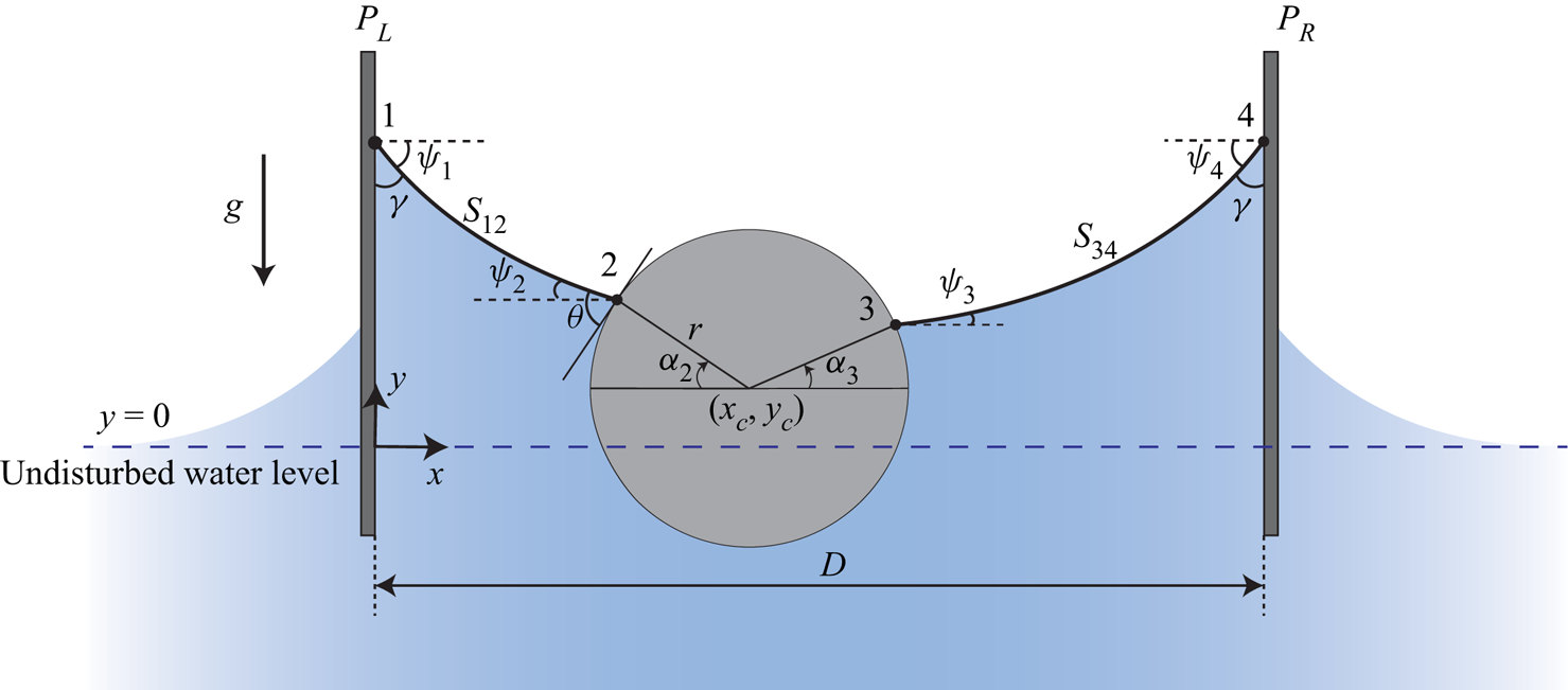
Figure 1. Schematic of the capillary system of a floating cylinder confined between two parallel vertical surface-piercing plates in a downward gravity field. The cylinder with a contact angle  $\theta $ is located at $({x_c}, {y_c})$. The contact angles of plate PL and plate PR are equal, denoted by $\gamma $. The distance between the two plates is denoted by D.
The inclination angles of the liquid surfaces at the four key contact points 1, 2, 3 and 4 are denoted by  ${\psi _i}$ (i = 1, 2, 3 and 4). At any point on a meniscus with the shape expressed as $y(x)$, the sign and magnitude of the inclination angle can be determined by ${\psi _i}= {\rm arctan}(\textrm{d}y/\textrm{d}\kern0.7pt x)$. For this situation as shown in this figure, ${\psi _1}$ and ${\psi _2}$ are negative while ${\psi _3}$ and ${\psi _4}$ are positive. Also, ${\alpha _2}$ and ${\alpha _3}$ denote the azimuthal angles of the contact points 2 and 3 on the cylinder, respectively; ${\alpha _2}({\alpha _3})$ is measured clockwise (counterclockwise) starting from the negative (positive) direction of the x axis, which are both positive for this figure; S 12 (S 34) is the meniscus at the left (right) side of the cylinder.
2.1. Young–Laplace equation in two dimensions
It is assumed that the menisci in the capillary system are in equilibrium. The height y(x) of the liquid surface is governed by the well-known Young–Laplace equation in two dimensions, which is given by
 \begin{equation}{\left( {\frac{{{y_x}}}{{\sqrt {1 + y_x^2} }}} \right)_x} = \kappa y.\end{equation}
In (2.1), the subscript x represents the derivative with respect to the coordinate x (i.e.  $(\cdot)_x \equiv {\rm d} (\cdot)/\textrm{d}\kern0.7pt x$), $\kappa$ is the capillary constant equal to ${\rho _l}g/\sigma $, where ${\rho _l}$ is the density difference between liquid and gas (while we neglect the density of gas in this paper), g is the gravitational acceleration and $\sigma $ is the surface tension coefficient. Bhatnagar & Finn (Reference Bhatnagar and Finn2016a) proposed a parametrization form of the Young–Laplace equation in two dimensions
 \begin{equation}\frac{{{\rm d}\kern0.06em x}}{{{\rm d}\psi }} = \frac{{\textrm{cos}\psi }}{{\kappa y}},\quad \frac{{{\rm d}y}}{{{\rm d}\psi }} = \frac{{\textrm{sin}\psi }}{{\kappa y}},\end{equation}
where the parameter  $\psi $ denotes the inclination angle of the interface $({\rm tan}\psi = \textrm{d}y/\textrm{d}\kern0.7pt x)$. A first integral of (2.2b) gives (Bhatnagar & Finn Reference Bhatnagar and Finn2016a; Zhou & Zhang Reference Zhou and Zhang2017)
 \begin{equation}\frac{\kappa }{2}{y^2}+ \textrm{cos}\psi = c \equiv \textrm{const}.\end{equation}
For a prescribed point  $({x^ \ast },{y^ \ast })$ at a meniscus, the integration constant c of the meniscus can be uniquely determined from (2.3) if the inclination angle ${\psi ^ \ast }$ of the meniscus at the prescribed point is also known. By explicitly integrating the terms of (2.2a,b), the solution curves of the Young–Laplace equation in two dimensions are given parametrically by
 \begin{gather}x - {x^ \ast }{\ =\ \pm }\frac{1}{{\sqrt {2\kappa } }}\int_{{\psi ^ \ast }}^\psi {\frac{{\textrm{cos}\tau \,\textrm{d}\tau }}{{\sqrt {c - \textrm{cos}\tau } }},} \quad \psi {\ \in }\left[ {{\psi^ \ast },\frac{{\rm \pi} }{2}} \right],\end{gather}
 \begin{gather}y ={\pm} \sqrt {\frac{{2(c - \textrm{cos}\psi )}}{\kappa }} .\end{gather}
From (2.4), it can be inferred that there are two corresponding solution curves for one integration constant c, as is shown in figure 12 in Appendix A. While the contact angle boundary conditions can be satisfied for only one of the two curves. After the integration constant c of a meniscus is obtained, the meniscus profile y(x) can be determined uniquely (see Appendix A).
The integration constants of the menisci S 12 and S 34 in figure 1 are denoted by  ${c_{12}}$ and ${c_{34}}$, respectively. From (2.3), ${c_{12}}({c_{34}})$ can be expressed in terms of the height and the inclination angle of the interface at contact point 2 (contact point 3). Also, we give ${c_{12}}({c_{34}})$ in terms of the height ${y_c}$ of the cylinder centre and the azimuthal angle ${\alpha _2}$ ( ${\alpha _3}$)
 \begin{align}{c_{12}} &= \frac{\kappa }{2}{({y_c} + r\sin {\alpha _2})^2} + \cos \left( { - {\alpha_2} - \theta + \frac{{\rm \pi} }{2}} \right),\end{align}
 \begin{align}{c_{34}} &= \frac{\kappa }{2}{({y_c} + r\sin {\alpha _3})^2} + \cos \left( {{\alpha_3} + \theta - \frac{{\rm \pi} }{2}} \right).\end{align}
 For two arbitrary points I and II on a meniscus, the horizontal distance  $d = |{x_{II}}-{x_I}|$ can be obtained from (2.4a). Zhou & Zhang (Reference Zhou and Zhang2017) proposed that the horizontal distance d can be expressed in a unified form with the elliptical integrals. Based on the inclination angles rather than the contact angles as used in Zhou & Zhang (Reference Zhou and Zhang2017), the horizontal distance d can be rewritten as a function about the integration constant c of the menisci from (2.4a)
 \begin{equation}d(c;{\psi _I},{\psi _{II}}) = \left|{\frac{1}{{\sqrt \kappa }}{\{ }a[E({\beta_{II}},k) - E({\beta_I},k)] - b[F({\beta_{II}},k) - F({\beta_I},k)]\} } \right|,\end{equation}
where  ${\psi _I}$ and ${\psi_{II}}$ denote the inclination angles of the meniscus at the two arbitrary points I and II, respectively, E and F are elliptical integrals of the first kind and the second kind, respectively, k represents the elliptical modules, ${\beta _I}$ and ${\beta _{II}}$ are the amplitudes for the two points I and II, respectively, and the parameters a, b, k, ${\beta _I}$ and ${\beta _{II}}$ are all given in table 1 in Appendix B.
2.2. Geometric constraints
For the contact points 1 and 4 on the plates, the inclination angles  ${\psi _1}$ and ${\psi _4}$ are related to the plates’ contact angle $\gamma $, while for the contact points 2 and 3 on the cylinder, the inclination angles ${\psi _i}$ (i = 2 and 3) are related to the cylinder's contact angle $\theta $ and the azimuthal angles ${\alpha _i}$ (i = 2 and 3). The four inclinations are expressed as
 \begin{gather}{\psi _1} = \gamma - \frac{{\rm \pi} }{2},\quad {\psi _4} ={-} \gamma + \frac{{\rm \pi} }{2},\end{gather}
 \begin{gather}{\psi _2} ={-} {\alpha _2} - \theta + \frac{{\rm \pi} }{2},\quad {\psi _3} = {\alpha _3} + \theta - \frac{{\rm \pi} }{2}.\end{gather}
In this work, we set  $- {\rm \pi}/2\le{\psi _i}{\ \le {\rm \pi}/}2$ (i = 1, 2, 3 and 4) and $- {\rm \pi}/2\le{\alpha _i}{\ \le {\rm \pi}/}2$ (i = 2 and 3).
With the cylinder located at  $({x_c},{y_c})$, the horizontal distance between the contact points 1 and 2 and the horizontal distance between the contact points 3 and 4 can both be expressed in terms of the function (2.6), which gives $d({c_{12}}; {\psi _1},{\psi _2})$ and $d({c_{34}}; {\psi _3},{\psi _4})$. Substituting (2.7a–d) into $d({c_{12}}; {\psi _1},{\psi _2})$ and $d({c_{34}}; {\psi _3},{\psi _4})$, the two horizontal distances satisfy the following relations:
 \begin{gather}d\left( {{c_{12}};\gamma - \frac{{\rm \pi} }{2}, - {\alpha_2} - \theta + \frac{{\rm \pi} }{2}} \right) = {x_c} - r\cos {\alpha _2},\end{gather}
 \begin{gather}d\left( {{c_{34}};{\alpha_3} + \theta - \frac{{\rm \pi} }{2}, - \gamma + \frac{{\rm \pi} }{2}} \right) = D - {x_c} - r\cos {\alpha _3},\end{gather}
where  ${c_{12}}({c_{34}})$ can be expressed in terms of ${y_c}$ and ${\alpha _2}({\alpha _3})$ from (2.5a,b). We set D > 2r and $r < {x_c} < D - r$ to ensure that the cylinder will not touch either plate.
2.3. Forces of the cylinder
For the floating cylinder with static menisci, the forces acting on it are the surface tension force  ${\boldsymbol{T}_2}$ at the contact point 2, the surface tension force ${\boldsymbol{T}_3}$ at the contact point 3, the pressure force P (due to hydrostatic pressure) and the weight force ${\boldsymbol{f}_g}$. The net force $\boldsymbol{f}$ exerted on the cylinder is given by
 \begin{equation}\boldsymbol{f} = {\boldsymbol{T}_2} + {\boldsymbol{T}_3} + \boldsymbol{P} + {\boldsymbol{f}_g}.\end{equation}
 The sum of the two horizontal components of the surface tension forces  ${\boldsymbol{T}_2}$ and ${\boldsymbol{T}_3}$ is given by
 \begin{equation}{T_{2h}} + {T_{3h}} = \sigma \cos \left( {{\alpha_3} + \theta - \frac{{\rm \pi} }{2}} \right) - \sigma \cos \left( { - {\alpha_2} - \theta + \frac{{\rm \pi} }{2}} \right).\end{equation}
The pressure force P can be calculated by integrating the hydrostatic pressure over the wetted cylinder surface (Keller Reference Keller1998). We have the horizontal component of P as
 \begin{equation}{P_h} = {\textstyle{1 \over 2}}{\rho _l}g{({y_c} + r\cos {\alpha _3})^2} - {\textstyle{1 \over 2}}{\rho _l}g{({y_c} + r\cos {\alpha _2})^2}.\end{equation}
The horizontal resultant force  ${f_h}$ is the sum of ${T_{2h}}$, ${T_{3h}}$ and ${P_h}$. From (2.5), ${f_h}$ can be expressed in terms of the integration constants ${c_{12}}$ and ${c_{34}}$
 \begin{equation}{f_h} = \sigma ({c_{34}} - {c_{12}}).\end{equation}
For an unconfined cylinder floating in an infinite bath (without plates), the horizontal balance is satisfied automatically for  ${c_{12}} = {c_{34}} = 1$ (Bhatnagar & Finn Reference Bhatnagar and Finn2016a; Zhang et al. Reference Zhang, Zhou and Zhu2018). Accordingly, the formula (2.12) of the horizontal resultant force can be generalized to the floating object of any shape whether it is confined or not.
Zhang et al. (Reference Zhang, Zhou and Zhu2018) proposed that the pressure force P can be decomposed into the buoyancy force and the compensating pressure force, which makes the calculation of the vertical resultant force  ${f_v}$ convenient. The formula of ${f_v}$ is given by (Zhang et al. Reference Zhang, Zhou and Zhu2018)
 \begin{equation}\begin{aligned} {f_v} & ={-} \dfrac{{{\rho _l}g}}{2}r(\cos {\alpha _2} + \cos {\alpha _3})(2{y_c} + r\sin {\alpha _2} + r\sin {\alpha _3})\\ & \quad - \sigma [\cos ({\alpha _2} + \theta ) + \cos ({\alpha _3} + \theta )] + {\rho _l}g\dfrac{{{\rm \pi} + {\alpha _2} + {\alpha _3} + \sin ({\alpha _2} + {\alpha _3})}}{2}{r^2} - {f_g}, \end{aligned}\end{equation}
where  ${f_g}$ denotes the norm of the weight force vector ${\boldsymbol{f}_g}$.
Provided that the liquid, the air and the cylinder (solid) are all homogeneous, the resultant moment exerted on the cylinder about its centre is always zero regardless of the position and shape of the contact line (Singh & Hesla Reference Singh and Hesla2004; Janssens et al. Reference Janssens, Chaurasia and Fried2017). Thus the rotational equilibrium of the cylinder is reached automatically. Equilibrium of the cylinder can be attained as long as both of the net force components  ${f_h}$ and ${f_v}$ vanish
 \begin{gather}\sigma ({c_{12}} - {c_{34}}) = 0,\end{gather}
 \begin{gather}\begin{array}{ccccc} & - \dfrac{{{\rho _l}g}}{2}r(\cos {\alpha _2} + \cos {\alpha _3})(2{y_c} + r\sin {\alpha _2} + r\sin {\alpha _3}) - \sigma [\cos ({\alpha _2} + \theta )\\ & \quad + \cos ({\alpha _3} + \theta )] + {\rho _l}g\dfrac{{{\rm \pi} + {\alpha _2} + {\alpha _3} + \sin ({\alpha _2} + {\alpha _3})}}{2}{r^2} - {f_g} = 0. \end{array}\end{gather}
2.4. Scaling
To facilitate the analysis below, a scaling is adopted in which lengths are measured relative to the capillary length  $\sqrt {1/\kappa }$, and forces are measured relative to ${\rm \pi} {r^2}{\rho _l}g$, i.e. the weight of the cylinder if its density equals ${\rho _l}$. The following dimensionless lengths and force components are used:
 \begin{gather}\{ \bar{x}, \bar{y}, \bar{r}, \bar{D}, {\bar{x}_c}, {\bar{y}_c}, \bar{d}(c; {\psi _I},{\psi _{II}})\} = \{ x, y, r, D, {x_c}, {y_c}, d(c; {\psi _I},{\psi _{II}})\} /\sqrt {1/\kappa } ,\end{gather}
 \begin{gather}\{ {\bar{f}_h},{\bar{f}_v},{\bar{f}_g}\} = \{ {f_h},{f_v},{f_g}\} /{\rm \pi} {r^2}{\rho _l}g.\end{gather}
In this scaling, the dimensionless weight  ${\bar{f}_g}$ is actually the ratio of the cylinder density ${\rho _s}$ to the liquid density ${\rho _l}$.
For the solution curves (2.4a,b) of the Young–Laplace equation in two dimensions, the dimensionless counterparts give
 \begin{gather}\bar{x} - {\bar{x}^ \ast } ={\pm} \frac{1}{{\sqrt 2 }}\int_{{\psi ^ \ast }}^\psi {\frac{{\cos \tau \,\textrm{d}\tau }}{{\sqrt {c - \cos \tau } }}} ,\quad \psi {\ \in }\left[ {{\psi^ \ast },\frac{{\rm \pi} }{2}} \right],\end{gather}
 \begin{gather}\bar{y} ={\pm} \sqrt {2(c - \cos \psi )} .\end{gather}
For (2.5a,b) determining the integration constants  ${c_{12}}$ and ${c_{34}}$, the dimensionless counterparts give
 \begin{align}{c_{12}} &= \frac{1}{2}{({\bar{y}_c} + \bar{r}\sin {\alpha _2})^2} + \cos \left( { - {\alpha_2} - \theta + \frac{{\rm \pi} }{2}} \right),\end{align}
 \begin{align}{c_{34}} &= \frac{1}{2}{({\bar{y}_c} + \bar{r}\sin {\alpha _3})^2} + \cos \left( {{\alpha_3} + \theta - \frac{{\rm \pi} }{2}} \right).\end{align}
For the distance function (2.6), we obtain the dimensionless form as
 \begin{equation}\bar{d}(c;{\psi _I},{\psi _{II}}) = |a[E({\beta _{II}},k) - E({\beta _I},k)] - b[F({\beta _{II}},k) - F({\beta _I},k)]|,\end{equation}
where the parameters a, b, k,  ${\beta _I}$ and ${\beta _{II}}$ (given in table 1 in Appendix B) are all dimensionless. For the geometric relationship (2.8a,b), we obtain
 \begin{gather}\bar{d}\left( {{c_{12}};\gamma - \frac{{\rm \pi} }{2}, - {\alpha_2} - \theta + \frac{{\rm \pi} }{2}} \right) = {\bar{x}_c} - \bar{r}\cos {\alpha _2},\end{gather}
 \begin{gather}\bar{d}\left( {{c_{34}};{\alpha_3} + \theta - \frac{{\rm \pi} }{2}, - \gamma + \frac{{\rm \pi} }{2}} \right) = \bar{D} - {\bar{x}_c} - \bar{r}\cos {\alpha _3}.\end{gather}
For the horizontal resultant force (2.12) and the vertical resultant force (2.13), we obtain
 \begin{gather}{\bar{f}_h} = {c_{34}} - {c_{12}},\end{gather}
 \begin{gather}\begin{aligned} {{\bar{f}}_v} & ={-} \dfrac{1}{{2{\rm \pi} \bar{r}}}(\cos {\alpha _2} + \cos {\alpha _3})(2{{\bar{y}}_c} + \bar{r}\sin {\alpha _2} + \bar{r}\sin {\alpha _3})\\ & \quad - \dfrac{{[\cos ({\alpha _2} + \theta ) + \cos ({\alpha _3} + \theta )]}}{{{\rm \pi} {{\bar{r}}^2}}} + \dfrac{{{\rm \pi} + {\alpha _2} + {\alpha _3} + \sin ({\alpha _2} + {\alpha _3})}}{{2{\rm \pi} }} - {{\bar{f}}_g}. \end{aligned}\end{gather}
For the equilibrium conditions (2.14a,b) of the cylinder, we obtain
 \begin{gather}{c_{12}} = {c_{34}},\end{gather}
 \begin{gather}\begin{aligned} & - \dfrac{1}{{2{\rm \pi} \bar{r}}}(\cos {\alpha _2} + \cos {\alpha _3})(2{{\bar{y}}_c} + \bar{r}\sin {\alpha _2} + \bar{r}\sin {\alpha _3}) - \dfrac{1}{{{\rm \pi} {{\bar{r}}^2}}}[\cos ({\alpha _2} + \theta ) + \cos ({\alpha _3} + \theta )]\\ & \quad + \dfrac{{{\rm \pi} + {\alpha _2} + {\alpha _3} + \sin ({\alpha _2} + {\alpha _3})}}{{2{\rm \pi} }} - {{\bar{f}}_g} = 0. \end{aligned}\end{gather}
3. Equilibrium analysis
For an unconfined cylinder horizontally floating in equilibrium in an infinite bath (without plates), the menisci at the two sides of the cylinder are symmetric about the vertical symmetry axis of the cross-section. The integration constants of the two menisci are both equal to 1 (Bhatnagar & Finn Reference Bhatnagar and Finn2006; Chen & Siegel Reference Chen and Siegel2018). However, this is not the case for the floating cylinder confined between the two plates. From the horizontal balance condition (2.22a), the integration constant  ${c_{12}}$ of the meniscus S 12 and the integration constant ${c_{34}}$ of the meniscus S 34 are equal but not necessarily equal to 1, which may lead to different equilibrium states.
All the equilibrium states including meniscus profiles can be obtained by solving (2.19) and (2.22) numerically (see Appendix C). According to the symmetry (or asymmetry) of the two menisci S 12 and S 34 at the two sides of the cylinder, the equilibrium solutions are classified into three types: the equilibrium solutions of fully symmetric menisci, the equilibrium solutions of partially symmetric menisci and the equilibrium solutions of asymmetric menisci. For the equilibrium of fully symmetric menisci, the two menisci S 12 and S 34 are fully symmetric about the vertical symmetry axis of the cross-section of the cylinder (see figure 2a,b). For the equilibrium of partially symmetric menisci, one meniscus is symmetric to part of another meniscus about the vertical symmetry axis of the cross-section of the cylinder (see figure 2c,d). For the equilibrium of asymmetric menisci, the two menisci S 12 and S 34 are asymmetric about the vertical symmetry axis of the cross-section of the cylinder (see figure 2e).

Figure 2. Different types of equilibrium states: (a,b) the equilibria of fully symmetric menisci, (c,d) the equilibria of partially symmetric menisci and (e) the equilibria of asymmetric menisci. Red solid curves represent parts of menisci symmetric to each other. Dashed curves demonstrate the equivalent equilibrium states. Physical parameters in (a-d) are the same, and are given by  $\bar{D} = 3$, $\bar{r} = 0.5$, $\gamma = {\rm \pi}/3$, $\theta = {\rm \pi}/2$ and ${\bar{f}_g} = 3.714$. There is no equilibrium of asymmetric menisci for the parameters given in (a–d). Physical parameters in (e) are the same as those in (a–d) except ${\bar{f}_g} = 0.595$.
3.1. Equilibria of fully symmetric menisci
Intuitively, there exists an equilibrium that the floating cylinder is located centrally between the two plates and the menisci at the two sides ( ${S_{12}}$ and ${S_{34}}$) are fully symmetric about the vertical symmetry axis of the cylinder's cross-section (see figure 2a,b). From the symmetry, it can be inferred that the azimuthal angles of the contact points 2 and 3 are equal. For the equilibria of fully symmetric menisci, we have ${\bar{x}_c}= \bar{D}/2$ and ${\alpha _2}= {\alpha _3}=\alpha $.
With fully symmetric menisci at the two sides, the resultant vertical force profiles of the unconfined cylinder floating in an infinite bath and the confined cylinder floating between two parallel vertical plates are shown in figure 3(a). We assume that all states in figure 3(a) are in equilibrium for there can exist an extra vertical body force (not the weight) to counteract the vertical unbalance with  ${\bar{f}_y}{\ \ne }0$. A good agreement of force profiles can be found between the unconfined case (in Zhang et al. Reference Zhang, Zhou and Zhu2018) and the confined case with $\bar{D}= 20\bar{r}$. Letting the vertical resultant force ${\bar{f}_y} = 0$ in figure 3(a), these equilibria can be reached spontaneously (without the extra body force), the menisci of which are depicted in figure 3(b). The weight ${\bar{f}_g} = 0.5$ of the cylinder is chosen in order that the weight force ${\boldsymbol{f}_g}$ balances the pressure force P alone at the equilibrium of the unconfined case. At this equilibrium state, the cylinder is half-immersed and the menisci at the two sides are flat, which can be expressed as $\bar{y}(\bar{x})= 0$ (see dashed line with red circles in figure 3b). For the confined cases, as the distance $\bar{D}$ between the two plates increases, the menisci in the vicinity of contact points on the cylinder get flat and the effect of plates on the cylinder diminishes gradually.

Figure 3. (a) Resultant vertical forces  ${\bar{f}_y}$ of confined and unconfined cases for different azimuthal angles ${\alpha _2} = {\alpha _3} = \alpha $, and (b) right menisci of confined and unconfined cases for ${\bar{f}_y} = 0$ in (a). The meniscus of the unconfined case (dashed line with red circles) is in a horizontal line across the centre of the cylinder. Each of the other menisci in (b) corresponds to the force profile in (a) with the same colour. The following parameters are given: $\bar{r} = 0.553$, ${\bar{f}_g} = 0.5$, $\theta = {\rm \pi}/2$ and $\theta = {\rm \pi}/4$.
There are at most two equilibria for an unconfined cylinder floating in an infinite bath (Chen & Siegel Reference Chen and Siegel2018). However, for a confined cylinder floating between two parallel vertical plates, there are possibly more than two equilibria. An example of three equilibria of fully symmetric menisci for a two-dimensional cylinder floating in a lateral finite container with a liquid volume constraint is shown by McCuan & Treinen (Reference Mccuan and Treinen2018). While, in this paper, there is no liquid volume constraint for the capillary system. The Young–Laplace equation of volume constraint is given by (Finn Reference Finn1986)
 \begin{equation}{\left( {\frac{{{Y_x}}}{{\sqrt {1 + Y_x^2} }}} \right)_x}= \kappa Y + \lambda ,\end{equation}
where Y denotes the meniscus height with volume constraint and  $\lambda$ is a constant related to the volume constraint. Comparing (2.1) and (3.1), we can obtain the relation that
 \begin{equation}Y(x) - y(x) = \lambda /\kappa .\end{equation}
For the capillary system with volume constraint,  $\lambda /\kappa$ denotes the height variation of the reference point where the hydrostatic pressure is zero. Apparently, the volume constraint may bring a vertical translation for the whole equilibrium configuration but it will not change the meniscus shape. After an equilibrium configuration without volume constraint (not necessarily with fully symmetric menisci) is determined, the equilibrium configuration with volume constraint can be obtained by finding the distance between the cylinder and the bottom of the container to satisfy the specific volume.
To validate our numerical method, the relation of the weight  ${\bar{f}_g}$ and the azimuthal angle $\alpha $ at the equilibria of fully symmetric menisci is depicted in figure 4(a). For ${\bar{f}_g} = 0.99$, the three equilibrium solutions about the azimuthal angle $\alpha $ (i.e. $\alpha = 0.013$, 0.215 and 0.613) are in a good agreement with those by McCuan & Treinen (Reference Mccuan and Treinen2018).

Figure 4. (a) Weight  ${\bar{f}_g}$ versus azimuthal angle $\alpha $ in the equilibria of fully symmetric menisci. The three blue circles correspond to the three equilibrium solutions for ${\bar{f}_g} = 0.99$ in McCuan & Treinen (Reference Mccuan and Treinen2018). It should be noted that the dimensionless weight ${\bar{f}_g}$ is equivalent to the density ratio in McCuan & Treinen (Reference Mccuan and Treinen2018). The red, orange, purple and green triangles represent four equilibrium states of ${\bar{f}_g} = 1.06$. Panel (b) shows the four equilibrium states of ${\bar{f}_g} = 1.06$. Each of the menisci (denoted by red, orange, purple or green curves, respectively) corresponds to the triangle with the same colour in (a). The following parameters are used: $\bar{D} = 8$, $\bar{r} = 3.996$, $\theta = {\rm \pi}/2$ and $\gamma = {\rm \pi}/2$.
Here and hereinafter, there can exist some equilibrium states of negative weight  ${\bar{f}_g}$ (see negative values of $\alpha $ in figure 4a), these are equivalent to cases in which there exists an extra upward body force on the cylinder, pulling the cylinder out of the bath (Benilov & Oron Reference Benilov and Oron2010). Further, we find that there can be at most four equilibrium solutions for ${\bar{f}_g} = 1.06$ in figure 4(a), the menisci of which are depicted in figure 4(b). Based on a comprehensive study, we find that three or four equilibria may occur only when the distance satisfies $2\bar{r} < \bar{D}\mathrm{\ \mathbin{\lower.3ex\hbox{$\buildrel< \over {\smash{\scriptstyle\sim}\vphantom{_x}}$}}\ }2.01\bar{r}$ and the radius satisfies $\bar{r}\mathrm{\ \mathbin{\lower.3ex\hbox{$\buildrel> \over {\smash{\scriptstyle\sim}\vphantom{_x}}$}}\ }3$. The floating cylinder can hardly move horizontally when $2\bar{r} < \bar{D}\mathrm{\ \mathbin{\lower.3ex\hbox{$\buildrel< \over {\smash{\scriptstyle\sim}\vphantom{_x}}$}}\ }2.01\bar{r}$, and the capillary effect is relatively weak with the radius much larger than the capillary length. As a result, the cases with more than two equilibrium solutions of fully symmetric menisci will not be focused on in the following sections. The cases of $\bar{D} = 1.1 \sim 3$ and $\bar{r} = 0.5$ with at most two equilibrium solutions of fully symmetric menisci will be mainly taken as examples to conduct further analysis.
The stability analysis is performed for the equilibrium points of  ${\bar{f}_g} = 0.99$ and 1.06 (denoted by circles and triangles, respectively, in figure 4a) in advance with the method in § 4. Under the effect of plates, the vertical stabilities of the equilibria of fully symmetric menisci are enhanced (see § 4.2), with the result that all points except the rightmost point of ${\bar{f}_g} = 1.06$ are vertically stable, while only the second equilibrium points (from left) of ${\bar{f}_g} = 0.99$ and ${\bar{f}_g} = 1.06$ are vertically stable and horizontally stable. Although the existence of a liquid volume constraint will not influence the equilibrium configuration, it can influence the stabilities of the equilibria, especially for the sensitive case $\bar{D}\mathrm{\ \approx }2\bar{r}$. The equilibrium point of ( $\alpha $, ${\bar{f}_g}$) = (0.215, 0.99) is vertically stable for the case without volume constraint in this paper, while this point is vertically unstable for the case with volume constraint as also shown in McCuan & Treinen (Reference Mccuan and Treinen2018).
3.2. Equilibria of partially symmetric menisci
For the equilibrium of partially symmetric menisci, the meniscus at one side is symmetric to part of the meniscus at the other side (see figure 2c,d). From symmetry, the azimuthal angles at the contact points 2 and 3 are also equal. Strictly speaking, the floating cylinder should not be located centrally between the two plates, otherwise this state belongs to the equilibria of fully symmetric menisci. For the equilibria of partially symmetric menisci, we have  ${\bar{x}_c}\mathrm{\ \ne }\bar{D}/2$ and ${\alpha _2} = {\alpha _3} = \alpha $.
At the equilibria of partially symmetric menisci, the horizontal position  ${\bar{x}_c}$ varies with the weight ${\bar{f}_g}$ of the cylinder. The solution curves of ${\bar{f}_g}$ versus ${\bar{x}_c}$ at these equilibria are shown in figure 5, supposing that the radius $\bar{r}$, the contact angle $\theta $ of the cylinder and the distance $\bar{D}$ between the two plates are all fixed. Several equilibrium points for ${\bar{x}_c} = \bar{D}/2$ on curves in figure 5 correspond to the equilibria of fully symmetric menisci rather than the equilibria of partially symmetric menisci, although we do not distinguish them particularly.

Figure 5. Solution curves of  ${\bar{f}_g}$ versus ${\bar{x}_c}$ at the equilibria of partially symmetric menisci: (a) discontinuous distribution mode ( $\gamma = 50^\circ $, 55°, 60° and 120°) and continuous distribution mode $(\gamma = 90^\circ )$, and (b) transition from the discontinuous distribution mode $(\gamma = 65^\circ )$ to the double-continuous mode ( $\gamma = 66^\circ $ and 67°) and the continuous distribution mode $(\gamma = 68^\circ )$. The following parameters are used: $\bar{D}= 3$, $\bar{r} = 0.5$ and $\theta = {\rm \pi}/2$.
From the solution curves for  ${\bar{f}_g}$ versus ${\bar{x}_c}$ in figure 5, it can be concluded that there exist four distribution modes: the continuous distribution mode, the double-continuous distribution mode, the discontinuous distribution mode and the no-distribution mode. For the continuous distribution mode (for example, $\gamma = 90^\circ $ in figure 5(a) and $\gamma = 68^\circ$ in figure 5(b)), there is only one solution curve which is continuous between $\bar{r}$ and $\bar{D} - \bar{r}$. For the double-continuous distribution mode (for example, $\gamma = 66^\circ$ and 67° in figure 5b), there is a lower, long solution curve and an upper, short solution curve. The longer solution curve is continuous between $\bar{r}$ and $\bar{D} - \bar{r}$. For the discontinuous distribution mode (for example, $\gamma = 50^\circ $, 55°, 60° and 120° in figure 5(a), and $\gamma = 65^\circ$ in figure 5(b)), there are two solution curves symmetric to each other about the line ${\bar{x}_c} = \bar{D}/2$. In this mode, the equilibria of partially symmetric menisci cannot appear for a medium value of ${\bar{x}_c}$ between $\bar{r}$ and $\bar{D} - \bar{r}$. While for the no-distribution mode, the equilibria of partially symmetric menisci can never be reached and there is no such solution curve for ${\bar{f}_g}$ versus ${\bar{x}_c}$, which occurs when $\gamma < 40^\circ$ with other parameters being the same as in figure 5(a).
On the solution curve of the double-continuous distribution mode or the discontinuous distribution mode, there can be two equilibrium points for one horizontal position  ${\bar{x}_c}$, such as points A and B in figure 5(a). Interestingly, parts of the meniscus profile of the equilibrium point A are the same as those of the equilibrium point B, which is illustrated in the corresponding inset. The solution curve for $\gamma = 90^\circ $ is the line ${\bar{f}_g} = 0.5$. At the equilibrium points on the line ${\bar{f}_g} = 0.5$, the menisci are flat and the horizontal displacement will not change the equilibrium, which is shown in the corresponding inset of $\gamma = 90^\circ $. For two supplementary contact angles, such as $\gamma = 60^\circ $ and 120° in figure 5(a), the two corresponding solution curves are symmetric about the line ${\bar{f}_g} = 0.5$. Two equilibrium points symmetric about the line ${\bar{f}_g} = 0.5$ correspond to two equilibrium configurations that are symmetric about the undisturbed liquid surface $\bar{y}=0$ (see the points C and C’, and the corresponding inset in figure 5a). In fact, for any equilibrium configuration with a given plates’ contact angle $\gamma = {\gamma ^ \ast }$, no matter what type this equilibrium is (i.e. not limited to the equilibrium of partially symmetric menisci), there must be another equilibrium configuration with plates’ contact angle $\gamma {\ =\ {\rm \pi}-\ }{\gamma ^ \ast }$ symmetric to this configuration about the line $\bar{y} = 0$, only if $\theta = {\rm \pi}/2$. The reason is because the two symmetric configurations can both satisfy the geometry relation (2.19).
For the equilibria of partially symmetric menisci, the distribution mode depends on not only the plates’ contact angle  $\gamma $ but also the distances $\bar{D}$ between the plates. The phase diagram of the four distribution modes in the parameter space $(\gamma , \bar{D})$ is shown in figure 6, assuming that the radius $\bar{r}$ and the contact angle $\theta $ of the cylinder are both fixed. The whole phase diagram is symmetric with respect to the line $\gamma {\ =\ {\rm \pi}/2}$ in figure 6. This is attributed to the symmetry of the two equilibrium solution curves for $\gamma ={\gamma ^ \ast }$ and $\gamma {\ =\ {\rm \pi}-\ }{\gamma ^ \ast }$(for example, $\gamma = 60^\circ $ and 120° in figure 5a). As the plates’ contact angle $\gamma $ increases (or decreases) from $\gamma = {\rm \pi}/2$, the continuous distribution mode (black point) turns into the double-continuous distribution mode (grey point), the discontinuous distribution mode (circle) and then, finally, the no-distribution mode (triangle). The continuous distribution mode (black point) is more likely to occur when the distance $\bar{D}$ between the two plates is small. The double-continuous distribution mode (grey point) is a transition of the continuous distribution mode (black point) and the discontinuous mode (circle), which occurs in a very small range of $\gamma $ values.

Figure 6. Phase diagram of distribution modes for the equilibria of partially symmetric menisci in a parameter space  $(\gamma, \bar{D})$. The continuous distribution mode, the double-continuous distribution mode, the discontinuous distribution mode and the no-distribution mode are denoted by black points, grey points, circles and triangles, respectively. The double-continuous distribution mode lies near the grey dashed curves. The following physical parameters of the cylinder are used: $\bar{r} = 0.5$ and $\theta = {\rm \pi}/2$. The distribution modes in figure 5(a,b) can be checked by letting $\bar{D}=3$ in this figure.
3.3. Equilibria of asymmetric menisci
The above two types of equilibrium states are both based on the precondition that the menisci at the two side of the cylinder are (partially) symmetric to each other. However, there can be equilibrium states with asymmetric menisci at the two sides of the cylinder (see figure 2e). For the equilibria of asymmetric menisci, we have  ${\alpha _2}\mathrm{\ \ne }{\alpha _3}$.
For the equilibria of asymmetric menisci, the horizontal position  ${\bar{x}_c}$ also varies with the weight ${\bar{f}_g}$ of the cylinder. The solution curves of ${\bar{f}_g}$ versus ${\bar{x}_c}$ at the equilibria of asymmetric menisci are shown in figure 7. Also, the equilibrium points for ${\bar{x}_c}=\bar{D}/2$ on curves in figure 7 correspond to the equilibria of fully symmetric menisci rather than the equilibria of asymmetric menisci, while there is no need to distinguish these points particularly. The points on the solution curve for $\gamma = {\rm \pi}/2$ (i.e. ${\bar{f}_g} = 0.5$, blue dashed line) actually correspond to the equilibria of partially symmetric menisci (see also $\gamma = {\rm \pi}/2$ in figure 5a). Strictly speaking, there are no equilibria of asymmetric menisci for $\gamma = {\rm \pi}/2$.

Figure 7. Solution curves of  ${\bar{f}_g}$ versus ${\bar{x}_c}$ at the equilibria of asymmetric menisci. The plates’ contact angle $\gamma $ gets larger from 0 to ${\rm \pi} $ with an increment of ${\rm \pi}/18$. The curve ${\bar{f}_g} = 0.5$ (dashed blue line) is exactly the curve for $\gamma = {\rm \pi}/2$ in figure 5(a). The points on ${\bar{f}_g} = 0.5$ correspond to the equilibria of partially symmetric menisci. Symmetric about ${\bar{f}_g} = 0.5$, the equilibrium points A and A’ are on the two curves for $\gamma = 5{\rm \pi}/18$ and $\gamma = 13{\rm \pi}/18$, respectively. The following parameters are used: $\bar{D} = 3$, $\bar{r} = 0.5$ and $\theta = {{\rm \pi} /2}$.
Two solution curves with plates’ contact angles supplementary to each other (such as the curves for  $\gamma =0$ and $\gamma {\ =\ {\rm \pi}}$ in figure 7) are symmetric about the line ${\bar{f}_g} = 0.5$. The two equilibrium points symmetric about the line ${\bar{f}_g} = 0.5$ correspond to the two equilibrium states that are symmetric about the undisturbed liquid surface $\bar{y} = 0$ (see the points A and A’, and the corresponding inset). On a solution curve with a prescribed $\gamma $, there can be only one equilibrium point for an arbitrary horizontal position ${\bar{x}_c}$ between $\bar{r}$ and $\bar{D} - \bar{r}$, which is similar to the continuous distribution mode of the equilibria of partially symmetric menisci.
4. Stability
Based on the equilibrium states of the confined floating cylinder, the stabilities are discussed. In § 4.1, the two-dimensional stability conditions of the capillary system are presented, and the relation between the two-dimensional stability conditions and the one-dimensional (horizontal or vertical) stability condition is discussed. In § 4.2, comparing with the vertical stabilities in the unconfined cases (without plates), a new vertical stability mechanism of the equilibria of fully symmetric menisci in the confined cases is found. In § 4.3, the two-dimensional stabilities of the confined floating cylinder are studied, including the effect of the new mechanism (discussed in § 4.2) on the two-dimensional stabilities.
4.1. Stability conditions
A stable cylinder floating between two parallel vertical stationary plates means that the cylinder can resist infinitesimal disturbance of any direction (not limited to the horizontal direction and the vertical direction) in the two-dimensional plane. From the principle of virtual work, neglecting dissipation, the energy functional E of the whole capillary system in equilibrium satisfies  $\delta E = 0$. The floating cylinder in equilibrium is stable if the second variation of the energy functional E is positive, i.e. the energy functional reaches a local minimum as (Erdös et al. Reference Erdös, Schibler and Herndon1992a)
 \begin{equation}{\delta ^2}E = \sum\limits_{i = 1}^n {\sum\limits_{j = 1}^n {\left( {\frac{{{\partial^2}E}}{{\partial {q_i}{q_j}}}} \right)\delta {q_i}\delta {q_j}} } > 0,\end{equation}
where  ${q_i}({q_j})$ denotes the degree of freedom in the system and n denotes the number of degrees of freedom. Degrees of freedom of the capillary system in this paper are the cylinder's horizontal position ${\bar{x}_c}$, and vertical position ${\bar{y}_c}$. The inequality (4.1) is equivalent to the condition that the Hessian matrix $[{\partial ^2}E/\partial {q_i}\partial {q_j}]$ is positive–definite. The leading principal minors of the positive–definite matrix are positive, which gives the stability conditions as
 \begin{gather}\frac{{{\partial ^2}\bar{E}}}{{\partial \bar{x}_c^2}} > 0,\end{gather}
 \begin{gather}\frac{{{\partial ^2}\bar{E}}}{{\partial {{\bar{x}}_c}^2}}\frac{{{\partial ^2}\bar{E}}}{{\partial {{\bar{y}}_c}^2}} - {\left( {\frac{{{\partial^2}\bar{E}}}{{\partial {{\bar{x}}_c}\partial {{\bar{y}}_c}}}} \right)^2} > 0,\end{gather}
where  $\bar{E}=E/({\rm \pi} {r^2}{\rho _l}g\sqrt {1/\kappa } )$, denoting the dimensionless energy of the capillary system.
To obtain the energy  $\bar{E}$ directly in (4.2a,b) is feasible but laborious, and it can be circumvented by the relation of energy and force. The relation between surface energy and surface forces can be seen in Finn (Reference Finn2006). The first variations of $\bar{E}$ with respect to the horizontal position ${\bar{x}_c}$ and the vertical position ${\bar{y}_c}$ of the cylinder are related to the net forces ${\bar{f}_h}$ and ${\bar{f}_v}$ on the cylinder (Kralchevsky et al. Reference Kralchevsky, Paunov, Denkov, Ivanov and Nagayama1993; Zhou & Zhang Reference Zhou and Zhang2017; Chen & Siegel Reference Chen and Siegel2018), respectively,
 \begin{equation}\frac{{\partial \bar{E}}}{{\partial {{\bar{x}}_c}}} ={-} {\bar{f}_h},\quad \frac{{\partial \bar{E}}}{{\partial {{\bar{y}}_c}}} ={-} {\bar{f}_v}.\end{equation}
The validity of (4.3a) and (4.3b) has been shown for the one-dimensional capillary system in Kralchevsky et al. (Reference Kralchevsky, Paunov, Denkov, Ivanov and Nagayama1993) and in Chen & Siegel (Reference Chen and Siegel2018), respectively. This implies that, from the aspect of statics, the capillary system is conservative when the viscous dissipation and the contact angle hysteresis are neglected. The total energy  $\bar{E}$ is the sum of all the potential energies (free surface energy, wetting energy and gravitational potential energy), and only related to the position of the cylinder. Regarding the net forces ${\bar{f}_h}$ and ${\bar{f}_v}$ as the potential forces, (4.3a,b) can also be derived for the two-dimensional conservative system (Hand & Finch Reference Hand and Finch1998). Thereby, the Hessian matrix to predict two-dimensional stability of the floating cylinder can be expressed as
 \begin{equation}\boldsymbol{\mathsf{H}}= \left( {\begin{array}{*{20}{c}} { - \dfrac{{\partial {{\bar{f}}_h}}}{{\partial {{\bar{x}}_c}}}}&{ - \dfrac{{\partial {{\bar{f}}_h}}}{{\partial {{\bar{y}}_c}}}}\\ { - \dfrac{{\partial {{\bar{f}}_v}}}{{\partial {{\bar{x}}_c}}}}&{ - \dfrac{{\partial {{\bar{f}}_v}}}{{\partial {{\bar{y}}_c}}}} \end{array}} \right).\end{equation}
For the symmetry of the Hessian matrix, we have  $\partial {\bar{f}_h}/\partial {\bar{y}_c} = \partial {\bar{f}_v}/\partial {\bar{x}_c} = {\partial ^2}\bar{E}/\partial {\bar{x}_c}\partial {\bar{y}_c}$. The relation of $\partial {\bar{f}_h}/\partial {\bar{y}_c} = \partial {\bar{f}_v}/\partial {\bar{x}_c}$ has been verified numerically. The stability conditions (4.2a,b) can be expressed as
 \begin{gather}\frac{{\partial {{\bar{f}}_h}}}{{\partial {{\bar{x}}_c}}} < 0,\end{gather}
 \begin{gather}\frac{{\partial {{\bar{f}}_h}}}{{\partial {{\bar{x}}_c}}}\frac{{\partial {{\bar{f}}_v}}}{{\partial {{\bar{y}}_c}}} - {\left( {\frac{{\partial {{\bar{f}}_h}}}{{\partial {{\bar{y}}_c}}}} \right)^2} > 0.\end{gather}
 If the cylinder is at an equilibrium of fully symmetric menisci with  ${\bar{f}_h} = 0$ and ${\bar{f}_v} = 0$, it is clear that a vertical displacement disturbance $\delta {\bar{y}_c}$ will bring a vertical force variation $\delta {\bar{f}_v}$ but the horizontal resultant force ${\bar{f}_h}$ stays zero, i.e. $\partial {\bar{f}_h}/\partial {\bar{y}_c} = 0$. Substituting $\partial {\bar{f}_h}/\partial {\bar{y}_c} = 0$ into (4.5a,b), the stability conditions for the equilibria of fully symmetric menisci can be simplified into
 \begin{gather}\frac{{\partial {{\bar{f}}_h}}}{{\partial {{\bar{x}}_c}}} < 0,\end{gather}
 \begin{gather}\frac{{\partial {{\bar{f}}_v}}}{{\partial {{\bar{y}}_c}}} < 0.\end{gather}
 For the capillary system with only the degree of freedom in the horizontal position  ${\bar{x}_c}$ (Zhou & Zhang Reference Zhou and Zhang2017), the stability condition is reduced to the horizontal stability condition (4.6a). For the capillary system with only the degree of freedom in the vertical position ${\bar{y}_c}$ (Chen & Siegel Reference Chen and Siegel2018; Zhang et al. Reference Zhang, Zhou and Zhu2018), the stability condition is reduced to the horizontal stability condition (4.6b). In particular, the equilibria of fully symmetric menisci, if the cylinder is both horizontally stable and vertically stable, are stable in two dimensions, while for the equilibria of partially symmetric menisci or asymmetric menisci, a horizontally stable and vertically stable cylinder can still be unstable in two dimensions when the energy of the whole system reaches a saddle point rather than a minimum point (Seydel Reference Seydel2009).
For an arbitrary equilibrium state with  ${\bar{f}_h} = 0$ and ${\bar{f}_v} = 0$ in the confined case, it is feasible to calculate the Hessian matrix in (4.4) numerically. With a small horizontal displacement disturbance $\delta {\bar{x}_c}$ or a small vertical displacement disturbance $\delta {\bar{y}_c}$, the corresponding force variations $\delta {\bar{f}_h}$ and $\delta {\bar{f}_v}$ can be calculated from (2.20) and (2.21), respectively. Therefore, the elements in the Hessian matrix (4.4) can all be obtained. With the Hessian matrix known, stability of this equilibrium can be predicted by (4.5a,b). The bifurcation theory (Seydel Reference Seydel2009) is applied to predict the stabilities of equilibria in this paper, and with the bifurcation theory, there is no need to calculate the Hessian matrix for every equilibrium point.
4.2. New mechanism of vertical stability
For the equilibrium of fully symmetric menisci, its vertical stability is decoupled from its horizontal stability because a vertical displacement will not break the horizontal force balance. Before studying the two-dimensional stabilities of all three types of equilibria, the vertical stabilities of the equilibria of fully symmetric menisci are discussed in this section. Comparing with the vertical stabilities in the unconfined case (without plates), a new vertical stability mechanism is found (figure 8). This mechanism has an important effect on the two-dimensional stabilities of equilibria in the confined case, which we will discuss in the next section.

Figure 8. (a) Relation of  ${\bar{f}_g}$ and ${\bar{y}_c}$ at the equilibria of fully symmetric menisci. The black curves and the blue curves denote vertically stable equilibria, while the red curves denote vertically unstable equilibria. The point A denotes the state of $\alpha = {\ -\ {\rm \pi}/}2$, the point B denotes the state of $\alpha = {\rm \pi}/2$ and the point O denotes the states of the half-immersed cylinder with flat menisci. The two solution curves with plates’ contact angles supplementary to each other (such as $\gamma {\ =\ {\rm \pi}/}18$ and $\gamma {\ =\ 17{\rm \pi} /}18$) are symmetric about the point O where $({\bar{x}_c},{\bar{y}_c},{\bar{f}_g}) = (\bar{D}/2,0,0.5)$. The following parameters are used: $\bar{D} = 2$, $\bar{r} = 0.5$ and $\theta = {{\rm \pi} /2}$. (b) Phase diagram of the equilibrium solutions of fully symmetric menisci with the first and the second vertical stability regions (denoted by pentagrams) and with only the first vertical stability region (denoted by squares), in a parameter space $(\gamma ,\bar{D})$ for $\bar{r} = 0.5$ and $\theta = {{\rm \pi} /2}$. The occurrence of the second stability region for different $\gamma $ in (a) can be checked by letting $\bar{D} = 2$ in (b).
For a cylinder at the equilibrium of fully symmetric menisci, the cylinder is vertically stable if it can resist an infinitesimal vertical force disturbance  $\delta {\bar{f}_v}$ (i.e. $\delta {\bar{f}_v}/\delta {\bar{y}_c} < 0$). We regard the vertical force disturbance $\delta {\bar{f}_v}$ as the weight disturbance $\delta {\bar{f}_g}$. Therefore, the relation of the weight ${\bar{f}_g}$ and the vertical height ${\bar{y}_c}$ at equilibria can also be used to predict the vertical stability. For the equilibria of fully symmetric menisci, the vertical stability condition (4.6b) is equivalent to ${\rm d}{\bar{f}_g}/{\rm d}{\bar{y}_c} < 0$, where ${\bar{f}_g}$ is the equilibrium weight of the cylinder at the vertical position ${\bar{y}_c}$.
The relation of  ${\bar{f}_g}$ and ${\bar{y}_c}$ at the equilibria of fully symmetric menisci is depicted in figure 8(a). On every curve for ${\bar{f}_g}$ versus ${\bar{y}_c}$, an equilibrium point is stable if ${\rm d}{\bar{f}_g}/{\rm d}{\bar{y}_c} < 0$. For plates’ contact angle $\gamma = {\rm \pi}/2$, only the region with a medium value of ${\bar{y}_c}$ (black curve) is vertically stable. For plates’ contact angle $\gamma = {{\rm \pi} /18}$ or $17{\rm \pi}/18$, there exists a second vertical stability region (blue curve) satisfying ${\rm d}{\bar{f}_g}/{\rm d}{\bar{y}_c} < 0$. In the confined cases, there can be at most two vertical stability regions for the equilibrium solutions of fully symmetric menisci, which is due to the capillary effect of the plates, while in the unconfined cases, there can be only one vertical stability region (see the thick curve in figure 8).
For an unconfined cylinder floating in an infinite bath, it was proven by Chen & Siegel (Reference Chen and Siegel2018) that the azimuthal angle  $\alpha $ of contacts points on the cylinder monotonically decreases as the height of the cylinder ${\bar{y}_c}$ increases. As a result, the condition for vertical stability ${\rm d}{\bar{f}_g}\textrm{/d}\alpha > 0$ is equivalent to ${\rm d}{\bar{f}_g}/{\rm d}{\bar{y}_c} < 0$ in the unconfined case. However, the condition ${\rm d}{\bar{f}_g}/{\rm d}\alpha > 0$ may not work for a confined floating cylinder (at the equilibria of fully symmetric menisci). For curves in figure 8(a), the azimuthal angle $\alpha $ keeps increasing from the right endpoints (corresponding to $\alpha = {\ -\ {\rm \pi}/}2$, see the inset of point A) to the left endpoints (corresponding to $\alpha = {\rm \pi}/2$, see the inset of point B). From (2.21), the equilibrium state of $\alpha = {\rm \pi}/2$ or $\alpha = {\ -\ {\rm \pi}/}2$ corresponds to a constant value of ${\bar{f}_g}$ no matter what value the contact angle $\gamma $ is. Obviously, $\alpha $ is still monotonically decreasing for ${\bar{y}_c}$ in the cases with only one vertical stability region. However, in the cases with two vertical stability regions, $\alpha $ is not monotonically decreasing for ${\bar{y}_c}$ and there can be two azimuthal angles $\alpha $ corresponding to one ${\bar{y}_c}$ (see the inset of points C and D).
From the point of view of bifurcation theory, we can also deem figure 8(a) as the bifurcation diagram of (2.22b) which can be used to predict the stabilities. Slightly different from much of the literature (Seydel Reference Seydel2009; Karasslanli Reference Karasslanli2012), the bifurcation parameter  ${\bar{f}_g}$ here is set on the longitudinal axis. The relation of ${\bar{f}_g}$ versus ${\bar{y}_c}$ depicted in figure 8(a) can be expressed as an implicit function ${\bar{f}_g}({\bar{y}_c})$. There is in general a change of stability at the bifurcation where the solution number of the equation ${\bar{f}_g}({\bar{y}_c})= \textrm{const}.$ changes (Seydel Reference Seydel2009). At the point with a maximum or minimum value of ${\bar{f}_g}$, the stability changes with the solution number changing from 0 to 2. At the intersection of the unstable region (red curve) and the second stable region (blue curve), the stability changes but the solution number remains 2. The reason lies in the singularity at the intersection point. At the intersection point $(\bar{y}_c^\ast ,\bar{f}_g^\ast )$, we have $\textrm{d}{\bar{f}_g}/\textrm{d}{\bar{y}_c}{|_{(\bar{y}_c^\ast ,\bar{f}_g^\ast )}}=\infty$. From implicit function theorem (Seydel Reference Seydel2009), the implicit function ${\bar{f}_g}({\bar{y}_c})$ can be extended until a singular point. Therefore, the singular point $(\bar{y}_c^\ast ,\bar{f}_g^\ast )$ splits the whole solution curve into two branches, whose bifurcation behaviours are independent of each other.
Supposing that the radius  $\bar{r}$ and the contact angle $\theta $ of the cylinder are both fixed, for the equilibrium solutions of fully symmetric menisci, the occurrence of the second vertical stability region for $({\bar{y}_c},{\bar{f}_g})$ depends on the plates’ contact angle $\gamma $ and the distance $\bar{D}$ between the two plates. The phase diagram of two vertical stability regions (denoted by pentagrams) and only one vertical stability region (denoted by squares) in a parameter space $(\gamma ,\bar{D})$ is shown in figure 8(b). The second vertical stability region (blue curves in figure 8a) is more likely to occur when the contact angle $\gamma $ is far from ${\rm \pi}/2$ or the distance $\bar{D}$ is small. We find that the distance $\bar{D}$ is more vital for the occurrence of the second vertical stability region. At a small enough $\bar{D}$ ( $\bar{D} < 1.56$ in figure 8b), the second vertical stability region occurs for an arbitrary $\gamma $. While at a large enough $\bar{D}$ ( $\bar{D} > 2.51$ in figure 8b), the second vertical stability region will never occur.
4.3. Two-dimensional stability
In practice, the floating cylinder in the confined case is stable only if it can resist infinitesimal disturbance of any direction (not limited to the horizontal direction and vertical direction) in two dimensions. For the three types of equilibria, their two-dimensional stabilities are predicted by the bifurcation theory in this section. Supposing that the plate's contact angle  $\gamma $, the cylinder's contact angle $\theta $, the distance $\bar{D}$ between the two plates and the radius $\bar{r}$ of the cylinder are all fixed, the weight ${\bar{f}_g}$ of the cylinder is selected as the bifurcation parameter. From § 3, it is clear that ${\bar{f}_g}$ can influence not only the vertical balance but also the horizontal balance, which makes ${\bar{f}_g}$ a proper bifurcation parameter in the two-dimensional system. As ${\bar{f}_g}$ varies, the equilibrium position $({\bar{x}_c},{\bar{y}_c})$ of the cylinder can be determined by solving (2.19) and (2.22). The bifurcation diagrams of $({\bar{x}_c},{\bar{y}_c})$ versus ${\bar{f}_g}$ for different values of $\bar{D}$ and $\gamma $ are illustrated in figure 9.

Figure 9. Bifurcation diagrams for  $({\bar{x}_c},{\bar{y}_c})$ versus ${\bar{f}_g}$: (a–e) with only one two-dimensional stability region, and (f) with two two-dimensional stability regions. The main bifurcation behaviour in (f) is the same as in (a). The other four diagrams with two stable regions whose main bifurcation behaviour is the same as in (b–e) are not given here. Solid (dashed) curves denote that the cylinder at equilibrium is stable (unstable) in two dimensions. Black, red and green curves represent the equilibrium solutions of fully symmetric menisci, partially symmetric menisci and asymmetry menisci, respectively. The two plates’ spacing is given by: (a–e) $\bar{D} = 3$, and (f) $\bar{D} = 2$. The plates’ contact angle is given by: (a) $\gamma = 2{\rm \pi}/9$, (b) $\gamma = {\rm \pi}/3$, (c) $\gamma = {11{\rm \pi} /30}$, (d) $\gamma = {4{\rm \pi} /}9$, (e) $\gamma = {\rm \pi}/2$ and (f) $\gamma = {\rm \pi}/6$. The other parameters used in (a–f) are: $\bar{r} = 0.5$ and $\theta = {{\rm \pi} /2}$.
Every panel in figure 9 is formed by the three types of equilibrium solutions, i.e. the equilibrium solutions of fully symmetric menisci (black curves), the equilibrium solutions of partially symmetric menisci (red curves) and the equilibrium solutions of asymmetric menisci (green curves). The bifurcation points (the extreme points or intersection points) split the solution curves in a bifurcation diagram into different branches, where the stabilities of all the points on a branch are the same (Seydel Reference Seydel2009; Zhou & Zhang Reference Zhou and Zhang2017).
Solid curves and dashed curves in figure 9 denote two-dimensional stable equilibria and two-dimensional unstable equilibria, respectively. The bifurcation behaviour in the diagrams is similar to the subcritical pitchfork bifurcation for one-dimensional stability problems (Seydel Reference Seydel2009), where only the trivial solutions can be stable. Here, the trivial solutions are the equilibrium solutions of fully symmetric menisci with  ${\bar{x}_c} = \bar{D}/2$ (black curve). In the three types of equilibrium solutions, only the equilibrium solutions of fully symmetric menisci could be stable in two dimensions.
The equilibrium solutions of asymmetric menisci (green curves) and the equilibrium solutions of partially symmetric menisci (red curves) influence the bifurcation points in a bifurcation diagram. For the curve of the equilibrium solutions of asymmetric menisci, there is always a bifurcation point (green point) at the intersection with the curve of equilibrium solutions of fully symmetric menisci. However, for the curve of the equilibrium solutions of partially symmetric solutions, the corresponding bifurcation point depends on the distribution mode. Judging from the relation of  ${\bar{x}_c}$ and ${\bar{f}_g}$ (see the examples in figure 6), the equilibrium solutions in figure 9(a–d) correspond to the no-distribution mode, the discontinuous distribution mode, the double-continuous distribution mode and the continuous mode, respectively. Also, the equilibrium solutions in figure 9(e,f) correspond to the continuous distribution mode and the no-distribution mode, respectively.
Five representative types of bifurcation diagrams with only one stable region are shown in figure 9(a–e). For a small value of  $\gamma $ (in figure 9a), the equilibrium solutions of partially symmetric menisci correspond to the no-distribution mode. The corresponding bifurcation point (black point) is the maximum point of ${f_g}$ on the curve of the equilibrium solutions of fully symmetric menisci. As $\gamma $ gets larger, the discontinuous distribution mode, the double-continuous distribution mode and the continuous distribution mode appear in figure 9(b–d), respectively. The corresponding bifurcation point changes from the maximum point of ${f_g}$ (black point) to the intersection point (red point). The shorter solution curve of the double-continuous distribution mode (shorter red curve in figure 9c) has no effect on the bifurcation behaviour. For $\gamma = {\rm \pi}/2$ (in figure 9e), strictly speaking, there are no equilibrium solutions of asymmetric menisci, and the equilibrium solutions of partially symmetric menisci correspond to the line ${\bar{f}_g} = 0.5$ (see also $\gamma = {\rm \pi}/2$ in figures 5a and 7). Visually, the green curve overlaps with the red curve in figure 9(e), meaning that there is no stable region remaining between the green curve and the red curve. As for $\gamma > {\rm \pi}/2$, there is no new type of bifurcation diagram beyond the five distinct types as shown in figure 9(a–e).
Looking back to figure 8(b), for  $\bar{D} = 3$ (in figure 9a–e), there is always only one vertical stability region on the equilibrium solutions of fully symmetric menisci. However, for $\bar{D} = 2$ and $\gamma = {\rm \pi}/6$ (in figure 9f), there are two vertical stability regions. The equilibrium solution curves of fully symmetric menisci for $({\bar{y}_c},{\bar{f}_g})$ in figure 9(a,f) are plotted in figure 10. If an equilibrium point is stable in two dimensions (on solid curves in figure 9 or 10), it must be vertically stable (i.e. satisfying ${\rm d}{\bar{f}_g}/{\rm d}{\bar{y}_c} < 0$, see also figure 8a). It is evident that the two-dimensional stability region is part of the vertical stability region of the equilibrium solutions of fully symmetric menisci, because the vertical stability is the precondition of the two-dimensional stability.

Figure 10. Equilibrium solution curves of fully symmetric menisci for  $({\bar{y}_c},{\bar{f}_g})$: (a) a side view of figure 9(a), and (b) a side view of figure 9(f). Solid (dashed) curves denote that the cylinder is stable (unstable) in two dimensions. The coloured points are exactly the points with the same colour in figures 9(a) and 9(f).
Similar to figure 9(a), the equilibrium solutions of partially symmetric menisci in figure 9(f) also correspond to the no-distribution mode. The main bifurcation behaviour in figure 9(f) is the same as in figure 9(a), except that the second vertical stability region (shorter solid black curve in figure 9f or 10b) is also stable in two dimensions. With further calculation of other parameters, we find that the second vertical stability region of the equilibrium solutions of fully symmetric menisci is always stable in two dimensions, while the main bifurcation behaviour will not get beyond the five types in figure 9(a–e). A significant conclusion is drawn that the second vertical stability region is also the second two-dimensional stability region.
From the bifurcation diagrams in figure 9, only the cylinder located centrally between the plates (at the equilibria of fully symmetric menisci) could be stable in two dimensions and its weight  ${\bar{f}_g}$ determines whether it is stable or not. The two-dimensional stability range of ${\bar{f}_g}$ with different plates’ contact angles $\gamma $ is shown in figure 11. This range of ${\bar{f}_g}$ is symmetric about the point $(\gamma ,{\bar{f}_g}) = ({\rm \pi} /2,0.5)$, resulting from the symmetry of two equilibrium solutions with $\gamma ={\gamma ^ \ast }$ and $\gamma {\ =\ {\rm \pi}-\ }{\gamma ^ \ast }$ (see example for $\gamma = 60^\circ $ and 120° in figure 5).

Figure 11. Stable range of  ${\bar{f}_g}$ at the equilibria of fully symmetric menisci: (a) the case with one two-dimensional stability region for $\bar{D} = 3$, and (b) the case with two two-dimensional stability regions for $\bar{D} = 2$. Black points, grey points, circles and triangles on the curves represent the four distribution modes of the equilibria of partially symmetry menisci, i.e. the continuous distribution mode, the double-continuous distribution mode, the discontinuous distribution mode and the no-distribution mode, respectively (see also figure 6b). The horizontal dashed lines ${\bar{f}_g} ={-} 2.88$ and ${\bar{f}_g} = 3.88$ represent the lower and upper stable limits of the unconfined case, respectively. The parameters are used: $\bar{r} = 0.5$ and $\theta = {{\rm \pi} /2}$.
The centrally located cylinder is stable in two dimensions if its weight  ${\bar{f}_g}$ is between those for the two corresponding bifurcation points in the bifurcation diagrams (black point and green point in figure 9a). Green curves, red curves (with black points and grey points) and black curves (with triangles and black circles) in figure 11 correspond to the green, red and black bifurcation points in figure 9, respectively. An equilibrium state can be stable if the corresponding point $(\gamma ,{\bar{f}_g})$ is between the green curve and the red curve (or black curve). For example, by letting $\gamma = 2{\rm \pi}/9$, ${\rm \pi}/3$, ${11{\rm \pi} /30}$, ${4{\rm \pi} /}9$ and ${\rm \pi}/2$ in figure 11(a), we can obtain the two-dimensional stability range of ${\bar{f}_g}$ in figure 9(a–e), respectively. The orange curves in figure 11(b) correspond to the orange bifurcation point in figure 9(f). The blue curves in figure 11(b) correspond to the blue endpoint in figure 9(f). An equilibrium state can also be stable if the corresponding point $(\gamma ,{\bar{f}_g})$ is between the orange curve and blue curve. For another example, by letting $\gamma = {\rm \pi}/3$ in figure 11(b), we can obtain the two-dimensional stability range of ${\bar{f}_g}$ in figure 9(f), where there are two stability regions.
The distribution modes of the equilibrium solutions of partially symmetric menisci have a distinct effect on the stability range of  ${\bar{f}_g}$. In figure 11, for the continuous distribution mode (denoted by black points on red curves) and the double-continuous distribution mode (denoted by grey points on red curves), the value of ${\bar{f}_g}$ on the red curve decreases rapidly as $\gamma $ increases. For the discontinuous distribution mode (denoted by circles on black curves) and the no-distribution mode (denoted by triangles on black curves), the value of ${\bar{f}_g}$ on the black curve stays almost unchanged. For a relatively small value of $\bar{D}$ in figure 11(b), there can be a second two-dimensional stability region of ${\bar{f}_g}$ between the orange curve and the blue curve. As $\gamma $ increases, the value of ${\bar{f}_g}$ on the orange curve increases while the value of ${\bar{f}_g}$ on the blue curve stays unchanged. The points on the blue curve correspond to the equilibrium states for $\alpha = {\rm \pi}/2$ and $\alpha ={-} {\rm \pi}/2$ (see points A and B in figure 8a). From (2.21), if $\alpha = {\rm \pi}/2$ or ${\ -\ {\rm \pi}/}2$, ${\bar{f}_g}$ remains constant no matter what value the contact angle $\gamma $ has.
For a relatively large distance  $\bar{D}$ between the two plates (see figure 11a), there is only one two-dimensional stability region for a fixed value of $\gamma $. The cylinder with a large value of ${\bar{f}_g}$ is more likely to be stable between the two plates with $\gamma {\ < {\rm \pi}/}2$. The maximum (or minimum) stable value of ${\bar{f}_g}$ will not exceed that of the unconfined case (see the horizontal dashed lines ${\bar{f}_g} ={-} 2.88$ and ${\bar{f}_g} = 3.88$) because the capillary effect of plates results in the horizontal instability of the cylinder (i.e. the centrally located cylinder will be attracted to one of the plates). For a relatively small distance $\bar{D}$ between plates (see figure 11b), there can be a second two-dimensional stable region for a fixed value of $\gamma $, where the maximum (or minimum) stable value of ${\bar{f}_g}$ can exceed that of the unconfined case. For $\gamma $ larger than approximately $2{\rm \pi}/3$ in figure 11(b), the centrally located cylinder with a small value of ${f_g}$ (between the green curve and the black curve) or a large value of ${f_g}$ (between the orange curve and the blue curve), is stable in two dimensions, while, for a medium value of ${f_g}$ (between the green curve and the orange curve), the centrally located cylinder is horizontally unstable. The capillary effect of the plates can lead to the horizontal instability of the cylinder and can also assist stable floatation for a cylinder with a large weight. This mechanism may be applicable to the selection of floating particles with a specific weight.
5. Conclusions
In this paper, a model to obtain the equilibrium states for a floating cylinder confined between two parallel vertical stationary plates is presented. Combined with the geometry relations of the system, the Young–Laplace equation is satisfied for the equilibrium menisci. The resultant horizontal force and the resultant vertical force can both be obtained from the meniscus profiles. The equilibrium state can be reached when the forces are balanced. Compared with the unconfined case (without plates), there are more types of equilibrium states for the confined cylinder. The equilibrium menisci at both sides can be fully symmetric, partially symmetric and even asymmetric. With fully symmetric menisci at the two sides, there can be at most four equilibria for a confined cylinder floating between two parallel vertical stationary plates (only when the cylinder is relatively large and the plates are both very close to the cylinder), while there are at most two equilibria for an unconfined cylinder floating in an infinite bath. In addition, with partially symmetric menisci or asymmetric menisci at the two sides, the horizontal equilibrium position of the cylinder changes with the weight.
The study is then extended to investigate the stabilities of these equilibria. Compared with the vertical stability of an unconfined floating cylinder, a new mechanism is found for the equilibria of fully symmetric menisci, which leads to the second vertical stability region. Furthermore, the two-dimensional stabilities of the confined floating cylinder are studied. Only the equilibria of fully symmetric menisci can be stable in two dimensions. In general, the vertical stability is the prerequisite for the two-dimensional stability, while for the equilibrium point on the second stability region, the vertically stable cylinder must be also stable in two dimensions. We find the two plates may attract the cylinder, resulting in a horizontal instability. Two hydrophobic plates with a small spacing can be benefit stable floatation for a cylinder with a large weight.
This paper focuses on the cases in which the contact angle of the cylinder is  ${{\rm \pi} /}2$ and the contact angles of the plates are equal. For other values of the contact angle of the cylinder, the equilibrium types and the stability behaviours will not be different from what is discussed in this paper, while, especially for unequal contact angles of the two plates, the bifurcation behaviour of the stabilities is very complicated, which may be an interesting topic in future studies.
Funding
This research was supported in part by the National Natural Science Foundation of China (No. 11972170).
Declaration of interests
The authors report no conflict of interest.
Appendix A
With the integration constant c of a meniscus determined, the meniscus profile  $\bar{y}(\bar{x})$ can be obtained from (2.16a,b) in dimensionless form. The possible solution curves $\bar{y}(\bar{x})$ for c > 1 and c < 1 are shown in figure 12(a,b). For the case of c = 1, $\bar{y}(\bar{x})$ can be analytical (see (2.9) in Zhou & Zhang (Reference Zhou and Zhang2017), and (9) in Bhatnagar & Finn Reference Bhatnagar and Finn2016a). It can be found that one integration constant corresponds to two solution curves symmetric to each other about the line $\bar{y} = 0$, and only one of the two solution curves can satisfy the boundary conditions.

Figure 12. Solution curves of the capillary equation in two dimensions (see also figures 2 and 4 in Bhatnagar & Finn (Reference Bhatnagar and Finn2016a), and figure 2 in Zhou & Zhang Reference Zhou and Zhang2017): (a) solution family of c > 1, and (b) solution family of c < 1. Every meniscus in two dimensions can be viewed as part of a solution curve of the capillary equation. The dimensionless coordinates from (2.15) are used.
For two arbitrary points I and II on a meniscus, their position relation can be classified into three types: (A), (B) and (C). For the type (A), two contact points can be at any position of the meniscus with c > 1. For the type (B), two contact points can be at any position of the meniscus with c = 1, or two contact points are on the same side of the inflection point of the meniscus with c < 1 (see points  ${B_1}$ and ${B_2}$ in figure 12b). For the type (C), two contact points are on different sides of the inflection point of the meniscus with c < 1 (see points ${C_1}$ and ${C_2}$ in figure 12b). The rule to judge the three types is seen in table 1 in Appendix B. The horizontal position, the height and the inclination angle of the interface at the point j (j = I or II) are denoted by ${\bar{x}_j}$, ${\bar{y}_j}$ and ${\psi _j}$ (j = I or II), respectively. Assuming, without loss of generality, that ${\bar{x}_{II}} \ge {\bar{x}_I}$, it can be concluded that the signs of the heights of the contact points ${\bar{y}_I}$ and ${\bar{y}_{II}}$ are determined by the contact points’ position relation types (A), (B) and (C), and the inclination angles of the menisci at the two contact points
 \begin{equation}\left. {\begin{array}{*{20}{c@{}}} {\textrm{sign}({{\bar{y}}_{I,II}}) = \textrm{sign}({\psi_{II}} - {\psi_I})\ \textrm{for}\ \textrm{type}\ (A)\ \textrm{and}\ {{\bar{x}}_{II}} \ge {{\bar{x}}_I},}\\ {\textrm{sign}({{\bar{y}}_{I,II}}) = \textrm{sign}({\psi_{I,II}})\textrm{sign}({\psi_{II}} - {\psi_I})\ \textrm{for}\ \textrm{type}\ (B)\ \textrm{and}\ {{\bar{x}}_{II}} \ge {{\bar{x}}_I},}\\ {\textrm{sign}({{\bar{y}}_I}) ={-} \textrm{sign}({\psi_{I,II}}),\ \textrm{sign}({{\bar{y}}_{II}}) = \textrm{sign}({\psi_{I,II}})\ \textrm{for}\ \textrm{type}\ (C)\ \textrm{and}\ {{\bar{x}}_{II}} \ge {{\bar{x}}_I},} \end{array}} \right\}\end{equation}
where  ${\rm sign}({\bar{y}_{I,II}})$ denotes ${\rm sign}({\bar{y}_I}) = {\rm sign}({\bar{y}_{II}})$ and ${\rm sign}({\psi _{I,II}})$ denotes ${\rm sign}({\psi _I}) = {\rm sign}({\psi _{II}})$.
With c,  ${\psi _I}$ and ${\psi _{II}}$ determined, the absolute values with the signs of the two heights ${\bar{y}_I}$ and ${\bar{y}_{II}}$ can be obtained from (2.16b) and (A1). Thus, the meniscus profile is determined uniquely from the two possible solution curves.
Appendix B
Table 1. Parameters in (2.6) and (2.18) for three types of position relation (see also table 1 in Zhou & Zhang (Reference Zhou and Zhang2017), with a slight difference). The three types of position relation (A), (B) and (C) have been introduced in Appendix A. In this table,  ${\psi _c} = \arccos c$, ${d_1} = d{(1; }{\psi _I},{\psi _{II}})$ and ${d_2} = d(\textrm{cos}{\psi _m};{\psi _I},{\psi _{II}})$ in which $\textrm{cos}{\psi _m}$ is the lager one between $\textrm{cos}{\psi _I}$ and $\textrm{cos}{\psi _{II}}$. For the rule c > 1, it can be judged as follows: if $- {\rm \pi}/2 \le {\psi _I} < 0$ and $0 < {\psi _{II}} \le {\rm \pi}/2$ (or $0 < {\psi _I} \le {\rm \pi}/2$ and $- {\rm \pi}/2 \le {\psi _{II}} < 0$), there must be c > 1; otherwise, whether c > 1 can be judged by checking $0 < d < {d_1}$.

Appendix C
With prescribed contact angle parameters ( $\gamma $ and $\theta $) and prescribed length parameters ( $\bar{r}$ and $\bar{D}$), (2.19) and (2.22) are solved. If the weight ${\bar{f}_g}$ is given, the four variables $({\bar{x}_c},{\bar{y}_c},{\alpha _2},{\alpha _3})$ are difficult to obtain because of the complexity in the vertical balance condition (2.22b). Thus, in our method, the horizontal position ${\bar{x}_c}$ is given $(\bar{r} < {\bar{x}_c} < \bar{D} - \bar{r})$, and the four variables $({\bar{f}_g},{\bar{y}_c},{\alpha _2},{\alpha _3})$ are obtained by solving (2.19) and (2.22). For ${\bar{x}_c}$ between $\bar{r}$ and $\bar{D}-\bar{r}$, the equilibrium states with all possible values of ${\bar{f}_g}$ can be determined.
From (2.22a), the integration constants  ${c_{12}}$ and ${c_{34}}$ are both denoted by c. With ${\bar{x}_c}$ given, there is a relation between c and ${\alpha _2}$ from (2.19a), which can be expressed as an implicit function ${\alpha _2}(c)$. Similarly, from (2.19b), there is an implicit function ${\alpha _3}(c)$. From (2.17a,b), the height ${\bar{y}_c}$ can be expressed in terms of c
 \begin{align}&\textrm{sign}({\bar{y}_2})\sqrt {2c - 2\cos \left( { - {\alpha_2}(c) - \theta + \frac{{\rm \pi} }{2}} \right)} - \bar{r}\sin {\alpha _2}(c)\nonumber\\ &\quad = \textrm{sign}({\bar{y}_3})\sqrt {2c - 2\cos \left( {{\alpha_3}(c) + \theta - \frac{{\rm \pi} }{2}} \right)} - \bar{r}\sin {\alpha _3}(c),\end{align}
where  $\textrm{sign}({\bar{y}_2})$ and $\textrm{sign}({\bar{y}_3})$ denote the signs of the heights at the contact points 2 and 3, respectively. $\textrm{sign}({\bar{y}_2})$can be determined from (A1) with ${\psi _1}$, ${\psi _2}$ and c while $\textrm{sign}({\bar{y}_3})$ can be determined with ${\psi _3}$, ${\psi _4}$ and c.
With a combination of bisection and secant methods (Forsythe, Moler & Malcolm Reference Forsythe, Moler and Malcolm1997; Zhou & Zhang Reference Zhou and Zhang2017), the implicit functions  ${\alpha _2}(c)$ and ${\alpha _3}(c)$ can be determined numerically, and (C1) can be solved for the only variable c. Our solution procedure follows: firstly, for a guessed $\alpha _2^\ast{\in} [ - {{\rm \pi} /2,\ {\rm \pi}/2]}$ with a known ${\bar{x}_c}$, the corresponding ${c^ \ast }$ is solved from (2.19a) numerically with the bisection and secant method. Secondly, with ${c^ \ast }$ determined, the corresponding $\alpha _3^\ast $ can also be obtained from (2.19b). It should be noted that there can be more than one set of $({c^ \ast },\alpha _3^\ast )$. When ${\bar{x}_c} \ne \bar{D}/2$, there can be only one set of $({c^ \ast },\alpha _3^\ast )$ with $\alpha _2^\ast \ne \alpha _3^\ast $ and zero, one or two set(s) of $({c^ \ast },\alpha _3^\ast )$ with $\alpha _2^\ast= \alpha _3^\ast $. When ${\bar{x}_c}=\bar{D}/2$, arbitrary values of $\alpha _3^\ast= \alpha _2^\ast $ satisfy (2.19b). Thirdly, substituting the values of $(\alpha _2^\ast ,{c^{\ \ast }},\alpha _3^\ast )$ into (C1), we can calculate the values of the left-hand side and the right-hand side of the equal sign of (C1), the difference of which is denoted by $\Delta $. There can be more than one value for the function $\Delta (\alpha _2^\ast )$ because of the possibility of multiple sets of $({c^ \ast },\alpha _3^\ast )$. Finally, plot the curve(s) of $\Delta (\alpha _2^\ast )$ for different values of $\alpha _2^\ast $ from $- {{\rm \pi} /2}$ to ${{\rm \pi} /2}$ (with the above three steps) and approximate zero points of $\Delta (\alpha _2^\ast )$ with the bisection and secant method. All the four variables $({\bar{f}_g},{\bar{y}_c},{\alpha _2},{\alpha _3})$ together with the meniscus profiles can be obtained from (2.22b) and (2.17).


