


1. Introduction
Particle-laden flow studies often consider spherical particles, treating them as an idealised case for objects of compact geometries (Brandt & Coletti Reference Brandt and Coletti2022). However, systems in which particles are highly non-spherical are myriad: for example, paper-making pulp consists of suspensions of fibres; microplastics in bodies of water are often fibres or flat fragments; diatoms take rotationally symmetric prolate or oblate shapes; ice crystals in atmospheric clouds are often rod-like or disk-like. Anisotropic particle dynamics differ from spherical particle dynamics in key aspects: their drag coefficient is dependent on their orientation, resulting in a resistance tensor rather than a drag vector, and they are subject to different torques than spheres, resulting in more complex modes of solid-body rotation (Voth & Soldati Reference Voth and Soldati2017). Modulated by the instantaneous orientation of the particle, the drag and torque components feed back on each other, resulting in complex translational and rotational motion. The seminal work of Jeffery (Reference Jeffery1922) on the motion of ellipsoids, experimentally confirmed by Taylor (Reference Taylor1923), Trevelyan & Mason (Reference Trevelyan and Mason1951), Mason & Manley (Reference Mason and Manley1956) and generalised by Bretherton (Reference Bretherton1962) to generic bodies of revolution, applies to the case of negligible fluid and particle inertia.
In turbulent flows, on the other hand, the motion of axisymmetric particles (i.e. those that possess an axis of rotational symmetry) is crucially influenced by fluid inertia and particle inertia. The former is quantified by the particle Reynolds number,  $\mbox { {Re}}=U_{slip}L/\nu$, where $U_{slip}$ is the slip velocity between the particle and the fluid, $L$ is a length scale characterising the fluid flow and $\nu$ is the fluid kinematic viscosity. Particle inertia is usually described by the Stokes number $\mbox { {St}}=\tau _p/\tau _f$, where $\tau _p$ is the response time of the particle and $\tau _f$ is a characteristic time scale of the flow. The particle aspect ratio $\lambda$ is also of crucial importance. For axisymmetric particles, $\lambda = a/b$, where $a$ is the length of particle's axis of rotational symmetry and $b$ is the length of the perpendicular axes: prolate particles have $\lambda > 1$ and oblate particles have $\lambda < 1$. Other potentially important parameters include the particle size compared with the flow scales, the particle-to-fluid density ratio and (if the latter differs from unity) the presence of gravity. In addition, in wall-bounded turbulence, the behaviour of the system is influenced by the distance from the wall, with which the mean shear and spatiotemporal scales of the flow vary. The vastness of the parameter space and the practical importance of non-spherical inertial particles in turbulent flows has motivated a large number of studies over the past two decades, as summarised in the review by Voth & Soldati (Reference Voth and Soldati2017).
Here we investigate experimentally the motion of prolate and oblate inertial particles in a turbulent boundary layer. In the following, we recapitulate some of the recent work in this area, highlighting several open issues for both prolate and oblate particles (which henceforth we loosely refer to as fibres and disks, respectively).
The vast majority of previous studies have used numerical simulations. These have often leveraged the point-particle approach, in which the fluid turbulence is resolved by direct numerical simulation (DNS) in which the particles are treated as material points associated to resistance tensors and moments of inertia. This class of models use analytical results that assume creeping flow, and therefore are restricted to cases in which the particles are smaller than the local flow scales and their Reynolds number  $\mbox { {Re}}_p$ (based on the fluid–particle slip velocity) is small; beyond such limits, empirical expressions are needed (Loth Reference Loth2008; Ouchene et al. Reference Ouchene, Khalij, Tanière and Arcen2015). Within those bounds, point-particle models have allowed insight in a wide array of questions, in particular the particle orientation and rotation. Marchioli, Fantoni & Soldati (Reference Marchioli, Fantoni and Soldati2010) showed that near-wall fibres have a preferred, but unstable, streamwise orientation. Zhao et al. (Reference Zhao, Challabotla, Andersson and Variano2015) explored particle rotation rates as a function of St and $\lambda$. They found that in the high-shear, near-wall region, low-St disks tended to align orthogonal to the local fluid vorticity vector, and high-St disks aligned parallel with it; this resulted in tumbling (off-axis rotation) for low-St disks and spinning (along-axis rotation) for high-St disks. On the other hand, the orientation and rotation of fibres became more isotropic with increasing inertia. This study was extended by Zhao et al. (Reference Zhao, Challabotla, Andersson and Variano2019), who examined the covariance between particle orientation ${\boldsymbol {p}}$ (i.e. the unit vector parallel to the axis of rotational symmetry) and the local fluid rotation vector. They found that such covariance was associated with the particle rotation rate. Challabotla, Zhao & Andersson (Reference Challabotla, Zhao and Andersson2015) showed that, for high St, $\lambda$ had only minor effects on the translational motion. For low-St particles, orientation as well as spin showed a strong dependence on $\lambda$ in the near-wall region. The most oblate disks appeared unable to achieve a rotation rate comparable with that of the fluid, which was attributed to their high rotational inertia. The disks preferentially aligned their symmetry axis with the vorticity vector (oriented spanwise on average), and displayed significant spinning.
In addition to the kinematics, the particle–fluid dynamics has also been explored using similar approaches. Marchioli, Zhao & Andersson (Reference Marchioli, Zhao and Andersson2016) investigated the relative rotational motion between fibres and fluid in a turbulent channel flow and found that fibre rotation lags fluid rotation, except for very high-St particles due to history effects. For  $\mbox { {St}} \sim 0$, slip-spin did not go to zero because fluid strain contributed to fibre rotation. Fibres also tended to spin relative to the fluid when entrained in turbulent sweep or ejection events. Disks in a turbulent vertical channel flow were investigated by Yuan et al. (Reference Yuan, Andersson, Zhao, Challabotla and Deng2017) for high particle-to-fluid density ratios. They found that particle velocity fluctuations depended mostly on particle inertia, and very little on particle shape or gravity; the presence of gravity also had a negligible effect on the disks’ orientation and rotation. Ouchene et al. (Reference Ouchene, Polanco, Vinkovic and Simoëns2018) studied the acceleration statistics of fibres in turbulent channel flow and found that, as with spheres, particle acceleration decreased with increasing inertia. They also analysed particle acceleration autocorrelations and argued that a global definition of St is inappropriate, as the zero-crossing time of the autocorrelations increased with increasing distance from the wall.
The deposition and wall-normal flux of non-spherical particles have also been investigated by point-particle simulations. Marchioli et al. (Reference Marchioli, Fantoni and Soldati2010) found that coupling between the translational motion and the rotational motion of fibres changed their wall-ward flux significantly by changing the mean fibre wall-normal velocity. This effect added to that of particle inertia and, compared with the case of spherical particles, modified the build-up of fibres at the wall and their deposition rates. Yuan et al. (Reference Yuan, Zhao, Andersson and Deng2018a) found that the particle flux towards the wall was influenced by both particle inertia and aspect ratio. Intermediate  $\lambda$ enhanced drift towards the wall for the most inertial particles, whereas particles with the most extreme $\lambda$ exhibited the most even distribution across the channel. Yuan et al. (Reference Yuan, Zhao, Challabotla, Andersson and Deng2018b) then found that inertial spheroids moving toward or away from the wall tend to correlate with sweeps (high-velocity fluctuations towards the wall) and ejections (low-velocity fluctuations away from the wall), respectively.
Particle-resolved (PR)-DNS, recently enabled by massive computational capabilities, have been employed to obtain accurate understanding of the effects of finite particle size and inertia on their dynamics. Although several of the above point-particle studies found fibres to accumulate in low-speed streaks near the wall, this finding has been called into question by PR-DNS studies. Do-Quang et al. (Reference Do-Quang, Amberg, Brethouwer and Johansson2014) used PR-DNS to simulate fibres in a turbulent channel flow and found them to congregate in high-speed streaks near the wall. They explained that, when fibres moved towards the wall in turbulent sweeps, contact forces with the wall prevented them from passively following the fluid towards low-speed regions, keeping them in high-speed regions. Eshghinejadfard, Hosseini & Thévenin (Reference Eshghinejadfard, Hosseini and Thévenin2017) compared the behaviour of fibres in a turbulent channel flow against that of spheres. Although the latter showed a local peak of volume fraction near the wall, this was not the case for spheroids: the fibre concentration gradually increased with wall distance before reaching a plateau far from the wall. Fibres showed a preferential alignment along the streamwise direction, which was stronger close to the wall and increased with  $\lambda$. They inferred that tumbling, as opposed to spinning, is the most frequent rotation mode of fibres near the wall. Wang et al. (Reference Wang, Abbas, Yu, Pedrono and Climent2018) studied the effects of particle shape and inertia in a turbulent Couette flow. The symmetry axis of disks was found to be almost parallel to the wall-normal direction, whereas that of the fibres tended to align in the flow direction. Near the walls, both types of particles rotated predominantly along the spanwise direction due to the mean shear.
A limited number of experiments have been performed in this regime. Earlier experimental work focused on particle orientation (Bernstein & Shapiro Reference Bernstein and Shapiro1994) and deposition (Zhang et al. Reference Zhang, Ahmadi, Fan and McLaughlin2001) in laminar flows. Recent experiments on non-spherical particles have mostly focused on homogeneous turbulence: e.g. Parsa et al. (Reference Parsa, Calzavarini, Toschi and Voth2012), Bellani & Variano (Reference Bellani and Variano2012), Ni, Ouellette & Voth (Reference Ni, Ouellette and Voth2014), Sabban, Cohen & van Hout (Reference Sabban, Cohen and van Hout2017) and Oehmke et al. (Reference Oehmke, Bordoloi, Variano and Verhille2021) for prolate ellipsoids or fibres; Esteban, Shrimpton & Ganapathisubramani (Reference Esteban, Shrimpton and Ganapathisubramani2020) for disks; and Byron et al. (Reference Byron, Einarsson, Gustavsson, Voth, Mehlig and Variano2015, Reference Byron, Tao, Houghton and Variano2019) comparing both. Experiments on inertial anisotropic particles in turbulent shear flows are relatively scarce, and virtually all of them considered prolate particles. Håkansson et al. (Reference Håkansson, Kvick, Lundell, Wittberg and Söderberg2013) showed that near-wall fibres in a turbulent boundary layer form elongated streaks. Hoseini, Lundell & Andersson (Reference Hoseini, Lundell and Andersson2015) observed that the behaviour of fibres in wall turbulence was strongly influenced by their size: those longer than the local wall distance had equal probability to experience sweep and ejection events, whereas the shorter ones were preferentially found in low-speed streaks. Capone, Miozzi & Romano (Reference Capone, Miozzi and Romano2017) considered fibres in a turbulent channel flow with a backward-facing step. The fibres moved faster than the surrounding fluid, especially near the channel wall, and their excess velocity persisted even after the step. Bakhuis et al. (Reference Bakhuis, Mathai, Verschoof, Ezeta, Lohse, Huisman and Sun2019) investigated Taylor–Couette turbulence laden with fibres. Although these had a clear preferential orientation with respect to the mean flow direction, their rotation rate was strongly intermittent. Shaik et al. (Reference Shaik, Kuperman, Rinsky and van Hout2020) characterised fibre length effects in a turbulent channel flow using a combination of planar and holographic imaging. They found that fibres accumulated in high-speed streaks, but lagged the fluid farther from the wall. Although these authors did not directly measure the fluid velocity fields, longer fibres were inferred to interact more frequently with large, energetic turbulent structures, resulting in increased probabilities of extreme transverse and wall-normal velocities. Recently, Alipour et al. (Reference Alipour, De Paoli, Ghaemi and Soldati2021) investigated curved fibres in a turbulent channel flow and found strong difference in both their orientation and rotation rates compared with straight fibres. We note that, in all previous studies focused on non-spherical particles in turbulent shear flows, gravity effects were deemed negligible, due to the small particle size, the small density ratio or both. In addition, remarkably, we are not aware of any previous experimental study investigating the behaviour of disks in wall turbulence.
A challenge specific to the experimental study of non-spherical particles is the determination of their orientation. Most studies using single-camera systems reported only the projected orientation on the imaging plane, determined with approaches ranging from the Hough transform (Metzger, Butler & Guazzelli Reference Metzger, Butler and Guazzelli2007) to steerable filters (Carlsson et al. Reference Carlsson, Håkansson, Kvick, Lundell and Söderberg2011) and ellipse-fitting (Dearing et al. Reference Dearing, Campolo, Capone and Soldati2013; Capone, Romano & Soldati Reference Capone, Romano and Soldati2015). Information on the 3D particle orientation can also be obtained by single-camera views, granted that the particle geometry is known and the imaging resolution is appropriate (Dearing et al. Reference Dearing, Campolo, Capone and Soldati2013). However, previous studies using standard single-camera imaging have not attempted the evaluation of the 3D orientation and motion. Digital holography can provide the 3D orientation with a single camera, but high position accuracy in all directions using this method still requires multiple views (van Hout Reference van Hout2013). The accurate 3D orientation can be obtained by multiple-camera views, but at the cost of a more complex calibration and more involved set-ups (Parsa et al. Reference Parsa, Calzavarini, Toschi and Voth2012; Parsa & Voth Reference Parsa and Voth2014).
From this review, it is clear that many open questions remain in understanding the behaviour of inertial non-spherical particles in wall turbulence: how does gravity affect the transport of negatively buoyant fibres and disks? Do they accumulate in low-speed or high-speed fluid streaks? What are (and what dictates) their rates of tumbling? How do the concentration profile and wall-normal flux of non-spherical particles compare to those of spheres? In order to address these knowledge gaps, we study experimentally a dilute suspension of fibres and disks suspended in a turbulent boundary layer, slightly heavier than the carrier fluid and with major axes much larger than the Kolmogorov and viscous length scales of the flow. We simultaneously measure the fluid velocity field and the particle position, velocity, acceleration, orientation and tumbling rate. The paper is organised as follows: the experimental facility and data processing methods are described in § 2; results and discussion are presented in § 3, including fluid and particle velocity (§ 3.1), orientation and tumbling (§ 3.2), response to turbulent fluctuations (§ 3.3), particle–wall interactions (§ 3.4) and particle spatial distribution and dispersion (§ 3.5); conclusions are summarised in § 4.
2. Experimental method
2.1. Experimental facility
A recirculating open channel with water as the working fluid is used for this experiment. Complete details of the channel design and its performance can be found in Adhikari (Reference Adhikari2013) and Baker & Coletti (Reference Baker and Coletti2021) and are summarised here. The lateral walls and floor are made of transparent acrylic. The channel is 15 cm wide and filled with water to a depth  $H = 15\,{\rm cm}$. Guide vanes are placed in each of the four corners to reduce secondary flows at the turns. The test section is located 1.4 m downstream of a corner, allowing the flow to reach a developed state. The flow is driven by a paddlewheel with 16 paddles driven by a 1/4 hp permanent magnet motor at a constant angular speed of 10 revolutions per minute. This is used instead of a centrifugal pump to avoid damaging the particles. The resulting freestream velocity is $0.43\,{\rm m}\,{\rm s}^{-1}$, which is measured to be constant in time within experimental uncertainty. Two honeycomb grids with a streamwise depth of 25 cm are used for flow conditioning, one placed downstream of the first bend after the paddlewheel and the second placed upstream of the test section. Key properties of the fluid flow are summarised in table 1.
Table 1. Physical parameters of the water channel and boundary layer properties. Here  $U_\infty$ is the freestream velocity, $H$ is the water depth, $W$ is the channel width, $\delta _{99}$ is the boundary layer thickness, and $u_\tau$ is the shear velocity. The boundary thickness is defined such that $u(\delta _{99}) = 0.99U_\infty$, and the friction velocity is determined by fitting the logarithmic law equation to the mean fluid velocity profile as described in Baker & Coletti (Reference Baker and Coletti2021). We use $\mbox { {Re}} = U_\infty H/\nu$, $\mbox { {Re}}_\tau = u_\tau \delta _{99}/\nu$ and $\mbox { {Re}}_\theta = U_\infty \theta /\nu$ to denote the freestream, friction and momentum thickness Reynolds numbers, respectively. Standard water properties at $22\,^\circ {\rm C}$ are used in the calculations.
2.2. Particles
Disks with a nominal diameter of 2 mm and fibres with a nominal length of 3 mm are used in the experiments, and are compared with the spherical particles of 1 mm nominal diameter used by Baker & Coletti (Reference Baker and Coletti2021). Circular, white-coloured glitter (Etsy.com) was used for the disks. Fibres are produced by cutting lengths of translucent white, non-elastic beading wire (Beadalon) to size. Both fibres and disks are stiff and small enough to be effectively rigid in the water flow. Because the particles are hydrophobic, they are first mixed in a dilute solution of water and a surfactant (dish soap) before introducing them into the channel to allow them to disperse without agglomeration.
The key physical properties of the three particle types are summarised in table 2. Because the disks are die-cut, there is no measurable scatter in their diameter. There is more scatter in the lengths of the fibres because they are manually cut. Their lengths are measured by imaging approximately 200 particles placed on a tray in a single layer; they are then sized from the images using an automated intensity-threshold-based detection method. The standard deviation of the fibre lengths is approximately 7 % of the mean. In the following, the major axis lengths (i.e. the disk diameter, the fibre length, and the sphere diameter) are denoted by  $D_p$.
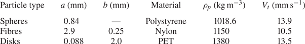
Table 2. Properties of the non-spherical particle types used in the experiment compared with the sphere properties:  $a$, the mean length of the particle axis of rotational symmetry; $b$, the mean length of the other two axes; the particle material; $\rho _p$, the material density; and $V_t$, the terminal velocity.
The terminal velocity  $V_t$ of the disks and fibres is measured by dropping individual particles from rest in a large tank of quiescent water and recording 60 fps videos. Particles are tracked using the same threshold-based method used for the particle sizing (see § 2.4). The tank is deep enough (0.3 m) for the particles to reach terminal velocity before reaching the bottom. The nominal particle Reynolds number is then computed based on the terminal velocity, $\mbox { {Re}}_{p,V_t} = \rho _fV_tD_{p,eq}/\mu$, where $\rho _f$ and $\mu = \rho _f\nu$ are the water density and dynamic viscosity, respectively, and $D_{p,eq}$ is the particle's equivalent diameter, that is, the diameter of a sphere with the same volume as the disk or fibre.
To quantify particle inertia, we refer to the Stokes number. The particle response time is characterised by the time scale with which the particle exponentially approaches the steady-state velocity of the surrounding fluid. For a sphere in creeping flow, this is  $\tau _p=\rho _pD_p^2/18\mu$, which we correct with the Schiller and Naumann expression to account for the finite particle Reynolds number (Clift, Grace & Weber Reference Clift, Grace and Weber2005). In the case of anisotropic particles, the estimation is more complex. An expression for the response time of prolate spheroids is given by Shapiro & Goldenberg (Reference Shapiro and Goldenberg1993)
 \begin{equation}
\tau_p=\frac{2}{9}\frac{\rho_p(b/2)^2}{\mu}\frac{\lambda
\mathrm{ln}(\lambda+(\lambda^2-1)^{1/2})}{(\lambda^2-1)^{1/2}}
. \end{equation}
\begin{equation}
\tau_p=\frac{2}{9}\frac{\rho_p(b/2)^2}{\mu}\frac{\lambda
\mathrm{ln}(\lambda+(\lambda^2-1)^{1/2})}{(\lambda^2-1)^{1/2}}
. \end{equation}
For oblate spheroids, the response time is given by
 \begin{equation}
\tau_p=\frac{2}{9}\frac{\rho_p(b/2)^2}{\mu}\frac{\lambda
[{\rm \pi}-2\tan^{{-}1}(\lambda(1-\lambda^2)^{{-}1/2})]}{2(\lambda^2-1)^{{-}1/2}}
\end{equation}
\begin{equation}
\tau_p=\frac{2}{9}\frac{\rho_p(b/2)^2}{\mu}\frac{\lambda
[{\rm \pi}-2\tan^{{-}1}(\lambda(1-\lambda^2)^{{-}1/2})]}{2(\lambda^2-1)^{{-}1/2}}
\end{equation}
(Zhao et al. Reference Zhao, Challabotla, Andersson and Variano2015). Both of these formulae are derived for particles with an isotropic orientation distribution; this is generally not the case in anisotropic shear flows, thus these formulae are considered a nominal estimate.
For the fluid phase, both the viscous time scale  $\tau ^+$ and the Kolmogorov time scale $\tau _\eta$ are relevant. Here $\tau ^+$ is calculated from the shear velocity $u_\tau$ as $\tau ^+=\nu /u_\tau ^2$, from which we define $\mbox { {St}}^+=\tau _p/\tau ^+$ (the superscript + denoting normalisation by wall units). $\tau _\eta$ varies with the wall normal distance and is estimated from the production–dissipation balance in the turbulent boundary layer (Pope Reference Pope2000). This gives a range for the Stokes number, $\mbox { {St}}_\eta =\tau _p/\tau _\eta$, and for the ratio of particle major axis length to Kolmogorov length, $D_p/\eta$, which are both reported in figure 1.

Figure 1. Wall-normal profiles of (a) the particle Stokes numbers based on the Kolmogorov scale and (b) the particle major axis lengths normalised by the Kolmogorov scale.
The volume fraction of the particles in the system is approximately  $10^{-4}$. The near-wall volume fraction is higher than the mean due to gravitational settling, but remains well below $10^{-3}$. Thus, at the present particle-to-fluid density ratio, the momentum two-way coupling effects are expected to be localised and have a minimal effect on the fluid statistics (Baker & Coletti Reference Baker and Coletti2021; Brandt & Coletti Reference Brandt and Coletti2022). The physical properties of the particles are summarised in table 3. We note that $V_t/u_\tau \sim O(1)$, thus we expect significant gravity effects. This is unlike previous experiments in non-spherical particles in wall turbulence, for which this ratio was at least one order of magnitude smaller (e.g. Shaik et al. Reference Shaik, Kuperman, Rinsky and van Hout2020). Because the key parameters $V_t/u_\tau$ and $\mbox { {St}}^+$ have similar values for the three particle types, the comparison will highlight the influence of their shape. For completeness, we also list the Rouse number $\mbox { {Ro}} = V_t/(\kappa u_\tau )$, which is used in § 3.5.
Table 3. Properties of the particles. Here  $D_p^+$ is the mean particle major axis length in viscous units, $\lambda$ is the aspect ratio, $\rho _p/\rho _f$ is the particle-to-fluid density ratio, $V_t$ is the terminal velocity in still water, $\mbox { {Re}}_{p,V_t}$ is the Reynolds number based on $V_t$ and the particle equivalent diameter, $\mbox { {St}}^+$ is the particle Stokes number based on the viscous time scale of the flow, and $\mbox { {Ro}}=V_t/(\kappa u_\tau )$ is the Rouse number.

2.3. Flow imaging
Time-resolved, planar particle image velocimetry (PIV) is used to measure the velocity of the fluid. The data collection, image processing routine and PIV procedure are described in Baker & Coletti (Reference Baker and Coletti2021), and the only key points are summarised here. The water is seeded with  $13\,\mathrm {\mu }{\rm m}$ silver-coated glass bubbles to act as tracers. A 300 W near-infrared pulsed laser creates a 1 mm light sheet perpendicular to the bottom wall and parallel to the streamwise direction along the channel symmetry plane. Images are captured with a high-speed, 4-megapixel CMOS camera viewing through one of the side walls. For optimal tracking, a frame rate of 500 Hz is chosen to obtain typical displacements of approximately 20 pixels. The recording time amounts to approximately 1900 boundary-layer turnover times.
To obtain fluid velocity fields, the inertial particles are first substituted with Gaussian noise having the same mean and standard deviation as the background image. The resulting tracer-only images are used for PIV processing performed with a custom-written software. Multi-pass cross-correlation with an overlap of 75 % between interrogation windows is used to compute fluid displacement fields. Initial, intermediate and final interrogation window sizes of  $128^2$, $64^2$ and $32^2$ pixels are used, respectively. A signal-to-noise ratio criterion and a universal outlier detection (Westerweel & Scarano Reference Westerweel and Scarano2005) are used to reject spurious velocity vectors. The imaging and PIV processing parameters are summarised in table 4.
Table 4. Imaging and PIV processing parameters:  $f_s$ is the imaging frequency; $N$ is the number of images; $w$ and $h$ are the field of view width and height, respectively; $w_i$ is the final-pass PIV interrogation window size; and $\delta x$ is the PIV vector spacing.
2.4. Particle detection and tracking
We perform particle tracking velocimetry (PTV) on the same images, using different methods to detect the different particle types. The method for detecting the spherical particles is described in Baker & Coletti (Reference Baker and Coletti2021) and is not repeated here. Disk and fibre detection is achieved by an image segmentation method based the particles’ intensity (figure 2). First, a low-pass median filter with a width of 9 pixels is applied to the original images to remove the tracers. Then, images are segmented into inertial particles and background based on an intensity threshold, allowing to locate their centroids. Because the particles have strong contrast with the background, the detection is not sensitive to the exact value of the intensity threshold.

Figure 2. Intensity-based segmentation method for particle detection for (a)–(c) a fibre and (d)–(f) a disk particle: (a), (d) original image, (b), (e) median-filtered image and (c), (f) binarised image, with the red cross indicating the detected particle centroid.
Once the particle centroids are obtained, the particles are tracked between frames (see Baker & Coletti Reference Baker and Coletti2021). Approximately 2500 particles are tracked for each particle type. To obtain particle velocities and accelerations, the particle trajectories are convolved with the first and second derivative of a Gaussian kernel, respectively (Tropea, Yarin & Foss Reference Tropea, Yarin and Foss2007; Voth et al. Reference Voth, La Porta, Crawford, Alexander and Bodenschatz2002; Mordant, Crawford & Bodenschatz Reference Mordant, Crawford and Bodenschatz2004; Gerashchenko et al. Reference Gerashchenko, Sharp, Neuscamman and Warhaft2008; Nemes et al. Reference Nemes, Dasari, Hong, Guala and Coletti2017; Ebrahimian, Sanders & Ghaemi Reference Ebrahimian, Sanders and Ghaemi2019). The optimal width of the kernel  $t_k$ is determined from the variance of the particle acceleration magnitude in the data set. The latter is calculated for a range of kernel widths, and it decays exponentially with kernel width when filtering physical accelerations but decays much faster than exponentially when filtering noise. Therefore, the smallest value for which the variance decays exponentially with kernel width is adopted so that most of the noise is filtered out but most of the physical accelerations are not. This corresponds to a duration of 17 successive snapshots, or approximately $15\tau ^+$ (1–2 $\tau _p$).
In the data analysis, we also consider the fluid velocity at the particle location,  $u_{f|p}$. This is obtained by averaging the fluid velocity vectors within a distance of $D_p/4$ from the edge of particle. As the particles have finite size, this definition does not accurately represent an undisturbed fluid velocity at the particle location (as used in the correct definition of the drag force, Horwitz & Mani Reference Horwitz and Mani2016), but it will serve the purpose of investigating the fluid flow experienced by the particles. The reported results are not affected significantly by the exact value of such distance in the range $D_p/8 - D_p$.
2.5. Particle orientation and rotation measurement
The three-dimensional particle orientation vector,  ${\boldsymbol {p}}$, is evaluated with a projection-based approach. A high spatial resolution of the present imaging system contributes to the successful application of the method, compared with previous studies that determined the in-plane projected orientation from a single-camera view: for example, the full length of an imaged fibre is approximately 80 pixels, comparable to 80 pixels in Metzger et al. (Reference Metzger, Butler and Guazzelli2007) and greater than 64 pixels in Hoseini et al. (Reference Hoseini, Lundell and Andersson2015) and 20 pixels in Dearing et al. (Reference Dearing, Campolo, Capone and Soldati2013) and Carlsson et al. (Reference Carlsson, Håkansson, Kvick, Lundell and Söderberg2011).
The vector  ${\boldsymbol {p}}$ is defined as the unit vector passing through the particle's axis of symmetry, and each component of ${\boldsymbol {p}}$ is the cosine of the angle between this axis and the respective coordinate axis in the water channel reference frame (figure 3). With the caveat that the sign of $p_z$ cannot be determined, the particle orientation can be reconstructed from the apparent pitch ( $\theta$, $\theta '$) and apparent major axis length ( $d$) of the fibre and disk projections, respectively, illustrated in figure 4.

Figure 3. Definition of the particle orientation vector  ${\boldsymbol {p}}$ and its components shown for (a) fibres and (b) disks relative to the water channel reference frame shown in blue.

Figure 4. Diagram defining (a) the apparent pitch  $\theta$ and apparent length $d$ of a fibre and (b) the pitch $\theta '$ and apparent diameter $d$ of a disk.
Before the orientation can be calculated, the apparent major axis length must be corrected for the finite thickness of the particles. The thickness is seen by the camera and artificially increases the apparent major axis length when a particle is seen at an angle (figure 5a). This results in a finite minimum value of  $d$ being measured even when the particle is seen perfectly edge-on. This minimum is taken to be the first-percentile apparent major axis length; that is, the value of $d$ below which 1 % of the observations are found (denoted $d_{1\,\%}$). However, more of the particle thickness is seen as a particle tilts closer to an ‘edge-on’ orientation, so the correction value that must be subtracted depends on the orientation itself. The correction value is scaled linearly with the apparent major axis length, so that the corrected major axis length is given by $d_{corr}=d-d_{1\,\%}(({D_p-d})/{D_p})$. If the resulting shifted major axis length is negative, it is set to zero. The probability density functions (p.d.f.s) of the original $d$ and corrected $d_{corr}$ are shown in figures 5(b) (fibres) and 5(c) (disks).

Figure 5. (a) Schematic of the finite particle thickness when a particle is seen at an angle. The edge of the particle is shown in blue (thickness exaggerated), illustrating how the edge becomes more visible as the particle tilts from a ‘face-on’ to an ‘edge-on’ view. (b), (c) P.d.f.s of the original and corrected apparent major axis length  $d$ and $d_{corr}$, respectively, for (b) fibres and (c) disks.
The set of formulae to compute the correction to the apparent major axis length and the components of the particle orientation vector are given in table 5. Once calculated, the components of  ${\boldsymbol {p}}$ are convolved with a Gaussian smoothing kernel of width 17 frames (the same as was done to obtain particle linear velocity and acceleration) to reduce measurement noise. The unit length of ${\boldsymbol {p}}$ is then checked. If $|1-|{\boldsymbol {p}}||>0.05$, then that orientation observation is rejected and not considered when computing statistics (however, the particle position and velocity values are preserved). This criterion results in the rejection of approximately 1.5 % of fibre and disk observations. Finally, due to the spread in lengths of the fibres, $|p_z|$ will be imaginary if $d_{corr} > D_p$. All three components of ${\boldsymbol {p}}$ are rejected if $|p_z|$ is imaginary, removing approximately 6 % of fibre particle observations.
Table 5. Formulae to compute the particle orientation vector for fibres and disks, as well as the range of each component.

Particle angular velocity and angular acceleration are also of interest. A particle's solid-body rotation rate  $\boldsymbol {\varOmega }$ can be decomposed into a spinning component and a tumbling component, $\boldsymbol {\varOmega }=\varOmega _p{\boldsymbol {p}} + {\boldsymbol {p}}\times \dot {{\boldsymbol {p}}}$, where spinning is rotation about the symmetry axis ( $\varOmega _p{\boldsymbol {p}}$) and tumbling is rotation of the symmetry axis ( ${\boldsymbol {p}}\times \dot {{\boldsymbol {p}}}$). Spinning motion is inaccessible to our optical imaging; we therefore focus on tumbling rates exclusively. The tumbling rate is then given by $\boldsymbol {\omega }_t={\boldsymbol {p}}\times \dot {{\boldsymbol {p}}}$, and the tumbling component of angular acceleration is given by $\boldsymbol {\alpha }_t={\boldsymbol {p}}\times \ddot {{\boldsymbol {p}}}$. The first and second time derivatives of particle orientation, $\dot {{\boldsymbol {p}}}$ and $\ddot {{\boldsymbol {p}}}$, are computed again by convolving the components of ${\boldsymbol {p}}$ with first and second derivatives, respectively, of a Gaussian smoothing kernel of width 17 frames.
Before  $\dot {{\boldsymbol {p}}}$ and $\ddot {{\boldsymbol {p}}}$ are computed, and before ${\boldsymbol {p}}$ is smoothed, ambiguities on the signs of the components of ${\boldsymbol {p}}$ must be resolved in order to ensure that ${\boldsymbol {p}}$ is differentiable. Sign ambiguities occur when the components of ${\boldsymbol {p}}$ reach the bounds of their range. For example, because the range of $p_y$ is $[-1, 1]$, a particle which is tumbling end-over-end in the $x$–
$x$– $y$ plane will eventually reach $p_y \approx -1$ as it passes through the vertical orientation and jump to $p_y \approx 1$ in the next realisation, whereas the value of $p_x$ remains positive throughout. In order to differentiate ${\boldsymbol {p}}$, the signs of $p_y$ and $p_x$ must be flipped as the particle passes through this orientation. Sign ambiguities are resolved by enforcing a minimum angular acceleration condition on the raw (unsmoothed) ${\boldsymbol {p}}$ values. First, observations where any of the components of ${\boldsymbol {p}}$ change sign or approach 0, 1 or $-1$, and are also a local temporal minimum or maximum, are flagged. Three sets of sign changes are applied to the flagged observations: (1) flip only $p_x$ and $p_y$, (2) flip only $p_z$ and (3) flip $p_x$, $p_y$ and $p_z$. The unsmoothed tumbling angular acceleration magnitude $\ddot {{\boldsymbol {p}}}\boldsymbol {\cdot }\ddot {{\boldsymbol {p}}}$ is computed for each case, as well as the original case where no signs are changed. The case with the minimum $\ddot {{\boldsymbol {p}}}\boldsymbol {\cdot }\ddot {{\boldsymbol {p}}}$ is chosen, and the sign change is propagated forward in time along the remainder of that particle's trajectory. In general, the $\ddot {{\boldsymbol {p}}}\boldsymbol {\cdot }\ddot {{\boldsymbol {p}}}$ value associated with the correct set of sign changes will be at least an order of magnitude lower than the other three, so the choice is trivial. Example reconstructed trajectories for a fibre and a disk are shown in figure 6. Notice the tendency of the disks to oscillate about a fairly flat orientation, whereas the fibre orientation is much more variable. These examples are representative of qualitative trends that are illustrated later.

Figure 6. Reconstructed particle trajectories demonstrating typical particle behaviours. Disks to oscillate about a fairly flat orientation, whereas the fibre orientation is much more variable. These examples are representative of qualitative trends that will be illustrated later. Snapshots are shown every five frames ( $3.6\tau ^+$).
2.6. Measurement uncertainty
Uncertainty in the particle statistics is estimated by considering both statistical random uncertainty (due to the finite sample size) and measurement error (due to imperfect centroid and orientation detections). The random uncertainty is estimated by computing 95 % confidence intervals on the statistics (Bendat & Piersol Reference Bendat and Piersol2011). To evaluate the random uncertainty of particle statistics, we assume a number of independent realisations equal to the number of recorded observations in each wall-normal layer (bin) divided by the integral time scale of particle velocity in units of frames. When statistics are computed within wall-normal bins, we assume a number of independent realisations equal to the number of trajectories in each bin.
The measurement error is estimated using synthetic particle templates created from actual particle images. Sphere templates are generated from a sphere image in which one quadrant of the image is mirrored over the horizontal and vertical axes, creating a synthetic particle template for which the centroid is known precisely. Fibre and disk templates are generated from images that are stretched so that  $d = D_p$, then mirrored over each axis as for the spheres. The synthetic particle templates are translated and superimposed upon a tracer-filled background to create synthetic particle trajectories with known centroids. The imposed centroids are chosen to be sinusoids so that the measured derivatives of position and orientation can be compared with their analytical values. A time-series of 3D fibre and disk orientations are defined in which all components of ${\boldsymbol {p}}$ vary sinusoidally. These orientations are projected onto the plane of the image, and particle templates are stretched and rotated according to the projections to simulate what the camera would capture. This allows for both error estimation and validation of the orientation reconstruction algorithm. Then, detection, tracking, and (for disks and fibres) orientation measurements are performed on the synthetic images. The associated uncertainties on the centroid location, velocity, acceleration, orientation, tumbling rate and tumbling acceleration are estimated as the root-mean-square (r.m.s.) difference between measured and actual values. These measurement errors $w_i$ are reported in table 6.
Table 6. Measurement error on the particle centroid location, velocity, acceleration, orientation, tumbling rate and tumbling acceleration for each particle type in SI units, wall units and as a percentage of characteristic values of the quantities.

Uncertainty on the fluid velocities consists of random error and PIV bias error; the random error is dominant. Following Adrian & Westerweel (Reference Adrian and Westerweel2011), the bias error on the PIV correlation peak is estimated as 0.1 pixels, or  $2\,{\rm mm}\,{\rm s}^{-1}$ ( $0.1u_\tau$). To calculate the random uncertainty on statistics, the number of independent samples in the fluid velocity data is estimated as the number of temporally independent realisations (i.e. the number of boundary layer turnover times in the recording) multiplied by the number of spatially independent samples in each realisation (i.e. $w/\delta _{99}$, where $\delta _{99}$ is the boundary layer thickness).
For the fluid velocity evaluated at the particle location, the interpolation also contributes to the uncertainty. This uncertainty is estimated by applying a synthetic particle mask to images where the actual velocity vectors are known, performing PIV analysis on the masked images, then interpolating the resulting fluid velocity at the location of the synthetic particles. The actual fluid velocity is then compared with the interpolated values. The resulting interpolation error on the fluid velocity, again defined as the r.m.s. difference between the actual and calculated values, is approximately  $1\,{\rm mm}\,{\rm s}^{-1}$ ( $0.05u_\tau$) for both fibres and disks, significantly smaller than the random error. To avoid cluttering in the plots, in the following error bars are added only where significant.
3. Results and discussion
3.1. Fluid and particle velocity
We first consider the translational statistics of the particles and fluid. Velocities are Reynolds-decomposed into mean and fluctuating components:  $u=\langle u\rangle +u'$ and $v=\langle v\rangle +v'$, where $u$ and $v$ are the streamwise and wall-normal velocity, respectively, angle brackets denote averaging in time and in the streamwise direction and the prime denoting the fluctuating part. Particle velocities are denoted by $u_p$ and $v_p$, and fluid velocities interpolated at particle locations by $u_{f|p}$ and $v_{f|p}$; unconditional fluid velocities have no subscript. Results are presented in wall units with standard normalisations of velocity, length, time and acceleration: $u^+=u/u_\tau$, $y^+=y/\delta _\nu$, $t^+=tu_\tau /\delta _\nu$ and $a^+=au_\tau ^2/\delta _\nu$, respectively, where $\delta _\nu$ is the viscous length scale. Fibre and disk results are compared with those of the spherical particles from Baker & Coletti (Reference Baker and Coletti2021).
Profiles of particle velocity are obtained by defining wall-normal bins and taking the mean of particle velocities within each. Particles are more numerous near the wall and sparser in the outer region, so the bins are logarithmically spaced to equalise the numbers of particles in each, as well as to capture the high shear in the near-wall region. Profiles of streamwise and wall-normal particle and fluid velocities are shown in figure 7. The deviation of the streamwise velocity profiles of the sphere case in the freestream region (figure 7a) is due to its slightly higher freestream velocity. Within the boundary layer, the mean velocities are not drastically different between the particle shapes, confirming point-particle simulation results (Challabotla et al. Reference Challabotla, Zhao and Andersson2015; Njobuenwu & Fairweather Reference Njobuenwu and Fairweather2016). In all cases, particles lag the fluid within the logarithmic layer due to their inertia (Righetti & Romano Reference Righetti and Romano2004). However, streamwise velocity does differ between particle types near the wall, with the disk velocity significantly larger than that of the fibres and spheres. The sharp decay of the vertical (settling) velocity approaching the wall is discussed in § 3.5.

Figure 7. Wall-normal profiles of mean (a) streamwise and (b) wall-normal particle (circles) and fluid (lines) velocity, compared between sphere (black), fibre (red) and disk (blue) particles.
We investigate the particle slip velocity to understand these trends. The total mean slip velocity can be decomposed into two components, as follows:
 \begin{equation} \langle u_p\rangle - \langle u_f\rangle = \langle u_p - u_{f|p}\rangle + \langle u_{f|p}\rangle - \langle u_f\rangle , \end{equation}
where  $\langle u_p - u_{f|p}\rangle$ is the mean of the local slip velocity and $\langle u_{f|p}\rangle - \langle u_f\rangle$ is the apparent slip velocity. The local slip velocity quantifies the actual instantaneous slip that each particle experiences relative to the surrounding fluid; the apparent slip velocity reflects preferential sampling of slower- or faster-than-average fluid (Kiger & Pan Reference Kiger and Pan2002). The streamwise and wall-normal slip velocities are shown in figure 8. Note that fluid velocity, and therefore slip velocity, is not available below $y^+ \approx 11$ due to the limited PIV resolution.

Figure 8. Wall-normal profiles of mean streamwise (a) total, (b) local and (c) apparent slip velocities and mean wall-normal (d) total, (e) apparent and ( f) local slip velocities for spheres (black), fibres (red) and disks (blue).
From the streamwise slip velocity (figures 8a–8c), it is observed that disks and fibres oversample faster-moving fluid regions below  $y^+ \approx 30$ (as evidenced by their positive apparent slip velocity), suggesting that particles accumulate in high-speed streaks. This preferential sampling is stronger for the fibres and disks than for the spheres, whose apparent slip only slightly exceeds zero near the wall. Disks oversample high-speed fluid so strongly that their total slip near the wall is actually positive. Oversampling of high-speed streaks confirms the findings of recent PR-DNS and experimental studies (Do-Quang et al. Reference Do-Quang, Amberg, Brethouwer and Johansson2014; Shaik et al. Reference Shaik, Kuperman, Rinsky and van Hout2020). The local slip velocity for all three particle shapes is negative for the entire channel depth and becomes more negative as particles approach the wall, indicating that the particles lag the surrounding fluid on average. This is consistent with the expected behaviour of inertial particles. Disks and fibres lag the surrounding fluid by a greater amount than the spheres, suggesting that they have a larger effective inertia. This would not contradict the fact that the spheres have a larger nominal $\mbox { {St}}^+$, because $\mbox { {St}}^+$ of the disks and fibres is calculated assuming an isotropic orientation distribution; as we show in § 3.2, the actual orientation distribution is not isotropic.
The wall-normal slip velocity profiles (figures 8d–8f) reveal further differences between the particle shapes. All three particle shapes have negative local slip velocities in the outer region due to gravitational settling, which decay approaching the wall. However, spheres slightly oversample upward-moving fluid on average, as evidenced by the positive apparent slip, but fibres and disks do not show this behaviour: their apparent vertical slip is near-zero throughout the channel depth. This may be attributed to the spheres oversampling low-speed fluid streaks, which are correlated with upward wall-normal fluid velocities in a turbulent boundary layer; while this behaviour is not exhibited by fibres or disks, which in fact appear to oversample high-speed fluid streaks. Although one may then expect the anisotropic particles to also oversample downward sweep events, we recall that the particle-sampled fluid is evaluated in a region of radius  $D_p/4$, which may smooth out the fluctuations.
The Reynolds stresses of the fluid and particles are compared in figure 9. Overall, the Reynolds stresses of the different particle shapes are fairly similar to each other and to the fluid. (We note that the variation between the fluid Reynolds stress profiles of each case is within experimental uncertainty.) This further confirms the results of point-particle simulations that found little dependence of translational statistics on the aspect ratio (Challabotla et al. Reference Challabotla, Zhao and Andersson2015; Njobuenwu & Fairweather Reference Njobuenwu and Fairweather2016). The streamwise normal stress  $\langle u'u'\rangle$ of the particles is smaller than that of the fluid as the wall-normal height drops below the particle size ( $y^+\lesssim 30$), which can be attributed to wall interactions damping particle streamwise velocities. However, the greatest differences show up in the profiles of $\langle u' v'\rangle$: the shape of the profile for the fibres is similar to that of the spheres, but the magnitude is lower, following the shear stress of the fluid very closely. The increased particle stresses of the spheres was attributed to the effect of particle trajectories crossing fluid streamlines due to the particle inertia (Baker & Coletti Reference Baker and Coletti2021). That the stress profiles of the fibres largely match the shape of the spheres, but are lower in magnitude, may reflect reduced streamline crossing effects and, therefore, a lower effective inertia of the fibres. For the disks, the shape of the profile itself deviates: the shear stress is lower near the wall, and the peak is shifted higher in the boundary layer than either the fibres or spheres, suggesting a somewhat different interaction with the fluid turbulence, as discussed in the next section.

Figure 9. Wall-normal profiles of (a) streamwise, (b) wall-normal and (c) shear stresses for particles (circles) and fluid (lines).
3.2. Particle orientation and tumbling
We next examine the distribution of particle orientations. P.d.f.s of each component of the particle orientation vector,  $p_x$, $p_y$ and $|p_z|$, are shown in figure 10, separated by particle wall-normal position into two bins with $y_p^+ < 100$ and $y_p^+ > 100$. This cutoff was chosen as the point at which roughly half the particles are above this elevation and half are below. For the near-wall set of particles, fibres tend to align their symmetry axis ${\boldsymbol {p}}$ with the streamwise direction (as signaled by the high probability of $p_x$ being close to unity), whereas disks align ${\boldsymbol {p}}$ with the vertical axis (indicated by the absolute values of $p_y$ being often close to unity). Both particle types have some level of preferential alignment with the spanwise axis as well, as indicated by preferential values of $|p_z| > 0$. Disks show a preference towards $p_y$ slightly greater than $-1$ and fibres towards $p_y$ slightly greater than 0. The asymmetry in the p.d.f.s corresponds to a statistical asymmetry in the particle orientations: particles adopt a slightly ‘nose-up’ configuration, as illustrated in figure 11, with their leading edges at a higher elevation than their trailing edges. Far from the wall ( $y_p^+ > 100$), fibres exhibit a much weaker alignment with the streamwise direction and a stronger alignment with the vertical and spanwise directions, indicating a more isotropic orientation. In contrast, disks in the outer region strongly align their symmetry axis with the vertical, corresponding to an approximately flat and level orientation. The streamwise alignment of the fibres and their ‘return to isotropy’ in the outer region agrees with the results of several point-particle simulations (Zhao et al. Reference Zhao, Challabotla, Andersson and Variano2015; Yuan et al. Reference Yuan, Andersson, Zhao, Challabotla and Deng2017; Zhao et al. Reference Zhao, Challabotla, Andersson and Variano2019). However, the alignment of the disks differs from what is found in the point-particle simulations of Challabotla et al. (Reference Challabotla, Zhao and Andersson2015) and Zhao et al. (Reference Zhao, Challabotla, Andersson and Variano2015), which found that inertial disk particles preferentially align with the spanwise axis near the wall. This may be due to the larger spatial extent of the disks and their 2D, rather than 1D shape, making them more difficult to model as point particles compared to fibres. In addition, these point-particle DNS studies neglected gravity, which is an important factor in the dynamics of the large particles considered here.

Figure 10. P.d.f.s of particle orientation components (a)  $p_x$, (b) $p_y$ and (c) $|p_z|$ for fibres (red) and disks (blue) with $y_p^+ < 100$ (circles) and $y_p^+ > 100$ (crosses).

Figure 11. Preferential orientations of (a) fibres and (b) disks near the wall.
P.d.f.s of the squared tumbling rate  $\dot {{\boldsymbol {p}}}\boldsymbol {\cdot }\dot {{\boldsymbol {p}}}$ and squared tumbling acceleration $\ddot {{\boldsymbol {p}}}\boldsymbol {\cdot }\ddot {{\boldsymbol {p}}}$ are compared between particle types for near-wall and outer-region particles in figure 12. The distributions of both $\dot {{\boldsymbol {p}}}\boldsymbol {\cdot }\dot {{\boldsymbol {p}}}$ and $\ddot {{\boldsymbol {p}}}\boldsymbol {\cdot }\ddot {{\boldsymbol {p}}}$ have very long tails, reflecting the high intermittency of tumbling events. Fibres are found to have higher frequencies of extreme $\dot {{\boldsymbol {p}}}\boldsymbol {\cdot }\dot {{\boldsymbol {p}}}$ events than disks near the wall, but no difference is observed between fibres and disks for $\ddot {{\boldsymbol {p}}}\boldsymbol {\cdot }\ddot {{\boldsymbol {p}}}$ or particles far from the wall.

Figure 12. P.d.f.s of (a) particle squared tumbling rate and (b) squared tumbling acceleration for fibres (red) and disks (blue) with  $y_p^+ < 100$ (circles) and $y_p^+ > 100$ (crosses).
Mean profiles of the squared tumbling rate  $\dot {{\boldsymbol {p}}}\boldsymbol {\cdot }\dot {{\boldsymbol {p}}}$ and squared tumbling acceleration $\ddot {{\boldsymbol {p}}}\boldsymbol {\cdot }\ddot {{\boldsymbol {p}}}$ as a function of wall-normal distance are plotted in figure 13. In the outer region of the channel, the profiles are nearly the same for disks and fibres. However, their behaviours diverge below $y^+ \sim 100$. The squared tumbling rate and squared tumbling acceleration for disks peak around $y^+ \sim 40$, below which both quantities drop off and approach zero. In contrast, fibres are much more mobile: their squared tumbling rate and acceleration are much larger than that of disks in the immediate vicinity of the wall. This may suggest that higher inertia of the disks inhibits their tumbling relative to the fibres; it is also likely related to their respective preferential orientations. We investigate possible explanations for this behavior in the following discussion.

Figure 13. Wall-normal profiles of (a) mean squared tumbling rate and (b) mean square tumbling acceleration for fibres (red) and disks (blue).
Further insight can be gained by separating the tumbling rate by component. Figure 14 shows mean profiles of  $\omega _{t,z}$ and r.m.s. profiles of all three tumbling rate components. Fibres have a greater negative $\langle \omega _{t,z}\rangle$ (matching the sense of the mean shear) than disks, which contributes to their larger squared tumbling rate. The r.m.s. tumbling rate provides a better measure of the magnitude of the other two components, because their mean is zero due to the spanwise symmetry of the channel. Fibres have high r.m.s. values of $\omega _{t,y}$ in the inner region, which also contributes to their squared tumbling rate, especially very close to the wall. The higher r.m.s. $\omega _{t,y}$ for fibres compared with that of disks is likely related to their preferential orientations (figure 11), in which rotation about $y$ would be tumbling for fibres but spinning for disks.

Figure 14. Wall-normal profiles of (a) mean  $\omega _{t,z}$ and (b)–(d) r.m.s. tumbling rates of all three components for fibres (red) and disks (blue).
On the other hand, all components of disk tumbling rates approach zero near the wall. Disks approaching the wall tend to stay flat, as seen in the previous section, and do not tumble as much as the fibres. This could be due to their higher moment of inertia, as well as their larger surface area over which turbulent fluctuations are averaged out, making them less responsive to high-frequency intermittent motions that would result in strong tumbling near the wall. However, disks do have higher r.m.s. tumbling about the streamwise axis ( $\omega _{t,x}$) than fibres.
Furthermore, the excess tumbling rate of the fibres compared with the disks is mainly observed in ascending fibres, as shown in figure 15, which compares the mean squared tumbling rates of particles with  $v_p < 0$ and $v_p > 0$. Although ascending and descending disks have similar tumbling rates, the squared tumbling rate of the ascending fibres is much larger than that of the descending fibres near the wall. This implies that the same turbulence events which resuspend fibres also causes them to tumble strongly.

Figure 15. Wall-normal profiles of mean squared tumbling rate for ascending and descending fibres (red) and disks (blue). Ascending particles are shown in circles and descending particles are shown in crosses.
We now consider the temporal coherence of the particle orientation and tumbling using Lagrangian autocorrelations. These are calculated as follows (for the generic particle quantity  $q_p$):
 \begin{equation} \rho_{q_p}(\Delta t,
y_0) = \frac{\langle q_p'(t_0, y_0) q_p'(t_0 + \Delta
t, y_0)\rangle}{\langle q_p'(t_0,
y_0)^2\rangle^{1/2} \langle q_p'(t_0 + \Delta t,
y_0)^2\rangle^{1/2}} .
\end{equation}
\begin{equation} \rho_{q_p}(\Delta t,
y_0) = \frac{\langle q_p'(t_0, y_0) q_p'(t_0 + \Delta
t, y_0)\rangle}{\langle q_p'(t_0,
y_0)^2\rangle^{1/2} \langle q_p'(t_0 + \Delta t,
y_0)^2\rangle^{1/2}} .
\end{equation}
The subscript 0 denotes the origin of a trajectory, so that  $t_0$ and $y_0$ are the initial time and wall-normal location of each trajectory, respectively. Here the fluctuating component of the quantity, $q_p'$, is determined by subtracting from each trajectory the Lagrangian mean calculated along each trajectory $\langle q_p(\Delta t, y_0)\rangle _L$:
 \begin{equation} q_p'(t_0+\Delta t, y_0) = q_p(t_0+\Delta t, y_0) - \left\langle q_p(\Delta t, y_0)\right\rangle_L . \end{equation}
Autocorrelations are calculated within four logarithmically spaced wall-normal bins to capture trends in different parts of the boundary layer. Figure 16 shows results for  $p_x$ and $p_y$, indicating that a wide range of correlation time scales exists. For near-wall and log-layer locations, the particle orientations are correlated over times of the order of the boundary layer turnover time ( $\sim 30\tau ^+$), indicating that the dynamics are governed by the energetic eddies. In the outer region, the correlation times are even longer, as expected because of the small mean shear and rare occurrence of high-vorticity events at those heights. Moreover, there are strong differences between the particle types. The fibres are much more sensitive to wall-normal distance than the disks, with a wide spread between the curves close to and far from the wall for fibres and a much smaller spread for disks. This confirms that fibres are more responsive to intermittent small-scale turbulent events occurring near the wall that induce tumbling. For $p_y$, in particular, disks show a remarkable amount of temporal coherence, with very slowly decaying autocorrelations. This translates into relatively stable disk orientations across the channel depth in flat and level or slightly tilted configurations, whereas fibres display stability in the freestream region but have more variable orientations nearer to the wall. As we argue in the next sub-section, the physical explanation is to be found in the effective response time of the particles, which (despite the similar nominal value) is effectively larger for the disks than for the fibres. This also supports the findings of Marchioli et al. (Reference Marchioli, Fantoni and Soldati2010) that prolate particles have a preferred streamwise orientation, but this orientation is unstable near the wall due to the wall-normal velocity gradient.

Figure 16. Lagrangian autocorrelations of (a), (b)  $p_x$ and (c), (d) $p_y$ for (a), (c) fibres and (b), (d) disks calculated within four wall-normal bins.
We then turn to the autocorrelations of spanwise tumbling rate  $\omega _{t,z}$ (figure 17) to investigate the temporal coherence of tumbling motion. In the near-wall region, these decay over times of the order of the nominal response times of the particles $\tau _p \sim O(10\tau ^+)$, consistent with the notion that the rotational and translational response times of anisotropic particles are of the same order (Voth & Soldati Reference Voth and Soldati2017). The autocorrelations for the disks decay faster than those of the fibres at all wall-normal distances, which is opposite to the trend found for $p_y$. Taken together along with the mean and r.m.s. tumbling rates (figure 14), this suggests two different modes of motion undergone by disks and fibres. Disks tend to wobble about their preferential orientation, which causes their tumbling rate to vary over short time scales while their $p_y$ is coherent. In contrast, fibres tumble end-over-end, resulting in less coherent $p_y$ and more coherent $\omega _{t,z}$. That the $\omega _{t,z}$ autocorrelations decay faster at lower $y^+$ implies that turbulence is an important driver of both disks’ and fibres’ tumbling motion.

Figure 17. Lagrangian autocorrelations of  $\omega _{t,z}$ for (a) fibres and (b) disks calculated within four wall-normal bins.
These tendencies are illustrated with the example particle trajectories in figure 6. Fibres (figures 6a–6d) are unstable and tumble freely. Their tumbling is mostly about the  $z$ (spanwise) and $y$ (wall-normal) axes, resulting in a tilted ‘pole-vaulting’ or ‘kayaking’ mode of rotation. Disks (figures 6e–6h) are much more stable and strongly prefer a nearly flat orientation. They wobble from side to side about this orientation, producing highly variable tumbling about the $x$ (streamwise) axis. For both particle shapes, tumbling is more intense within the log layer.
3.3. Acceleration and hydrodynamic response
We next address the question of shape effects on the particle hydrodynamic response, considering the particle translational and rotational acceleration. Wall-normal profiles of mean and r.m.s. accelerations in the streamwise and wall-normal directions are shown in figure 18. No significant difference is observed in the mean acceleration profiles between particle shapes: near the wall, particles tend to have negative  $\langle a_{x,p}\rangle$ as they fall into slower fluid (Baker & Coletti Reference Baker and Coletti2021), being occasionally slowed further down by direct contact with the wall (see § 3.4); while the positive $\langle a_{y,p}\rangle$ near the wall is attributed to both turbulent resuspension and, at low $y^+$, hindered settling as particles approach the wall. On the other hand, the r.m.s. accelerations show shape effects. The r.m.s. accelerations for both $x$ and $y$ components are lowest for disks, r.m.s.( $a_{x,p}$) in particular being much lower than for fibres or spheres. In general, the magnitude of particle r.m.s. acceleration tends to decrease with increasing particle inertia for spheres (Volk et al. Reference Volk, Calzavarini, Verhille, Lohse, Mordant, Pinton and Toschi2008, Reference Volk, Calzavarini, Lévêque and Pinton2011); this has also been confirmed for prolate ellipsoids using point-particle DNS (Ouchene et al. Reference Ouchene, Polanco, Vinkovic and Simoëns2018). Thus the present results indicate a significantly larger effective inertia of the disks in the streamwise direction, despite a nominal response time comparable to that of spheres and fibres. Likewise, the fibres have lower r.m.s.( $a_{y,p}$) but similar r.m.s.( $a_{x,p}$) compared with spheres, implying a preferential attenuation of their response to fluid fluctuations depending on their orientation. Overall, the non-monotonic trends in the r.m.s.( $a_{x,p}$) and r.m.s.( $a_{y,p}$) suggest that a scalar Stokes number is not a sufficient descriptor for the response of non-spherical particles to anisotropic turbulent flows.

Figure 18. Wall-normal profiles of (a), (b) mean and (c), (d) r.m.s. particle acceleration for spheres (black), fibres (red) and disks (blue). Streamwise acceleration is shown in crosses and wall-normal acceleration is shown in circles.
The patterns observed in the r.m.s. accelerations are consistent with disks and fibres that preferentially orient with their largest cross-section orientation parallel to the streamwise direction, that is,  $|p_y| \sim 1$ for disks and $|p_x| \sim 1$ for fibres. Particles oriented this way have greater wall-normal drag coefficients than streamwise drag coefficients, which could result in longer translational response times.
We also consider the particle rotational response times. The rotational response time is generally smaller than the translational one, and for non-spherical particles is expected to depend on the different axes of rotation (Zhao et al. Reference Zhao, Challabotla, Andersson and Variano2015). Here we are only able to examine the tumbling components. Analogously to the translational response time, we examine trends using the r.m.s. profiles of particle angular acceleration. The r.m.s. profiles of the three tumbling acceleration components are shown in figure 19. Disks have a larger r.m.s.( $\alpha _{t,x}$), suggesting a shorter response time for tumbling around the streamwise direction, whereas fibres have a larger r.m.s.( $\alpha _{t,y}$), implying a shorter response time for tumbling around the wall-normal direction. The value of r.m.s.( $\alpha _{t,z}$) is similarly small for both particle types. This picture reflects the anisotropic orientation distribution and the tensorial nature of the rotational dynamics. For an accurate description of the latter, one would need to define the response times around each axes. This can, in principle, be obtained from the Lagrangian autocorrelation of the rotational accelerations. However, the latter are very sensitive to noise and require an even higher spatiotemporal precision in the tracking process.

Figure 19. Profiles of the r.m.s. (a)  $x$, (b) $y$ and (c) $z$ components of tumbling acceleration for fibres (red) and disks (blue).
3.4. Wall interactions
One mechanism for particle tumbling near the wall is the direct interaction with the wall itself. Due to the particles’ extended dimensions and finite slip velocity, friction due to direct contact or lubrication (Kundu, Cohen & Dowling Reference Kundu, Cohen and Dowling2012) with the wall could exert significant torques on particles. To isolate the effect of wall contact, we consider particles located within one semimajor axis length from the wall and compare between those that are contacting the wall and those that are not. Wall contact is inferred when the lower edge of a particle coincides with the wall within measurement uncertainty. Although this definition does not necessarily guarantee wall contact, it does capture particles that are close enough to the wall to feel its effects, either through contact or lubrication. Figure 20 shows p.d.f.s of squared tumbling rate (figure 20a) and squared tumbling acceleration (figure 20b), compared between wall-contacting and non-contacting disks and fibres with  $y_p < D_p/2$. A clear excess of extreme tumbling rates and accelerations is observed in the set of particles contacting the wall for both shapes. The fibres see a greater increase in the frequency of extreme tumbling rates and accelerations for wall contact. This is expected since the fibres have much smaller moment of inertia.

Figure 20. P.d.f.s of (a) squared tumbling rate and (b) squared tumbling acceleration for fibres (red) and disks (blue) within  $D_p/2$ from the wall which are not contacting the wall (crosses) and are in contact with the wall (circles).
The above p.d.f.s are then broken down into directional components, and the same sets of particles are compared again to investigate the mechanics of wall-friction tumbling events (figure 21). As expected, extreme tumbling rates and accelerations of several components are more frequent for wall-contacting particles than non-contacting particles. However, the tumbling behaviour about the various axes is non-trivial. Wall-contacting fibres are found to have strong tumbling rates and accelerations more frequently about both the spanwise and wall-normal axes than non-contacting fibres. This implies that wall interactions induce a titled ‘pole-vaulting’ or ‘kayaking’ mode of tumbling in fibres. The  $z$ component of tumbling rate and acceleration is skewed negatively, showing that this motion occurs in the same direction as the rotation due to mean shear. The tilted nature of the rotation may be due to the influence of spanwise shear due to high- and low-speed streaks, as found by Wang et al. (Reference Wang, Abbas, Yu, Pedrono and Climent2018). Disks in contact with the wall, on the other hand, show stronger tumbling about the wall-normal axis, and to a smaller degree the streamwise axis, but not the spanwise axis. This suggests that wall friction does not induce disks to tumble end-over-end, as it does fibres. Instead, the mode of disk tumbling during wall interactions could be described as wobbling and precessing, much like a spinning top. This mode of tumbling is likely to result from the disks ‘nose-up’ preferential orientation, which does not put the disks in a position to have their front edge contact the wall. Their point of contact is much more likely to be on the rear or side edges, which would produce a torque more in line with the $x$ and $y$ axes. These near-wall processes are illustrated in figure 22.

Figure 21. P.d.f.s of (a)–(c) tumbling rate and (d)–(f) tumbling acceleration components for fibres (red) and disks (blue) within  $D_p/2$ of the wall which are not contacting the wall (crosses) and are in contact with the wall (circles).

Figure 22. Example (a), (b) fibre and (c), (d) disk trajectories for particles (a), (c) contacting the wall and (b), (d) with  $y_p < D_p/2$. Particle snapshots are shown every 5 frames ( $3.6\tau ^+$). The corresponding $\omega _{t,z}$ over time for the two fibres are shown in (e) and $\omega _{t,y}$ for the two disk trajectories are shown in ( f).
We also consider the duration of time  $t_{wall}$ for which particles are in continuous contact with the wall. P.d.f.s of $t_{wall}$ are shown for each particle type in figure 23. The p.d.f.s are found to follow an exponential decay of the form $\text {p.d.f.} \propto \exp (t_{wall}/\tau _{wall})$. Here, $\tau _{wall}$ is the time scale characterising the distribution of durations of wall contact. It is also roughly equal to the mean value of $t_{wall}$. For spheres, $\tau _{wall}$ was found to match $\tau _p$ very closely, as discussed in Baker & Coletti (Reference Baker and Coletti2021). For the fibres and disks, $\tau _{wall}$ is still found to be comparable to $\tau _p$ obtained from (2.1) and (2.2), as listed in table 7. The wall-contact time scale is also compared to the particle settling velocity time scale, $\tau _{p,g}=V_t/g$. In table 7, this is found to be much smaller than either $\tau _p$ or $\tau _{wall}$. Here $\tau _{p,g}$ primarily quantifies the particle's settling behaviour, whereas $\tau _p$ mainly correlates with the particle's response to the instantaneous slip relative to the fluid, which as seen in figure 8, is primarily in the streamwise direction. That $\tau _{wall}$ is much closer to $\tau _p$ than $\tau _{p,g}$ suggests that the duration of particle–wall interactions is dominated by the particles’ response to the slip velocity, rather than gravity.

Figure 23. P.d.f.s of the duration of wall interactions for spheres (black), fibres (red) and disks (blue).


3.5. Particle spatial distribution and dispersion
Finally, we explore particle spatial distribution and dispersion. It is common to model the vertical transport of heavy particles in turbulent boundary layers as an idealised process where particles constantly settle at a velocity  $V_t$ while being suspended upward by turbulent fluid motions (Yang Reference Yang1996). An equilibrium is achieved where the concentration is greatest near the wall and drops off with height, so turbulent motions carry more particles upward on average than downward. Thus, the mean particle concentration profile results from a balance between gravitational settling and turbulent resuspension. Under the assumptions that (i) equilibrium conditions are achieved (i.e. fully developed concentration profile and vertical net flux of particles $\varPhi = 0$), (ii) particles settle at their quiescent-fluid terminal velocity $V_t$ and (iii) the vertical turbulent mass flux obeys Fickian diffusion with a particle diffusivity equal to the eddy viscosity ( $\varepsilon _p = \varepsilon _f = \kappa u_\tau y$), this balance is represented by an advection–diffusion equation:
 \begin{equation} \varPhi = \langle C\rangle V_t - \varepsilon_p\frac{\mathrm{d}\langle C\rangle}{\mathrm{d} y}, \end{equation}
where  $C$ is the particle concentration. Integrating, one obtains the well-known concentration profile (Rouse Reference Rouse1939; Prandtl Reference Prandtl1952):
 \begin{equation} \frac{\langle C\rangle}{\langle C\rangle_{ref}} = \left(\frac{y}{y_{ref}}\right)^{{-}Ro}, \end{equation}
where  $y_{ref}$ is an arbitrary reference height (here, $y_{ref}=100^+$), $\langle C\rangle _{ref}$ is the corresponding concentration and the Rouse number $\mbox { {Ro}} = V_t/(\kappa u_\tau$) (reported in table 3 for the present cases) quantifies the relative strength of gravitational settling and turbulent resuspension.
Mean wall-normal profiles of particle concentration are displayed in figure 24, compared with (3.5). The spheres show a large deviation from Rouse–Prandtl theory, which in Baker & Coletti (Reference Baker and Coletti2021) was attributed to their inertia (neglected in the theory) and the near-wall settling velocity  $\langle v_p\rangle$ being smaller than $V_t$. The concentration profiles for fibres and disks are consistent with (3.5) in the range $30 < y^+ < 200$, despite their finite size and inertia; above and below that range, however, the deviation becomes apparent.

Figure 24. Wall-normal profiles of mean particle concentration for spheres (black), fibres (red) and disks (blue) compared with the Rouse–Prandtl theory of (3.5) (lines). Concentration is normalised by its reference value at  $y_p^+ = 100$. Each profile is shifted horizontally by a factor of $10^2$ for clarity.
An in-depth assessment of this theory for inertial spherical particles was carried out in the wind tunnel study of Berk & Coletti (Reference Berk and Coletti2020). The concentration profiles of disks and fibres in the present experiment are similar to those of the intermediate-Ro particles ( $\mbox { {Ro}} \sim 1$) in their study, with a concentration deficit near the wall and an excess in the freestream, whereas the concentration profile of the spheres in the present experiments resembles the higher-Ro particles ( $\mbox { {Ro}} \sim 2$) in Berk & Coletti (Reference Berk and Coletti2020). They argued that these deviations could be explained by the particles’ decreasing settling velocity approaching the wall and by a small but measurable downward flux in the outer region, whereas the assumption of Fickian diffusion with $\varepsilon _p \approx \kappa u_\tau y$ was tenable.
The present data provides a test of the arguments of Berk & Coletti (Reference Berk and Coletti2020) in a very different regime: their experiments, while having similar Ro and St, were performed with glass particles in air, resulting a higher particle-to-fluid density ratio and a much higher flow Reynolds number. We first evaluate the vertical flux and provide estimates of the particle diffusivity. The net flux  $\varPhi$ is computed by counting particles as they cross horizontal planes spaced logarithmically in $y$ (as in Fong, Amili & Coletti Reference Fong, Amili and Coletti2019; Berk & Coletti Reference Berk and Coletti2020), resulting in the profile in figure 25. There is a small negative net flux in the outer region of the flow, as was the case in the experiments of Berk & Coletti (Reference Berk and Coletti2020), whose magnitude is approximately 2 % of the streamwise particle flux for all particle types. This indicates a slight non-equilibrium condition and may explain some of the deviation from Rouse–Prandtl theory in the outer region. The small positive flux of disks near the wall may also contribute to the deviation of the disk concentration from Rouse–Prandtl theory at lower $y^+$.

Figure 25. Wall-normal profiles of the net particle flux for spheres (black), fibres (red) and disks (blue).
We estimate the diffusivity leveraging Taylor theory, which states that the particles’ diffusivity depends on the velocity variance and on the integral timescale of their fluctuating motion (Furbish, Ball & Schmeeckle Reference Furbish, Ball and Schmeeckle2012), here considered along the vertical direction:
 \begin{equation} \varepsilon_p(y) = T_{v_p}\langle v_p'^2\rangle . \end{equation}
The timescale  $T_{v_p}$ can be calculated from the Lagrangian velocity autocorrelation. Due to the limited trajectory lengths, $T_{v_p}$ is taken to be the $e$-folding time of an exponential function fitted to the autocorrelation, as shown in figure 26.

Figure 26. Lagrangian autocorrelations of  $v_p$ for (a) spheres, (b) fibres and (c) disks calculated within the same four wall-normal bins as in figures 16 and 17. Dashed lines indicate an exponential fit to the data.
These diffusivity estimates are compared with two estimates of the eddy viscosity (i.e. the turbulent diffusivity of the fluid momentum): the first from Prandtl theory for a canonical boundary layer (Pope Reference Pope2000):
 \begin{equation} \varepsilon_{f,Pr} =
\left\{\begin{array}{@{}ll} \kappa u_\tau y, & \text{for } y
< 0.2\delta_{99}, \\ 0.09\delta_{99}u_\tau, & \text{for } y
> 0.2\delta_{99} \end{array} \right.
\end{equation}
\begin{equation} \varepsilon_{f,Pr} =
\left\{\begin{array}{@{}ll} \kappa u_\tau y, & \text{for } y
< 0.2\delta_{99}, \\ 0.09\delta_{99}u_\tau, & \text{for } y
> 0.2\delta_{99} \end{array} \right.
\end{equation}
and the second from the eddy-viscosity assumption for the Reynolds shear stress:
 \begin{equation} \varepsilon_{f,\nu_T}=\left|\frac{\langle u'v'\rangle}{\mathrm{d}\langle u\rangle/\mathrm{d}y}\right|. \end{equation}
 The particle and fluid diffusivity profiles are presented in figure 27. Both estimates of  $\varepsilon _{f}$ are remarkably similar for $y^+ \leq 100$, beyond which the discrepancies are attributed to the deficiencies of the eddy-viscosity assumption in presence of vanishingly small shear. $\varepsilon _p$ follows the fluid diffusivity profile remarkably closely. Overall, as in Berk & Coletti (Reference Berk and Coletti2020), we find strong support for the assumption of Fickian diffusion with $\varepsilon _p \approx \kappa u_\tau y$, at least for the regime $\mbox { {St}}^+ \sim O(10)$ and $\mbox { {Ro}} \sim O(1)$.

Figure 27. Wall-normal profiles of estimated fluid and particle diffusivities for spheres (black), fibres (red) and disks (blue). Solid black line corresponds to Prandtl diffusivity, dashed black line to eddy viscosity, crosses to particle diffusivity based on Taylor theory and circles to particle diffusivity based on the particle flux.
We now consider the mean particle wall-normal velocity. Rouse–Prandtl theory assumes that particles settle with a constant velocity  $V_t$ relative to the local fluid velocity. However, as we have already seen in figure 8(e), a strong reduction in settling velocity is observed below $y^+ \approx 200$. Figure 28 displays mean profiles of local vertical slip velocity normalised by $V_t$, and shows that the settling velocity starts to drop off several major axis lengths from the wall. The particle diffusivity profiles in figure 27 provide an immediate explanation for the decrease of the settling velocity: under the present quasi-equilibrium conditions (fully developed turbulent boundary layer and small vertical flux), gravitational settling and turbulent resuspension are in balance, $\langle C\rangle \langle v_p\rangle =\varepsilon _p \,\mathrm {d}\langle C\rangle /\mathrm {d}y$. Rouse–Prandtl theory assumes a constant settling velocity $\langle v_p\rangle =V_t$, which is clearly not tenable, yielding a power-law profile of concentration which tends to infinity at the wall. Vice versa, keeping the concentration finite and letting the vertical velocity vary with $y$, the vanishing turbulent diffusivity (of both momentum and particles) at the wall also implies vanishing gravitational settling. Along with our previous studies (Berk & Coletti Reference Berk and Coletti2020; Baker & Coletti Reference Baker and Coletti2021), the present results corroborate this view for a wide range of particle sizes, shapes, density ratios and Reynolds numbers.

Figure 28. Wall-normal profiles of mean local vertical slip velocity for spheres (black), fibres (red) and disks (blue) normalised by each particle's still-fluid terminal velocity. In addition, horizontal dashed lines show a height of one  $D_p$ from the wall for each particle type in their respective colours.
A further explanation for the near-wall concentration deficit of the fibres and disks may be related to an inherent limitation of Rouse–Prandtl theory (Boudreau & Hill Reference Boudreau and Hill2020). Because it follows a power law, the concentration at the wall is predicted to be infinite. For finite-size spheres, a particle centroid necessarily will not be observed below one particle radius from the wall, hence Rouse–Prandtl theory is invalidated for  $y < D_p/2$. For anisotropic particles, however, the height below which a particle centroid cannot be present depends on the particle orientation. When particles have a range of orientations, a gradual concentration drop-off between one semimajor and one semiminor axis from the wall is expected. In addition to this mechanical constraint, an upward pressure force due to lubrication between the particles and the wall may become significant when the distance is less than one major axis length, which would suppress both the concentration and settling velocity in this region (Kundu et al. Reference Kundu, Cohen and Dowling2012). The lubrication effect would be stronger for disks than fibres due to their larger planar area, which may explain why the near-wall concentration deficit is larger for disks than for fibres.
We note that the simple yet powerful Rouse–Prandtl theory has a long history of successfully predicting concentration profiles of small, dense, compact silt and sediment grains in water flows (Garcia Reference Garcia2008). However, the model may be less well-suited for other particle types. A parametric study considering the effects of  $\mbox { {St}}^+$, Ro, $\rho _p/\rho _f$, $D_p^+$ and $\lambda$ on particle concentration profiles is needed to determine which classes of particles may be well described by this theory.
4. Summary and conclusions
We have performed an experimental study of disks and fibres with  $\mbox { {St}}^+ \sim O(10)$, $\mbox { {Ro}} \sim O(1)$ and $D_p^+ \sim O(50)$, in a water turbulent boundary layer at $\mbox { {Re}}_\tau = 620$. Their translational and rotational (tumbling) behaviour, as well as their concentration and dispersion, have been investigated and compared with those of spherical particles with similar inertia and settling properties. The mean particle velocity and Reynolds stresses are largely similar between spherical and non-spherical particles. Disks and fibres both oversample high-speed fluid regions near the wall. Therefore, despite their significant inertia, they approach or even exceed the mean fluid velocity in the vicinity of the wall.
The analysis of the particle orientation confirms that fibres tend to align mostly in the streamwise direction, whereas disks strongly prefer to align their symmetry axis quasi-normal to the wall, with a nose-up configuration. Tumbling is stronger near the wall than in the outer region for both disks and fibres, reflecting the strong shear and turbulence in that region. Tumbling rates are higher for fibres than for disks, with the excess mostly contributed by fibres which are ascending. Lagrangian autocorrelations of particle orientation indicate that the disks’ preferential orientation is quite stable. On the other hand, the autocorrelations of fibre orientation components decay more quickly, and the decay rate has a strong dependence on wall-normal distance, indicating that shear and turbulence destabilise their orientation.
The particle r.m.s. accelerations differ with particle shape, implying that the fibres respond more quickly to the turbulent fluctuations, while the disks have a slower response in particular to the wall-normal fluctuations. In general, large differences between the r.m.s. accelerations of the various components underscore how a scalar parameter (such as the Stokes number) cannot comprehensively describe the inertia of non-spherical particles in an anisotropic flow. This also applies to rotational inertia, with disks showing lower resistance to tumbling around the streamwise direction, and fibres having lower resistance to tumbling around the wall-normal direction.
Strong tumbling events are found in the set of particles that come in contact with the wall, implicating wall friction as an additional tumbling mechanism. As for spheres, the distribution of particle–wall contact durations follows as exponential distribution with a characteristic timescale comparable to the nominal hydrodynamic response time, and much larger than the response time to gravitational settling. This implies that particle–wall interactions are influenced more by the surrounding flow than by gravity.
The mean concentration profiles of both fibres and disks follow the profile predicted by Rouse–Prandtl theory only in the range  $30 < y^+ < 200$. As recently shown for spheres in both water (Baker & Coletti Reference Baker and Coletti2021) and air (Berk & Coletti Reference Berk and Coletti2020), the deviations above that range are likely due to a small but non-zero wall-normal particle flux in the outer region, and the deviations below that range are mainly due to the rapid decrease of the settling velocity below $y^+ \approx 200$ (down to vanishingly small levels below $y^+ \approx 50$). The latter is attributed to the reduction in the particle diffusivity, which solely balances gravitational settling under equilibrium conditions. Indeed their diffusivity closely follow the fluid momentum diffusivity throughout the boundary layer, thus also vanishing at the wall. Moreover, particle–wall interactions also contribute to reduce the near-wall settling velocity at heights comparable to the particle size.
The present study has focused on specific particle sizes, shapes and flow regime, allowing for an in-depth analysis of the inter-phase interaction. The physical mechanisms that we describe, however, are generally applicable. In particular, taking together the results of this study, comparing them with our previous results (Berk & Coletti Reference Berk and Coletti2020; Baker & Coletti Reference Baker and Coletti2021) and the relevant literature on spherical and non-spherical inertial particles in wall turbulence, we come to the following main conclusions.
(i) The particle streamwise velocity with respect to the fluid varies across the boundary layer. In the quasi-quiescent region adjacent to the free stream, the particles are in equilibrium with the fluid and travel at its same speed; while in the logarithmic region, they are permanently adjusting to the fluid fluctuations and lag the flow with a mean slip velocity of approximately $O(u_\tau )$. Near the wall, the particle relative speed depends on the interactions with the wall; these are especially consequential for disks and fibres, causing them to reside in high-speed streaks and thus to reach or exceed the mean fluid velocity.
(ii) The particle shape has profound influence on the orientation and rotational motion. The fibres have their symmetry axis preferentially aligned with the streamwise direction, whereas the disks have it almost normal to the wall, both of them keeping their ‘nose’ slightly up. The fibres are more sensitive to near-wall turbulence, which cause them to rapidly tumble end-to-end, whereas disks wobble around their average position.
(iii) The duration of the direct wall–particle interactions follow an exponential distribution of order
$\tau _p$. For anisotropic particles, and especially for fibres, such interactions are responsible for strong intermittency in the tumbling rates and tumbling accelerations.(iv) Although one can define a nominal response time for non-spherical particles, their aerodynamic response will depend on the orientation with respect to the flow. Thus, the Stokes number is not sufficient to describe the inertia of finite-size non-spherical particles, which respond differently to turbulent fluctuations based on their shape and along different directions.
(v) The particle diffusivity varies significantly across the boundary layer, being close to the classic scaling for momentum diffusivity
$\sim \kappa u_\tau y$. Equilibrium conditions then imply that the particle settling velocity vanishes approaching the wall. In turn, this leads to large departures from the Rouse–Prandtl predictions of the concentration profile for heavy particles in wall turbulence: such a theory (which neglects particle inertia and assumes constant settling velocity) may overestimate the near wall concentration by one order of magnitude or more.


The present study presents several new insights on the behaviour and dynamics of finite-size non-spherical particles in a turbulent boundary layer. However, additional effort is warranted to gain a more complete picture of the particle–fluid dynamics. For example, high-resolution measurements of the detailed fluid velocity fields surrounding the particles, especially near the wall, are needed to resolve the actual wall contact and further elucidate its role. In addition, the effects of particle size, inertia and aspect ratio may be isolated and explored in future parametric studies. Finally, given the moderate Reynolds number, small density ratio and relatively large particle size, the present regime appears ideal for a one-to-one comparison with PR-DNS.
Funding
This work was funded by the Legislative-Citizen Commission on Minnesota Resources (LCCMR). L.J.B. was supported by the Department of Defense (DoD) through the National Defense Science and Engineering Graduate Fellowship (NDSEGF) Program.
Declaration of interests
The authors report no conflict of interest.


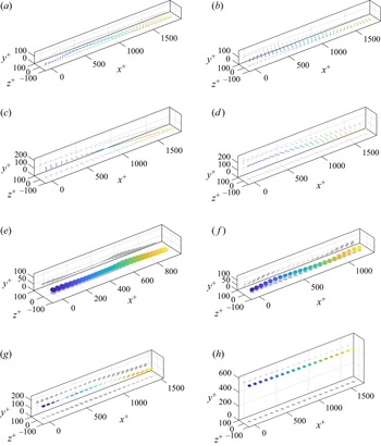


 Open access