


1. Introduction
Bubble motion is widely applied in metallurgical and nuclear industries to enhance the efficiency of stirring (Thomas, Huang & Sussman Reference Thomas, Huang and Sussman1994; Jin, Vanka & Thomas Reference Jin, Vanka and Thomas2018) or heat transfer (Bender & Hoffman Reference Bender and Hoffman1977; Serizawa et al. Reference Serizawa, Ida, Takahashi and Michiyoshi1990; Morley et al. Reference Morley, Smolentsev, Barleon, Kirillov and Takahashi2000) and a magnetic field (MF) offers an approach to control the bubble movement with a contactless method in conductive liquids. In these situations, bubbles are considered to have complex motion characteristics in a liquid metal, and it is of significance to study the bubble motion mechanism with a MF applied. However, the physical properties of liquid metals bring great difficulties to experimental research, and traditional optical methods are almost impossible to apply due to the opacity of liquid metal.
Electrical probes were used by Mori, Hijikata & Kuriyama (Reference Mori, Hijikata and Kuriyama1977) and Eckert, Gerbeth & Lielausis (Reference Eckert, Gerbeth and Lielausis2000a,Reference Eckert, Gerbeth and Lielausisb) to measure the bubble velocity and distribution of the void fraction in a liquid metal. However, as electrical probes must be immersed in a liquid metal, they can influence the bubble motion. With the development of acoustic theory and detection technology, an acoustic method was partially applied to measure the characteristics of liquid metal flow in a contactless way (Andreini, Foster & Callen Reference Andreini, Foster and Callen1977; Ishimoto et al. Reference Ishimoto, Okubo, Kamiyama and Higashitani1995; Schmerr Reference Schmerr2014). Based on the development of ultrasonic Doppler velocimetry (UDV), Zhang, Eckert & Gerbeth (Reference Zhang, Eckert and Gerbeth2005) measured the bubble velocities in a GaInSn alloy with a streamwise MF applied, and it was revealed that the influence of the MF on the bubble velocity is related to the bubble size. When the Eötvös number  $Eo<2.5$, the MF increased the drag coefficient of the bubble, while for those bubbles with $Eo>3.6$ their velocities were greater. The Eötvös number represents the ratio of the buoyancy force to the surface tension, and it is often used to represent the dimensionless size of a bubble. Zhang, Eckert & Gerbeth (Reference Zhang, Eckert and Gerbeth2007) also found an anisotropy of the void fraction obtained by UDV when bubble chains were influenced by a horizontal MF, and the void fraction was much higher in the direction perpendicular to the MF. Then, UDV was applied to measure the argon bubble velocity in GaInSn under a horizontal MF by Wang et al. (Reference Wang, Wang, Meng and Ni2017) and the results indicated that the MF would accelerate the bubble when the magnetic interaction parameter $N<1$ and suppress its rise when $N>1$. This conclusion was also proven in the experimental research by Strumpf (Reference Strumpf2017). The magnetic interaction parameter is the ratio of the electromagnetic force to the inertial force, which is often used in magnetohydrodynamics (MHD) research, such as in the study of Davidson (Reference Davidson2001).
However, it is also difficult for UDV to detect three-dimensional (3-D) bubble motion in a liquid metal as the UDV measures the velocity distribution along the ultrasonic wave direction. Benefitting from the strong penetration ability of high-energy rays, a radiographic technology was also utilized to visualize the bubble trajectories in several liquid metals. Irons & Guthrie (Reference Irons and Guthrie1980) obtained bubble images in an indium-gallium melt using an X-ray system and Gnyloskurenko & Nakamura (Reference Gnyloskurenko and Nakamura2003) also used X-rays to study the wettability effect of nozzles on the bubble motion in liquid aluminium. Considering the influence of the MF, Richter et al. (Reference Richter, Keplinger, Shevchenko, Wondrak, Eckert, Eckert and Odenbach2018) and Keplinger, Shevchenko & Eckert (Reference Keplinger, Shevchenko and Eckert2019) analysed the bubble paths, velocities and shapes when a horizontal MF was applied and found that the MF greatly suppressed the bubble motion. Due to the limited ability of X-rays to penetrate GaInSn, the observation of the bubble oscillation is limited in a container whose thicknesses are smaller than 12 mm (Keplinger, Shevchenko & Eckert Reference Keplinger, Shevchenko and Eckert2017). Meanwhile, the cost and safety of radiographic equipment also greatly restrict experimental research. Numerical research for bubble motions have rapidly developed after a consistent and conservative scheme (Ni et al. Reference Ni, Munipalli, Huang, Morley and Abdou2007a,Reference Ni, Munipalli, Morley, Huang and Abdoub; Ni & Li Reference Ni and Li2012) was presented for the simulation of MHD flows at a low magnetic Reynolds number. Zhang & Ni (Reference Zhang and Ni2014, Reference Zhang and Ni2017) and Zhang, Ni & Moreau (Reference Zhang, Ni and Moreau2016) performed detailed numerical simulations with the bubble motion controlled by streamwise and horizontal MFs. The results revealed that the vortex structure behind the bubble would be greatly suppressed in a streamwise MF. The MF would stabilize the bubble movement by suppressing oblique, spiral and oscillating motion, thus bringing the bubble trajectory closer to a rectilinear movement. The bubble velocity increases with a moderate MF intensity while it declines rapidly in a strong MF when  $N>1$. Moreover, Zhang & Ni (Reference Zhang and Ni2014) observed a ‘second path instability’ when a streamwise MF was applied, which was not obtained with a horizontal MF (Zhang et al. Reference Zhang, Ni and Moreau2016). To reveal the mechanism triggering the bubble oscillations, Zhang & Ni (Reference Zhang and Ni2017) conducted a detailed analysis of the streamwise vorticity $\omega _z$. It was found that vortex shedding was triggered by the accumulation of $\omega _z$ on the bubble surface. However, with a streamwise MF applied, the bubble would revert to zigzag and rectilinear motion as the shape deformation would be widely suppressed with a more asymmetric $\omega _z$ distribution. In general, previous numerical simulations explored the bubble rise characteristics and velocities under several MF intensities, and found that MFs can change the bubble motion mode by reducing the deformation. However, due to the limitation of the number of calculations required for simulations, various patterns of the rise motion of bubbles under different MFs have not been determined. In addition, the results of numerical simulations need to be verified by experiments. In previous experimental studies, due to the limited experimental techniques, the velocity measurements of vertically rising bubbles were relatively good, but the free rise trajectories of individual bubbles were not clearly observed yet. To obtain the motion characteristics of a bubble in a wide range of parameters and verify the numerical results, this study examines new experimental techniques to measure the 3-D motion trajectories of bubbles rising in a liquid metal under different horizontal MF intensities. Based on the development of phased array theory and high-performance transducers (Schmerr Reference Schmerr2014), the ultrasonic phased array (UPA) technique has been frequently applied to detect flaws in engineering applications. It is feasible to consider a bubble to be a moving flaw in a liquid metal that can be detected by a UPA system. Samet, Maréchal & Duflo (Reference Samet, Maréchal and Duflo2011) and Samet, Marechal & Duflo (Reference Samet, Marechal and Duflo2015) measured the velocity of a bubble moving in a narrow channel filled with silicone oil, which confirmed the possibility of measuring bubble motion by the UPA method. Therefore, the UPA method is applied in this work to study 3-D bubble motions in a liquid metal under a horizontal MF.
The structure of this paper is as follows. § 2 presents the experimental design and brief theory of the UPA method, as well as data processing methods and the verification of this method. Finally, the motion features of a bubble rising in GaInSn under a horizontal MF, including path instabilities and velocity variations of the bubble, are experimentally studied in § 3.
2. Experimental set-up and validation
The feasibility of using a UPA system for the measurement of bubble motion in an opaque liquid metal is demonstrated in this study.
2.1. Brief ultrasonic phased array theory
Ultrasonic phased array systems utilize the principle of phase adjustment, where the emission time of a series of ultrasonic pulses is altered to make the individual wavefronts generated by each element in the array converge. This operation can effectively strengthen or weaken the energy of the sound waves, allowing for the sound waves to be efficiently deflected to form a sound beam. To achieve this, it is necessary to trigger pulses for the elements with minimal time differences. Transducer elements are typically grouped for pulse emission, with each group containing 4 to 32 elements. By lengthening the aperture, undesirable sound beam spreading can be reduced, achieving sharper focus and effectively enhancing sensitivity. Software known as the ‘focusing law calculator’ establishes specific delay times for the emission of each element group based on the characteristics of the probe, the wedge, the geometric shape and the acoustic properties of the tested material to generate the desired sound beam shape. Then, a pre-programmed pulse emission sequence chosen by the instrument's operating software generates a series of individual wavefronts within the tested material. The energy of these converging wavefronts is enhanced at some locations and diminished at others, forming a single primary wavefront. The primary wavefront propagates within the tested material and, like conventional ultrasound, is reflected when it encounters cracks, discontinuities, interfaces and other material boundaries. Echoes are received by different elements or element groups and then undergo the necessary time-shift calculations to compensate for changes in wedge delays before being summed up. Due to their convenience, UPA systems are applied in a wide range of industrial sectors such as aerospace, electricity generation and petrochemicals.
As the key component for transmitting and receiving signals, UPA probes generally contain multiple elements, and every element can be independently excited to generate spherical waves (Wooh & Shi Reference Wooh and Shi1998; Huang & Schmerr Reference Huang and Schmerr2009). While a group of elements are excited to generate spherical waves according to the delay and phase rules, the spherical waves generate a wavefront at a predetermined position, as shown in figure 1.

Figure 1. Excitation and reception process of the UPA system.
In the experiments, the large difference in the acoustic impedance between the bubbles, spheres and liquids produces significant reflected signals, which contain information about the ‘flaw’. To cover the 3-D regions of the bubbles and sphere motion, a custom 2-D UPA probe consisting of 121 elements arranged in an  $11\times 11$ matrix is developed in the study. The UPA transducer is located at the top of the liquid column as well as immersed in the liquid shown in figures 2 and 3. The side length of each element is $a=3.81$ mm, and the centre-to-centre distance between adjacent elements is $b=3.61$ mm, as shown in figure 4. For adjacent elements, each group of 4 elements generates a focal law. The first 4 elements are excited and form a focal law, and then the elements are sequentially excited backward with an offset of one element. In this way, 118 focal laws on the horizontal plane are included in each time step scan. Each focal law scans all points on the detection depth with a resolution of 0.5 mm to record the flaw information in the entire 3-D region, which is transmitted to the Olympus MX2 to compute the flaw location.

Figure 2. Schematic diagram of the verification experimental set-up.

Figure 3. Schematic diagram of the MF experimental set-up.

Figure 4. Schematic diagram of the elemental distribution and excitation sequence on the surface of the 2-D UPA probe. The first 4 elements are excited and form a focal law, and then the elements are sequentially excited backward with an offset of one element.
2.2. Experimental systems
The sketches of the experimental systems are shown in figures 2 and 3, which are used for the verification experiment and the measurement of the bubble motion in a liquid metal under a horizontal MF, respectively. In the verification experiment, air bubbles generated by a needle and polypropylene spheres with a density of 906 kg m $^{-3}$ are released in a $50\,{\rm mm}\times 50\,{\rm mm}\times 150\,{\rm mm}$ rectangular container which is filled with water or opaque liquids, as shown in figure 2. Deionized water is chosen to avoid the influences of impurities, and a GaInSn alloy is newly prepared for the experimental study. The GaInSn used in our experiments is composed of 68 wt% Ga, 20 wt% In and 12 wt% Sn based on the studies of Zhang et al. (Reference Zhang, Eckert and Gerbeth2007), and the physical properties were mentioned in their previous study (Zhang et al. Reference Zhang, Eckert and Gerbeth2005). Physical properties of GaInSn used in this paper are also consistent with their parameter values. The physical properties are shown in table 1.
Table 1. The physical parameters of the liquids and gas used at  $21\,^{\circ }$C.

The parameters refer to:  $^{a}$ Wang et al. (Reference Wang, Wang, Meng and Ni2017), $^{b}$ Zhang et al. (Reference Zhang, Eckert and Gerbeth2005), $^{c}$ Zhang & Ni (Reference Zhang and Ni2014).
For convenient comparisons, the height of the liquid is set to be same as the study of Zhang et al. (Reference Zhang, Ni and Moreau2016). On the horizontal plane, two VEO-170L cameras are arranged in orthogonal directions to photograph the trajectories of bubbles and spheres rising in water for comparison with the trajectories obtained by the UPA system. The shooting frequency of the camera is  $f_c=1000$ Hz, and the obtained images are processed by a self-developed Matlab program. The scanning frequency in water is set to $f_{scan}=37$ Hz. In the MF experiment, the liquid metal container is placed under a horizontal MF generated by an electromagnet, as shown in figure 5. The electromagnet consists of two direct current (DC) coils wrapped around two pure iron cores, between which horizontal MFs (18 cm in length, 8 cm in width and 110 cm in height) will be produced. By adjusting the DC current, the MF intensity generated by the electromagnet ranges from 0 to 1.8 T. The parameter details of the electromagnet can be found in Wang et al. (Reference Wang, Wang, Meng and Ni2017). To ensure the uniformity of the MF, the liquid metal container is placed entirely within the central region of the MF where the MF strength can reach $99\,\%$ of the set value. Bubbles are generated on two stainless steel needles. The inner diameters of the two needles selected in the experiment are 0.26 and 0.5 mm, respectively. In this paper, a GaInSn alloy and argon are selected as the liquid metal and gas, respectively. The physical parameters of all liquids are shown in table 1; here, $\rho$, $\mu$, $\sigma$, $\sigma _e$, $c_l$ and $Z$ represent the density, dynamic viscosity, surface tension, electrical conductivity, sound velocity and specific acoustic impedance, respectively.

Figure 5. The DC electromagnet offers a horizontal MF up to  $B=1.8$ T.
Due to the high surface tension coefficient and poor wettability of the GaInSn alloy, it is difficult to obtain the required small-sized bubbles at the needle head by extruding gas through a syringe. To solve this problem, we refer to the research of Shirota et al. (Reference Shirota, Sanada, Sato and Watanabe2008), and build a bubble generation system, as shown in figure 3. In this system, the pressure controller PACE5000 stabilizes the argon pressure output from the gas cylinder at a critical value, which is basically the same as the liquid pressure of the GaInSn to ensure that the gas–liquid interface at the needle head is almost unstable. Then, a function generator generates a pulse signal acting on the loudspeaker in the gas tank through the power amplifier such that the loudspeaker generates a sound pulse. The sound pulse generates a pressure disturbance at the bottom of the gas tank, which is transmitted to the needle through the pipeline. After that, the pressure disturbance destabilizes the gas–liquid interface at the needle, and individual bubbles with the required diameter and release frequency are generated by adjusting the function generator. The needles used in the study are divided into two specifications. When the target diameter of the bubble is less than 4 mm, the inner diameter of the needle is 0.26 mm, and if the target diameter is greater than 4 mm, a needle with an inner diameter of 0.5 mm is used. Through this approach, the difficulty of generating bubbles of specific sizes with a desired frequency is overcome by controlling the frequency of the pulse signal generated by the function generator and adjusting the intensity of the output signal of the power amplifier. Moreover, the UPA probe located at the top of the liquid column scans the bubbles in the entire 3-D region. The scanning frequency of the UPA system in the GaInSn is  $f_{scan}=55$ Hz.
In order to accurately measure the size of a single bubble, a piece of Plexiglas plate is used to cover above the liquid column and is sealed with a coupling agent. The centre of the Plexiglas plate is punched and connected to a thin tube with an inner diameter of  $r=2.5$ mm, as shown in figure 6. A small water column is placed in the thin tube. With the continuous release of bubbles, the gas in the closed space between the gas–liquid interface and the water column expands, and then the small water column rises upward. By measuring the movement distance $L$ of the water column and the number $i$ of released bubbles observed at the gas–liquid surface, the average diameter of the bubbles can be calculated as
 \begin{equation} d_e = \sqrt[3]{\frac{6r^2L}{i}}. \end{equation}
Figure 6. Sketch of the measurement method of the bubble radius. A liquid drop is arranged in a thin tube. Bubbles continue to break visibly on the surface of the liquid metal, the gas in the enclosed space between the gas–liquid interface and the liquid drop expands and the water drop is pushed upwards.
2.3. Data processing
A MATLAB program is established to process the images of the bubbles and spheres. First, the images are converted into binary images. Bubbles or spheres appear as regular black areas on the image due to refraction or opacity. If there are  $n$ pixels in the black area, and the coordinates of each pixel are $(x_i,y_i,z_i)$, we can obtain the coordinates of the centroid of the bubble or sphere as
 \begin{equation} x_c = \frac{\displaystyle\sum_{i=1}^nx_i}{n},\quad y_c = \frac{\displaystyle\sum_{i=1}^ny_i}{n},\quad z_c = \frac{\displaystyle\sum_{i=1}^nz_i}{n}. \end{equation}
In this equation,  $z_c$ is the ordinate of the actual centroid of the bubble or sphere. If the ordinate of the centroid of the $p_{th}$ time scale is specified as $z_{c\,|\,p}$, then the rise velocity of the bubble or sphere at this time is
 \begin{equation} V_{c\,|\,p} = \frac{z_{c\,|\,{p+1}}-z_{c\,|\,{p-1}}}{2}f_c. \end{equation}
The raw data from the UPA system are converted into a text file containing the amplitudes of the reflected signals at each time step, and then the characteristic signals generated by bubbles or spheres are distinguished and reproduced using a self-developed MATLAB program.
Schmerr (Reference Schmerr2014) indicated that the point with the strongest reflection signal obtained by the UPA system was located at the specular reflection point of an arc-shaped interface, as shown in figure 7. Therefore, we treat the strongest reflection point of the signal value as the upper vertex. However, considering that the bubble or sphere may coincidentally move to the centre of 2 or 4 elements in the horizontal direction, several similar peak signal values can be obtained. In this case, it is difficult to identify which signal should be chosen to represent the upper vertex. Therefore, a weighting algorithm is used to deal with the multi-valued issue of the signals
 \begin{equation} x_U = \frac{\displaystyle\sum_{i=1}^nx_{Ui}I_i}{\displaystyle\sum_{i=1}^nI_i},\quad y_U = \frac{\displaystyle\sum_{i=1}^ny_{Ui}I_i}{\displaystyle\sum_{i=1}^nI_i},\quad z_U=z_{Ui} .\end{equation}
Figure 7. Sketch of the reflection point.
Equation (2.4a–c) provides the corresponding weight for the horizontal coordinate based on the relative magnitude of the amplitude of each signal. The parameters  $x_{Ui}$, $y_{Ui}$ and $z_{Ui}$ are the coordinates of the $i_{th}$ signal, while $I_i$ is the amplitude of this signal. By weighting each peak in the signals, the horizontal coordinate of the bubble or sphere can be obtained. Moreover, $z_U$, the vertical ordinate of the specular reflection point, is obtained by the UPA system by calculating the propagation time. It is worth mentioning that the horizontal coordinates of the centroid are consistent with the specular reflection point. However, since the deformation of the bubble cannot be measured experimentally, the bubble deformation is ignored in the calculation of the bubble centroid. Therefore, the difference of vertical coordinates between the reflection point and the centroid is a radius of ${d_e}/{2}$. After this processing, the spatial centroid coordinates of the bubbles or spheres can be obtained.
2.4. Verification experiment
In the verification experiment, two cameras are used to obtain the trajectories of bubbles in water and these trajectories are compared with those obtained by the UPA system. The comparison of the trajectories of a single bubble recorded by the camera and the UPA system is shown in figure 8, and the comparison with spheres (polypropylene spheres with a density of  $906\,{\rm kg}\,{\rm m}^{-3}$) is shown in figure 9. It can be verified that the UPA system can measure the 3-D motions of bubbles and spheres.

Figure 8. Bubble trajectories in the verification experiment. The solid line represents the path recorded by the cameras, and the dotted line represents the UPA results.

Figure 9. Sphere trajectories for 3 diameters in the verification experiment. The solid line represents the path recorded by the cameras, and the dotted line represents the UPA results.
The spatial resolution in the vertical direction is 0.5 mm obtained by the phase interference of the ultrasonic waves, and the spatial resolution in both of the horizontal  $x$ and $y$ directions is 3.81 mm. The UPA position measurement error in the vertical direction is only $0.33\,\%$. The position deviations of bubbles/spheres in the water acquired by the camera and UPA are mainly caused by the low horizontal spatial resolution of the UPA. The average error of the distance between two centroids is approximately 1.22 mm. To reduce measurement errors, a large number of repeated experiments were carried out on a single bubble: the diameter and oscillation direction of the bubble were measured more than 100 times, and the amplitude, terminal velocity $V_t$ of the bubble and the threshold $N$ numbers as $V_t$ increases ( $N_t(Eo)$, mentioned later) under each condition were averaged more than 20 times.
3. Results and discussion of magnetic field experiment
For a bubble with a large Reynolds number  $Re$ in GaInSn, a path instability of the bubble motion occurs and a bubble will experience highly violent oscillations. Due to the conductivity of the liquid metal, the bubble motion will be affected by the MF due to the MHD effect. When the MF is strong enough, the flows in the liquid metal will be damped due to Joule dissipation and the Lorentz forces caused by the induced current, which will effectively change the rise velocity and path instability of the bubble. The bubble velocities will be lower and path will have more slight oscillations.
3.1. Dimensionless parameters
The study involves these nine factors: the densities of liquid the  $\rho _l$ and gas $\rho _g$, bubble diameter $d_e$, dynamic viscosity $\mu$, surface tension $\sigma$, gravity $g$. If the MF is applied, the electrical conductivity $\sigma _e$ and MF strength $B$ are considered. Additionally, the drag force depends on the bubble velocity $V_t$. There are four independent dimensions: $t$,
$t$,  $m$,
$m$,  $l$,
$l$,  $I$, which are time, mass, length, current. Therefore, by using Buckingham's ${\rm \pi}$ theorem, five important dimensionless parameters are introduced in the study. They respectively are the Reynolds number ( $Re=\rho _l d_e V_t/\mu$, the ratio of inertial force to viscous force), Weber number ( $We=\rho _l d_e {V_t}^2/\sigma$, the ratio of inertial force to surface tension) and Froude number ( $Fr=V_t/\sqrt {gd_e}$, the ratio of the inertial force to gravity). As mentioned in the Introduction, the $Eo$ number ( $Eo=We/{Fr}^2=\rho _l g {d_e}^2/\sigma$) is used to represent the ratio of buoyancy force to the surface tension and it can be used to represent the dimensionless bubble size as $\rho _l$, $g$ and $\sigma$ are fixed. As the MF is applied, the MHD studies such as Sommeria & Moreau (Reference Sommeria and Moreau1982) and Davidson (Reference Davidson2001) suggest that the interaction parameter $N$ (
$N$ ( $N=\sigma _e B^2 d_e/\rho _l V_t$) could be used to describe the ratio of Lorentz force and inertial force. So the bubble motion depends on $Re$,
$Re$,  $Eo$ and $N$. As the bubble diameters and the MF intensities cover a wide range, the dimensionless numbers of the bubbles involved in the experiment are shown in table 2.
Table 2. Dimensionless numbers of the bubbles involved in the experiment. The bubble diameter  $d_e$ and rise velocity $V_t$ are applied to calculate these dimensionless parameters both in water and GaInSn.

3.2. Bubble motion mode
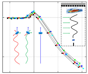
The 3-D trajectories of a bubble in GaInSn recorded by the UPA system are shown in figure 10. The results show that, in the absence of a MF, the path of the bubble follows a zigzag motion, but it does not oscillate strictly in plane, which is consistent with what is predicted in the studies of Tripathi, Sahu & Govindarajan (Reference Tripathi, Sahu and Govindarajan2015) and Sharaf et al. (Reference Sharaf, Premlata, Tripathi, Karri and Sahu2017). This feature differs from the helical path found in numerical studies. However, it should be mentioned that oxide impurities in the GaInSn play an important role in vortex shedding. The contaminated bubbles shed hairpin vortices unsteadily, leading to a zigzag path rather than a helical path (Magnaudet & Eames Reference Magnaudet and Eames2000). As the intensity of the horizontal MF parallel to the Y-direction gradually increases, the bubble transitions to a more strictly zigzag motion, and the oscillations are close to being confined in a plane; eventually, the path instability is gradually suppressed as the trajectory becomes a straight line, similar to the results of Zhang et al. (Reference Zhang, Ni and Moreau2016). Furthermore, we find for the first time that the oscillation plane is first in the direction perpendicular to the MF and then in the direction parallel to the MF. Due to the anisotropy of the bubble oscillation plane, we stipulate that, without a MF, the motion mode is a 3-D random mode (R mode) with a random oscillation plane; when a MF is applied, the motion mode with the oscillation plane perpendicular to the MF is called the vertical mode (V mode) and the mode with the oscillation plane parallel to the MF is called the parallel mode (P mode). During the transition process (T mode), the oscillation plane is gradually turning to the P mode from the V mode. When the bubble finally rises in a vertical path under a strong MF, the motion mode is called a straight mode (S mode). The five motion modes of the bubble are shown in figure 10 for  $Eo=2.43$ as an example.

Figure 10. Variations of motion modes for  $Eo=2.43$ under horizontal MFs. (a) Three-dimensional trajectories. (b) Horizontal motion trajectories, where the directionality of the different motion modes can be seen clearly.
Stable straight rise paths are found when  $B>0.4$ T. Therefore, this study focuses on the oscillation features with $B<0.3$ T. Figure 11 shows the paths of five typical bubbles with different $Eo$ values. To clearly distinguish the directionality of the oscillation plane, the paths in figure 11 are decomposed into two directions. When the oscillations in the X-direction are much stronger than those in the Y-direction, the bubble oscillates in the V mode, and vice versa. Figure 12 presents a flow regime map in the $N-Eo$ space. In order to intuitively express the plane of bubble oscillation, the XOZ plane and YOZ plane are designated as the V-plane and P-plane in this study, respectively.

Figure 11. Three-dimensional trajectories of bubbles with five  $Eo$ values in horizontal MFs with intensities of 0–0.4 T. The black, red, green, blue and cyan lines correspond to $B=0$, 0.1, 0.2, 0.3, 0.4 T respectively. To analyse the anisotropy of bubble oscillations, the trajectories are decomposed into the $X$–
$X$– $Z$ and $Y$–
$Y$– $Z$ planes. Panels show: (a) $Eo=1.13-X$; (b) $Eo=1.13-Y$; (c) $Eo=1.53-X$; (d) $Eo=1.53-Y$; (e) $Eo=1.97-X$; (f) $Eo=1.97-Y$; (g) $Eo=2.43-X$; (h) $Eo=2.43-Y$; (i) $Eo=2.88-X$; (j) $Eo=2.88-Y$.

Figure 12. The  $N-Eo$ map of the bubble motion mode. Bubbles stay in the S mode when $N>1$. The red crosses represent the critical $N$ where the bubble begins to accelerate.
According to our experimental results, it can be seen that the V mode only exists in a narrow range of MF intensity, so there is no relevant report on the V mode of a single bubble in previous experiments and numerical simulations; the P mode has been reported in the numerical simulation of Zhang et al. (Reference Zhang, Ni and Moreau2016) in which a bubble oscillates towards the MF direction at  $N=0.93$. The variation of motion modes may be caused by the 2-D effect of the MF. Based on the classical MHD research (Sommeria & Moreau Reference Sommeria and Moreau1982; Moreau Reference Moreau1990), the MF will suppress the vortices perpendicular to the MF and retain the vortices parallel to the MF, causing the flow to be two-dimensional. Without the MF, the vortex shedding will happen at a random position around the bubble. As the MF gets stronger, the 2-D structures due to the MHD effect appear and the vortices parallel to the MF will be strengthened due to the kinetic energy conversion (Fauve et al. Reference Fauve, Laroche, Libchaber and Perrin1984; Zhang et al. Reference Zhang, Eckert and Gerbeth2007). Therefore, accompanied by the strengthened vortices parallel to the MF, the shedding of the vortex parallel to the MF plays a major role, so the bubble will oscillate perpendicularly to the MF direction, i.e. the V mode, as shown in figure 13.

Figure 13. The diagram of the strengthened flow in the V-plane and non-steady large-scale vortices shedding due to the 2-D effect.
When the MF gets stronger, the bubble will oscillate in P mode. It is known that the MF will suppress  $\boldsymbol {\omega }_x$ and keep $\boldsymbol {\omega }_y$ generated by the bubble. Then $\boldsymbol {\omega }_y$ will be tilted and stretched to cause the accumulation of the streamwise vortex $\boldsymbol {\omega }_z$ according to Legendre & Magnaudet (Reference Legendre and Magnaudet1998). Therefore, the accumulation of $\boldsymbol {\omega }_z$ in the P-plane can be predicted as $N$ gets larger. According to their previous numerical study, Zhang et al. (Reference Zhang, Ni and Moreau2016) found the non-isotropic suppression of the bubble wake by the MF, as shown in the figure 14. Thus, based on the study of Shew & Pinton (Reference Shew and Pinton2006), it can be speculated that the lift force grows in the P-plane due to the distribution of streamwise vorticity, and it causes the bubble to oscillate in this plane. Another possible explanation is conjectured that the P mode may be caused by the overall 2-D circulation in the container. The 2-D effect will become stronger as $N$ increases, leading the 2-D convection rolls to extend along the direction of the MF and form an overall 2-D circulation in the fluid container. Therefore, it will limit the bubble path in the plane parallel to the MF. The physical mechanism of the P mode will be verified in further experimental and numerical studies.

Figure 14. The schematic diagram of the non-isotropic streamwise vorticity distribution after a P-mode bubble based on the study of Zhang et al. (Reference Zhang, Ni and Moreau2016). The dark blue line represents the positive streamwise vorticities and the green line represents the negative, as the vorticities on the backside of the bubble are marked in short dash lines.
According to the  ${\rm \pi}$ theorem from § 3.1, the flow caused by the bubble depends on $Re$,
$Re$,  $Eo$ and $N$, leading to transitions between different modes controlled by these parameters. To study the critical states of the mode transitions, the $N-{Re}^m{Eo}^n$ diagram for the three parameter combinations is plotted. When $m= -1$ and $n = 1.5$, the fits are shown in figure 15. Line 1 represents the fitted line for the transition from the R mode to the V mode, and line 2 represents the fitted line for the transition to the T mode, with their respective fitting formulas as
 \begin{equation}
1000{Re}^{{-}1}{Eo}^{1.5} = \left\{\begin{array}{@{}ll}
-17N+1.8, & Line 1 \\ -5.2N+2.2, & Line 2.
\end{array}\right.
\end{equation}
\begin{equation}
1000{Re}^{{-}1}{Eo}^{1.5} = \left\{\begin{array}{@{}ll}
-17N+1.8, & Line 1 \\ -5.2N+2.2, & Line 2.
\end{array}\right.
\end{equation}
Figure 15. The  $N\sim {Re}^{-1}{Eo}^{1.5}$ map of the bubble motion modes. The black line is the fitted line for the transition from the R mode to the V mode, and the orange line is the fitted line for the transition to the T mode.
It can be seen from figure 15 that all of the bubbles involved in the study experienced four motion modes: from the initial R mode to the V mode, then to the P mode and finally to the S mode. All the bubbles transition to the S mode after  $N=0.95$, which is very close to the equilibrium state of the Lorentz force and the inertial force represented by $N=1$. In the study, it is found that the transition of the larger bubbles occurs earlier as they are more sensitive to the MF, and their motion modes change at smaller MFs.
The relationship between the average relative amplitude  ${A}/{A_0}$ of the bubble oscillations and the interaction parameter $N$ is shown in figure 16, where $A$ is the average amplitude and $A_0$ is the average amplitude with no MF. It is clear that the amplitudes of the three large bubbles decline rapidly when $N\ge 0.5$, while those of the other two smaller bubbles continue to stably decrease until $N\ge 0.75$. This trend also indicates that large bubbles are more sensitive to the MF, also corresponding to the mode transition in figure 15.

Figure 16. Relationship between the average relative amplitude of bubble oscillations and  $N$. The red cross represents the critical $N$ where the bubble begins to accelerate.
3.3. Bubble velocity
The bubble terminal velocity is an important feature of bubble motion. As suggested by Mendelson (Reference Mendelson1967), large bubbles can be treated as interfacial disturbances in an ideal fluid. Consequently, their rise velocities resemble the velocity of a wave propagated over deep water as
 \begin{equation} V_t=\sqrt{\frac{2\sigma}{d_e\rho}+\frac{d_e{g}}{2}} .\end{equation}
In comparison with water, bubbles in GaInSn exhibit higher  $Re$ values due to the significantly greater density difference. This suggests that the influence of viscosity is relatively smaller in GaInSn compared with water. In the absence of a MF, the bubble terminal rise velocities predicted by the Mendelson equation have been verified by the studies of Zhang et al. (Reference Zhang, Eckert and Gerbeth2005), Zhang & Ni (Reference Zhang and Ni2014) and Wang et al. (Reference Wang, Wang, Meng and Ni2017). Thus, the Mendelson equation is employed as the base of velocity of our prediction model under the action of a MF. The results from the Mendelson equation (3.2) are shown in figure 17.

Figure 17. Comparison of terminal velocities of different bubbles obtained by UPA, Mendelson equation, UDV (Zhang et al. Reference Zhang, Eckert and Gerbeth2005; Wang et al. Reference Wang, Wang, Meng and Ni2017) and numerical results (Zhang & Ni Reference Zhang and Ni2014).
It is evident that the velocity,  $V_t$, obtained through the UPA system, agrees favourably with previous experimental findings, which diverge somewhat from the predictions of the Mendelson equation. This discrepancy might be attributed to three factors. First, Mendelson (Reference Mendelson1967) neglected the fluid viscosity in their analysis, assuming that large bubbles functioned as interfacial disturbances akin to waves within an ideal fluid. Consequently, the predicted velocities tend to be higher than the experimental or numerical results. Second, this discrepancy can also be attributed to the oxide impurities, as the size limitations of the MF device makes it challenging to establish an argon-protected environment for GaInSn to avoid oxide impurities. The influence of oxide impurities on the bubble motion characteristics has been emphasized in previous studies. Magnaudet & Eames (Reference Magnaudet and Eames2000) indicated that, when the bubble surface was intentionally contaminated, its trajectory shifted from a helical pattern to a zigzag pattern, a phenomenon consistent with the work of Garner & Hammerton (Reference Garner and Hammerton1954). This explanation elucidates the frequent observation of zigzag paths when the MF is not applied. As Handschuh-Wang, Stadler & Zhou (Reference Handschuh-Wang, Stadler and Zhou2021) revealed, the surface tension of Ga-oxide impurities is smaller than that of the alloy. Therefore, the surface tension is remeasured after the experiment, and the value is found to be 0.515 N m $^{-1}$, which is slightly smaller than the standard value. When considering Ga-oxide impurities in the Mendelson equation with the remeasured surface tension, the difference compared with the standard surface tension is not significant, as shown in figure 17, which indicates that the decrease in the surface tension caused by the impurities is not the main cause of the velocity difference. Additionally, Veldhuis, Biesheuvel & Van Wijngaarden (Reference Veldhuis, Biesheuvel and Van Wijngaarden2008) highlighted that the surface tension gradient attributed to impurities could lead to a no-slip condition on the stagnant bubble cap, thereby augmenting the drag experienced by the bubble. Consequently, the velocities computed through direct simulations by Zhang & Ni (Reference Zhang and Ni2014) are lower than those obtained through the Mendelson equation predictions due to the latter's disregard of the viscosity. Furthermore, the experimental results diverge further from Mendelson's predictions due to the no-slip condition on the stagnant bubble cap. Considering that the $V_t$ values obtained by the UPA are basically consistent with those obtained by the UDV, the bubble terminal velocities measured in the study are considered to be acceptable.
The horizontal MF will greatly influence the bubble velocity characteristics. As an example, the bubble velocities with  $Eo=2.88$ for various MF intensities are shown in figure 18. It can be seen that, in the absence of the MF, the bubble velocity increases rapidly to a maximum velocity of approximately 250 mm s $^{-1}$, and then it drops to approximately 220 mm s $^{-1}$ with oscillations. The varying velocity trend agrees with that reported by Shew & Pinton (Reference Shew and Pinton2006), who conducted a study on the zigzag bubble velocity. When the MF intensity increases, the velocity stays in an oscillating state for $N<1$. However, these oscillations are significantly weakened as $N$ increases and disappears when $N\ge 1$. The weakened velocity oscillations are consistent with the changes in the bubble trajectories and the reductions in relative amplitudes are described in the previous section.

Figure 18. Oscillating velocity of the bubble ( $Eo=2.88$) as $N<1$.
The relationship between the dimensionless terminal velocity  ${V_t}^{\ast }={V_t}/{V_{t0}}$ and $N$ is shown in figure 19, where $V_{t0}$ is the terminal velocity without a MF. It can be concluded that the ${V_t}^{\ast }$ values of all the bubbles with various $Eo$ values in the experiments increase with the increase in $N$, and the maximum value occurs near $N=1$, which has also been found in the previous experimental research (Wang et al. Reference Wang, Wang, Meng and Ni2017). The inertial and Lorentz forces will reach a balance when $N=1$, and while the MF becomes stronger ( $N>1$), the velocity will decline rapidly with increasing $N$.
$N$.

Figure 19. Dimensionless velocities of five bubbles under a large range of  $N$.
$N$.
According to the experimental results, the velocity increase is closely related to the motion mode and relative amplitude. The  $N$ thresholds at which the bubbles begin to accelerate are directly dependent on the bubble size. For example, ${V_t}^{\ast }$ with $Eo=1.13$ begins to grow at $N=0.6$, while for $Eo=2.88$, $N=0.32$. The $N$ threshold at which ${V_t}^{\ast }$ begins to increase significantly is denoted as $N_T(Eo)$. With the $N_T(Eo)$ plots of the five bubbles shown in figure 16, it can be concluded that, in the initial R mode, the subsequent V mode and the T mode, the oscillation amplitudes of the bubbles decrease slightly, and the corresponding bubble velocities show no significant changes. The bubbles begin to accelerate when $N$ is slightly larger than the $N$ threshold of the P mode. Moreover, it can be determined that, near $N_T(Eo)$, the relative amplitude ${A}/{A_0}$ experiences more significant damping. This relationship between the bubble velocity and path was also suggested by Zhang et al. (Reference Zhang, Eckert and Gerbeth2005), who showed that the reduction of the drag coefficient may result from a modification of the bubble path caused by the MF.
When  $N>1$, all the bubbles enter the S mode. The velocities decrease rapidly with the enhancement of the MF under the action of the Lorentz forces. Because the velocity oscillations are suppressed, the bubble drag force $F_d=({{\rm \pi} }/{2})\rho _l({d_e}/{2})^2{C_d}{V_t}^2$ is balanced with the buoyancy force $F_b=({4{\rm \pi} }/{3})\Delta \rho {g}({d_e}/{2})^3$ when an equilibrium state is reached. Therefore, the drag coefficient $C_d$ can be calculated by
 \begin{equation} C_d=\frac{4\Delta\rho{d_e}g}{3{V_t}^2{\rho_l}} .\end{equation}
 The parameter  $C_d$ satisfies the scaling rule $C_d \propto N^{0.5}$, as shown in figure 20. This scaling rule also agrees with those of Yonas (Reference Yonas1967) and Pan, Zhang & Ni (Reference Pan, Zhang and Ni2018) for a particle in a liquid metal under a MF with different $Re$ values. This means that, under a strong MF, the drag coefficient and $N$ will always obey the same scaling law, regardless of $Re$ and the geometric shape.

Figure 20. Drag coefficient  $C_d$ satisfies the relationship of $C_d \propto N^{0.5}$.
Considering the experimental results without a MF shown in figure 17, the bubble terminal velocity in GaInSn predicted by the Mendelson equation (3.2) can be modified as
 \begin{equation} V_{tr}=0.85\sqrt{\frac{2\sigma}{d_e\rho_l}+\frac{d_eg}{2}} .\end{equation}
In the modified equation, a correction factor of 0.85 is applied to comprehensively consider the influence of the viscosity and oxide impurities. The modified velocity prediction curve is closer to the experimental results, as shown in figure 21.

Figure 21. Equation (3.4), the modified bubble terminal velocity prediction equation in GaInSn. In this figure the equation is compared with experimental results.
Based on the experimental results, the dimensionless terminal velocity of the bubbles in GaInSn under the influence of a MF, denoted as  ${V_t}^\ast (N)=V_t/V_{tr}$, can be categorized into three distinct stages: the invariable velocity stage for $0< N< N_T(Eo)$, the increasing stage for $N_T(Eo)\le {N}<1$ and the descending stage for $N\geq 1$. The critical $N$ at which the bubble begins to accelerate, denoted as $N_T(Eo)$, is determined by averaging the results obtained with individual $Eo$ values. As a result, we obtained five $N_T(Eo)$ values corresponding to five different bubbles. Subsequently, a fitted function can be formulated to describe the dependence of $N_T(Eo)$ on $Eo$
$Eo$
 \begin{equation} N_T(Eo)=0.52{Eo}^{{-}1.5}. \end{equation}
The graphical representation of this fitted function can be found in figure 22.

Figure 22. Comparison of (3.5) and  $N_t(Eo)$ obtained in this paper.
During the invariable velocity stage, the velocities remain essentially consistent with those observed without the presence of the MF. In the increasing stage, due to the relatively minor velocity variations from  ${V_t}^\ast$, precise formulation of a velocity prediction equation becomes challenging. Hence, further investigations are required to accurately determine this relationship. Nonetheless, a consistent deceleration trend ${V_t}^\ast (N)\sim {N}^{-0.25}$ is evident when $N\geq 1$. Considering the influence of $Eo$, the velocity prediction equation for $N\geq 1$ is derived as
 \begin{equation} {V_t}^\ast(N)=1.038{Eo}^{0.1}N^{{-}0.25},\quad N\geq1 .\end{equation}
This prediction equation is depicted graphically in figure 23.

Figure 23. The comparison of the dimensionless predicted velocity  ${V_t}^\ast (N)$ and the experimental results when $N\geq 1$.
4. Conclusions
The motion characteristics of bubbles in a liquid metal under the action of a horizontal MF, including the oscillation trajectories and the rise velocities, are experimentally studied. To study the bubble motion in opaque liquids, a UPA system is introduced and its ability to detect bubbles as moving defects in a liquid metal is verified.
With a gradually increasing MF, the bubbles in the GaInSn experience four different motion modes: from the initial R mode to the V mode and then to the P mode (with a T mode between the V and P modes) and finally to the S mode. The transition of the motion modes occurs with a small  $N$ and a large $Eo$, indicating that a larger bubble is more sensitive to the MF. With $N\approx 1$, a bubble almost loses its path instabilities and rises straight. The anisotropy of the oscillation direction at a moderate $N$ is revealed for the first time. The variation of the terminal velocity is closely related to the transition of the motion mode. Magnetic fields with $N<1$ suppress the path oscillations but also increase the terminal velocity $V_t$, which reaches its maximum value around $N=1$. This increasing tendency of $V_t$ is consistent with the suppression of the oscillation amplitude, which indicates that the energy originally lost in the horizontal oscillations is partially converted into $V_t$. For $N>1$, all of the bubbles enter the S mode in which MFs monotonically suppress $V_t$ satisfying the scaling law ${V_t}\propto {N}^{-0.25}$, and the computed drag coefficient $C_d$ satisfies the scaling law of $C_d\propto {N}^{0.5}$.
Funding
The authors gratefully acknowledge the supports from National Key Research and Development Program of China (#2022YFE03130000), and from NSFC (#11872362, #51927812, #52176089).
Declaration of interests
The authors report no conflict of interest.


