


1. Introduction
Gravity currents (GCs) develop whenever there is a density difference between the current fluid, with density  $\rho _c$, and the ambient fluid, with density $\rho _a$. These currents propagate at the bottom of the ambient fluid when $\rho _c > \rho _a$ (hyperpycnal), or at the top of the ambient fluid in the opposite case (hypopycnal). If the ambient fluid is stratified, currents propagate at the level of equal density (mesopycnal). The current and ambient fluid are not necessarily different, as a difference in density may be related to a difference in temperature or to suspended particles inside the heavier fluid. Many examples of GCs occur in natural environments, such as dust and sand from a turbulent wind, avalanches of small snowflakes that grow flowing along the hazardous slopes of mountains or cold air near the floor of a room coming in from an opened window. More examples can be found in the extensive monographs by Simpson (Reference Simpson1999) and Huppert (Reference Huppert2006).
GCs are often classified on the basis of the terms that dominate the momentum balance, distinguishing inertial–buoyancy and viscous–buoyancy regimes. In the presence of obstacles or vegetation, the balance can also be turbulent drag–buoyancy. There are several possible sources of turbulent drag; it can be associated with entrainment with the ambient fluid and with the structure of the flow field (see, e.g., Lane-Serff Reference Lane-Serff1993), or with the presence of obstacles that are spatially extended. The presence of turbulent drag suggests an analogy between GC flow and flow in the Forchheimer regime in porous media (Hatcher, Hogg & Woods Reference Hatcher, Hogg and Woods2000), with a velocity profile that appears uniform in the vertical and with dissipation controlled by the obstacles, with negligible bottom effects. If the GC can spread over a sufficient space, a transition is expected with the current initially in the inertial–buoyancy regime, then in the viscous–buoyancy regime depending on the Reynolds number (with the exception of critical GCs, see Maxworthy Reference Maxworthy1983; Chiapponi et al. Reference Chiapponi, Ungarish, Longo, Di Federico and Addona2018). In the presence of turbulent drag, a further transition is expected, with inertia initially dominant, then overtaken by turbulent drag and finally replaced by viscous drag.
The behaviour of the stream is conditioned by the release mechanism at the source: a lock release (LR) consists of a finite volume of current released instantaneously into the environment, whereas a constant-flow or a time-varying flow current is a flow continuously fed from a source at a constant or time-varying flow rate; in the latter case waxing or waning flows rate can be modelled. Many simplifications can be adopted in the models, whether the ratio  $\rho _a/\rho _c \approx 1$ or not (Boussinesq and non-Boussinesq currents), or the dynamics of the ambient fluid can be neglected in the propagation characteristics of the current (single layer model). For more details, see the recent comprehensive book by Ungarish (Reference Ungarish2020).
The great interest in this broad natural phenomenon, and the enormous variety of configurations in the environment and industry, has stimulated a rich line of theoretical and experimental research, with advanced numerical techniques and sophisticated measuring instruments. The simplest configuration, with a horizontal bottom, is perhaps the one most intensively investigated, starting with Benjamin's pioneering publication (Benjamin Reference Benjamin1968) with numerous extensions to a general cross-section (Ungarish Reference Ungarish2018), and with stratification of the ambient fluid (Longo et al. Reference Longo, Ungarish, Di Federico, Chiapponi and Addona2016).
More complex models refer to particle-driven currents (Sparks et al. Reference Sparks, Bonnecaze, Huppert, Lister, Hallworth, Mader and Phillips1993; Hogg, Ungarish & Huppert Reference Hogg, Ungarish and Huppert2000; Zemach et al. Reference Zemach, Chiapponi, Petrolo, Ungarish, Longo and Di Federico2017; Lippert & Woods Reference Lippert and Woods2020). Sher & Woods (Reference Sher and Woods2017) described the relative importance of entrainment at the interface and particle sedimentation in controlling the run-out distance of short-lived GCs, and the influence of an up-slope boundary has been considered by Ottolenghi et al. (Reference Ottolenghi, Adduce, Inghilesi, Roman and Armenio2016), Martin et al. (Reference Martin, Negretti, Ungarish and Zemach2020) and De Falco et al. (Reference De Falco, Adduce, Negretti and Hopfinger2021). Recent studies (Longo et al. Reference Longo, Ungarish, Di Federico, Chiapponi and Petrolo2018; Sciortino, Adduce & Lombardi Reference Sciortino, Adduce and Lombardi2018; Chiapponi et al. Reference Chiapponi, Ungarish, Petrolo, Di Federico and Longo2019) have focused on the effects of a free top, such as a superficial depression bounded to the advancing nose; these effects are usually neglected.
In the vast majority of cases, models refer to currents advancing in a confined section with hydraulically smooth walls, or on a smooth bottom. However, almost always ambient GCs interact with obstacles of various kinds, as happens for flows through forests, urban and aquatic canopies, as documented in many reviews (Finnigan Reference Finnigan2000; Belcher, Harman & Finnigan Reference Belcher, Harman and Finnigan2012; Nepf Reference Nepf2012). Vegetation-like obstacles are often modelled as flexible or rigid vertical cylinders with diameter  $D$ and height $h$, with $h$ being smaller or larger than the ambient-fluid height $H$, and vegetation is said to be submerged when $h< H$. A relevant parameter is the density of the vegetation, $\kappa = n A_c/A$, defined as the ratio of the plane area occupied by the cylinders, $n A_c$, to the total area of the lower base of the channel, $A$, where $n$ is the total number of cylinders and $A_c = {\rm \pi}D^2/4$ is the cross-sectional area of a single cylinder.
LR GCs in the presence of artificial vegetation (thin flexible plastic tubes) have been studied, e.g. by Naftchali et al. (Reference Naftchali, Khozeymehnezhad, Akbarpour and Varjavand2016), who carried out experiments with  $\kappa$ in the range $[0.006, 0.014]$ and found that, for increasing $\kappa$, the current velocity decreases up to $28.5\,\%$, while the density of the current $\rho _c$ decreases up to $82\,\%$ as a consequence of mixing. When $\kappa$ is small, any small change in $\rho _c$ does not cause a significant change in the forward velocity of the current. Cenedese, Nokes & Hyatt (Reference Cenedese, Nokes and Hyatt2018) (experiments with vertical rigid cylinders) found that, when the current height is smaller than the vegetation height, the current front has a triangular shape, but when the current is higher than the vegetation, two different regimes develop for the small (sparse arrays) and large (dense arrays) $\kappa$ respectively: (i) in the sparse array configuration ( $\kappa =0.09$), the denser fluid current propagates between the cylinders with high entrainment enhanced by the vortices generated in the wake of the cylindrical obstacles; (ii) in the dense array configuration ( $\kappa =0.35$), the denser fluid current is almost entirely above the vegetation, where the drag force is lower, and undergoes convective instability, mixing vertically with the environment and diluting near the nose.
In more complex situations, vegetation and the presence of shallow water promote density stratification of thermal origin and the onset of a GC. Zhang & Nepf (Reference Zhang and Nepf2008) studied the effects of different heat exchanges between the open water and the canopy (they used a random array of rigid, emergent cylinders to represent the canopy region), a configuration with the water within the submerged vegetation absorbing less solar heat than the adjacent deep water. They found that the velocity of the current is reduced by the drag of the canopy in the vegetative region, while in the open region the velocity of the current remains constant and depends only on the initial conditions. Numerical simulations indicate that, in both partially and fully vegetated regions, currents are inertial for  $C_D \xi _T l_c < 10$, where $C_D$ is the drag coefficient, $\xi _T = n D/A$ is the array density (fraction of the frontal area of cylinders per unit volume, where $A$ is the bed area and $\xi _T$ has dimension of $L^{-1}$), and $l_c$ is the total length of the current, provided that $C_D \xi _T H/n < 13.39$. When $C_D \xi _T H/n > 13.39$, currents are entrained due to the high vegetation density and short inertia flow time period (Tsakiri, Prinos & Koftis Reference Tsakiri, Prinos and Koftis2016).
Testik & Ungarish (Reference Testik and Ungarish2016) conducted a theoretical analysis on both LR and continuous-flow GCs in a rectangular channel in the presence of artificial vegetation (cylindrical rods), comparing the results with previous experimental studies by Hatcher et al. (Reference Hatcher, Hogg and Woods2000), Tanino, Nepf & Kulis (Reference Tanino, Nepf and Kulis2005) and Testik & Yilmaz (Reference Testik and Yilmaz2015). Testik & Ungarish (Reference Testik and Ungarish2016) solved a more general model, in which the drag force is proportional to  $|u|^ \lambda$, with $u$ being the horizontal velocity and $\lambda$ a constant positive value. They found four classes of similarity solutions: class I describes GCs with a triangular shape and constant velocity at the nose, which is developed with a continuous-release source; class II GCs have a fixed height at the source and a nonlinear profile, but with no experimental evidence yet; class III corresponds to constant-volume GCs with a linearly increasing velocity toward the nose; all other continuous-release GCs belong to class IV.
The present experimental activity refers to GCs in a cylindrical axisymmetric geometry in the presence of artificial vegetation, to achieve more insights into the physical process. This configuration is representative of many environmental scenarios (see Chowdhury & Testik (Reference Chowdhury and Testik2014) for a long list), for example in the presence of localized inputs in the absence of flow channelization, or during disposal operations of dredged materials for beaches and wetland restoration (pipelines for conveying mixtures of water and sediment have a terminal that represents a localized source, coinciding with the origin of a radially symmetrical discharge, and trigger turbidity currents; pile and sheet pile driving in a lake or marine environments generates radially symmetrical turbidity currents, which pose an environmental risk and disturbance to aquatic species). These GCs in a radial geometry appear of particular interest, compared with the case of GCs confined in a rectangular (non-divergent) geometry.
We conducted 40 experiments with two different densities of the array of the artificial vegetation: 12 in the LR configuration, 13 in constant inflow rate, 9 in waxing and 6 in waning inflow rate. To the best of our knowledge, the experiments are original and new, and no similar experiments are available in the literature.
Although the vegetation of our experiments is artificial, with pragmatic choices of the dimensions of the rods dictated by experimental needs and by commercial availability of the items requested for the set-up, the adopted pattern reflects realistic aquatic vegetation. In fact, defining the frontal area per unit volume  $a=D/s^2$, where $s$ is the spacing between rods, our experimental configuration corresponds to $a=0.066\text {--}0.138\ \textrm {cm}^{-1}$, which is equivalent to marsh grasses with $a=0.01\text {--}0.07\ \textrm {cm}^{-1}$, Seagrasses with $a=0.01\text {--}0.07\ \textrm {cm}^{-1}$ and mangroves with $a$ up to $0.2\ \textrm {cm}^{-1}$ (Nepf Reference Nepf2012).
The available theoretical models point out that GC propagation analysis is inconclusive when the value of  $\lambda$ is not known (Testik & Ungarish Reference Testik and Ungarish2016), hence we measured the drag exponent, with the same pattern of rods adopted for GC experiments (same density) and for different values of the Reynolds number. We also expect the $\lambda$ exponent of drag to be a function not only of Reynolds number and density of the obstacles, but also of other geometric characteristics of the obstacles, such as, for example, the frontal area per unit volume (see, e.g., Ozan, Constantinescu & Hogg Reference Ozan, Constantinescu and Hogg2015) or the diameter of the rods or of an equivalent size for other obstacles. If the flow of the GCs were in a classical porous medium, we would expect a dependence on ‘permeability’; in the present case we expect a dependence on the spacing between obstacles or on the diameter of the rods, and two further drag measurements were performed with a different diameter of the rods in order to elucidate this aspect. However, we bear in mind that the goal of the present analysis is not the identification of such a dependence, but more pragmatically the estimation of the exponent $\lambda$ to be used for the interpretation of the experiments. The physical limits are $\lambda =1$ for viscous drag at low Reynolds number, and $\lambda =2$ in the fully turbulent regime at high Reynolds number.
The paper is organized as follows. Section 2 briefly introduces the theoretical model, § 3 describes the experimental layout and procedures and § 4 provides details and discussion on the experiments. The conclusions are drawn in § 5. The results of drag measurements with different rods diameters are analysed in Appendix A, where scaling of drag is discussed with respect to the density and the diameter of the rods.
2. Theoretical model for vegetation domain
2.1. Formulation
Here, we present the essentials of the theoretical model used in our investigation. This model served a guideline for the design and set-up of the experiments, and it is also used for comparisons with, and interpretation of, the data and effects recorded in our experiments. We note that the model has been presented before (Hatcher et al. Reference Hatcher, Hogg and Woods2000; Testik & Ungarish Reference Testik and Ungarish2016). The novelty here is the application of new influx conditions and the comparison with experiments aiming to an estimate of the power-law  $\lambda$ and to measure the front position and the profile of the currents.
We use a cylindrical coordinate system, and assume axial symmetry (i.e. zero or negligibly small dependency on the angular coordinate). We consider rod-like vegetation which fills a horizontal domain of height  $H$. In our system of reference, the coordinate $r$ is horizontal, while $z$ is vertically upward. The GC propagates in the $r$ direction, see figure 1(a). The densities of the current and ambient fluids are $\rho _{c}$ and $\rho _{a}$, with $\rho _{a} <\rho _{c}$, and $z=0$ and $z=H$ are rigid boundaries, see figure 1(b). For practical reasons, $z=H$ in the experiments is a free surface, see next discussions on the sensitivity of the results to this approximation. The height (thickness) of the current is $h(r,t)$, and the height-averaged speed of the current is $u(r,t)$, while that of the ambient is $u_a(r,t)$. The radius of propagation is $r_N(t)$.
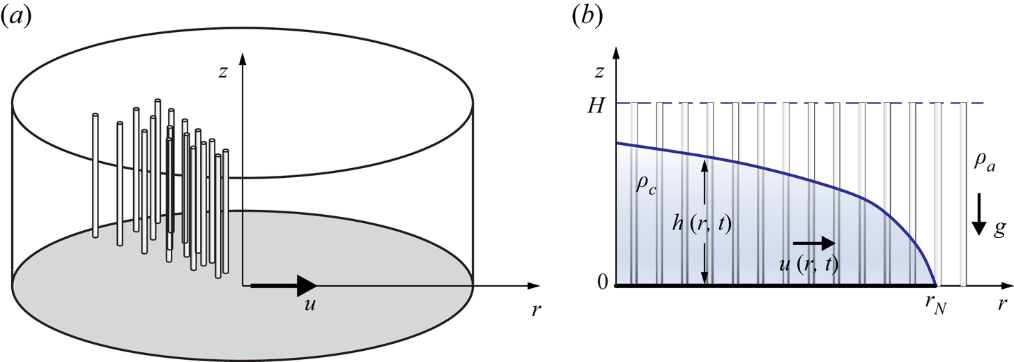
Figure 1. Sketch of the theoretical model: (a) three-dimensional schematic; (b) axial-radial plane section.
The equations of motion are derived along the lines of the thin-layer simplification detailed in Ungarish (Reference Ungarish2020). We use dimensional variables unless stated otherwise.
2.2. Equations of motion and boundary conditions
We start with the observation that the thickness of the ambient-fluid layer is  $H-h$ and by continuity
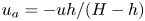 \begin{equation} u_a ={-} u h /(H - h) \end{equation}
for constant  $H$. The vegetation introduces a drag force. As suggested by previous investigations and confirmed by our experiments, the effective drag per unit volume of fluid is proportional to the density of the fluid and to the speed at some power $\lambda \ge 1$. To facilitate the analysis, we assume that (i) the coefficient of proportionality is a constant, $\tilde {c}$; (ii) in a given GC system, both the current and the ambient have the same $\tilde {c}$ and $\lambda$ (as will be evident in the following steps, the accuracy of this assumption is not relevant since we will adopt a single-layer model where only the dynamics of the dense current is considered). We assume (and confirmed by order of magnitude estimates of the laboratory data) that, in the tests considered here, the viscous and turbulent stresses in the current and ambient domains are negligible as compared with the other forces. We consider flow fields in which the drag dominates the acceleration (inertia) term. Therefore, in the subsequent analysis the $\textrm {D}u/\textrm {D}t$ terms are neglected, except for the analysis of transition, see (2.7). The pressure is approximated by the hydrostatic balance, and hence the
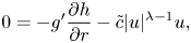
  $x$-momentum balances for the ambient and current reduce to
 \begin{equation} 0={-}\dfrac{\partial p}{\partial x}-\rho_a\tilde{c}u_a|u_a|^{\lambda-1},\quad 0={-}\dfrac{\partial p}{\partial x}-(\rho_c-\rho_a)g\dfrac{\partial h}{\partial r}-\rho_c\tilde{c}u|u|^{\lambda-1}, \end{equation}
where  $p$ is the reduced pressure in the ambient and $g$ the gravity acceleration. Here, $\lambda$ is assumed to be constant. Elimination of the pressure and use of (2.1) yield one combined-momentum equation for $u$. Consequently, the motion can be expressed as the system of continuity and momentum balances
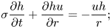 $$\begin{gather} \sigma \frac{\partial h}{\partial t} + \frac{\partial h u }{\partial r} ={-}\dfrac{u h}{r}; \end{gather}$$
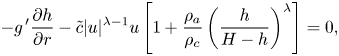 $$\begin{gather}- g^{\,\prime} \frac{\partial h}{\partial r} - \tilde{c} |u|^{\lambda-1}u \left [ 1 + \frac{\rho_{a}}{\rho_{c}} \left( \dfrac{h}{H-h} \right)^\lambda \right ]=0, \end{gather}$$
where the reduced gravity is  $g^{\prime } = g(1- \rho _{a}/\rho _{c})$, and $\sigma$ is the porosity of the vegetation medium in which the fluids move, always positive and smaller than $1$, assumed here constant. We also define the density of the vegetation as $\kappa = 1-\sigma$.
Further simplifications of the equations are possible and useful. First, we introduce the coordinate stretching of the time to  $t/\sigma$; this eliminates $\sigma$ from the subsequent analysis. Second, we note that the Boussinesq system with $\rho _{c} \approx \rho _{a}$ admits the simplification of the drag term in the momentum equation (2.4) by setting $\rho _{a}/\rho _{c} = 1$ in front of the term $h/(H-h)$ which expresses the drag coupling between the current and the upper ambient fluid. Next, for a deep current $h/H \ll 1$, the coupling term can be neglected. This simplification, also called the one-layer model, is facilitated by the fact that the value of $\lambda$ is larger than 1 and typically $2$. In the range of parameters considered in the present investigation, the model based on Boussinesq and one-layer simplifications is expected to provide a fair approximation to the main behaviour (propagation and shape) of the current. The one-layer theory is an approximation that is expected to work well when the height of the current to ambient at $r/r_N \approx 0.5$ is less than 0.5 (which implies that a significant part of the current is even thinner), and when the rate of increase of the height due to influx is much smaller than the speed of propagation. (We keep in mind that $h$ decreases with $r$ and that the propagation of the current is governed by the ring of fluid close to $r_N$). Consequently, we shall use the momentum equation
 \begin{equation} 0 ={-} g^{\prime} \frac{\partial h}{\partial r} - \tilde{c} |u|^{\lambda-1}u, \end{equation}
which expresses the balance between the buoyancy driving force and the vegetation-drag hindering effects on the layer of the dense fluid. We note that the curvature terms are not present in this balance; however, the curvature effect is strongly manifested on the right-hand side continuity (2.3) and hence the present geometry needs a separate investigation from the two-dimensional Cartesian counterpart.
We emphasize that the coefficient  $\tilde {c}$ in the drag term is different from the classical dimensionless ‘drag coefficient’ defined by the ratio of non-viscous opposing force on a body to dynamic pressure. The present drag coefficient is defined by the ratio of the opposing force between vegetation and fluid, per unit volume of fluid, divided by $\rho |u|^\lambda$ (the density and speed pertain to either the domain of the current or ambient), and $\tilde {c}$ is dimensional with $[\tilde {c}]=L^{1-\lambda }T^{\lambda -2}$.
In general, the volume of the current is known. This can be expressed as
 \begin{equation} \int_0^{r_N(t)} r\,h(r,t)\, \textrm{d}r =qt^{\alpha}\equiv \mathcal{V}(t), \end{equation}
where  $q$ and $\alpha \ge 0$ are given constants. Note that $\mathcal {V}(t)$ is the volume per radian, and contains both fluid and vegetation.
At the nose  $r= r_N(t)$, we impose the condition $h=0$ while $u_N$ is finite. The justification is as follows. The motion takes place because the buoyancy driving $g^{\prime } (- \partial h/\partial r)$ in the radial direction balances the opposing drag $\sim - |u|^{\lambda -1}u$. This means that, at any radial position of the moving current, a negative slope $\partial h/\partial r$ is present, and hence $h$ is expected to decrease to $0$ at the nose. The subsidiary assumption is that a nose of zero thickness (i.e. a contact line) is compatible with the equations of motion, and this will be confirmed later. (We note in passing that a moving contact-line condition is an abstraction of a complex $r$-thin corner region in which strong gradients are present, and hence in practice the decrease to $h=0$ is less sharp than in the theory. There is evidence from the viscous-current counterpart, see Ungarish (Reference Ungarish2020), that this singularity has little effect on the speed of propagation, because the larger $h$ creates a larger buoyancy drive from the dense material behind. We conjecture that the same behaviour occurs in the present case.) In this context we also note that it is possible to eliminate $u$ from (2.3) and (2.5) to obtain one equation for $h(r,t)$, which bears similarity with the formulation for power-law fluid GCs, see for example Sayag & Worster (Reference Sayag and Worster2013).
For the boundary conditions at the axis  $r=0$, we must distinguish between the following cases: (i) fixed volume (or LR) admits the simple $u=0$ at $r=0$; (ii) for GCs created by influx, it is in general difficult to prescribe the precise boundary condition at the source. What we usually know is the total volume flux. Near the axis, the influx speed may be large and the thin-layer assumptions may be invalid. From the point of view of the present set of equations, this domain is a singularity. For progress, we apply the usual assumption that there is some adjustment domain in which the flux is matched with the values of $h$ imposed by the outer region. The relative volume of fluid in this singular region is expected to be small with respect to the volume of the dense fluid, (the radial geometry embeds a bottom area growth proportional to the square of the radius and we are considering the region near the axis) and, hence, of little relevance to the major flow field (see Di Federico, Archetti & Longo Reference Di Federico, Archetti and Longo2012). The generally accepted mathematical solution for the axisymmetric current created by influx imposes the conditions at the nose, but leaves open the behaviour near the axis. We shall keep this in mind during the comparisons with realistic data.
In the present simplified model, we cannot apply realistic initial conditions of  $u$ and $h$ at $t=0$. The physical meaning is that the initial inertial adjustment is missed, and we assume that this adjustment is a short episode, whose details are insignificant to the subsequent motion.
2.3. Regimes of GCs
An estimate of the transition from the buoyancy–inertial to buoyancy–drag (turbulent drag) regime can be obtained by imposing that the flow inertia, drag and buoyancy terms are of the same order of magnitude
 \begin{equation} \dfrac{\partial u}{\partial t}\sim g^{\prime}\dfrac{\partial h}{\partial r}\sim\tilde{c}|u|^{\lambda-1}u, \end{equation}
while the mass conservation in integral form brings  $hr^2\sim \mathcal {V}$. By assuming that $r\sim u t_c$ and $\mathcal {V}=qt^\alpha$, and defining $t_c$ as the time of transition, we get
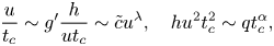 \begin{equation} \dfrac{u}{t_c}\sim g^{\prime}\dfrac{h}{ut_c}\sim \tilde{c}u^{\lambda},\quad hu^2t_c^2\sim qt_c^\alpha, \end{equation}
which leads to the scaling
 \begin{equation} t_c\sim (g^{\prime} q \tilde{c}^{4/(\lambda -1)})^{(1-\lambda)/[\alpha (\lambda -1)-2 \lambda +6]}, \end{equation}
equal to
 \begin{equation} t_c\sim\tilde{c}^{{-}1};\quad (\tilde{c}^{4} g^{\prime} q)^{{-}1/(\alpha +2)}\quad\textrm{for}\ \lambda=1,2. \end{equation}
The critical time increases with  $\lambda$ and decreases with $\alpha$. Later on a viscous–buoyancy balance dominates, at a time obtained by imposing that the viscous drag, turbulent drag and buoyancy terms are of the same order of magnitude
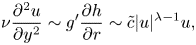 \begin{equation} \nu\dfrac{\partial^2u }{\partial y^2}\sim g^{\prime}\dfrac{\partial h}{\partial r}\sim\tilde{c}|u|^{\lambda-1}u, \end{equation}
or
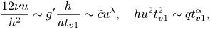 \begin{equation} \dfrac{12\nu u}{h^2}\sim g^{\prime}\dfrac{h}{ut_{v1}}\sim \tilde{c}u^{\lambda},\quad hu^2t_{v1}^2\sim qt_{v1}^\alpha, \end{equation}
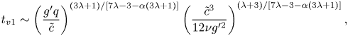
which leads to the scaling
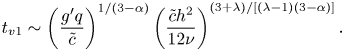 \begin{equation} t_{v1}\sim \left(\dfrac{g^{\prime} q}{\tilde{c}}\right)^{1/(3-\alpha)}\left(\dfrac{\tilde{c}h^2}{12\nu}\right)^{(3+\lambda)/[(\lambda-1)(3-\alpha)]}. \end{equation}
Considering the viscous drag due to the obstacles, instead of the viscous drag due to the bottom, results in
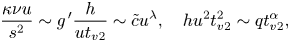 \begin{equation} \dfrac{\kappa\nu u}{s^2}\sim g^{\,\prime}\dfrac{h}{ut_{v2}}\sim \tilde{c}u^{\lambda},\quad hu^2t_{v2}^2\sim qt_{v2}^\alpha, \end{equation}
where  $s$ is a scale of the spacing of the obstacles and $\kappa$ is the density of the obstacles. The corresponding time of transition is
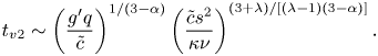 \begin{equation} t_{v2}\sim \left(\dfrac{g^{\prime} q}{\tilde{c}}\right)^{1/(3-\alpha)}\left(\dfrac{\tilde{c} s^2}{\kappa\nu}\right)^{(3+\lambda)/[(\lambda-1)(3-\alpha)]}. \end{equation}
Note that, for  $\lambda =1$, the two times $t_{v1}$ and $t_{v2}$ are undefined since viscous resistance and drag scale with $u$ and are indistinguishable. In conclusion, the obtained self-similar solution is intermediate asymptotic in the interval $t_c< t< t_v$ where $t_v=\min (t_{v1},t_{v2})$. The condition $t_{v2}< t_{v1}$ corresponding to viscous drag due to vegetation dominating with respect to the viscous drag due to the bottom, for $\alpha <3$ requires that $s< h\sqrt {\kappa /12}$, which for $\kappa =0.10$ and $h=1\ \textrm {cm}$ indicates $s\approx 1\ \textrm {mm}$, a condition generally not satisfied. A waxing inflow rate with $\alpha >3$ is unrealistic and, moreover, we expect it to occur for a short time interval, not sufficient to allow viscosity to dominate the balance with buoyancy. For this reason, we limit our analysis to a viscous–buoyancy balance regime due to the floor of the tank and not to the vegetation. The previous results for $\lambda =2$ correspond to values given in Hatcher et al. (Reference Hatcher, Hogg and Woods2000).
Equation (2.13) can be also expressed as a function of the parameters of the flow process as
 \begin{equation} t_{v1}\sim\left(\dfrac{g^{\prime} q}{\tilde{c}}\right)^{(3 \lambda +1)/[7 \lambda -3-\alpha (3 \lambda +1)]}\left(\dfrac{\tilde{c}^3}{12 \nu g^{\prime 2}}\right)^{(\lambda +3)/[7 \lambda -3-\alpha (3 \lambda +1)]}, \end{equation}
where  $h$, retained in (2.13) only for comparing $t_{v1}$ and $t_{v2}$, has been eliminated. Equating (2.9) and (2.16) yields a time scale $t^*$ and volume coefficient scale $q^*$
$q^*$
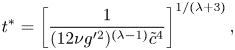 $$\begin{gather} t^*=\left[\dfrac{1}{(12 \nu g'^2)^{({\lambda-1 })}\tilde{c}^{4}}\right]^{1/(\lambda+3)} , \end{gather}$$
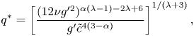 $$\begin{gather}q^*=\left[\dfrac{(12 \nu g'^2)^{\alpha (\lambda -1)-2 \lambda +6} }{ g'\tilde{c}^{4 (3-\alpha)}}\right]^{1/(\lambda+3)}, \end{gather}$$
that allow us to express the two times in dimensionless form
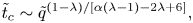 \begin{equation} \tilde{t}_c\sim \tilde{q}^{(1-\lambda)/[\alpha (\lambda -1)-2 \lambda +6]}, \end{equation}
and
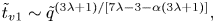 \begin{equation} \tilde{t}_{v1}\sim\tilde{q}^{(3 \lambda +1)/[7 \lambda -3-\alpha (3 \lambda +1)]}, \end{equation}
where  $\tilde {t}=t/t^*$ and $\tilde {q}=q/q^*$. The exponent in (2.19) is always negative for $1<\lambda <2$ and $\alpha >0$, and $\tilde {t}_c$ monotonically decreases with $\tilde {q}$. The exponent in (2.20) is positive if $\alpha <\alpha _c\equiv (7\lambda -3)/(3\lambda +1)$ and it is negative otherwise. Figure 2(a) shows the theoretical dimensionless times vs the volume coefficient, as a function of $\alpha$ and for $\alpha <\alpha _c$. The hatched area refers to $\alpha =0$ and $\lambda =2$ and is the domain of existence of an intermediate asymptotic similarity solution, which is possible only for $\tilde {q}>1$: the initial stage of the GC is dominated by inertia, which progressively becomes less important leaving space to turbulent drag of the vegetation. The turbulent drag–buoyancy balance is finally substituted by a viscous–buoyancy balance. The domain of existence of the turbulent drag–buoyancy balance widens with $\alpha$ and also for reduced $\lambda$, and for $\alpha \to \alpha _c$ viscosity never dominates over turbulent drag.
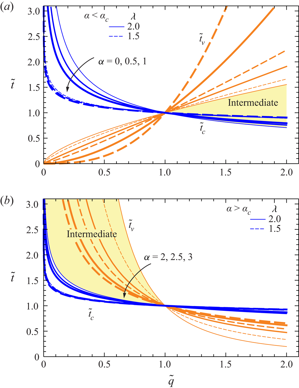
Figure 2. Evolution of the balance regime for a radial GC in the presence of vegetation as a function of the time exponent of the volume of denser fluid. (a) Diagrams for  $\alpha <\alpha _c\equiv (7\lambda -3)/(3\lambda +1)$ and (b) for $\alpha >\alpha _c$. The continuous curves refer to $\lambda =2$, while the dashed curves refer to $\lambda =1.5$. The hatched areas represent the domain where the intermediate asymptotic solution exists with turbulent drag–buoyancy balance; the intermediate asymptotic solution regime occurs after the initial phase, dominated by inertia, ending before the phase when viscosity is dominant.
Figure 2(b) shows the same data of figure 2(a) for  $\alpha >\alpha _c$, with the hatched area referring to $\alpha =2$ and $\lambda =2$. The intermediate asymptotic similarity solution is allowed only for $\tilde {q}<1$, the domain of existence becomes smaller for increasing $\alpha >\alpha _c$.
This analysis is approximate because it refers to homogeneous and invariant assumptions for  $h$,
$h$,  $u$ and for $\lambda$, $\tilde {c}$, which in real GCs are variable in space and time. In particular, near the front the current is always in the viscous–buoyancy balance regime. However, it provides useful insights to the discussion of the deviations of the theoretical model from experiments and to framing of the validity limits of a self-similar solution.
2.4. Solution
When  $\tilde {c}$ and $\lambda$ are constant and the volume is of the form $\mathcal {V} = q t^\alpha$ (including the fixed-volume LR case $\alpha = 0$) analytical solutions of similarity type can be obtained, as follows.
Let  $y = r/r_N(t)$. The equations of motion can be expressed in terms of the variables $h(y,t)$ and $u(y,t$). The domain of solution is $y \in [0,1]$ and the nose of the current is at $y=1$. We seek a similarity solution of the form
 \begin{equation} r_N = \mathcal{K} t^\gamma, \quad h = t^\delta \mathcal{H}(y), \quad u = \dot{r}_N \mathcal{U}(y), \end{equation}
where the upper dot denotes time derivative and  $\mathcal {K}, \gamma, \delta$ are constants. The task is to obtain the values of $\mathcal {K}, \gamma, \delta$ and the profiles $\tilde {\mathcal {H}}(y), \mathcal {U}(y)$ subject to the boundary conditions. The boundary conditions at the nose ( $y = 1$) are $\mathcal {U}(1) = 1, \mathcal {H}(1) = 0$. The global volume balance (per radian) is
 \begin{equation} \mathcal{V} = \int_0^{r_N} h r\,\textrm{d}r = \mathcal{K}^2t^{2\gamma} t^\delta\int_0^1 \mathcal{H}(y) y \,\textrm{d} y = q t ^{\alpha}; \end{equation}
and yields
 \begin{equation} 2 \gamma + \delta = \alpha; \quad \mathcal{K}^2 J = q, \end{equation}
where  $J = \int _0^1 \mathcal {H}(y) y \,\textrm {d} y$.
Substitution of the similarity form (2.21a–c) into the momentum equation (2.5) yields, after some algebra
 $$\begin{gather} \delta ={-} \lambda + \gamma (\lambda + 1); \end{gather}$$
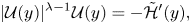 $$\begin{gather}|\mathcal{U}(y)|^{\lambda-1}\mathcal{U}(y) ={-}\tilde{\mathcal{H}}'(y) , \end{gather}$$
where
 \begin{equation} \tilde{\mathcal{H}}(y) = \frac{ \mathcal{H}(y)}{C}; \quad C = \frac{\tilde{c}}{g^{\prime}} \gamma ^\lambda \mathcal{K}^{1 + \lambda}. \end{equation}
Combining (2.23a,b) with (2.24) we find
 \begin{equation} \gamma = \frac{\alpha + \lambda}{3 + \lambda}. \end{equation}
The continuity equation reads
 \begin{equation} \frac{\delta}{\gamma} \, \tilde{\mathcal{H}}(y) + (\mathcal{U} - y) \tilde{\mathcal{H}}'(y) + \tilde{\mathcal{H}}(y) \mathcal{U}'(y) ={-} \frac{\mathcal{U}}{y} \tilde{\mathcal{H}}(y). \end{equation}
 For given  $\lambda$ and $\alpha$ we obtain $\gamma$ and $\delta$ by (2.27) and (2.24), then solve (2.25) and (2.28). Note that $\mathcal {U}(y)$ and $\tilde {\mathcal {H}}(y)$ are dimensionless. An analytical solution of (2.25) and (2.28) can be obtained for $\delta /\gamma = -2$
 \begin{equation} \mathcal{U} =y; \quad \tilde{\mathcal{H}}(y) = \frac{1}{1+ \lambda} (1 - y^{1+ \lambda}). \end{equation}
This is valid when
 \begin{equation} \gamma = \frac{\lambda}{3 + \lambda}; \quad \delta ={-}2 \gamma; \quad \alpha = 0. \end{equation}
 The validity of this result can be verified by direct substitution into the equations of motion, and it is evident that the boundary conditions  $\mathcal {U}(0) = 0, \tilde {\mathcal {H}}(1) =0$ are satisfied. This describes the propagation of a GC of fixed volume.
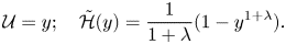
For influx values of  $\alpha >0$ the similarity profiles can be calculated by numerical integration. Typical results are shown in figure 3. We recall that the solution is irrelevant for small $y$, because a realistic source must have a finite radius. On the other hand, the solution is well behaved about the nose. Using an expansion in powers of $1-y$, we find that for small values of $1-y$ the solution of (2.25) and (2.28) can be approximated by
 \begin{equation} \tilde{\mathcal{H}} = (1-y) + \lambda \frac{\delta}{4 \gamma }(1-y)^2 + \cdots, \quad \mathcal{U} = 1 + \frac{\delta}{2 \gamma }(1-y) + \cdots . \end{equation}
Consequently, for given  $\alpha$ and $\lambda$ we calculate the profiles $\mathcal {U}(y), \, \tilde {\mathcal {H}}(y)$ by numerical integration from $y = 1- \varDelta$ to smaller values of $y$. Here, $\varDelta$ is some small interval which allows the application of the approximation (2.31a,b) as the initial condition for the integration, thus avoiding the problem of the zero coefficient of $\mathcal {U}'(1)$ in (2.28).
Figure 3. Theoretical profiles (a)  $\tilde {\mathcal {H}}$ and (b) $\mathcal {U}$ as functions of $y$ for $\alpha = 0.5 \text {--} 3$, $\lambda = 1$ (dotted lines) and $\lambda = 2$ (solid lines).
For  $\alpha = 3$ we find $\gamma = \delta = 1$ independent of $\lambda$; the aspect ratio of the current does not change with $t$. Typical solutions with influx conditions relevant to the present investigation are illustrated in figure 3.
The front position in dimensional variables is
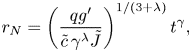 \begin{equation} r_N=\left(\dfrac{qg^{\prime}}{\tilde{c}\,\gamma^{\lambda}\tilde{J}}\right)^{1/(3+\lambda)}t^{\gamma}, \end{equation}
where  $\tilde {J}=\int _0^1\tilde {\mathcal {H}}(y)y\,\textrm {d} y$, which for $\alpha =0$ becomes
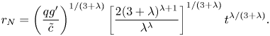 \begin{equation} r_N=\left(\dfrac{qg^{\prime}}{\tilde{c}}\right)^{1/(3+\lambda)}\left[\dfrac{2(3+\lambda)^{\lambda+1}}{\lambda^{\lambda}}\right]^{1/(3+\lambda)}t^{\lambda/(3+\lambda)}. \end{equation}
 Figure 4 shows the numerical value of  $\tilde {J}$ for different $\alpha$ and $\lambda$.
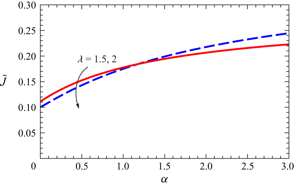
Figure 4. Value of the integral  $\tilde {J}$ as a function of $\alpha$ for $\lambda =1.5,2$.
3. The experimental layout and procedures
3.1. Set-up for the GCs
We ran a series of experiments at the Hydraulic Laboratory of the University of Parma. Our tank was a poly-methyl-methacrylate circular sector, with a radius of  $R = 180 \ \mathrm {cm}$ and an angle $\beta = 30^{\circ }$ as sketched in figure 5(a). The vegetation was modelled by (i) 200 vertical plastic rods, with a density $\kappa = 0.050$, as sketched in figure 5(a), and (ii) 320 rods, with a density $\kappa = 0.081$. The rods, with diameter $D = 1.6$ cm, were positioned according to an equilateral triangular mesh grid, with the edge of the triangles equal to 5.6 cm for $\kappa = 0.050$ and 5.0 cm for $\kappa = 0.081$.
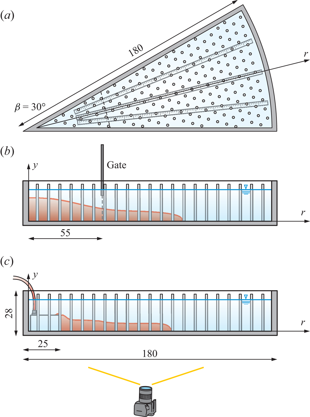
Figure 5. Experimental set-up with  $\kappa = 0.050$. (a) Top view; (b) lateral view of a LR experiment; and (c) lateral view of a continuous flux experiment. Units are in centimetres. Images are not corrected for distortion.
For the LR experiments, a stainless steel planar gate 0.2 cm thick was positioned at  $r_0 = 55 \ \mathrm {cm}$ and manually lifted just before the start of the experiment, see figure 5(b). The opening of the gate took approximately 0.2 s, a negligible time when compared with the duration of the experiments, $t = 40\text {--}60 \ \mathrm {s}$. A criterion for establishing the maximum gate opening time was formulated by Lauber & Hager (Reference Lauber and Hager1998) for dam breaks on a dry horizontal bottom with a vertical lift gate: if the opening occurs in a time greater than $t_{min}=\sqrt {2h_0/g^{\prime }}$, the initial flow field is distorted by the presence of the flat gate surface, increasing the discrepancy between theory and experiments. Applying this criterion, the critical condition for this experimental activity corresponds to $t_{min}=0.8\ \textrm {s}$, more than the opening time of 0.2 s for the present experiments.
For the experiments with a continuous source of flux, a home-made diffuser was inserted at  $r_0 = 25 \ \mathrm {cm}$, see figure 5(c). The diffuser was connected to a pump controlled in feedback by a LabView software. Different experiments were conducted with a constant, waxing or waning volume inflow rate.
The lateral view of the experiments was recorded by a full HD video-camera ( $1920\ \textrm {pixels} \times 1080\ \textrm {pixels}$, iPhone 7, Apple Inc.), working at 30 frames per second (fps). A 5 cm square grid stuck on the inner side of the front lateral wall was used to convert pixels into laboratory coordinates, with the aid of a proprietary Matlab code. The algorithm preliminary requires (i) the acquisition of the pixels of the knots of the grid; (ii) the computation of a conversion polynomial function for the two horizontal and vertical directions, mapping pixels into laboratory coordinates. The order of the polynomial is automatically chosen to minimize the root-mean-square deviation between the grid knots in laboratory coordinates and the reconstructed values starting from the pixels in the image. The conversion polynomials allow us to compensate for defects in the optics and for the position of the camera (Longo et al. Reference Longo, Ungarish, Di Federico, Chiapponi and Maranzoni2015, Reference Longo, Ungarish, Di Federico, Chiapponi and Addona2016), and are used to transform the pixels corresponding to the instantaneous profile of the current into laboratory coordinates.
The top view was recorded by a 4 k video camera (3840 pixels  $\times$ 2160 pixels, iPhone 11, Apple Inc.), working at 30 fps. The time evolution of the position of the nose of the current was measured by means of three radial grids glued at the base of the tank. High-frequency neon lamps provided stable and homogeneous illumination at the back wall of the tank. Softened tap water, with density $\rho _a = 1000 \ \mathrm {kg}\ \mathrm {m}^{{-3}}$, was always used as ambient fluid, although sometimes $\rho _a = 1001 \text {--}1002 \ \mathrm {kg}\ \mathrm {m}^{-3}$ because of salty traces left from previous experiments. The dense current was made of tap water, sodium chloride (NaCl) and red aniline dye, well mixed before the use.
For practical reasons, the fixed top condition is replaced by the free-surface condition, with no lid on the top of the tank. There is theoretical and experimental evidence that for Boussinesq systems (as considered in this paper) the difference between fixed and open top has negligible influence on the flow of the current, see Ungarish (Reference Ungarish2020).
In order to have an estimate of the mixing between the current and the ambient, some samples of the dense fluid were collected during some of the experiments listed in table 1, at the bottom of the current and a few millimetres below the interface, at  $r = 90$, 170, 175 cm. The samples were manually collected with a syringe connected to a 2 mm brass pipe, and then analysed with a refractometer.
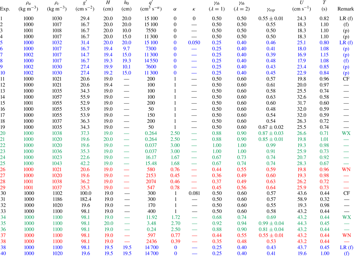
Table 1. Parameters of the experiments with rods of diameter  $D=1.6\ \textrm {cm}$: $\rho _{a,c}$ is the density of the ambient/current fluid, $g^{\prime }$ is the reduced gravity, $H$ is the initial height of the ambient fluid, $h_0$ is the height of the current in the LR experiments, $q'\equiv q(1-\kappa )$ is the inflow rate coefficient referring to the $30^\circ$ sector tank, $\kappa$ is the density of vegetation, $\alpha$ and $\gamma$ are constants; $\gamma _{th}$ is the theoretical value evaluated for $\lambda = 1, 2$, while $\gamma _{exp}$ is the experimental value; $U = \sqrt {g^{\prime } H}$ is the velocity scale, $T = H/U$ is the time scale. The abbreviations in the ‘Remark’ column stand for LR, LR full depth/partial depth (f/p), constant inflow rate (CF), waxing (WX) and waning (WN) inflow rate, respectively. Note that, in the comparison between experiments and theory, the fact that the volume in (2.26) includes both fluid and vegetation has been taken into account.
Appendix A describes further experiments for measuring the drag coefficient of a set of rods, in the same configuration adopted for the GC experiments.
3.2. The uncertainty in variables and parameters
We considered the instrument accuracy and the sequence of operations during tests to estimate the uncertainty of the variables and parameters. Hydrometers with an accuracy of  $10^{-3}\ \mathrm {g}\ \mathrm {cm}^{-3}$ were used to measure density, hence the corresponding uncertainty for the reduced gravity $g^{\prime } = (1-\rho _a/\rho _c)g$ is $\Delta g^{\prime }/g^{\prime } \le 0.2\,\%$. The level of the dense fluid in the lock and the level of the ambient fluid were measured by a ruler with an accuracy of $0.2\ \textrm {cm}$. The relative uncertainty is $\Delta h_0/h_0 \le 2\,\%$. The volumetric flow rate of the pump was controlled within 1 % of accuracy.
The Reynolds number of the current has an uncertainty  $\Delta Re/Re \le 4\,\%$, also based on the assumption of an uncertainty of $1\,\%$ in estimating the kinematic viscosity of salty water. The resolution in grabbing the lateral profiles of the dense current is approximately 0.1 cm pixel $^{-1}$, while the overall uncertainty due to parallax errors is approximately 0.3 cm.
The velocity of water during drag coefficient measurements has an uncertainty  $\Delta V/V = 2\,\%$ at high inflow rates and $\Delta V/V = 4\,\%$ at low inflow rates. Reynolds number of the vegetation has an uncertainty $\Delta Re_{{rod}}/Re_{{rod}} \le 6\,\%$ and the arrangement for measuring the drag force gives results with an uncertainty less than 10 %.
The inflow produces an increase of the level of the ambient fluid. The underlying idea of the thin-layer model is that the vertical velocity is much smaller than the horizontal velocity,  $w\ll u$. If we consider a constant inflow rate $q$, the rate of increase of level can be expressed as $w=2q/(\beta R^2),\beta =30^\circ$, which for the largest value $q=400\ \textrm {cm}^3\ \textrm {s}^{-1}$ of our experiments (exp. 33 in table 1) results in $w=0.04\ \textrm {cm}\ \textrm {s}^{-1}$, compared with a typical radial speed of $u=10\ \textrm {cm}\ \textrm {s}^{-1}$, hence the condition $w\ll u$ is satisfied. Over 25 s of experiment, the variation of the ambient fluid level equals $\Delta H=1\ \textrm {cm}$, representing 5.2 % of the initial ambient fluid $H=19\ \textrm {cm}$. This value is reached at the end of the experiment, and on average, $\Delta H/H=2.6\,\%$ which is in the range of the other experimental errors. In most of the other experiments $\Delta H/H$ is much smaller because $q$ is smaller and even null for LR experiments.
4. The experiments
Table 1 lists the parameters of the experiments. Experiments 1–4 were in a LR configuration and with no vegetation  $\kappa = 0$, in order to check the overall quality of the set-up in a simple configuration, without the effects of the rods. Experiments 5–29 were with a vegetation density of $\kappa = 0.050$, experiments 5–10 were LR while experiments 11–29 involved a continuous source of flux, constant or time varying. Finally, experiments 30–40 were with a vegetation density of $\kappa = 0.081$ and a constant source of flux.
Figure 6 shows some snapshots of the lateral view of the tank taken at  $t = 0, 4, 8$ and 16 s after the lift of the gate, during exp. 8 in LR, in order to give an overview of the shape of the current propagating radially from the centre. The dense current is red, while the ambient fluid is transparent. The vertical rods tend to overshadow the view, especially on the right-hand side of the images, where the radial distance $r$ is great and the number of rods filling the tank increases. The red colour of the dense current is also not homogeneous, as it gets darker from left to right as the gap of the tank increases from the centre towards the outer radius. In figure 6(a), at $t = 0$, the fluid is still at rest inside the lock, but as the gate is lifted, the current starts spreading and its thickness reduces in time. At a short time after the lift of the gate, a significant entrainment of the ambient fluid occurs as the current propagates, as we can see from figure 6(b), where the lock is still entirely filled by red fluid, but the nose of the current is advancing further. As time goes by, diffusion also occurs at the interface, and the dye appears stratified in concentration in the vertical direction, especially close to the left hand-side of the snapshots, at $r=0$, see figure 6(c,d). The red spot on the right-hand side in figure 6(d) is a reflection of the current on the transverse vertical wall.
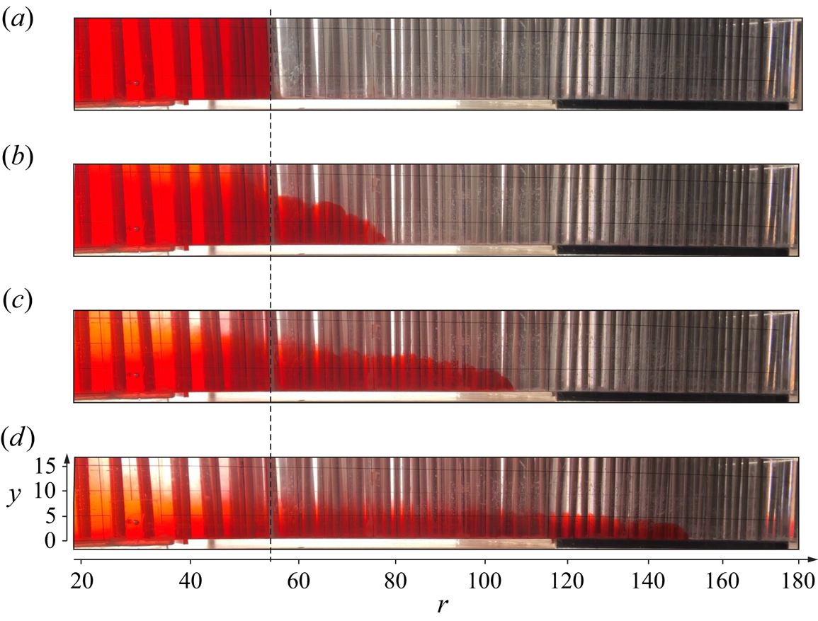
Figure 6. (a–d) Snapshots of the lateral side of the tank taken at  $t = 0, 4, 8$ and 16 s for exp. 8, LR ( $\alpha =0$). The dashed vertical line indicates the section of the gate. Units are in centimetres. The images are not corrected for distortion.
We observe that the condition  $h/H\ll 1$ is not strictly satisfied. It is indeed possible to develop more sophisticated models with two layers, but the mathematical complication (even in Cartesian cases, and much more so in a cylindrical geometry) usually prevents an intuitive solution. There is consensus in the research community that the one-layer model is a valid approximation tool for $h/H < 0.5$, although precise estimates of the magnitude of the error are not available (this is discussed in Ungarish Reference Ungarish2020).
Figure 7 shows some snapshots of the lateral view of the tank taken at  $t = 6, 36, 50$ and 60 s from the time when the pump was switched on, during exp. 22. In this experiment, the volume inflow rate increases with $Q \propto t^2$, and as $Q$ increases, the height of the current close to the source increases, with more evident billows.
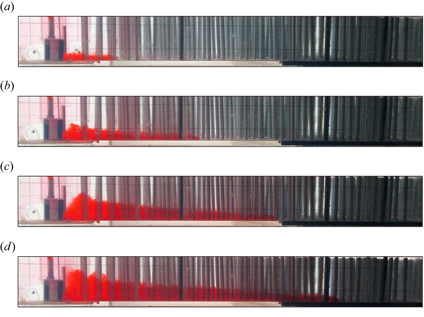
Figure 7. (a–d) Snapshots of the lateral side of the tank taken at  $t = 6, 36, 50$ and 60 s for exp. 22 ( $\alpha =3$), waxing inflow rate with $Q\propto t^2$. Images are not corrected for distortion.
Figure 8 represents snapshots of exp. 22 from the top. We can observe that the front of the current is fairly radially symmetric.

Figure 8. (a–d) Snapshots of the top view of the tank taken at the same times as figure 7,  $t = 6, 36, 50$ and 60 s during exp. 22 ( $\alpha =3$), waxing inflow rate with $Q\propto t^2$. Images are not corrected for distortion.
In order to gain further insights into the dynamics of these GCs, lateral profiles have been extracted at different times and for different kinds of inflow. Figure 9 shows some dimensional lateral profiles of the current taken at various instants, for an LR experiment (exp. 5) in figure 9(a), an increasing influx experiment (exp. 21) in figure 9(b), a decreasing influx experiment (exp. 28) in figure 9(c) and a constant influx experiment (exp. 33) in figure 9(d). In figure 9(a), the grey dotted vertical line at  $r = 55$ cm marks the position of the gate at $t =0$, while the grey dotted square at $r = 25$ cm in the other three panels is a schematic for the diffuser, so no data are available for $r < 25$ cm as the current only propagates downstream.
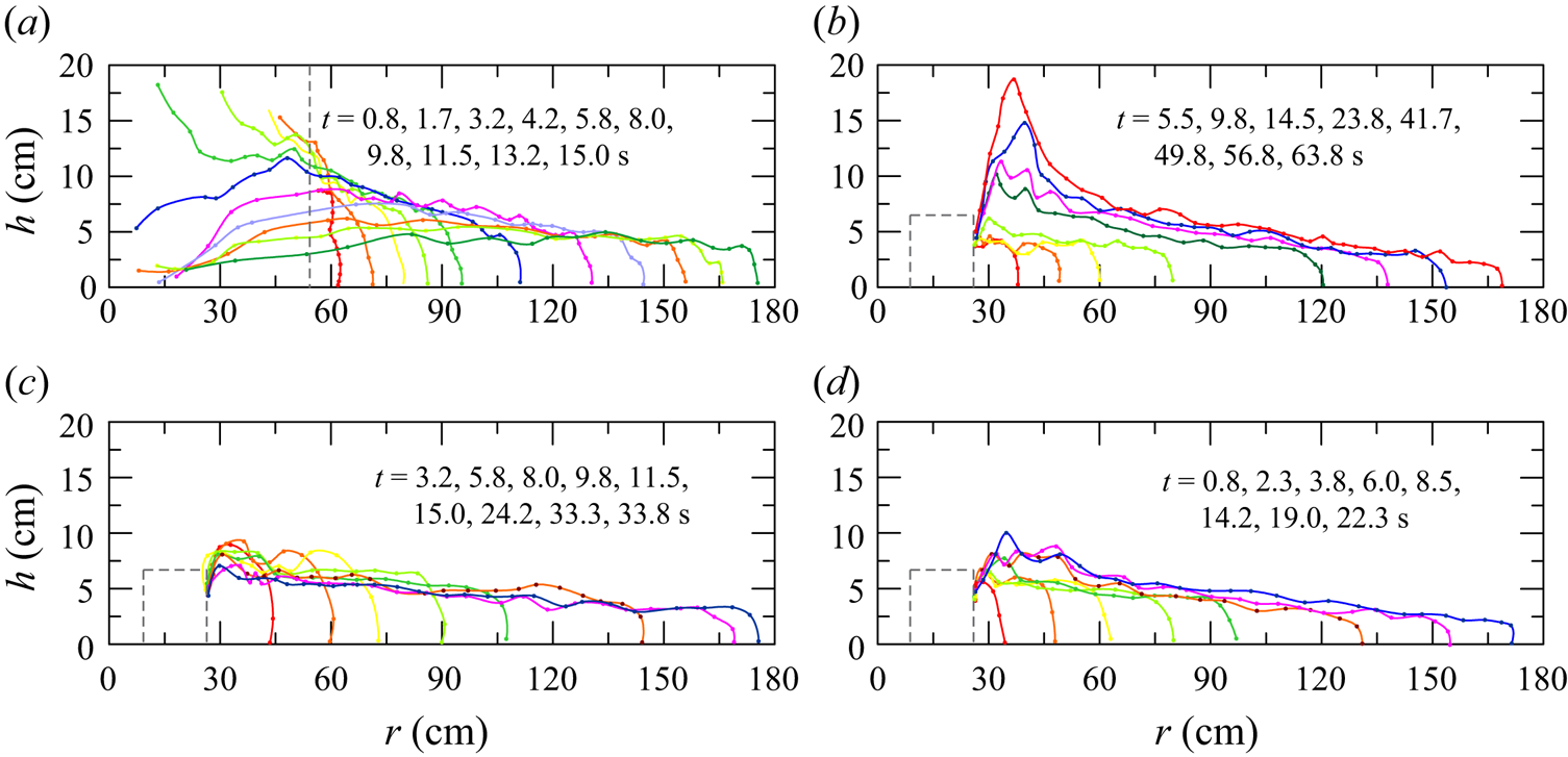
Figure 9. Dimensional lateral profiles extracted from images at various instants for (a) an LR experiment (exp. 5,  $\alpha =0$); (b) waxing influx experiment (exp. 21, $\alpha =2.5$); (c) waning influx experiment (exp. 28, $\alpha =0.46$); (d) constant influx experiment (exp. 33, $\alpha =1$).
Profile trends are consistent with expectations in all four reported cases. In the proximity of the fluid injection section (which in the experiments is necessarily advanced with respect to the origin of the cylindrical sector) the greatest deviations from the profiles, consistent with the shallow-water scheme of the analytical reference model, are observed. In the case of LR (figure 9a), the initial acceleration is sufficiently significant to make the inertial contribution dominant with respect to the drag of the vegetation. However, the decay of the inertial stage is fast due to the effect of vegetation and also because of the interaction with the ambient fluid, which in the region of the lock has a significant velocity and opposite to that of the current: it results in a very high shear with the formation of billows and entrainment of ambient fluid, and a consequent mixing.
As the front advances toward the periphery of the circular sector, the fluctuations at the interface between the dense current and the ambient fluid are damped, as the current front widens and the average velocity is reduced. The thickness of the current is reduced, and the dynamics appears more adherent to that of the interpretative model. An important difference, due to the presence of vegetation, is the scale of the turbulence, which is necessarily controlled also by the downstream wake of the cylinders. The mixing processes appear amplified, and consequently the interface between dense current and ambient fluid is less defined than in the case of the absence of vegetation.
For GCs with increasing flow rate over time (figure 9b), near the inlet section the turbulence level increases over time, creating an accumulation of denser fluid that originates a progressively increasing pressure gradient. The region with very different characteristics of the flow field and of the current, compared with the theoretical model, becomes progressively larger, even if the current, moving away from this region, appears to follow the theoretical model hypotheses. On the contrary, in the case of current with waning flow rate (figure 9c), the flow characteristics appear sufficiently smooth, with a progressive reduction, in time, of the thickness near the inlet section.
Last, currents generated by a constant inflow rate (figure 9d) reach a substantial equilibrium after a short time, with a current profile that, while fluctuating, remains essentially unchanged over time and with a modest reduction in the average interface slope.
By sampling in the vertical the dense current with a syringe, with the methodology described in § 3, we checked that the currents undergo a strong reduction in density while propagating, and are also stratified in the vertical direction. For example, in exp. 33, while  $\rho _c = 1100 \ \mathrm {kg}\ \mathrm {m}^{{-3}}$ in the container from where the pump takes fluid, the density decreases to $\rho _c = 1048 \pm 4 \ \mathrm {kg}\ \mathrm {m}^{{-3}}$ at the bottom and $\rho _c = 1033 \pm 3 \ \mathrm {kg}\ \mathrm {m}^{{-3}}$ just below the density interface. This is a result of a great entrainment of the light ambient fluid into the GC. The amount of entrainment was also evaluated by comparing the volume injected in the tank with the volume of the current estimated form the lateral profiles in time. We found that the volume estimated with the last technique was double the injected volume, almost uniformly during the current propagation. This dilution of the current by a factor of 2 was also found by Hatcher et al. (Reference Hatcher, Hogg and Woods2000), who stated that the mixing occurs for a few seconds after releasing the gate. They also suggest that the total buoyancy of the flow, given by the product of $g^{\prime } q$ is conserved during the flow, so if a reduction of $g^{\prime }$ occurs due to dilution, an increase in the value of $q$ compensates and the behaviour of the nose position is unaffected. We will verify this later on.
We now compare some experimental lateral profiles with the theoretical predictions in figure 10, where the theoretical height of current  $h$ is scaled with respect to a reference height $h_{ref}$, here set as $h_{ref}=h(y=0.2)$, and is shown as a function of the non-dimensional radial coordinate $y = r /r_N$. The choice of a reference section that differs, as would be natural, from the axis of the cylinder sector (i.e. with the origin of the chosen radial coordinate system), derives from the approximations of the physical model, which requires adequate space for the lock, or for the diffuser. From a mathematical point of view, the origin also generates a singularity. The results are little affected by the exact position of the reference section.
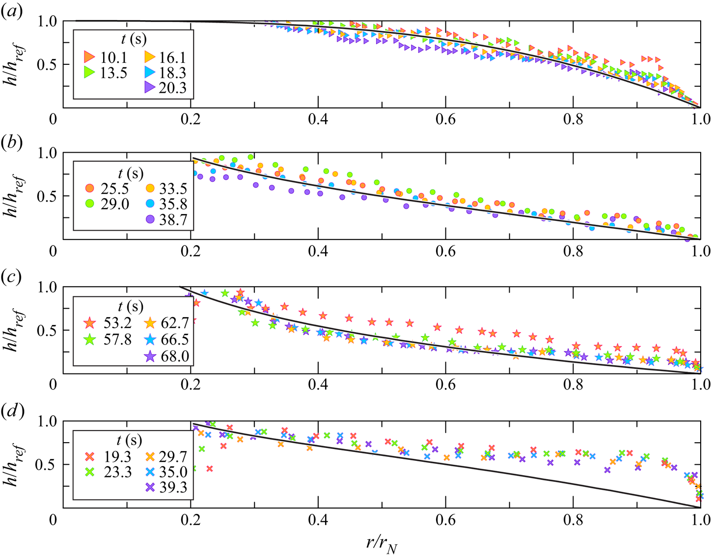
Figure 10. Lateral profiles of the current at different times for (a) a LR experiment,  $\alpha =0$, exp. $8$, (b) a constant inflow experiment, $\alpha =1$, exp. $17$, (c) a waxing inflow experiment, $\alpha =3$, exp. $22$ and (d) a waning inflow experiment, $\alpha =0.45$, exp. $27$. The solid black lines refer to the theoretical similarity solution, when $\lambda =2$ scaled with $h_{ref}$.
Figure 10(a) refers to an LR experiment ( $\alpha =0$, exp. $8$ in table 1), while figure 10(b–d) refers to constant inflow rate experiments (CF $\alpha =1$, exp. $17$), waxing inflow rate WX with $\alpha =3$, exp. $22$, and waning inflow rate $\alpha =0.45$, exp. $27$ in table 1 respectively). The vertical error bars are smaller than the size of the symbol and are not shown. The experimental and theoretical results show a variegated behaviour, especially at late times when the self-similar solution is reached. In figure 10(c), at $y = 0.2 \text {--}0.3$, the experimental data showing the engulfment of ambient fluid in the dense current at high $Q$, depart from the theoretical behaviour. This is consistent, as the SW model does not include mixing and entrainment. In addition, the nose of the current ( $y = 1$) has a shape different from the shape predicted by the theory. This is more evident when $\alpha = 3$, see figure 10(c), than for experiments with smaller $\alpha$, see figure 10(a,b). This can be attributed to viscosity, which becomes more relevant at low flow rates, with a corresponding lower front speed. The experimental front Reynolds number is systematically quite small. In figure 10(d), which refers to a waning inflow experiment, the experimental data differ significantly from the theoretical prediction, especially for $y > 0.5$. The first reason may stand in some technical issues related to the injection of fluid in the tank at early stage. The pump used in the present study works well between 20 and $500\ \mathrm {ml}\ \mathrm {s}^{-1}$, so a strong linear increase in the inflow rate was imposed by the LabView software for the first few seconds, in order to let the pump reach the full scale value. Then, the pump followed the fixed waning inflow rate law. This early strong injection may have led to a significant accumulation of fluid at the nose of the current. The thickness of the nose is then much larger than zero. Another reason for the difference between experimental data and theoretical predictions may stand in the radial extent of the tank, which could be insufficient for the self-similarity to be reached in the waning inflow rate conditions.
Figure 11 shows the time series of the non-dimensional position of the nose of current. The experiments are separated into three plots, and the experiments in each plot are separated into two–three groups for an easy visualization of the results. The data are subjected to a vertical shift, which has no influence on the slope of the fitting lines. The solid lines represent the theoretical slope  $\gamma = (\alpha + \lambda )/(3 + \lambda )$, evaluated for $\lambda = 2$.
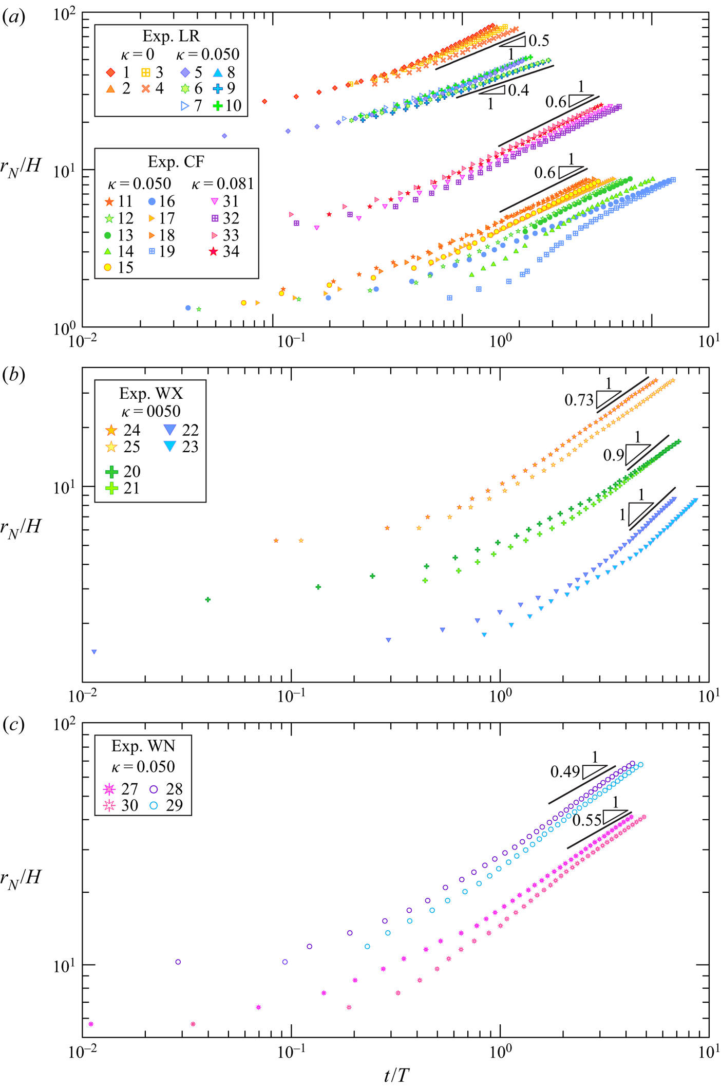
Figure 11. Non-dimensional position of the nose of the current as a function of the non-dimensional time (a) for LR experiments with  $\kappa = 0$ (LR exps 1–4), $\kappa = 0.050$ (LR exps 5–10), constant influx experiments with $\kappa = 0.050\text {--}0.081$ (CF exps 11–19 and CF exps 31–34); (b) for increasing influx (WX exps 20–25, $\kappa = 0.050$); and (c) for decreasing influx (WN exps 27–30, $\kappa = 0.050$). The slope of the black solid lines represents the theoretical power $\gamma$ computed for $\lambda =2$. The slope for exps 1–4 refers to the theoretical analysis in Ungarish (Reference Ungarish2009).
Figure 11(a) refers to the LR experiments without vegetation (exps 1–4,  $\kappa = 0$) and with vegetation (exps 5–10) and CF experiments with $\kappa = 0.050$ (exps 11–19) and $\kappa = 0.081$ (exps 31–34). Experiments without vegetation were run to check the overall quality of the experimental apparatus in a simple configuration. For all tests, the asymptotic trend appears significantly consistent with the theoretical slope, with varying times (lengths) of adaptation but with a remarkably large portion of the path characterized by linear trend (in log–log scale). This confirms that the front propagation is not affected by mixing and dilution of the current during propagation, as also suggested by Hatcher et al. (Reference Hatcher, Hogg and Woods2000). No appreciable difference is perceived as areal density of vegetation varies. The agreement is also for the four initial experiments without vegetation, where the exponent equals the theoretical value 0.5 as predicted in Ungarish (Reference Ungarish2009).
Figure 11(b) refers to increasing (waxing) inflow experiments (exps 20–25), where the different inclinations are related to various exponents of the inflow rate function. Again, the theory reproduces the experiments with adequate accuracy, although for exps 20–21 the asymptotic velocity is closer to the value that pertains to  $\lambda =1$ than to $\lambda =2$.
Figure 11(c) refers to decreasing (waning) inflow experiments (exps 27–30). In all four experiments, the front theoretical velocity is systematically below the experimental velocity. The experimental slope is around 0.6, 10 %–26 % greater than the theoretical values of 0.55–0.49 predicted when  $\alpha = 0.76 \text {--}0.45$ respectively. This modest agreement between theory and experiments was most visible in the side profiles. It is evident that the buoyancy of the GC appears to be influenced, starting from the profile near the front, by the secondary effects of mixing, resulting in an increase in apparent thickness and also in a different front velocity. A second possible reason, already mentioned before, is that the experimental apparatus is not long enough for the current to reach the self-similarity. We should note here that the self-similar solution requires an adjustment time and remains for a limited time, in the spirit of Barenblatt's self-intermediate asymptotic: in a first phase the system adjusts and gradually forgets the initial conditions; in a second phase it conforms to the self-similar solution; in a third phase it departs again from the self-similar condition because of perturbations that amplify, or because the assumptions of the model fail. In order for the solution obtained in turbulent drag–buoyancy balance to be applicable, it is also necessary that $t_{v1}< t< t_c$, as detailed in § 2.
The theoretical behaviour of the radial velocity  $u$ along the radial coordinate $r/r_N$ and computed for $\lambda =2$ is used to estimate the Reynolds number $Re = uh/\nu$ ( $h$ is the measured depth of the current, $\nu$ is the kinematic viscosity almost constant and equal to the fresh water value) shown in the left column in figure 12 for a LR experiment (LR exp. $5$) in panel (a), waxing influx experiment (WX exp. $21$) in panel (b), waning influx (WN exp. $28$) in panel (c) and constant influx (CF exp. $33$) in panel (d). Panels (e–h) in the right column refer to the same experiments and show the Reynolds number of the vegetation $Re_{{rod}} = ud/\nu$, where $u$ is the theoretical velocity of the current.

Figure 12. Profiles of the  $Re=uh/\nu$ (a–d) and $Re_{{rod}}=ud/\nu$ (e–h) against the radial coordinate $r/r_N$ for (a–e) LR experiment (exp. $5$,
$5$,  $\alpha =0$); (b–f) waxing influx (exp. $21$,
$21$,  $\alpha =2.5$); (c–g) waning influx (exp. $28$,
$28$,  $\alpha =0.46$); and (d–h) constant influx (exp. $33$,
$33$,  $\alpha =1$). Here, $Re$ is computed with $u$ from theory with $\lambda =2$ and $h$ from experiments, $Re_{{rod}}$ is computed with $u$ from theory with $\lambda =2$.
In all these plots, the value of  $\lambda =2$ has been assumed, but although the current is in a turbulent regime for much of its development, except near the front, the resistance of the vegetation is in general less than the expected one for $\lambda =2$, since $Re_{{rod}}$ is less than 3000. For LR experiments, the initial phase is characterized by fully developed turbulence of both the current scaled with its depth and scaled with the rods diameter. This behaviour reoccurs in a large portion of the current near the front, even in the later stages, while the turbulence decays and the resistance of the rods scales with $\lambda <2$ in the residual portion of the current, starting from the lock section. This justifies the good agreement of the theoretical model, which refers to a constant value of $\lambda$. In all other cases, although the value of the velocity remains fairly uniform with $r/r_N$, the level of turbulence of the current appears to be variable, and furthermore, on the basis of $Re_{{rod}}$, we expect a value of $\lambda <2$.
We observe that the front position is better reproduced by the model than the height profile of the currents. In fact, the front position scales with  $qg^{\prime }$, see (2.32), and the total buoyancy is preserved.
5. Conclusion
We experimentally studied the propagation of axially symmetric GCs in the presence of drag due to vegetation. A complementary part of the experimental work was concerned with the measurement of drag, which allowed us to estimate the  $\lambda$ exponent of the speed power law that expresses the drag on the propagation of the GC.
The exponent  $\lambda$ of the drag $\propto V^{\lambda }$ increases with $Re_{{rod}}$ and tends to 2 for $Re_{{rod}}\approx > 3000$. The transition is a function of $\kappa$, although the results of tests performed with only two values of this density cannot be sharp. Two additional sets of drag measurements with smaller diameter rods, with the same density, indicate that drag varies with $D$, with $\tilde {c}\propto (\kappa /D)^2$ and $\tilde {c}\propto (\kappa /D)$ for $\lambda =1,2$ for small $\kappa$; however, this variability only quantitatively affects the results, leaving unchanged the structure of the model, with the same asymptotic value for $\lambda$. Scaling drag measurements with the speed in the constricted section, instead of the apparent velocity, improves the collapse of drag coefficients to a unique universal value.
In order to analyse the variety of conditions under which the most dense fluid is injected, we conducted experiments with GCs produced by LR (constant volume), and also with GCs sustained by an influx that is either constant, increasing or decreasing in time. The analysis of the lateral profile of the current and the position of the front in time provide useful information for the classification of the pattern of the flow field. For all four cases, the current tends to become self-similar, with an asymptotic front speed that is reproduced quite well by a simple shallow-water one-layer model. In detail, the accuracy of the predictions is better for the LR tests, and is not so good for GCs sustained by waning flow rate. The reason is not the deficiency of the theoretical model, but rather the difficulty in specifying precisely the conditions at the influx position.
In order to obtain an estimate of the level of turbulence triggered by the floor of the tank and by the rods (this last one gives an estimate of the value of  $\lambda$), we calculated the Reynolds number of the current, with a geometric scale equal to the measured local depth, and the Reynolds number of the vegetation, with a geometric scale equal to the diameter of the rods. The current velocity was taken from the theoretical model. The result is that for LR the current is almost always turbulent and $Re_{{rod}}>3000$, i.e. $\lambda =2$; for the other tests the regime is viscous for more or less extended portions of the current and $Re_{{rod}}<3000$, without homogeneity. Such indications explain the experimental behaviour of currents, point to the causes of deviations from models and shed light on the more detailed aspects that deserve attention in more sophisticated models.
The theoretical analysis that predicts a self-similar flow and propagation with  $t$ at constant power, has been applied to currents that do not strictly or always meet the assumptions of the model, and hence the question of agreement and reliability is relevant. The experimental results indicate that some elements of self-similarity are still satisfied even if there are significant quantitative deviations in other aspects: the velocity of the current, for example, after an initial adaptation, becomes self-similar, but the experimental exponent in $r_N\sim t^\gamma$ is slightly different from the theoretical one; the differences can be attributed to the elements of the process that have not been deliberately included, first mixing and entrainment. Other variables, such as current depth, take on different values from the experiments (this is the case with waning flow rate currents), but the experiments still indicate a self-similar profile. We think that this is an encouraging insight of our experimental study. The theoretical model makes some bold simplifications, but it turns out that the associated effects make only a small contribution to the overall behaviour of the current. It is as if the self-similar solution is extremely stable even in the presence of strong disturbances, albeit with slightly different scaled variables than the theoretical model. This behaviour was already known and described with reference to the initial and boundary conditions, which are soon ‘forgotten’ by the current, reaching a self-similar regime sooner or later. (We note in passing that the attainment of self-similarity may be reached for some non-circular lock geometries, see Zgheib, Bonometti & Balachandar (Reference Zgheib, Bonometti and Balachandar2015), although without reaching axisymmetric shape and hence without forgetting the initial asymmetry).
As an extension of the analysis, the parameterization of mixing and entrainment processes and their involvement in the model is suggested. It is likely that the analytical structure leading to self-similarity of the first kind will be lost due to the introduction of new scales in the process. Something similar has already been addressed, for example in Hogg et al. (Reference Hogg, Ungarish and Huppert2000) and in Di Federico et al. (Reference Di Federico, Longo, King, Chiapponi, Petrolo and Ciriello2017), and solved with perturbation techniques. Possibly, a self-similarity of the second kind arises, where a power-law dependence of the variables is retained but with the exponents represented by eigenvalues of the differential problem.
Funding
The cost of the equipment used for this experimental investigation was partly supported by the University of Parma through the Scientific Instrumentation Upgrade Programme 2018. D.P. has been partly supported by the Programme ‘FIL 2019-Quota Incentivante’ of University of Parma and co-sponsored by Fondazione Cariparma. M.U. thanks the Dept. of Mechanical and Aerospace Engineering at Princeton University for supporting a visit in summer 2019, during which a part of this research was performed. We thank Professor H.A. Stone for interesting discussions of the problem. The authors thank master degree student N. Merli for his help in data acquisition and data analysis.
Declaration of interests
The authors report no conflict of interest.
Appendix A. Drag measurements for different rods diameter and scaling rules
An additional set-up was built in order to measure the drag coefficient of a set of rods, attached to a wooden panel, with density  $\kappa = 0.050 \text {--} 0.081$ and with two different diameters of the rods, arranged in order to keep constant the density while reducing the distance between two neighbouring rods. The drag analysis was extended beyond what was strictly necessary for the experimental study of the GCs in our experiments, in order to quantify the joint effect of density and diameter of the rods. The wooden panel with the rods was positioned inside a rectangular channel, as illustrated in figure 13. The channel was filled with water up to $h = 19.9$ cm, so that the rods were almost entirely immersed in the fluid. A tension load cell was put at the top of the panel in order to measure the drag force $F$ of the set of rods, when crossed by different values of volume inflow rates $Q$, hence by water flowing at different horizontal velocity $V$. The tension load cell was previously calibrated with a dynamometer with an accuracy of $0.01\ \textrm {N}$ in the same set-up configuration but in air. A spring slightly pulled the panel at the downstream side of the channel in order to apply a pre-tension to the load cell and let the measurements fall within the instrumental range of the dynamometer, eliminating the dead band.
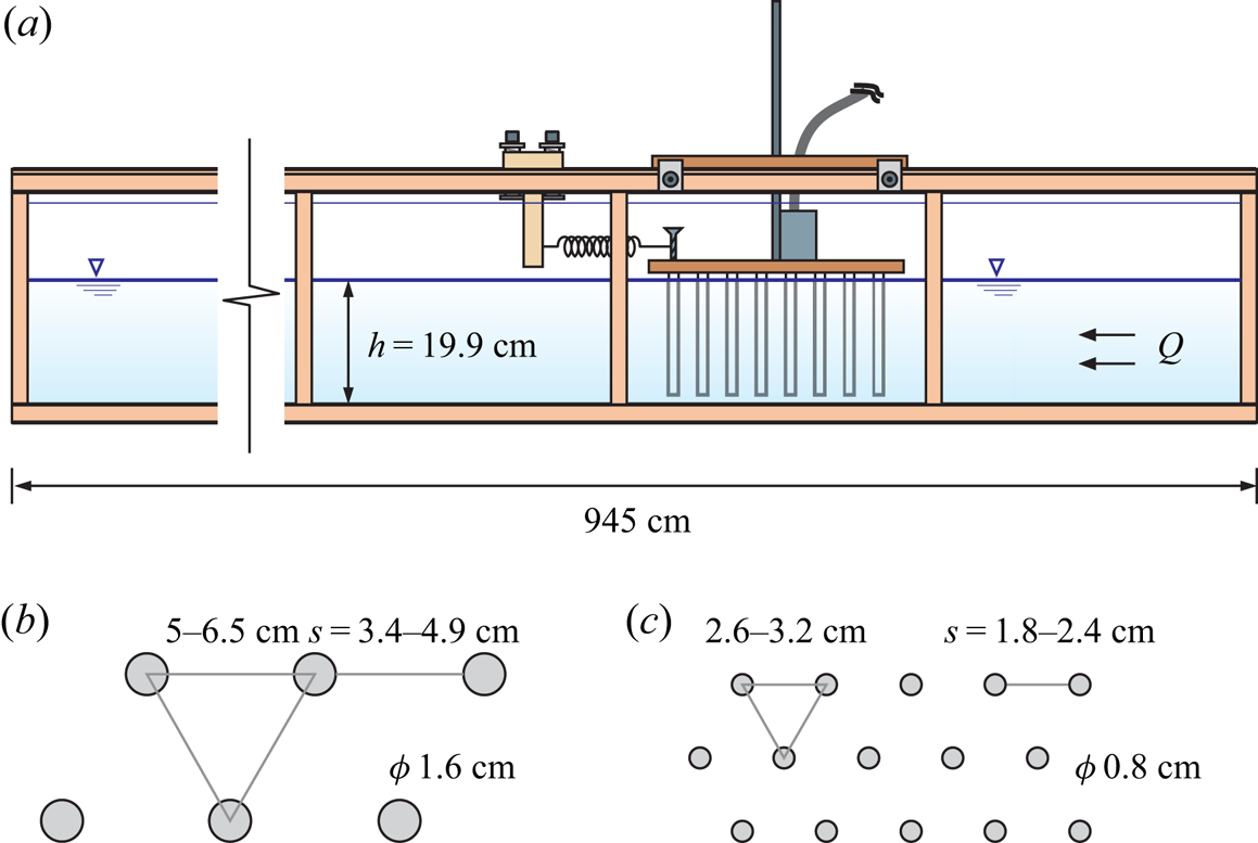
Figure 13. Experimental set-up for the drag measurement. (a) Side view of the channel with the panel supporting the rods and the load cell; (b) plan view of the 1.6 cm diameter rods; and (c) view of the 0.8 cm diameter rods.
Table 2 lists the main parameters of the two patterns with two different diameters of the rods for the drag force measurements, which for the diameter  $D=1.6\ \textrm {cm}$ correspond to the patterns adopted for the GC experiments documented in the main body of this manuscript.
Table 2. Arrangements of varying rod concentration and diameter  $D=1.6\text {--}0.8\ \textrm {cm}$. Here, $a$ is the frontal area per unit volume.
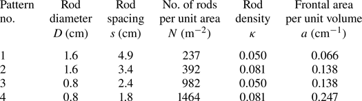
Figure 14(a,b) shows the drag force measurements as function of  $V$ (top axis) and of $Re_{{rod}}$ (bottom axis) for the set of rods with density $\kappa = 0.050$ and 0.081, respectively, and diameter 1.6 cm. The module of the drag force for a generic body can be expressed as
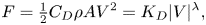 \begin{equation} F = \tfrac{1}{2} C_D \rho A V^{2} = K_D |V|^{\lambda}, \end{equation}
where  $C_D$ is the average drag coefficient, $\rho$ is the fluid density and $A$ is the frontal area of the body, $V$ is the apparent velocity (defined as the discharge in the rod layer over the gross cross-sectional area) and $Re_{{rod}} = V D / \nu$, where $D$ is the diameter of the rod and $\nu$ is the kinematic viscosity of water, assumed equal to $10^{-6}\ \textrm {m}^2\ \textrm {s}^{-1}$.

Figure 14. Drag measurements for 1.6 cm diameter rods. (a) Drag force  $F$ for $\kappa = 0.050$, and (b) for $\kappa = 0.081$ (the grey squares are a test of reproducibility of drag measurement after two months from the test visualized with blue triangles) and $\lambda$ refers to the right axis; (c) the drag coefficient $C_D$ as a function of the Reynolds number $Re_{{rod}}$, with different vertical axes for an easy visualization; (d) the drag coefficient as a function of $\lambda$. The dashed curves are the 95 % confidence limits, error bars indicate one standard deviation.
In our experiments,  $A = n A_r$, where $n = 36 \text {--} 55$ is the number of 1.6 cm diameter rods ( $n = 126 \text {--} 210$ for the 0.8 cm diameter rods) attached to the panel for $\kappa = 0.050 \text {--} 0.081$ respectively, and $A_r$ is the frontal area of a single rod covered by water, equal to $A_r=D\,l_s$ with $l_s$ the submerged length of the rod.
Figure 14(c) shows the drag coefficient as a function of  $Re_{{rod}}$, with vertical error bars computed by propagating in quadrature the uncertainties of the involved variables
 \begin{equation} \dfrac{\Delta C_D}{C_D}=\sqrt{\left(\dfrac{\Delta F}{F}\right)^2+\left(\dfrac{\Delta \rho}{\rho}\right)^2+\left(\dfrac{\Delta D}{D}\right)^2+\left(\dfrac{\Delta l_s}{l_s}\right)^2+4\left(\dfrac{\Delta V}{V}\right)^2}, \end{equation}
where  $l_s$ is the submerged height of the rods. The main contribution to uncertainty is due to velocity estimation and to force measurement. In fully turbulent flows, the drag coefficient is constant. On the other hand, in transitional and viscous regime the drag coefficient depends on the fluid velocity and on $\kappa$.
We can identify two different regimes where the drag force  ${\sim } V$ for $Re_{{rod}}<3000$ and ${\sim } V^2$ for $Re_{{rod}}>3000$. This is a classical result valid for internal and external flows, with the drag coefficient proportional to the inverse of the Reynolds number in the viscous regime, and independent of the Reynolds number in the asymptotic turbulent regime, at high Reynolds number (asymptotic independence of turbulence from viscosity). For the experiments with $\kappa =0.050$ the regression analysis of the experimental data for $D=1.6\ \textrm {cm}$ gives
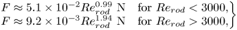 \begin{equation} \left.\begin{array}{ll@{}} F\approx5.1\times 10^{{-}2}Re_{{rod}}^{0.99}\ \textrm{N} & \textrm{for}\ Re_{{rod}}<3000,\\ F\approx 9.2\times 10^{{-}3}Re_{{rod}}^{1.94}\ \textrm{N} & \textrm{for}\ Re_{{rod}}>3000, \end{array}\right\} \end{equation}
respectively. The results are similar for  $\kappa =0.081$.
If we calculate the logarithm of (A1) and then differentiate, we obtain
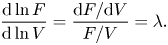 \begin{equation} \dfrac{\textrm{d}\ln F}{\textrm{d}\ln V} = \dfrac{\mathrm{d}F/\mathrm{d}V }{F/V}=\lambda. \end{equation}
 Figure 14(a,b) shows the values of  $\lambda$ (filled circles) referred to the right vertical axis. The regression functions are
 \begin{equation} \left.\begin{array}{ll@{}} \lambda=2-1.2\times 10^4Re_{{rod}}^{{-}1.5} & \textrm{for}\ \kappa =0.050,\\ \lambda=2-4.3\times 10^2 Re_{{rod}}^{{-}1} & \textrm{for}\ \kappa =0.081. \end{array}\right\} \end{equation}
 Figure 14(c) shows the drag coefficient  $C_D$ derived from (A1), as a function of $Re_{{rod}}$ for $\kappa = 0.050 \text {--} 0.081$, respectively. For both values of $\kappa$, we can observe a progressive transition towards the asymptotic drag coefficient. The interpolating curves are
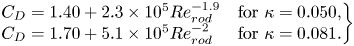 \begin{equation} \left.\begin{array}{ll@{}} C_D=1.40+2.3\times 10^5Re_{{rod}}^{{-}1.9} & \textrm{for}\ \kappa = 0.050, \\ C_D=1.70+5.1\times 10^5Re_{{rod}}^{{-}2} & \textrm{for}\ \kappa = 0.081. \end{array}\right\} \end{equation}
The drag increases with  $\kappa$ and assumes the asymptotic values $C_{D\infty } = 1.40 \pm 0.10$ and $C_{D\infty } = 1.70 \pm 0.10$, for $\kappa = 0.050 \text {--} 0.081$, respectively. Regarding the dependence of the drag coefficient on Reynolds number and, more generally, on the characteristics of the flow field and of the vegetation (Vargas-Luna et al. Reference Vargas-Luna, Crosato, Calvani and Uijttewaal2016) indicate that the drag of the vegetation is a function of other variables as well. In this respect, the structure of (A6) is an approximation. Figure 14(d) shows $C_D$ vs $\lambda$, with the drag coefficient decreasing linearly with the value of $\lambda$.
A similar analysis was conducted for rods with  $D=0.8\ \textrm {cm}$. The interpolating curves are
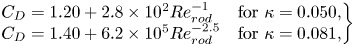 \begin{equation} \left.\begin{array}{ll@{}} C_D=1.20+2.8\times 10^2Re_{{rod}}^{{-}1} & \textrm{for}\ \kappa = 0.050, \\ C_D=1.40+6.2\times 10^5Re_{{rod}}^{{-}2.5} & \textrm{for}\ \kappa = 0.081, \end{array}\right\} \end{equation}
with asymptotic values  $C_{D\infty }=1.20\pm 0.10$ and $C_{D\infty }=1.40\pm 0.10$ for $\kappa =0.05\text {--}0.081$, respectively. These values are very similar to those calculated for rods of diameter 1.6 cm. Figure 15 shows $\lambda$ and $C_D$ as a function of $Re_{{rod}}$ for $\kappa = 0.050\text {--}0.081$ and for $D=1.6\text {--}0.8\ \textrm {cm}$.
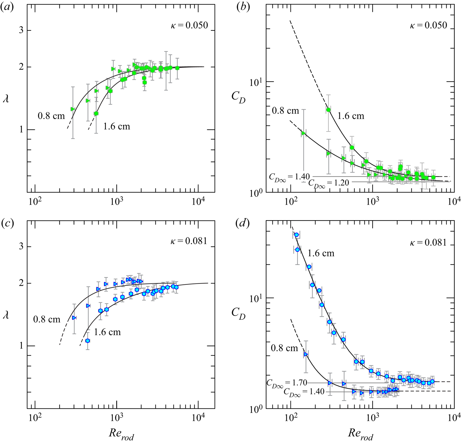
Figure 15. Comparison of drag measurements for 1.6 and 0.8 cm diameter rods. (a) Exponent  $\lambda$ and (b) drag coefficient for $\kappa =0.050$ as a function of $Re_{{rod}}$; (c,d) same variables for $\kappa =0.081$. Curves are the interpolating functions, error bars refer to one standard deviation.
From the definition results the drag contribution term is
 \begin{equation} \tilde{c}|V|^\lambda=\dfrac{F}{\rho b l l_s}, \end{equation}
where  $b$ is the channel width, $l$ is the streamwise length of the support of the rods and $l_s$ is the height of the rods, almost equal to the water depth. Figure 16(a,b) shows the experimental values and the interpolating curves of the coefficient $\tilde {c}$ and of $\lambda$.
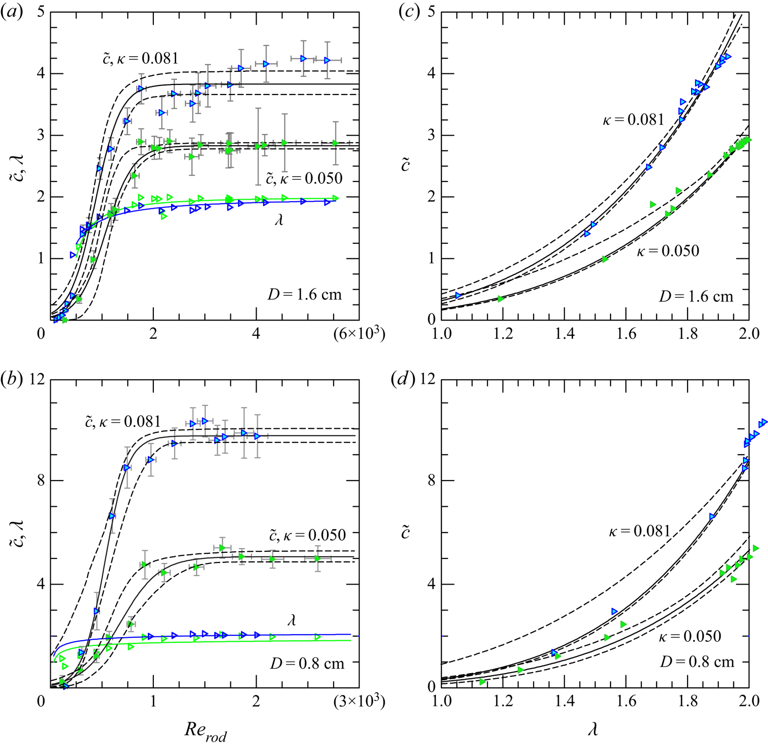
Figure 16. Drag measurements for 1.6 and 0.8 cm diameter rods. (a,b) Coefficient  $\tilde {c}$ (filled symbols) and $\lambda$ (open symbols) as a function of $Re_{{rod}}$ for $\kappa = 0.050\text {--}0.081$, and (c,d) coefficient $\tilde {c}$ as a function of $\lambda$ for $\kappa = 0.050\text {--}0.081$, with $\tilde {c}\propto \lambda ^{\approx 4}$. Curves are the interpolating functions; error bars and confidence bands refer to one standard deviation.
The interpolating functions for  $\tilde {c}$ are sigmoids with expression for $D=1.6\text {--}0.8\ \textrm {cm}$
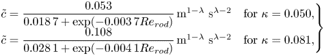 \begin{equation} \left.\begin{array}{ll@{}} \tilde{c}=\dfrac{0.053}{0.018\,7+\exp({-}0.003\,7Re_{{rod}})}\,\textrm{m}^{1-\lambda}\ \textrm{s}^{\lambda-2} & \textrm{for}\ \kappa = 0.050, \\ \tilde{c}=\dfrac{0.108}{0.028\,1+\exp({-}0.004\,1Re_{{rod}})}\,\textrm{m}^{1-\lambda}\ \textrm{s}^{\lambda-2} & \textrm{for}\ \kappa = 0.081, \end{array}\right\} \end{equation}
and
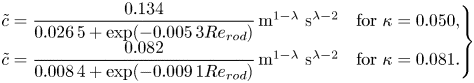 \begin{equation} \left.\begin{array}{ll@{}} \tilde{c}=\dfrac{0.134}{0.026\,5+\exp({-}0.005\,3Re_{{rod}})}\,\textrm{m}^{1-\lambda}\ \textrm{s}^{\lambda-2} & \textrm{for}\ \kappa = 0.050, \\ \tilde{c}=\dfrac{0.082}{0.008\,4+\exp({-}0.009\,1Re_{{rod}})}\,\textrm{m}^{1-\lambda}\ \textrm{s}^{\lambda-2} & \textrm{for}\ \kappa = 0.081. \end{array}\right\} \end{equation}
The asymptotic values corresponding to  $\lambda =1,2$ for $D=1.6\text {--}0.8\ \textrm {cm}$ are equal to
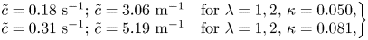 \begin{equation} \left.\begin{array}{ll@{}} \tilde{c}=0.18\ \textrm{s}^{{-}1};\,\tilde{c}=3.06\ \textrm{m}^{{-}1} & \textrm{for}\ \lambda=1,2,\,\kappa = 0.050, \\ \tilde{c}=0.31\ \textrm{s}^{{-}1};\,\tilde{c}=5.19\ \textrm{m}^{{-}1} & \textrm{for}\ \lambda=1,2,\,\kappa = 0.081, \end{array}\right\} \end{equation}
and
 \begin{equation} \left.\begin{array}{ll@{}} \tilde{c}=0.23\ \textrm{s}^{{-}1};\,\tilde{c}=5.34\ \textrm{m}^{{-}1} & \textrm{for}\ \lambda=1,2,\,\kappa = 0.050, \\ \tilde{c}=0.26\ \textrm{s}^{{-}1};\,\tilde{c}=8.84\ \textrm{m}^{{-}1} & \textrm{for}\ \lambda=1,2,\,\kappa = 0.081. \end{array}\right\} \end{equation}
Figure 16 shows the experimental values and the interpolating curves of the coefficient  $\tilde {c}$ and of $\lambda$.
Flow within the rods and porous structures is opposed by a viscous resisting force  $\propto V$ and form drag $\propto V|V|$, as derived from the Forchheimer equation (Whitaker Reference Whitaker1996); the former is a function of the permeability $K$, which is controlled by the internal geometry of the medium, the latter is a function of a dimensional drag coefficient $\chi$ controlled again by the internal geometry of the medium. In the present model, a single monotonic expression is adopted, with a resisting force $\propto V|V|^{\lambda -1}$ and $\lambda \in [1, 2]$. There are several models to relate $K$ and $\chi$ to the properties of the medium, and a scaling for drag can be obtained following the model proposed by Macdonald et al. (Reference Macdonald, El-Sayed, Mow and Dullien1979), who, on the basis of data from numerous experiments with a variety of materials, including cylinders, proposed a variant of the Ergun equations (Ergun Reference Ergun1952), with the permeability expressed as
 \begin{equation} K=\dfrac{D_{eq}^2(1-\kappa)^3}{a_0\kappa^2}\to \left.\tilde{c}\right|_{\lambda=1}=\dfrac{\nu(1-\kappa)}{K}\equiv \dfrac{a_0\nu\kappa^2}{D_{eq}^2(1-\kappa)^2}, \end{equation}
and the dimensional coefficient  $\chi$ expressed as
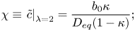 \begin{equation} \chi\equiv\left.\tilde{c}\right|_{\lambda=2}=\dfrac{b_0\kappa}{D_{eq}(1-\kappa)}; \end{equation} $a_0$ and $b_0$ are empirical constants and $D_{eq}$ is an equivalent mean sphere diameter ( $D_{eq}=6W_p/A_p$ being $W_p$ and $A_p$ the volume and the surface area of the particles) equal to $1.5D$ for a cylinder.
The scaling rules for  $\tilde {c}|_{\lambda =1}$ and for $\tilde {c}|_{\lambda =2}$ for small $\kappa$ are (Longo Reference Longo2022)
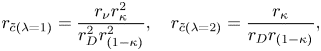 \begin{equation} r_{\tilde{c}(\lambda=1)}=\dfrac{r_{\nu}r_{\kappa}^2}{r_D^2r_{(1-\kappa)}^2},\quad r_{\tilde{c}(\lambda=2)}=\dfrac{r_{\kappa}}{r_Dr_{(1-\kappa)}}, \end{equation}
where  $r_{\nu }$, $r_{\tilde {c}}$, $r_{\kappa }$, $r_{(1-\kappa )}$ and $r_D$ are the ratios between the values of $\nu$, $\tilde {c}$, $\kappa$, $(1- \kappa )$ (the porosity) and $D$ of two different patterns.
Table 3 lists the experimental results of  $\tilde {c}$ for the four drag measurements tests with two different diameters and density of the rods. The values of the ratio $r_{\tilde {c}}$ are also listed as computed with the experimental data and with (A15a,b), with pattern number 1 assumed as reference. The agreement between theory and experiments is quite strong (differences within $15\,\%$) for the case $\lambda =2$, also considering that the agreement found by Macdonald et al. (Reference Macdonald, El-Sayed, Mow and Dullien1979) with (A13)–(A14) was within ${\pm }50\,\%$ for all the experimental data considered, if $a_0=180$ and $b_0=1.8$. The agreement for laminar flow is less evident, although the increment of $\tilde {c}$ with $\kappa$ is correctly reproduced. The latter discrepancy was expected, since the number of data and the accuracy of measurements in the viscous regime is lower than in the turbulent regime.
Table 3. Experimental values of  $\tilde {c}$ for the four drag measurements tests in the limiting cases of $\lambda =1,2$. There is a comparison between the experimental ratio $r_{\tilde {c}}-\exp$. and theoretical scaling $r_{\tilde {c}}-$theory indicated by (A15a,b), by assuming pattern no. 1 as reference and $r_{\nu }=1$.
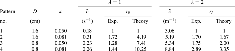
The relevant result for the present drag measurements is that the asymptotic value of  $\lambda$ is unaffected by the rods diameter, although the transitions from the viscous drag regime to the turbulent drag regime and drag values are affected. For small $\kappa$ it results that $\tilde {c}\propto (\kappa /D)^2$ and $\tilde {c}\propto (\kappa /D)$ for $\lambda =1,2$ respectively.
A more in-depth analysis aims to identify the appropriate variables to be adopted to express drag, towards a single expression valid for possible combinations of porosity and obstacle arrangement. Stone & Shen (Reference Stone and Shen2002) have suggested expressing the drag in terms of the average velocity at a constricted section,  $V_c$, in the rods, defined by Whitaker (Reference Whitaker1996) the ‘intrinsic average’ velocity as opposite to the ‘superficial average’ velocity. The velocity $V_c$ can be computed from the superficial velocity (defined as the discharge in the rod layer over the gross cross-sectional area) with the following equation (see Stone & Shen Reference Stone and Shen2002):
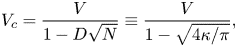 \begin{equation} V_c=\dfrac{V}{1-D\sqrt{N}}\equiv\dfrac{V}{1-\sqrt{4\kappa/{\rm \pi}}}, \end{equation}
where  $N$ is the number of rods per unit area. Figure 17 shows the same variables already presented in figure 15 but referred to $V_c$. The asymptotic values of the drag coefficients are more uniform than the data referred to the apparent velocity $V$, and have the same value for different densities, although still show a variability with the rods diameter.

Figure 17. Comparison of drag measurements for 1.6 and 0.8 cm diameter rods. (a) Exponent  $\lambda _c$ and (b) drag coefficient $C_{D,c}=2F/(\rho A V_c^2)$ for $\kappa =0.050$ as a function of $Re_{{rod,c}}=V_cD/\nu$; (c,d) same variables for $\kappa =0.081$. Curves are the interpolating functions, error bars refer to one standard deviation. Subscript ‘c’ refers the variables to data elaboration with $V_c$ instead of $V$.
$V$.
Appendix B. Scaling rules of the system
Our goal is to develop dynamic similarity criteria that allow to relate two realizations of the physical process we are analysing, but with different values of the variables or parameters involved: a first realization can be an experiment in the laboratory (model), a second realization can be the corresponding real GC in the field (prototype). We will make use of direct analysis, with similarity criteria developed on the basis of the two equations (2.5)–(2.6) that govern the process (see Longo Reference Longo2022).
Assuming a common vertical and radial geometric scale  $r_l$ (undistorted model), results in
 $$\begin{gather} r_{g'}=r_{\tilde{c}}r_u^{\lambda}, \end{gather}$$
 $$\begin{gather}r_l^3=r_qr_t^{\alpha}, \end{gather}$$
where  $r_{(\dots )}$ is the ratio between the value of the variable in the model and in the prototype
 \begin{equation} r_{(\dots)}=\dfrac{(\dots)_m}{(\dots)_p}. \end{equation}
The subscripts ‘m’ and ‘p’ stand for model and prototype, respectively.
Using the scaling rules (A15a,b), (B1a) reduces to
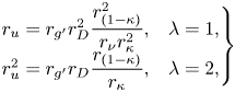 \begin{equation}
\left. \begin{array}{ll@{}}
r_u=r_{g'}r_{D}^2\dfrac{r_{(1-\kappa)}^2}{r_{\nu}r_{\kappa}^2},
& \lambda=1,\\
r_u^2=r_{g'}r_D\dfrac{r_{(1-\kappa)}}{r_{\kappa}}, &
\lambda=2, \end{array}\right\}
\end{equation}
\begin{equation}
\left. \begin{array}{ll@{}}
r_u=r_{g'}r_{D}^2\dfrac{r_{(1-\kappa)}^2}{r_{\nu}r_{\kappa}^2},
& \lambda=1,\\
r_u^2=r_{g'}r_D\dfrac{r_{(1-\kappa)}}{r_{\kappa}}, &
\lambda=2, \end{array}\right\}
\end{equation}In (B3b) a classical Froude similarity is achieved, where the geometric scale is related to the stem diameter.
Equation (B1b) becomes
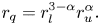 \begin{equation} r_q=r_l^{3-\alpha}r_u^{\alpha}. \end{equation}
We have two equations in eight variables, represented by the scale ratios
 \begin{equation} r_u,\quad r_q,\quad r_l,\quad r_{g'},\quad r_D,\quad r_{(1-\kappa)},\quad r_{\kappa},\;r_{\nu}, \end{equation}
with 6 degrees of freedom: for instance fixing  $r_l,r_{g'},r_D,r_{(1-\kappa )},r_{\kappa },r_{\nu }$ we can estimate $r_u,r_q$ and the scale ratios for all the derived variables. We can select the scale ratios almost arbitrarily, as long as the two realizations of the physical process both satisfy the basic assumptions (shallow-water equation, Boussinesq hypothesis, etc.) and $Re$ and $Re_{rod}$ take values in the range of validity of those assumptions. Table 4 lists the similarity rules computed for $\lambda =1,2$, undistorted model.
Table 4. Similarity ratios computed for the two cases  $\lambda =1$ and $\lambda =2$, undistorted model.
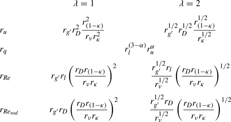
Since the GCs we are studying can be very large in plan, it can be advantageous to make geometrically distorted models with a vertical scale larger than the horizontal scale. For geometrically distorted models, defining  $r_{l_{h}}$ and $r_{l_{v}}=nr_{l_{h}}$ the horizontal and vertical length scale ratios, respectively, and $n$ the distortion coefficient (in general $n>1$), (B3) become
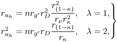 \begin{equation}
\left. \begin{array}{@{}ll@{}}
r_{u_{h}}=nr_{g'}r_{D}^2\dfrac{r_{(1-\kappa)}^2}{r_{\nu}r_{\kappa}^2},
& \lambda=1,\\
r_{u_{h}}^2=nr_{g'}r_D\dfrac{r_{(1-\kappa)}}{r_{\kappa}}, &
\lambda=2, \end{array}\right\}
\end{equation}
\begin{equation}
\left. \begin{array}{@{}ll@{}}
r_{u_{h}}=nr_{g'}r_{D}^2\dfrac{r_{(1-\kappa)}^2}{r_{\nu}r_{\kappa}^2},
& \lambda=1,\\
r_{u_{h}}^2=nr_{g'}r_D\dfrac{r_{(1-\kappa)}}{r_{\kappa}}, &
\lambda=2, \end{array}\right\}
\end{equation}
with  $r_{u_{h}}$ now representing the horizontal velocity scale ratio; (B4) becomes
 \begin{equation} r_q=nr_{l_{h}}^{3-\alpha}r_{u_{h}}^{\alpha} \end{equation}
and the vertical velocity scale ratio is  $r_{u_{v}}=nr_{u_{h}}$.
Table 5 lists the similarity ratios computed for  $\lambda =1,2$; there are seven degrees of freedom in selecting the scale ratios.
Table 5. Similarity ratios computed for the two cases  $\lambda =1$ and $\lambda =2$, distorted model.
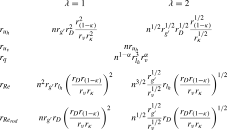
If we add the further constraint that the two processes have an equal Reynolds number of the current and an equal Reynolds number of the rods, that is  $r_{Re}=r_{Re_{rod}}=1$, results in $r_D=nr_{l_{h}}$ and $r_{u_{h}}=r_{\nu }/(nr_{l_{h}})$ and yields
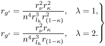 \begin{equation}
\left. \begin{array}{@{}ll@{}}
r_{g'}=\dfrac{r_{\nu}^2r_{\kappa}^2}{n^4r_{l_{h}}^3r_{(1-\kappa)}^{2}},
& \lambda=1,\\
r_{g'}=\dfrac{r_{\nu}^2r_{\kappa}}{n^4r_{l_{h}}^3r_{(1-\kappa)}},
& \lambda=2. \end{array}\right\}
\end{equation}
\begin{equation}
\left. \begin{array}{@{}ll@{}}
r_{g'}=\dfrac{r_{\nu}^2r_{\kappa}^2}{n^4r_{l_{h}}^3r_{(1-\kappa)}^{2}},
& \lambda=1,\\
r_{g'}=\dfrac{r_{\nu}^2r_{\kappa}}{n^4r_{l_{h}}^3r_{(1-\kappa)}},
& \lambda=2. \end{array}\right\}
\end{equation}
Table 6 lists the similarity ratios computed for  $\lambda =1,2$ by imposing the same values of $Re$ in the two processes and the same $Re_{rod}$ in the two processes; there are five degrees of freedom in selecting the scale ratios. In practical case, these similarity rules are too restrictive and essentially not necessary as long as, for instance, we have $Re$ and $Re_{rod}$ in the two processes to guarantee the same $\lambda$ in the two processes.
Table 6. Similarity ratios computed by imposing  $r_{Re}=1$ and $r_{Re_{rod}}=1$ for the two cases $\lambda =1$ and $\lambda =2$, distorted model.

We note that large variations of  $r_{\kappa }$ are accompanied by small variations of $r_{(1-\kappa )}$ hence this last scale ratio can be assumed constant.
If we wish to extrapolate, e.g. exp. 11 in our tank (model) to a prototype scale (real field), assuming  $r_{l_{h}}=1/20$, $n=5$, $r_{\kappa }=r_{(1-\kappa )}=1$, $r_{\nu }\approx 1$, $r_D=4$ and $r_{g'}=1/2$ and $\lambda =2$, results in $r_{u_{h}}=3.16$, $r_{u_{v}}=15.8$, $r_{Re}=0.79$, $r_{Re_{rod}}=12.6$. We refer to the rules listed in table 5. The current is almost three times slower in the prototype than in the model, with $Re$ larger in the prototype than in the model but with the $Re_{rod}$ almost one tenth in the model than in the prototype. This last effect must be carefully checked in order to guarantee a sufficiently high value of $Re_{rod}$ also in the prototype. The inflow rate in the prototype is almost 25 times the inflow rate in the model. In dimensional variables, exp. 11 can be extrapolated to a real field GC of density $\rho _{c_{p}}\approx 1043\ \textrm {kg}\ \textrm {m}^{-3}$ advancing in water, released in the presence of vegetation with diameter $D_p=0.4\ \textrm {cm}$ and with an inflow rate (referred to the full circle) $q'_p\approx 61\ \textrm {l}\ \textrm {s}^{-1}$. The experimental initial front speed was $u_{N_{m}}=2.7\ \textrm {cm}\ \textrm {s}^{-1}$ in the model, resulting in $u_{N_{p}}\approx 0.85\ \textrm {cm}\ \textrm {s}^{-1}$ in the real field.
In practical situations, it may be necessary to reproduce a natural GC in the laboratory, to investigate certain aspects that may have escaped observation in the field, or to reconstruct measurements never made in the field, or to verify the consequences of accidents with environmental damages and possible pollution consequences. In these cases it is convenient to adopt the following rules.
(i) Reduce the horizontal geometric scale, with $r_{l_{h}}\ll 1$ in order to contain the model in the space available in the laboratory.
(ii) Choose a vertical scale greater than the horizontal one,
$n>1$, in order to generate, in the laboratory, currents with a thickness that can be measured with adequate accuracy: $n<10$ is also suggested to avoid an excessive distortion of the flow field.(iii) In order to reproduce the vegetation, select cylinders with an adequate diameter for the practical operations of laying, with
$r_D>1$.(iv) Maintain a ratio
$r_{g'}={O}(1)$ or slightly different, to facilitate the preparation of the fluid of the stream, using water as the ambient fluid.(v) Check that the required flow rate, with the chosen scale ratios, can be achieved with the pumps or the hydraulic circuit available in the laboratory.
(vi) The selection of
$r_{\kappa }, r_{(1-\kappa )}$ can be adapted to the needs, although it is advisable to have $r_{\kappa }={O}(1), r_{(1-\kappa )}={O}(1)$.(vii) Check that
$Re$ and $Re_{rod}$ are comparable in model and prototype. It may be convenient to increase the viscosity of the current fluid used in the experiments (e.g. by adding glycerol), with $r_{\nu }>1$, to modulate the Reynolds number values.


