


Explosive dispersal of granular media, whereby the detonation of a central explosive or sudden release of pressurized gases disperses densely packed particles to form dilute particle clouds, occurs in a wide range of natural phenomena and engineering processes (Formenti, Druitt & Kelfoun Reference Formenti, Druitt and Kelfoun2003; Eckhoff Reference Eckhoff2009; Aglitskiy et al. Reference Aglitskiy, Velikovich, Karasik, Metzler and Obenschain2010; Kuranz et al. Reference Kuranz2018; Frost Reference Frost2018). In volcanic eruptions, the explosive expansion of pressurized gases through an initially concentrated dispersion of particles expels mixtures of pressurized gases and fragments of magma within volcanic conduits (Marjanovic et al. Reference Marjanovic, Hackl, Shringarpure, Annamalai and Balachandar2018). For various commercial and military explosive systems, such as fire extinguishing devices using explosive dispersed dry powders (Klemens, Gieras & Kaluzny Reference Klemens, Gieras and Kaluzny2007), thermobaric and fuel-air bombs (Frost, Goroshin & Zhang Reference Frost, Goroshin and Zhang2010; Frost et al. Reference Frost, Grégoire, Petel, Goroshin and Zhang2012), the explosive dispersal of granular media and the ensuing mixing of particulate matter with air are of particular importance to their reliable applications (Zhang et al. Reference Zhang, Ripley, Yoshinaka, Findlay, Anderson and Rosen2015; Bai et al. Reference Bai, Wang, Xue and Wang2018; Posey et al. Reference Posey, Roque, Guhathakurta and Houim2021). Another prominent application involves blast mitigation by surrounding the explosive with a layer of particles (Milne et al. Reference Milne, Floyd, Longbottom and Taylor2014; Pontalier et al. Reference Pontalier, Loiseau, Goroshin and Frost2018). The transfer of heat and energy from explosives to the particles during shock compaction and the ensuing gas–particle interaction significantly reduce the blast overpressure and impulse.
Considerable effort has been devoted to understanding the explosive dispersal process of granular media, which involves complex multiphase coupling and spans a range of scales (Frost et al. Reference Frost, Goroshin and Zhang2010; Rodriguez et al. Reference Rodriguez, Saurel, Jourdan and Houas2013, Reference Rodriguez, Saurel, Jourdan and Houas2014; Xue, Sun & Bai Reference Xue, Sun and Bai2016; Osnes, Vartdal & Reif Reference Osnes, Vartdal and Reif2017; Frost Reference Frost2018; Kun et al. Reference Kun, Kaiyuan, Xiaoliang, Yixiang and Chunhua2018; Xue et al. Reference Xue, Cui, Du, Shi, Gan and Bai2018; Carmouze et al. Reference Carmouze, Saurel, Chiapolino and Lapebie2019; Chiapolino & Saurel Reference Chiapolino and Saurel2019; Fernandez-Godino et al. Reference Fernandez-Godino, Ouellet, Haftka and Balachandar2019; Mo et al. Reference Mo, Lien, Zhang and Cronin2019; Koneru et al. Reference Koneru, Rollin, Durant, Ouellet and Balachandar2020). In particular, most studies focus on the hierarchical jet-like structures observed in cylindrical and spherical geometries (Frost et al. Reference Frost, Goroshin and Zhang2010; Rodriguez et al. Reference Rodriguez, Saurel, Jourdan and Houas2013, Reference Rodriguez, Saurel, Jourdan and Houas2014; Xue et al. Reference Xue, Sun and Bai2016; Osnes et al. Reference Osnes, Vartdal and Reif2017; Frost Reference Frost2018; Kun et al. Reference Kun, Kaiyuan, Xiaoliang, Yixiang and Chunhua2018; Xue et al. Reference Xue, Cui, Du, Shi, Gan and Bai2018; Carmouze et al. Reference Carmouze, Saurel, Chiapolino and Lapebie2019; Chiapolino & Saurel Reference Chiapolino and Saurel2019; Fernandez-Godino et al. Reference Fernandez-Godino, Ouellet, Haftka and Balachandar2019; Mo et al. Reference Mo, Lien, Zhang and Cronin2019; Koneru et al. Reference Koneru, Rollin, Durant, Ouellet and Balachandar2020). The origin and evolution of particle jetting have been extensively investigated and found to be closely associated with the spatial distribution of disseminated particles and the terminal velocities (Kandan et al. Reference Kandan, Khaderi, Wadley and Deshpande2017; Loiseau et al. Reference Loiseau, Pontalier, Milne, Goroshin and Frost2018; Pontalier et al. Reference Pontalier, Loiseau, Goroshin and Frost2018; Li et al. Reference Li, Xue, Zeng, Tian and Guo2022), two prominent attributes relevant to pertinent applications. However, some fundamental questions that are of much interest to engineering applications remain left unaddressed. Specifically, how fast is dispersal completed? Are the dispersed particles homogeneously distributed in space? Is any nontrivial proportion of particles not expelled successfully? These three questions are critical to assessing three fundamental attributes of explosive dispersal, namely, efficiency, homogeneity and completeness. Since the explosive dispersal processes for systems with vastly varying scales and structural parameters may occur on markedly different time and length scales, adequately quantifying the key attributes is quite challenging, let alone properly characterizing distinctly different explosive dispersal processes. Here, by identifying and understanding the most significant events contributing to each respective attribute, we construct three dimensionless parameters to categorize various dispersal processes into distinct dispersal modes.
The complex particle-flow interaction plays an important role in the explosive dispersal of particles, especially the formation of particle jetting (Xu et al. Reference Xu, Lien, Ji and Zhang2013; Osnes et al. Reference Osnes, Vartdal and Reif2017; Carmouze et al. Reference Carmouze, Saurel, Chiapolino and Lapebie2019; Chiapolino & Saurel Reference Chiapolino and Saurel2019; Fernandez-Godino et al. Reference Fernandez-Godino, Ouellet, Haftka and Balachandar2019; Mo et al. Reference Mo, Lien, Zhang and Cronin2019; Koneru et al. Reference Koneru, Rollin, Durant, Ouellet and Balachandar2020; Li et al. Reference Li, Xue, Zeng, Tian and Guo2022). Based on particle resolved numerical investigations, Xu et al. (Reference Xu, Lien, Ji and Zhang2013) and Mo et al. (Reference Mo, Lien, Zhang and Cronin2019) observed that the microgas jets that formed at the internal surface of the particle ring penetrated the particle layer through gaps created by the inelastic collision between particles, generating high-speed particle agglomerates. Recently, shock-driven multiphase instability (SDMI), a variant of the classic Richtmyer–Meshkov (RM) instability, was reported to be responsible for particle jetting in dilute systems (Osnes et al. Reference Osnes, Vartdal and Reif2017; Chiapolino & Saurel Reference Chiapolino and Saurel2019; Koneru et al. Reference Koneru, Rollin, Durant, Ouellet and Balachandar2020). In contrast, another interfacial instability, shock-driven granular instability (SDGI), is proposed to account for the jetting of shock-loaded dense granular interfaces (Li et al. Reference Li, Xue, Zeng, Tian and Guo2022). Although these particle-flow interaction mechanisms provide important insights into the physics underlying particle dispersal, they fail to incorporate the coupling between the expanding ring as an entirety and the evolving central pressure field, which governs the dynamics of the particle ring. One striking phenomenon resulting from macroscale particle-flow coupling is the pulsation of the particle ring analogous to the pulsation of the gas bubble generated in the underwater explosion (Wang et al. Reference Wang, Gui, Zhang, Gao, Xu and Jia2021). The pulsation of the particle ring sustained by the central explosion, albeit rarely reported, is essential to understand the overall dispersal behaviour of the particle ring. The emergence, prevalence and waning of the particle ring pulsation must be understood based on the varying particle-flow coupling regimes, which can be quantified by calculating the characteristic time scale ratios of signature events.
As highlighted in many investigations involving shock/blast-driven particle-laden compressible flows, understanding or even predicting the behaviour of these flows requires knowledge of particle-scale phenomena, such as particle‒particle collisions, particularly in dense particle flows, shock-particle interactions and the coupling between particle and flow jetting (Osnes et al. Reference Osnes, Vartdal and Reif2017; Sundaresan, Ozel & Kolehmainen Reference Sundaresan, Ozel and Kolehmainen2018; Carmouze et al. Reference Carmouze, Saurel, Chiapolino and Lapebie2019; Chiapolino & Saurel Reference Chiapolino and Saurel2019; Mo et al. Reference Mo, Lien, Zhang and Cronin2019; Koneru et al. Reference Koneru, Rollin, Durant, Ouellet and Balachandar2020; Tian et al. Reference Tian, Zeng, Meng, Chen and Xue2020). Thus, we conducted four-way coupled two-dimensional (2-D) Euler‒Lagrange simulations of the explosive dispersal of the particle ring wherein the denotation of the cylindrical burster was simulated by the sudden release of pressurized gases in the central gas pocket. A numerical protocol was established that allowed us to convert the dispersal process driven by the central detonation to the equivalent process driven by the pressurized gases and vice versa. Using this protocol, we performed a range of simulations for dispersal systems with varying structures, including the energy of pressurized gases, the mass of the particle ring, and the packing fraction of particles. Regardless, systems with the same mass ratio of particles to central gases, M/C = mring/mgas, display similar dispersal behaviours, highlighting the role of M/C as one primary governing parameter. We developed theoretical models based on the continuum assumption to account for the shock compaction phase and the ensuing pulsation of the particle ring and to predict the dispersal mode for a particular dispersal system. The combined models are capable of identifying the ideal dispersal mode while falling short of recognizing the other three modes, which require knowledge of grain-scale particle loosening mechanisms.
The paper is organized as described below. In § 1, the numerical method is presented, followed by the description of the numerical setup in § 2. A variety of macroscale behaviours of dispersed particle rings are elaborated in § 3, which are characterized using three prominent attributes and categorized into different modes. The macroscale particle-flow coupling and its correlation with the dispersal mode are explored in § 4. The dominant mesoscale dispersal structures are discussed in § 5. Finally, the results are summarized in § 6.
1. Numerical method
Numerical simulations were performed based on coarse-grained compressible computational fluid dynamics–discrete parcel method (CCFD-DPM), a coarse-grained Euler–Lagrange numerical approach suitable for gas–particle flows in laboratory-scale systems (Sundaresan et al. Reference Sundaresan, Ozel and Kolehmainen2018; Tian et al. Reference Tian, Zeng, Meng, Chen and Xue2020). The CCFD-DPM approach tracks and accounts for parcel–parcel contact interactions. Each parcel consists of multiple physical particles with the same physical and kinetic properties. The number of real particles that represent a computational parcel is quantified using a scaling factor called the super particle loading, χ, whose value is set based on the volume/mass fraction of the particles and computational memory available. For particle-gas systems, the value of χ reported in the previous literature ranges from O(101) to O(103) (Osnes et al. Reference Osnes, Vartdal and Reif2017; Koneru et al. Reference Koneru, Rollin, Durant, Ouellet and Balachandar2020). In the present study, χ is of the order of O(101).
For the gas phase, the volume-averaged governing equations ((1.1)–(1.3)) constructed in the Eulerian frame are based on a five-equation transport model, i.e. a simplified form of the Baer–Nunziato (B-N) model, which has been modified to account for compressible multiphase flows ranging from dilute to dense gas–particle flows (Baer & Nunziato Reference Baer and Nunziato1986):
 \begin{gather}\frac{{\partial ({\phi _f}\langle {\rho _f}\rangle )}}{{\partial t}} + \boldsymbol{\nabla }\boldsymbol{\cdot }({\phi _f}\langle {\rho _f}\rangle {\boldsymbol{\tilde{u}}_f}) = 0,\end{gather}
 \begin{gather}\begin{array}{ccccc} \dfrac{{\partial ({\phi _f}{{\boldsymbol{\tilde{u}}}_f}\langle {\rho _f}\rangle )}}{{\partial t}} + \boldsymbol{\nabla }\boldsymbol{\cdot }({\phi _f}\langle {\rho _f}\rangle {{\boldsymbol{\tilde{u}}}_f}{{\boldsymbol{\tilde{u}}}_f} + {\phi _f}\langle {P_f}\rangle )\\ = \langle {P_f}\rangle \boldsymbol{\nabla }{\phi _f} + \sum\limits_i {\{ {\phi _{p,i}}{\rho _{p,i}}{D_{p,i}}({{\boldsymbol{\tilde{u}}}_{p,i}} - {{({{\boldsymbol{\tilde{u}}}_f})}_i})\} } , \end{array}\end{gather}
 \begin{gather}\begin{array}{ccccc} \dfrac{{\partial ({\phi _f}\langle {\rho _f}\rangle {{\tilde{E}}_f})}}{{\partial t}} + \boldsymbol{\nabla }\boldsymbol{\cdot }({\phi _f}\langle {P_f}\rangle {{\tilde{E}}_f}{{\boldsymbol{\tilde{u}}}_f} + {\phi _f}\langle {\rho _f}\rangle {{\boldsymbol{\tilde{u}}}_f})\\ = \langle {P_f}\rangle \boldsymbol{\nabla }{\phi _f} \boldsymbol{\cdot} {{\boldsymbol{\tilde{u}}}_p} + \sum\limits_i {\{ {\phi _{p,i}}{\rho _{p,i}}{D_{p,i}}({\boldsymbol{u}_{p,i}} - {{({{\boldsymbol{\tilde{u}}}_f})}_i}) \boldsymbol{\cdot} {{\boldsymbol{\tilde{u}}}_{p,i}}\} } . \end{array}\end{gather}
 The gas volume fraction, velocity, density, pressure and total energy of the gas are represented by ϕf, uf, ρf, Pf and Ef, respectively, where Ef = ρfef + 0.5 uf uf. In (1.1)–(1.3),  $\left\langle {} \right\rangle $ and $\widetilde {}$ denote phase-averaged and mass-averaged variables, respectively, ρp.i and up,i represent the density and velocity of parcel i, respectively, Dp,i is the drag force coefficient of parcel i and ϕp.i = wi,fVp,i/Vf is the contribution of parcel i to the weighted particle volume fraction (wi,f is the distributed weight that parcel i contributes to the particle volume fraction in fluid cell f, and Vp,i and Vf are the volumes of parcel i and the fluid cell, respectively).
We employ the Di Felice model combined with Ergun's equation ((1.4)–(1.7)) to calculate Dp (Felice Reference Felice1994), which considers the effects of both the particle Reynold number, Rep, and the particle phase volume fraction, ϕp, and has been widely used in particle-laden multiphase flows:
 \begin{gather}{D_{p,i}} = \frac{3}{{8{\rho _p}/{\rho _f}}}{C_d}\frac{{|{\boldsymbol{u}_f} - {\boldsymbol{u}_{p,i}}|}}{{{r_p}}},\end{gather}
 \begin{gather}{C_d} = \frac{{24}}{{R{e_p}}}\left\{ {\begin{array}{@{}ll} {8.33\dfrac{{{\phi_p}}}{{{\phi_f}}} + 0.0972R{e_p}}&{\textrm{if}\;{\phi_f} < 0.8}\\ {{f_{base}} \phi_f^{ - \zeta }}&{\textrm{if}\;{\phi_f} \ge 0.8} \end{array}} \right.,\end{gather}
 \begin{gather}{f_{base}} = \left\{ {\begin{array}{@{}ll} {1 + 0.167Re_p^{0.687}}&{\textrm{if}\;R{e_p} < 1000}\\ {0.0183R{e_p}}&{\textrm{if}\;R{e_p} \ge 1000} \end{array}} \right.,\end{gather}
 \begin{gather}\zeta = 3.7 - 0.65\exp [ - {\textstyle{1 \over 2}}{(1.5 - {\log _{10}}R{e_p})^2}].\end{gather}
In (1.4) and (1.5), Cd is the dimensionless coefficient of the drag force and rp is the particle radius. For dense particle flows (ϕf < 0.8), (1.4) reduces to the original Ergun equation. Otherwise, Cd takes the form of Stokes's law multiplied by a factor of fbase, which varies with Rep, as indicated by (1.6) and (1.7).
The particle phase is represented by discrete parcels whose motion is governed by Newton's second law ((1.8) and (1.9)):
 \begin{gather}\frac{{\textrm{d}{\boldsymbol{u}_{p,i}}}}{{\textrm{d}t}} = {D_{p,i}}({\boldsymbol{u}_f} - {\boldsymbol{u}_{p,i}}) - \frac{1}{{{\rho _p}}}\boldsymbol{\nabla }\langle {P_f}\rangle + \frac{1}{{{m_p}}}\sum\limits_j {{\boldsymbol{F}_{C,ij}}} ,\end{gather}
 \begin{gather}\frac{{\textrm{d}\kern0.7pt{\boldsymbol{x}_{p,i}}}}{{\textrm{d}t}} = {\boldsymbol{u}_{p,i}},\end{gather}
where up,i and xp,i denote the velocity and displacement of parcel i, respectively, and FC,ij represents the collision force between parcels i and j.
A four-way coupling strategy was adopted to account for the momentum and energy transfer between gases and particles. Specifically, the particle drag force and the associated work were incorporated into the momentum and energy equations of the gas phase as the source terms. The particle parcels are driven by the pressure gradient force, drag force and collision force between parcels (1.8). A soft sphere model, which is represented by a linear-spring dashpot model, was employed to model the collision force between parcels. Hence, FC,ij consists of a repulsive force and a damping force:
 \begin{equation}{\boldsymbol{F}_{C,ij}} = {k_{n,p}}{\boldsymbol{\delta}_n} - {\gamma _{n,p}}{\boldsymbol{u}_{n,ij}},\end{equation}
where kn,p and γn,p are the stiffness and damping coefficients of parcels, respectively, and δn and un,ij are the overlap and difference in the normal velocity between parcels in contact, respectively. Here, γn,p is a function of the parcel restitution coefficient εp:
 \begin{equation}{\gamma _{n,p}} ={-} \frac{{2\ln {\varepsilon _p}}}{{\sqrt {{{\rm \pi}^2} + \ln {\varepsilon _p}} }}\sqrt {{m_p}{k_{n,p}}} .\end{equation}
The weighted essentially non-oscillatory (WENO) scheme was used to reconstruct the primary flow variables and solve the equations governing the gases. A Riemann solver proposed by Harten, Lax and van Leer was used to obtain the intercell fluxes. The third-order Runge–Kutta method was applied for time integration. The equations describing the parcel velocity and position were discretized using the velocity-Verlet algorithm. Bilinear/trilinear interpolation functions were adopted to calculate the particle volume fraction and source terms on the Eulerian grids, as well as the fluid variables on Lagrangian parcels (Liu, Osher & Chan Reference Liu, Osher and Chan1994). Numerical details of CCFD-DPM are available in our previous publication (Tian et al. Reference Tian, Zeng, Meng, Chen and Xue2020). The CCFD-DPM framework introduced the variable A and has been validated in several benchmark experiments involving shock-driven particle-laden flows (Tian et al. Reference Tian, Zeng, Meng, Chen and Xue2020), such as experiments performed by Rogue et al. (Reference Rogue, Rodriguez, Haas and Saurel1998), which investigate shock dissipation through particle curtains; the experiments conducted by Britan & Ben-Dor (Reference Britan and Ben-Dor2006), which assess both the gaseous and solid pressures inside particle columns impinged head on by shocks; and the experiments assessing shock-induced interfacial instability of granular media (Kun et al. Reference Kun, Kaiyuan, Xiaoliang, Yixiang and Chunhua2018).
Notably, for dispersal systems where a central burster is enclosed by ductile or brittle particles, the deformation and/or fracture of particles and the sintering between particles are inevitable for particles adjacent to the burster. These phenomena may well affect the ensuing dispersal, particularly for systems with thin particle shells. Since the current CCFD-DPM framework does not account for these particle-scale phenomena, we must be aware of the scenario in which the simulations and the related discussions are valid, namely, either the explosive sources are so mild that the particle-scale phenomena are negligible, or particles are composed of materials with a combination of high compressive strength, high toughness and moderate/high hardness. Otherwise, the particle-scale phenomenon may cause the actual dispersal to deviate from that predicted by the framework in which these particle-scale phenomena are excluded.
2. Numerical set-up
The two-dimensional (2-D) configuration shown in figure 1(a) serves as an archetypical system to investigate the explosive dispersal behaviour of particle rings. Instead of the burster used in the explosive dispersal experiment, the numerical simulations employ a high-pressure gas pocket with a radius of Rgas ,0 filled with air to disperse the enclosing ring consisting of 2-D disks with varying packing fractions, ϕ 0. For the investigated dispersal systems described below, the initial radius and temperature of the gas pocket remain constant, Rgas ,0 = 20 mm and T 0 = Tamb = 298 K, respectively, while the initial pressure P 0 varies. The radius expansion algorithm is used to generate the particle packing with a given ϕ 0 in an annular domain with the inner and outer radii of Rin ,0 and Rout ,0, respectively. A population of disk-like parcels with artificially small radii ensure no parcel overlap is randomly created within the specified domain. Then, all parcels are expanded until the specified parcel size distribution and desired packing fraction are both satisfied. The real 2-D particle has a diameter of 100 μm, while the diameter of the parcel uniformly ranges from 360 to 780 μm to avoid potential crystallization during shock compaction. Due to the use of computational parcels, the collision distance must be modified in the same manner as the parcel diameter. A random but homogenous arrangement of parcels is achieved, as shown in the zoomed-in inset of figure 1(a), where the parcels are coloured according to the local Voronoi packing fraction, ϕp,voro. The parcel has a density of 2500 kg m−3, which is the same as the real particles. The restitution coefficient, εp, is set to 0.6, which accounts for the energy dissipation inside the parcel; the normal stiffness of contacts between parcels is set to 2 × 10⁷ N m−1.

Figure 1. (a) A quarter of the two-dimensional numerical configuration wherein the central gas pocket is enclosed by a particle ring consisting of polydispersed computational parcels. Inset shows the zoomed-in arrangement of particle packing. (b) Distribution of the structural parameters, P 0, h, ϕ 0 as well as the resulting M/C for dispersal systems which are to be numerically investigated. Here, h is the ring thickness, h = Rout ,0 – Rin ,0.
Evidently, a host of structural variables characterize the dispersal system and play a role in the resulting dispersal behaviour with varying levels of relative importance. Instead of performing a conventional parametric study, we focus on their combined effects manifested by one single dimensionless parameter, the mass ratio, M/C, which defines the energy imparted to the confining materials per unit mass. Previous studies have accentuated the fundamental role played by the M/C in explosive dispersal by correlating the initial expansion velocity of disseminated particles with the M/C (Loiseau et al. Reference Loiseau, Pontalier, Milne, Goroshin and Frost2018; Pontalier et al. Reference Pontalier, Loiseau, Goroshin and Frost2018). The structural variables denoted in figure 1(a) all contribute to the mass ratio M/C, as expressed in (2.1):
 \begin{equation}M/C = \frac{{{\rm \pi}(R_{out,0}^2 - R_{in,0}^2){\phi _0}{\rho _p}}}{{{\rm \pi} R_{gas}^2{\rho _{gas}}}} = \frac{{(R_{out,0}^2 - R_{in,0}^2){\phi _0}{\rho _p}R{T_0}}}{{R_{gas}^2{P_0}}},\end{equation}
where R is the specific gas constant of air,  $R=288.7\ {\rm J}/{\rm kg}/{\rm K}$. The mass ratio clearly does not reflect the nature of various explosive sources with vastly different specific energies. Hence, two dispersal systems with the same M/C but different explosive sources, for instance, the burster and the pressurized gas pocket, will undoubtedly exhibit distinct dispersal behaviours. In Appendix A, we propose a mass ratio conversion between systems with different explosive sources based on the energy equivalent principle whereby the dispersal behaviours exhibited by the systems with explosive sources other than pressurized gases are incorporated into the dispersal mode classification framework proposed in § 3.3.
As illustrated in figure 1(b), by varying the values of P 0, Rout ,0 and ϕ 0, the mass ratio M/C for the simulated dispersal systems ranges from 9.7 to 6800, as marked in figure 1(b), spanning four orders of magnitude. Three different values of ϕ 0, namely, 0.5, 0.6 and 0.65, were used to represent loose, dense and densest random packings, respectively. Notably, the packing fraction values presented throughout this work are those of the equivalent three-dimensional (3-D) packings derived from the conversion between the packing fractions in the 2-D and 3-D packings proposed by Borchardt-Ott (Reference Borchardt-Ott2012):
 \begin{equation}{\phi _{3\text{-D}}} = 0.2595 + \frac{{{\phi _{2\text{-D}}} - 0.0931}}{{0.2146 - 0.0931}}(0.4760 - 0.2595).\end{equation}
Hence, the 3-D particle packing fractions ϕ 3D = 0.5, 0.6 and 0.65 correspond to the 2-D particle packing fractions ϕ 2D = 0.77, 0.83 and 0.86, respectively. For each M/C, at least three systems with different combinations of P 0, Rout ,0 and ϕ 0 were constructed to assess the variability of the results. In total, we performed explosive dispersal simulations for 70 different systems with 20 different values of M/C. For clarity, the system is labelled with four symbols, M/C, P 0 (in units of bar), the thickness of the ring ( $h = {R_{out,0}} - {R_{in,0}}$, in units of mm) and ϕ 0.
3. Results
3.1. Macroscale dispersal behaviour
A space–time (R–t) diagram showing the spaciotemporal variations in the particle packing fraction ϕp(R, t) was constructed using the circumferentially averaged ϕp to understand the overall explosive dispersal behaviour of the particle ring. Figure 2(a–d) displays four typical R–t diagrams for systems with different M/C values. Upon the release of pressurized gases, an incident shock wave impinges on the inner surface of the particle ring (the dynamics of shocks are illustrated in figure 3a), resulting in a compaction front (CF) traversing the particle bed. Across the CF, ϕ 0 immediately jumps to ϕcomp, the packing fraction of the compacted particles. A rarefaction wave (RW) reflects off the external surface of the particle ring upon the arrival of the CF, resulting in a discernible decrease in ϕp in its wake. The dynamics of CF and the ensuing RW are sufficiently recognized in the R–t diagram of the volumetric strain rate  ${\dot{\varepsilon }_v}$ in particles (the calculation of ${\dot{\varepsilon }_v}$ is presented in Appendix B), as plotted in figure 2(e).

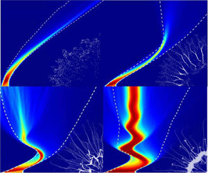
Figure 2. R–t diagrams of the ϕp of particle rings in the dispersal system (a) 9.7-245-10-0.5, (b) 103.7-100-30-0.6, (c) 1024-20-50-0.6 and (d) 4875-20-140-0.6. (e) R–t diagrams of the volumetric strain rate  ${\dot{\varepsilon }_v}$ in particles in the dispersal system 494-200-140-0.6. CF, compaction front; RW, rarefaction wave. The white and pink dashed lines indicate the boundaries delimiting the particle cloud, IPF and OPF, and dense core band (CB), ISCB and OSCB, respectively.

Figure 3. (a) Temporal variations in ϕp,ave for typical dispersal systems. (b) Scaled temporal variations in ϕp,ave for the same systems shown in panel (a) wherein the time is scaled by tring.
Despite similar early-time shock compaction phases, systems with different M/C ratios proceed with distinctly different late-time dispersal phases. The ring in system 9.7-245-10-0.5 undergoes persistent expansion, while particle shedding progressively disintegrates the ring from inwards to outwards (figure 2a). In contrast, as shown in figure 2(b), the ring in system 103.7-100-30-0.6 remains densely packed during expansion, which strikingly proceeds to undergo noticeable contraction accompanied by significant outbound particle jetting commencing from the outer surface (see the inset in figure 2b). The contraction observed in system 103.7-100-30-0.6 becomes more pronounced in system 1024-20-50-0.6, wherein a densely packed core band (CB) not only survives the entire contraction but also embarks on a second expansion (figure 2c). The internal and external surfaces of the densely packed CB, ISCB and ESCB are defined such that the packing fraction of bulk enclosed by ISCB and ESCB remains above 0.3. Only 5 % of the volume of particles resides inside the inner particle front (IPF) and another 5 % resides beyond the outer particle front (OPF). The trajectories of the IPF, OPF, ISCB and OSCB are superimposed in figures 2(c) and 2(d).
At the onset of the second expansion of the CB, inbound particle jetting initiated from the ISCB occurs (figures 2c and 2d). In contrast to the internal particle shedding during the first ring expansion, as observed in system 9.7-245-10-0.5 (figure 2a), where the loose particles still move outwards, the particles entrained by the inbound particle jets travel inwards, eventually moving to the central area. The relatively short-lived CB in system 1024-20-50-0.6 becomes enduring in system 4875-20-140-0.6 and we observe multiple pulsations of CB with decreasing amplitudes (see figure 2d). Notably, inbound and outbound particle jetting occur at each contraction-to-expansion and expansion-to-contraction turning point, respectively. Particle shedding, and inbound and outwards particle jetting are elaborated in § 5.
3.2. Characterization of dispersal behaviour
The diverse dispersal behaviours of particles shown in figures 2(a)–2(d) lead to a fundamental question: Can we properly characterize and classify the diverse dispersal processes? This question is critical for adequately evaluating the dispersal process and tailoring the dispersal systems for a specific application. In this section, we aim to address this question by establishing a unified characterization framework.
Unarguably, efficiency is among the most important properties of the dispersal process from an engineering perspective. The time required for the packed particles to be dispersed into a dilute state, tdis, is a useful indicator of the dispersal efficiency, although tdis scales with the length scale of the system. Here, the dispersed ring is referred to as dilute when the average particle volume fraction in the annular region delimited by IPF and OPF, ϕp,ave, is less than 0.1. Figure 3(a) plots the variations in ϕp,ave in several typical dispersal systems. Notably, one or more kinks are commonly observed in ϕp,ave(t) curves, which are caused by the sudden deflections of IPF or OPF due to the burst of inbound or outbound particle jetting. As expected, systems with an increased M/C, due to heavier particle rings, smaller input energies or both, take more time to be dispersed to the nominal dilute state. As indicated in figure 4(a), tdis increases logarithmically with the M/C and approaches infinity when the M/C is greater than 2000. For systems with an M/C of O(103), ϕp,ave does not reach 0.1 during the computational time. Hence, tdis was determined by extrapolating the ϕp,ave(t) curves, as described in Appendix C.

Figure 4. Variations in (a) tdis, (b) tring, (c) tdense with M/C. The dashed portions of tdis(M/C) and tdense(M/C) curves at the upper limit of the M/C range suggest tdis and tdense herein approach infinity rather than have definite values.
We instead use a dimensionless parameter ξ as the efficiency indicator by scaling tdis with the characteristic time of the ring expansion, tring, ξ = tdis/tring, to properly evaluate the efficiency of dispersal processes in systems with varying M/C values. Here, tring is the time it takes the ring to expand to twice the initial diameter, namely, tring = Rout ,0/Vout, with Vout representing the initial surface expansion velocity of the ring. The M/C dependence of tring is plotted in figure 4(b). Figure 3(b) depicts the variations in ϕp,ave with scaled time t/tring, with significantly reduced deviations observed between ϕp,ave(t) curves for different systems. Figure 5 shows the variation in ξ with M/C, and the error bars represent the variability between systems with different combinations of P 0, Rout ,0 and ϕ 0. For values less than a threshold mass ratio (M/C)ξ ~ 2500, ξ randomly fluctuates below 10. Afterwards, ξ increases above 10 and approaches infinity towards the upper limit of the M/C range. Therefore, the dispersion is at least one order slower than the ring expansion. For efficient dispersal, the dispersion should be completed during the time scale of ring expansion, leading to the criterion for the efficiency:
 \begin{equation}\xi < 10.\end{equation}
Another issue that is equally important is the spatial concentration of the dispersed particles, which is strongly affected by the emergence of densely packed CB, as shown in figures 2(c) and 2(d). If the CB survives for the entire dispersal time, tdis, the bulk of particles will adhere inside the narrow CB, although the nominal dilute state has been achieved. This dispersal process, albeit efficient, is highly inhomogeneous. Figure 4(c) presents the variation in tdense with M/C, which is fitted by an exponential function asymptotically approaching infinity. Rings in the systems with an M/C ratio larger than 1600 undergo slowly decaying pulsation and eventually dwell in an annular region located not far from its initial position, leading to an infinite tdense. The derivation of tdense for the systems with the enduring CB is described in detail in Appendix C. The ratio between the CB survival duration to the dispersal time, which is defined as κ = tdense/tdis, produces a homogeneity indicator. The M/C dependence of κ plotted in figure 5 shows a similar trend with ξ(M/C). Here, κ remains below unity until M/C exceeds a threshold, (M/C)κ ~ 500, beyond which κ increases above unity, substantially increases with M/C and eventually approaches infinity at the upper limit of the M/C range. A homogeneous dispersal does not allow the presence of the CB at the end of the dispersal. Accordingly, the criterion for homogenous dispersal is expressed as follows:
 \begin{equation}\kappa < 1.\end{equation}
Figure 5. M/C dependences of dimensionless parameters ξ, κ and χ. The critical M/C values corresponding to the thresholds for the efficiency, homogeneity and completeness, (M/C)ξ, (M/C)κ and (M/C)χ are indicated.
In addition to efficiency and homogeneity, a third issue related to dispersal completeness becomes prominent, as a non-trivial proportion of particles is observed to dwell in the central area, as shown in figures 2(c) and 2(d). The incompleteness of dispersal is conspicuously the undesired outcome for most applications. Therefore, the extent of dispersal completeness should be regarded as one of the essential dispersal properties. The volume fraction of particles eventually residing inside the central region, χ, is a suitable measurement of the completeness. Estimating χ in systems where inbound particle jetting has not yet ceased during the computational times received special attention (a detailed description of the estimation method is provided in Appendix C). Figure 5 shows the variation in χ with M/C. The χ(M/C) curve exhibits a plateau below 0.1 as M/C increases from O(100) to O(102) until M/C reaches a threshold, (M/C)χ ~ 250. A substantial increase in χ(M/C) ensues, accompanied by strong fluctuations between 0.3 and 0.6. Complete dispersal is expected for a minimum fraction of particles residing in the central area at the end of dispersal. We thus set the criterion for complete dispersal as follows:
 \begin{equation}\chi < 0.1.\end{equation}
Notably, the M/C thresholds corresponding to the three criteria are in the sequence of (M/C)χ < (M/C)κ < (M/C)ξ. Specifically, (M/C)ξ is one order larger than (M/C)χ and M/C)κ.
3.3. Classification of the dispersal mode
With the aid of the criteria for the efficiency, homogeneity and completeness of explosive dispersal, diverse dispersal behaviours are classified into four distinct modes, namely: (i) an ideal dispersal that satisfies all three criteria for efficiency, homogeneity and completeness ((3.1)–(3.3)); (ii) partial dispersal that satisfies the criteria for efficiency and homogeneity but fails to meet the criterion for completeness; (iii) retarded dispersal that only meets the criterion for efficiency; and (iv) failed dispersal that meets none of the three criteria. The classification of various dispersal processes in the parameter space of ξ, κ and χ is illustrated in figure 6, where the symbols representing the dispersal systems are rendered according to the respective M/C value. As the M/C increases from O(100) to O(101), to O(102), and finally to O(103) and higher, the dispersal mode transitions from ideal to partial, retarded and finally to failed, highlighting the dominant role played by the M/C in determining the dispersal mode. In explosive dispersal experiments using bursters as explosion sources, the retarded and failed dispersal modes are rarely observed because the maximum (M/C)exp in the reported experiments rarely reaches the order of O(102) (Loiseau et al. Reference Loiseau, Pontalier, Milne, Goroshin and Frost2018; Pontalier et al. Reference Pontalier, Loiseau, Goroshin and Frost2018), which is equivalent to (M/C)gas (gases at ambient temperature) of the order of O(100) (see Appendix A) and most likely corresponds to the ideal or partial dispersal modes.

Figure 6. Mode categorization of various dispersal systems in the parameter space of ξ, κ and χ. Dispersal systems classified into different dispersal modes are denoted by symbols with distinct shapes. Symbols are coloured according to the M/C of the corresponding system.
We should be fully aware that the order of magnitude rather than the actual values of the M/C thresholds, (M/C)i (i = ξ, κ, χ), indicated in figure 5, serves as the preliminary guide for the design or evaluation of the dispersal system. The phase map constructed in the parameter space shown in figure 6 provides a more reliable and refined framework. However, the calculation of ξ, κ and χ for a specific dispersal system requires knowledge of the whole dispersal process, which is often inaccessible or only accessible in hindsight. Therefore, the correlation between the structure of the dispersal system and the resulting dispersal mode must be established, which requires an in-depth understanding of the physics governing the transitions between different dispersal modes.
4. Analysis
4.1. Macroscale particle-flow coupling
The dynamics of the particle ring driven by the central pressurized gases are primarily governed by the complex coupling between particles and central flows. Figures 7(a)–7(d) present the space–time (R–t) diagrams of the pressure fields for the systems shown in figures 2(a)–2(d), where the circumferentially averaged gas pressure is used to plot the R–t diagrams. Similar to the dispersal behaviour of particle rings, the central flow field undergoes a two-stage evolution. The first stage, coinciding with the shock compaction phase of the ring, is dominated by the reciprocation of shock fronts between the centre and the inner surface, as evident in figure 7(a). Each incident shock invokes a CF traversing the particles, which is discernible in figure 2(e). The reciprocation of shock fronts becomes invisible after the significant expansion of the inner surface of the ring. Thereafter, the rapid expansion of the ring induces the overexpansion of the central gases, leading to a substantial decrease in pressure and eventually the reversal of the pressure gradient direction. Subject to the inwards directed pressure gradient forces, the expanding ring decelerates and tends to implode, which subsequently promotes the recovery of the pressure in the central gas pocket. Once the central pressure is increased above the ambient pressure, the outwards directed pressure gradient forces are restored across the thickness of the ring. The pinching ring subsequently gains outwards momentum, with a second expansion likely ensuing. This macroscale particle–gas coupling is adequately manifested by the synchronization between the pulsation of the particle ring and the fluctuation of the pressure inside the gas pocket, as plotted in figure 8(a), which share the same frequency with a 1/2 phase difference.

Figure 7. R–t diagrams of circumferentially averaged pressure in the dispersal system (a) 9.7-245-10-0.5, (b) 103.7-100-30-0.6, (c) 1024-20-50-0.6 and (d) 4875-20-140-0.6. The white and pink dashed lines indicate the IFP (OPF) and ISCB (ESCB), respectively.

Figure 8. (a) Fluctuations of the centre of mass of CB in terms of RCB(t) and the pressure in the centre, Pg(R = 0). (b) Temporal variation in mass fraction of gases retained inside the gas pocket, χg, in the system 1024-20-50-0.6 and 4875-20-140-0.6. (c) Radial profiles of pressure across the thickness of ring at three sequent contraction-to-expansion transitions in the system 4875-20-140-0.6. The dotted lines in panels (a) and (b) indicate the overall temporal variations in the averaged RCB, peak Pg and peak χg.
The pulsation of the particle ring resembles the pulsation of a gas bubble in the scenario of an underwater explosion (Wang et al. Reference Wang, Gui, Zhang, Gao, Xu and Jia2021). In contrast to the enduring bubble pulsation in the underwater explosion, which slowly loses momentum mainly due to the weak viscous dissipation inside the water, the particle ring only sustains a limited number of pulsation cycles as a result of quickly weakening particle–gas coupling. Multiple causes should be considered. The inelastic collision and friction between particles modestly dissipate the kinetic energy of the ring, acting similar to the viscosity of fluids. Nevertheless, the net gas flow-out associated with the gas infiltration plays a major role in diminishing the particle–flow coupling. As indicated in figure 8(b), only 66 % and 38 % (mass fraction) of gases are retained in the gas pockets at the first expansion–contraction transitions in systems 4875-20-140-0.6 and 1024-20-50-0.6, respectively. Notably, the gases flow into the gas pocket when the central pressure becomes negative (i.e. below ambient pressure). Thus, the χgas fluctuates in sync with the central pressure but decreases in the long term, indicating net gas loss over time. Consequently, the overall central pressure decreases with increasing damping fluctuation. The pressure difference between the central gas pocket and the ambient gas outside the CB is accordingly quickly normalized, as indicated by the flattening of the radial profiles of pressure across the thickness of the ring, as shown in figure 8(c), substantially reducing the primary driving forces of particles, namely, the pressure gradient forces and drag forces.
Two other important mechanisms are responsible for dissolving the particle–flow coupling, as illustrated in figure 9. As shown in figure 9(a), the initial impulse imparted to the particle ring is sufficiently strong to enable the expanding ring to quickly break away from the influence of the central flows. Likewise, the central gas pocket barely experiences the presence of the ring. This scenario occurs in systems with an M/C of the order of O(100) (see figures 2a and 7a). However, the particle–gas coupling is sustained only if the ring, more precisely the densely packed CB, continues to provide sufficient confinement for the gas pocket. Once the CB disintegrates, the central gases thrust out, terminating particle–gas coupling (figure 9b).

Figure 9. Illustrations of two particle–flow decoupling mechanisms. (a) Fast expanding DB escapes the central flows with negative Pg. (b) DB prematurely disintegrates into the dilute particle cloud which cannot confine the central gases.
Different mechanisms dominate particle–gas coupling in different dispersal systems, leading to markedly varying degrees of particle–gas coupling. Here, we classify particle–gas coupling into decoupling, weak coupling, medium coupling and strong coupling regimes. In the decoupling regime, rings are only subjected to the initial impetus imparted by the central pressurized gases and thereafter evolve on their own (see figures 2a and 7a), which normally occurs in systems with an M/C of the order of O(100). In the weak coupling regime, the innermost layers of particles accumulate in the centre due to the negative overpressure (below the ambient pressure) inside the gas pocket, while the bulk of particles are dispersed into the outer space. This phenomenon is illustrated in figures 2(b) and 7(b). As more particles are influenced by the central negative pressure and accumulate in the centre, the particle–gas coupling is classified as medium. In the medium coupling regime, the contraction of the particle ring is a solitary event since the densely packed CB disintegrates during ring contraction, as shown in figures 2(c) and 7(c), which often leads to abnormally high proportions of undispersed particles. In contrast, the strong particle–gas coupling results in the persistent pulsation of the ring, more strictly speaking, the densely packed CB, as shown in figures 2(d) and 7(d).
Obviously, in the decoupling and weak particle–gas coupling regimes, only the minimum fraction of particles accumulates in the centre. However, in the medium and strong particle–gas coupling regimes, a non-trivial proportion of particles is hurled into the centre during each contraction-to-expansion transition. The dispersal accordingly becomes incomplete. The most disastrous scenario occurs when the ring disintegrates during the contraction, and hence, the majority of particles shift inwards and collide with each other in the centre, leading to singularly high values of χ. The emergence of the worst scenario accounts for the significant fluctuation of the χ(M/C) curve beyond (M/C)χ and the large variability in data among different systems with the same M/C values (see figure 5). However, the strong particle–flow coupling entails an inhomogeneous dispersal since the bulk of particles is generally located in an annular band where the pulsating CB eventually stops. A high concentration annular region is formed in this region.
4.2. Characterization of macroscale gas–flow coupling
The degree of particle–flow coupling depends on the relative importance of the characteristic times associated with the flow evolution inside the central gas pocket and the dynamics of the particle ring. The central flow evolution is represented by the temporal variation in the central pressure, which is a function of the initial state, the equation of state (EOS) of gases and the evolution path. We employ the time required by the overpressure in the centre to transition from positive (above) to negative (below the ambient pressure), tpr, as the characteristic time of flow evolution. In § 3.2, we introduce two characteristic times, tring and tdense, for the dynamics of the dispersed particle ring. For rings experiencing medium or strong particle–gas coupling, ring pulsation is the third defining event. Thus, we introduce a third characteristic time, tring,expcon, at which the first expansion-to-contraction transition occurs. The derivation of tring,expcon from the trajectory of the centre of mass of the CB is presented in Appendix C. Figures 10(a) and 10(b) plot the variations in tpr and tring,expcon with the M/C. In contrast to the moderate increase in tpr in the range of 1–6 ms throughout, tring,expcon remains infinity due to the absence of ring contraction until the M/C exceeds a critical value, (M/C)cr ~ 350. At values greater than (M/C)cr, tring,expcon plunges to the order of O(101) as M/C increases to the order of O(103), and varies between 10 and 16 ms thereafter.

Figure 10. Variations in (a) tpr and (b) tring,expcon with the increasing M/C. The dashed portion of the tring,expcon(M/C) curve is drawn only as a guide for the eye rather than represent the actual tend of tring,expcon since tring,expcon remains infinity in this range of M/C.
The degree of the gas–flow coupling can be quantitively evaluated by determining the relative importance of three pivotal events of ring dynamics with respect to the flow evolution, specifically the ratios between tring, tring,dense, tring,expcon to tpr, which are denoted by  $\varPi$, $\varOmega$ and $\varPsi$, respectively:
 \begin{gather}{\varPi } = \frac{{{t_{ring}}}}{{{t_{pr}}}},\end{gather}
 \begin{gather}{\varOmega } = \frac{{{t_{ring,dense}}}}{{{t_{pr}}}},\end{gather}
 \begin{gather}{\varPsi } = \frac{{{t_{ring,exp\text{-}con}}}}{{{t_{pr}}}}.\end{gather}
 Figure 11 shows the variations in  $\varPi$, $\varOmega$ and $\varPsi$ with increasing M/C. Both $\varPi$ and $\varOmega$ show a semiexponential dependence on M/C when M/C increases from O(100) to O(103). In contrast, $\varPsi$ plummets from infinity when M/C is less than (M/C)cr to the order of O(100), and plateaus between 3 and 2 as M/C increases to the order of O(103). The convergence of $\varPsi$ combined with the infinite value of $\varOmega$ indicates that a consistent particle–flow coupling pattern emerges towards the upper limit of M/C.

Figure 11. M/C dependences of dimensionless parameters  $\varPi$, $\varOmega$ and $\varPsi$. The critical M/C corresponding to the transitions between the decoupling, weak, medium and strong coupling are indicated by (M/C) $_\varPi$, (M/C) $_\varPsi$ and (M/C) $_\varOmega$, respectively.
The particle–gas decoupling regime requires the ring expansion to be faster than the evolution of the central pressure, leading to
 \begin{equation}{\varPi } < 1.\end{equation}
In the weak particle–flow coupling regime, ring expansion begins to be affected by the negative pressure in the overexpanded central gas pocket, while the effect of the flow is not sufficient to induce ring contraction as a whole. In this regime, tring,expcon is at least one order higher than tpr. The criterion for weak particle–flow coupling is
 \begin{equation}{\varPi } > 1,\quad {\varPsi } > 10.\end{equation}
The medium particle–flow coupling requires a single round of ring contraction, suggesting that the dense CB only survives the first expansion–contraction cycle. Thus, tring,expcon and tring,dense should be of the same order as tpr, which is expressed as follows:
 \begin{equation}{\varPsi } \sim O({10^0}),\quad {\varOmega } \sim O({10^0}).\end{equation}
The strong particle–flow coupling regime is embodied by an enduring dense CB whose survival time far exceeds the time scale of the flow evolution. The corresponding criterion is
 \begin{equation}{\varOmega } > 10.\end{equation}
 For the group of dispersal systems studied here, the M/C thresholds corresponding to the transitions of the decoupling and weak, weak and medium, and medium and strong coupling regimes are (M/C) $_\varPi$ ~ 100, (M/C)ψ ~ 350 and (M/C) $_\varOmega$ ~ 800, respectively. As argued in § 3.3, the M/C thresholds delimiting different particle–flow regimes derived from one group of dispersal systems should be applied with caution to another group with different granular materials or different explosion sources.
Employing the criteria listed in (4.4)–(4.7), the dispersal systems studied here are classified into different particle–flow regimes in the parameter space of  $\varPi$, ψ and $\varOmega$, as shown in figure 12. As the M/C increases from O(100) to O(103) over three orders of magnitude, the particle–flow regime experiences the crossover from decoupling to weak, then to medium and finally to strong coupling.

Figure 12. Categorization of the particle–flow coupling regimes for various dispersal systems in the parameter space of  $\varPi$, $\varOmega$ and $\varPsi$. Dispersal systems classified into different coupling regimes are denoted by symbols with distinct shapes. Symbols are coloured according to the M/C of the corresponding system.
4.3. Correlation between the dispersal mode and particle–flow coupling
The explicit correspondences between the dispersal modes and the particle–flow coupling regimes are illustrated in figure 13. The particle–gas decoupling regime guarantees an ideal dispersal mode, while the strong particle–flow coupling regime is necessary for a failed dispersal mode. The dispersal mode tends to be ideal towards the lower limit of the weak coupling regime. The retarded dispersal mode occurs in the upper limit of the medium coupling regime. The partial dispersal mode likely occurs towards either the upper limit of the weak coupling regime or the lower limit of the medium coupling regime.

Figure 13. Phase diagram of the dispersal modes and the particle–flow coupling regimes along the M/C axis, illustrating the correspondence between them. The phase boundaries are determined via the criterion for the respective dispersal mode or particle–flow coupling regime and specifically intended for the group of dispersal systems investigated in the present work.
The correspondence between the dispersal modes and the particle–flow coupling regimes provides a plausible approach to either predicting the dispersal mode for an available system or engineering the system for the desired dispersal mode. More specifically, if the correlations between the structure of the dispersal system and the dimensionless parameters  $\varPi$, $\varOmega$ and $\varPsi$ are established, we are able to predict the particle–flow coupling regime and proceed to estimate the resulting dispersal mode. Conversely, the particle–flow coupling regime corresponding to a specified dispersal mode sets the range limits for $\varPi$, $\varOmega$ and $\varPsi$, which in turn place constraints on the structure of the dispersal system.
Since  $\varPi$, $\varOmega$ and $\varPsi$ are ratios between tring, tring,dense, tring,expcon and tpr, respectively, modelling these characteristic times as a function of a variety of structural parameters is among our priorities. The first and third parameters are associated with shock compaction and the first contraction of the ring, during which the bulk of particles likely remains densely packed such that pressure diffusion alongside gas infiltration is the dominant particle–gas coupling mechanism. The second characteristic time tring,dense involves particle shedding and multiple inbound and outbound jetting, whose mechanisms are far from well understood, as addressed in § 5. Hence, our main task in the next section is to predict tpr, tring and tring,expcon by modelling the particle ring as a coherent granular medium rather than the collection of discrete grains.
4.4. Prediction of the particle–gas coupling regime
Predicting the tpr, tring and tring,expcon for different dispersal systems requires modelling of the shock compaction phase and the subsequent pulsation of the particle ring, which involve distinct mechanisms and are accounted for separately. The final state of the shock-compacted ring sets the initial condition for the ring pulsation model.
The shock compaction and ring pulsation models both regard the particle ring as a compressible porous medium whose total mass is retained throughout. The transmitted shock through the particles is minimal and negligible due to the relatively high packing fraction (ϕ 0 > 0.5). The driving forces of particles are the pressure gradient forces and drag forces across the thickness of the particle ring, F ∇P and Fdrag (units N kg−1), which are established by the diffusional pressure field (Britan & Ben-Dor Reference Britan and Ben-Dor2006). Since the flow velocity relative to the particles depends on the local pressure gradient dictated by the Darcy and Forchheimer laws (Britan & Ben-Dor Reference Britan and Ben-Dor2006), Fdrag is proportionate to F ∇P, as shown in (4.8):
 \begin{equation}{F_{drag}} = \frac{{1 - {\phi _p}}}{{{\phi _p}}}{F_{\boldsymbol{\nabla }P}} ={-} \frac{{1 - {\phi _p}}}{{{\phi _p}}}\frac{{\boldsymbol{\nabla }{P_g}}}{{{\rho _p}}}.\end{equation}
Note that the direction of F ∇P is opposite to that of the pressure gradient ∇Pg, which may be directed either inwards or outwards depending on whether Pg is greater than or less than the ambient pressure Pamb. The deduction of (4.8) is presented in Appendix D. Meanwhile, the gases flow out of or flow into the central gas pocket via gas infiltration through particles. By ignoring the nonlinear term, the Darcy law prescribes the gas flow-out or flow-in rate as follows:
 \begin{equation}{\dot{m}_g} = 2{\rm \pi}{\rho _g}{R_{in}}\frac{k}{\mu }\boldsymbol{\nabla }{P_g},\end{equation}
where ρg and μ are the instantaneous gaseous density and viscosity inside the central gas pocket, respectively, and the permeability k is a function of the packing fraction ϕp described by the Ergun equation (Felice Reference Felice1994):
 \begin{equation}k = \frac{1}{{150}}\frac{{{{(1 - \phi _p^{})}^3}}}{{\phi {{_p^2}^{}}}}d_p^2.\end{equation}
The value of ρg evolves with the volumetric variation of the central gas pocket and the cumulative mass flux as follows:
 \begin{equation}{\rho _g} = {\rho _{g,0}}\frac{{R_{in,0}^2}}{{R_{in}^2}} + 2\frac{k}{\mu }\int_0^t {\frac{{{\rho _g}}}{{{R_{in}}}}\boldsymbol{\nabla }{P_g}\,\textrm{d}t.}\end{equation}
The gases in the central gas pocket are assumed to undergo isothermal expansion:
 \begin{equation}{P_g} = {\rho _g}R{T_0}.\end{equation}
Once ρg is determined using (4.11), the central gaseous pressure Pg is estimated. We then calculate the gaseous temperature using the ideal gas EOS and the corresponding viscosity with the Sutherland model.
4.4.1. Shock compaction model
The shock compaction model aims to predict the kinetic energy imparted to the particle rings at the end of shock compaction. The schematic representation of the geometry considered in the model is shown in figure 14, where a CF propagates at a velocity of Vcomp. The packing fraction jumps from ϕ 0 to ϕcomp (ϕcomp = 0.68) across the CF, while the particles about to be compacted by the CF gain the velocity of ucomp(Rcomp), where Rcomp is the radius of the CF. In a cylindrical geometry, the mass conservation in the annular compacted band requires the particle velocity and acceleration, ucomp(R) and  ${\dot{u}_{comp}}(R)$, to satisfy (4.13) and (4.14), respectively:
 \begin{gather}{u_{p,comp}}(R) = \frac{{{V_{in}}{R_{in}}}}{R},\end{gather}
 \begin{gather}{\dot{u}_{p,comp}}(R) = \frac{{{{\dot{V}}_{in}}{R_{in}}}}{R}\textrm{ + }\frac{{V_{in}^2}}{R} - \frac{{{{({V_{in}}{R_{in}})}^2}}}{{{R^3}}}\textrm{,}\end{gather}
where Vin is the velocity of the inner surface, also the particle velocity here, Vin = ucomp(Rin). At the CF,
 \begin{gather}{u_{p,comp}}({R_{\textrm{co}mp}}) = \frac{{{V_{in}}{R_{in}}}}{{{R_{comp}}}},\end{gather}
 \begin{gather}{\dot{u}_{p,comp}}({R_{comp}}) = \frac{{{{\dot{V}}_{in}}{R_{in}}}}{{{R_{comp}}}} + \frac{{V_{in}^2}}{{{R_{comp}}}} - \frac{{V_{in}^2R_{in}^2}}{{R_{comp}^3}}.\end{gather}
The Vcomp and Vin should meet the Rankine–Hugoniot condition:
 \begin{equation}{V_{in}} = \frac{{{V_{comp}}{R_{comp}}}}{{{R_{in}}}}\left( {1 - \frac{{{\phi_0}}}{{{\phi_{comp}}}}} \right).\end{equation}
The momentum balance of the annular compacted band shown in figure 14 is calculated using (4.18):
 \begin{align}&
{\rho _p}{\phi _{comp}}\int_{{R_{in}}(t)}^{{R_{comp}}(t)}
{{{\dot{u}}_{p,comp}}(R)R\,\textrm{d}R} ={-} {\rho _p}{\phi
_0}{u_{p,comp}}({R_{comp}}){V_{comp}}{R_{comp}}\nonumber\\ & \quad +
{\rho _p}{\phi _{comp}}\int_{{R_{in}}(t)}^{{R_{comp}}(t)}
{{F_{\boldsymbol{\nabla }P}}(R) \cdot R\,\textrm{d}R} +
{\rho _p}{\phi _{comp}}\int_{{R_{in}}(t)}^{{R_{comp}}(t)}
{{F_{drag}}(R) \cdot R\,\textrm{d}R} .
\end{align}
\begin{align}&
{\rho _p}{\phi _{comp}}\int_{{R_{in}}(t)}^{{R_{comp}}(t)}
{{{\dot{u}}_{p,comp}}(R)R\,\textrm{d}R} ={-} {\rho _p}{\phi
_0}{u_{p,comp}}({R_{comp}}){V_{comp}}{R_{comp}}\nonumber\\ & \quad +
{\rho _p}{\phi _{comp}}\int_{{R_{in}}(t)}^{{R_{comp}}(t)}
{{F_{\boldsymbol{\nabla }P}}(R) \cdot R\,\textrm{d}R} +
{\rho _p}{\phi _{comp}}\int_{{R_{in}}(t)}^{{R_{comp}}(t)}
{{F_{drag}}(R) \cdot R\,\textrm{d}R} .
\end{align}

Figure 14. Schematic representation of the wedge volumetric element with unit cross-sectional area taken into consideration in the (a) shock compaction and the (b) ring pulsation model. Inset in panel (b) shows the numerically derived compression curve and the fitting curve for the particle packings investigated in the present work.
The first term on the right-hand side of (4.18) arises from the growing mass of the compacted band. The second and third terms on the right-hand side of (4.18) represent the total pressure gradient force and the total drag force exerted on the compacted band with a cross-section of unit area. As a first-order estimation, we assume a linear pressure gradient across the thickness of the compacted band:
 \begin{equation}{F_{\boldsymbol{\nabla }P}} ={-} \frac{{\boldsymbol{\nabla }P}}{{{\rho _p}}} = \frac{{{P_g} - {P_{amb}}}}{{{\rho _p}({R_{comp}} - {R_{in}})}}.\end{equation}
Substituting equations (4.13)–(4.17) and (4.19) into (4.18) yields
 \begin{align}{\dot{V}_{in}}({R_{comp}} - {R_{in}}) + V_{in}^2\left[ {\frac{{{R_{comp}}}}{{{R_{in}}}} + \frac{{{\phi_{comp}}}}{{{\phi_{comp}} - {\phi_0}}}\frac{{{R_{in}}}}{{{R_{comp}}}} - 2} \right] = \frac{{{P_g} - {P_0}}}{{{\phi _{comp}}{\rho _p}}}\frac{1}{2}\left( {\frac{{R_{comp}^{}}}{{{R_{in}}}} + 1} \right).\end{align}
 Equation (4.20) describes the evolution of  ${\dot{V}_{in}}$ with the initial condition of ${\dot{V}_{in}} = 0$ and Rcomp = Rin at t = 0. The integration of ${\dot{V}_{in}}$ results in Vin and Vcomp (4.18), whose integrations in turn yield Rin and Rcomp. Equations (4.10)–(4.20) constitute the complete formulations of the shock compaction model, which can be solved numerically as elaborated in Appendix E.
The trajectories of the inner surface and CF in the dispersal system 4875-20-140-0.6 are plotted in figure 15(a) against their counterparts derived from simulations, showing quite good agreement. We also compared the predicted velocities of the ring outer surfaces at the end of the shock compaction phase, Vout,pre, and the simulation results, Vout,num, in a variety of dispersal systems in figure 15(b). A good consistency is evident, supporting the reliability and accuracy of the shock compaction model in terms of predicting the shock compaction dynamics of particles in the radial geometry.

Figure 15. (a) Trajectories of the ring inner surface and the compaction front in the system 4875-20-140-0.6 predicted from the shock compaction model (Rin,pre, RCF,pre) and derived from the simulations (Rin,num, RCF,num). (b) Comparison of the velocities of ring outer surface at the end of the shock compaction phase predicted from the shock compaction model, Vout,pre (empty symbols), and derived from the simulations, Vout,num (solid symbols).
4.4.2. Ring pulsation model
After shock compaction, the particle ring undergoes the pulsation phase and itself is allowed to dilate or shrink, which entails varying ϕp capped by ϕcomp. Figure 14(b) illustrates the force balance of a representative wedge element during the ring pulsation phase. Inside the wedge, a representative volume element ( $\varLambda$) with inner and outer radii of R and R + δR is subjected to two body forces, F ∇P and Fdrag, and two surface forces exerted by the particles in contact with the inner and outer surfaces of $\varLambda$, Finner and Fouter. Both Finner and Fouter arise from the granular pressure, Pgra, namely, Finner = Pgra ⋅ R and Fouter = Pgra ⋅ (R + δR). The force balance of $\varLambda$ is described in (4.21):
 \begin{equation}{\rho _p}{\phi _p}R\delta R{\dot{V}_\varLambda } = {\rho _p}{\phi _p}{F_{\boldsymbol{\nabla }P}}R\delta R + {\rho _p}{\phi _p}{F_{drag}}R\delta R + {P_{gra}}R - {P_{gra}}(R + \delta R),\end{equation}
where  ${\dot{V}_\varLambda }$ is the acceleration of $\varLambda$. After substituting equation (4.8) into (4.21), (4.21) reduces to
 \begin{equation}{\dot{V}_\varLambda } ={-} \frac{{\boldsymbol{\nabla }{P_g}}}{{{\rho _p}{\phi _p}}} - \frac{{{P_{gra}}}}{{{\rho _p}{\phi _p}R}}.\end{equation}
The mass conversation of the particle ring requires
 \begin{equation}{\phi _p} = \frac{{(R_{out,0}^2 - R_{in,0}^2){\phi _0}}}{{(R_{out}^2 - R_{in}^2)}}.\end{equation}
A reasonable assumption is a steady diffusional pressure field achieved across the thickness of the ring, which yields the pressure gradients at the inner and outer surface of the ring (Morrison Reference Morrison1970):
 \begin{gather}\boldsymbol{\nabla }{P_g}({R_{in}}) = \frac{{p_{amb}^2 - P_g^2}}{{2{P_g}({R_{out}} - {R_{in}})}},\end{gather}
 \begin{gather}\boldsymbol{\nabla }{P_g}({R_{out}}) = \frac{{p_{amb}^2 - P_g^2}}{{2{P_{amb}}({R_{out}} - {R_{in}})}}.\end{gather}
By substituting equations (4.23)–(4.25) into (4.22), we obtain the formulae for the accelerations of the innermost and outermost volume elements ( $\varLambda$in and $\varLambda$out), ${\dot{V}_{{\varLambda _{in}}}}$ and ${\dot{V}_{{\varLambda _{out}}}}$:
 \begin{gather}{\dot{V}_{{\varLambda _{in}}}} = \frac{{({R_{out}} + {R_{in}})}}{{{\rho _p}(R_{out,0}^2 - R_{in,0}^2){\phi _0}}}\left[ {\frac{{P_g^2 - P_{amb}^2}}{{2{P_g}}} - \left( {\frac{{{R_{out}}}}{{{R_{in}}}} - 1} \right){P_{gra}}} \right],\end{gather}
 \begin{gather}{\dot{V}_{{\varLambda _{out}}}} = \frac{{({R_{out}} + {R_{in}})}}{{{\rho _p}(R_{out,0}^2 - R_{in,0}^2){\phi _0}}}\left[ {\frac{{P_g^2 - P_{amb}^2}}{{2{P_{amb}}}} - \left( {1 - \frac{{{R_{in}}}}{{{R_{out}}}}} \right){P_{gra}}} \right].\end{gather}
The granular pressure, Pgra, which reflects the compression resistance of the granular medium, arises from the energy stored in elastic–plastic layers around each grain contact point. The value of Pgra as a function of the solid volume fraction α can be determined by differentiating the configuration energy B(α), as shown in (4.28) and (4.29) (Richard et al. Reference Richard, Favrie, Petitpas, Lallemand and Gavrilyuk2010):
 \begin{gather}B(\alpha ) = \left\{
{\begin{array}{@{}ll} {a{{\left[\begin{array}{@{}l@{}} (1 -
\alpha )\log (1 - \alpha ) + (1 + \log (1 -
{\alpha_0}))(\alpha - {\alpha_0})\\ - (1 - {\alpha_0})\log
(1 - {\alpha_0}) \end{array}
\right]}^n}}&{\textrm{if}\;{\alpha_0} < \alpha < 1}\\
0&{\textrm{otherwise}} \end{array}}
\right.,\end{gather}
\begin{gather}B(\alpha ) = \left\{
{\begin{array}{@{}ll} {a{{\left[\begin{array}{@{}l@{}} (1 -
\alpha )\log (1 - \alpha ) + (1 + \log (1 -
{\alpha_0}))(\alpha - {\alpha_0})\\ - (1 - {\alpha_0})\log
(1 - {\alpha_0}) \end{array}
\right]}^n}}&{\textrm{if}\;{\alpha_0} < \alpha < 1}\\
0&{\textrm{otherwise}} \end{array}}
\right.,\end{gather}
 \begin{gather}{P_{gra}} = \left\{
{\begin{array}{@{}ll} {\alpha
{\rho_p}\dfrac{{\textrm{d}B(\alpha )}}{{\textrm{d}\alpha
}}\textrm{ = } - an\alpha {\rho_p}(\log (1 - \alpha ) +
1){{\left( {\dfrac{{B(\alpha )}}{a}} \right)}^{(n -
1)/n}}}&{\textrm{if}\;{\alpha_0} < \alpha < 1}\\
0&{\textrm{otherwise}} \end{array}}
\right..\end{gather}
\begin{gather}{P_{gra}} = \left\{
{\begin{array}{@{}ll} {\alpha
{\rho_p}\dfrac{{\textrm{d}B(\alpha )}}{{\textrm{d}\alpha
}}\textrm{ = } - an\alpha {\rho_p}(\log (1 - \alpha ) +
1){{\left( {\dfrac{{B(\alpha )}}{a}} \right)}^{(n -
1)/n}}}&{\textrm{if}\;{\alpha_0} < \alpha < 1}\\
0&{\textrm{otherwise}} \end{array}}
\right..\end{gather}
The positive parameter α 0 in (4.28) and (4.29) corresponds to the solid volume fraction when the granular pressure is zero. Parameters a and n are also characteristic of a particular powder and, more precisely, of its response during quasistatic loading. By fitting the numerically derived compression curve of glass beads, as shown in the inset of figure 14(b), in the solid volume fraction range of 0.6–0.68, the fitting parameters are determined to be α 0 = 0.61, a = 500 and n = 1.004. Notably, the variations in α consist of the contributions from both ϕp and ρp since α = (ϕp ρp)/ρp ,0, where ρp ,0 is the initial material density of grains. At the pressure investigated in this paper, the material density of grains barely changes, ρp = ρp ,0. Hence, α in (4.28) and (4.29) is equivalent to ϕp.
Equations (4.10)–(4.12) and (4.26)–(4.29) constitute the complete formulations of the ring pulsation model, which is solved numerically using the method presented in Appendix E. Figures 16(a)–16(c) compare the predicted and simulation-derived trajectories of the centre of mass of CB (RCB,pre and RCB,num), central pressure (Pg,pre and Pg,num) and mass fraction retained in the gas pocket (χg,pre and χg,num) for system 4875-20-140-0.6, respectively. The predicted RCB(t), Pg(t) and χg(t) curves all exhibit fluctuating characteristics and long-term convergence resembling those observed in the simulations (see figures 8a and 8b). Although the fluctuations in the amplitudes of the RCB(t) and Pg(t) curves are overestimated, the predicted fluctuation periods are consistent with those derived from the simulations, which lends credence to the capacity of the ring pulsation model to predict tpr and tring,expcon.

Figure 16. Comparisons of the temporal variations of (a) the centre of mass, RCB, (b) the central pressure, Pg (R = 0), and (c) the mass ratio retained inside the gas pocket, χg, predicted from the ring pulsation model (dashed lines) and results derived from simulations (solid lines) in system 4875-20-140-0.6. Note that the final states of ring and central gases predicted by the shock compaction model serves as the initial state for the ring pulsation model.
Figures 17(a)–17(c) show the prediction errors of tring, tpr and tring,expcon for dispersal systems with M/C spanning three orders of magnitude. Here, the prediction error εi (i = tring, tpr and tring,expcon) is defined as  ${\varepsilon _i} = |t_i^{pre} - t_i^{sim}|/t_i^{sim}$, where $t_i^{pre}$ and $t_i^{sim}$ represent the theoretical predictions and numerical results averaged over systems with the same M/C but varied combinations of structural parameters, respectively. As shown in figure 17(a), the prediction errors of tring vary within 30 %. The prediction errors of tpr decrease from in excess of 40 % to less than 20 % as the M/C increases from O(101) to O(103) (see figure 17b). The predicted tring,expcon also shows good agreement with the simulation results when the M/C is greater than (M/C) $_\varPsi$, as indicated in figure 17(c). However, due to the lack of a particle shedding mechanism, the ring pulsation model fails to account for tring,expcon approaching infinity when M/C is less than (M/C) $_\varPsi$, as observed in the simulations.

Figure 17. Prediction errors of (a) tring, (b) tpr and (c) tring,expcon for systems with M/C spanning over four orders of magnitude. The variation in numerically derived tring,expcon with the M/C is also coplotted in panel (c).
Figures 18(a) and 18(b) plot the variations in the predicted  $\varPi$ and $\varPsi$, respectively, with the M/C over three orders of magnitude. Although the threshold (M/C) $_\varPsi$ signifying the transition from the weak to medium particle–flow coupling regimes cannot be properly identified since the predicted $\varPsi$ (M/C) curve remains less than 10 throughout, we can readily determine the threshold (M/C) $_\varPi$ from the predicted $\varPi$ (M/C) curve in which the decoupling regime is differentiated from other regimes. The predicted $(M/C)_\varPi ^{pre}$ (~280) is quite close to that deduced from simulations, $(M/C)_\varPi ^{sim}$~100. Therefore, the combination of the shock compaction and ring pulsation models shows a high prediction accuracy for the decoupling regime. If a particular dispersal system is predicted to be within the particle–flow decoupling regime, an ideal dispersal mode is guaranteed.

Figure 18. Comparisons of variations in theoretically predicted and numerically derived (a)  $\varPi$ and (b) $\varPsi$ with increasing M/C.
Although the shock compaction and ring pulsation models do not explicitly incorporate the M/C, the range of structural parameters, including P 0, ρg ,0, Rin ,0, Rout ,0, ϕ 0 and ρp, included in the models are integral parts of the M/C, as calculated using (2.1). Hence, the shock compaction and ring pulsation models reveal the underlying mechanisms by which the M/C influences the imparted energy during the shock compaction phase and the energy transfer between the centre flows and particle ring during the subsequent ring pulsation phase, respectively.
5. Discussion
The inability of the combined shock compaction and ring pulsation models to predict dispersal modes other than the ideal dispersal mode arises from their failure to account for particle stripping from the bulk. The stray particles that lose contact with neighbouring particles do not provide sufficient confinement to the central gases or experience pressure gradient forces. Macroscale particle–flow coupling is not valid for stray particles. The stray particles are thereafter referred to as loosened particles. The particle loosening mechanism and rate critically affect the extent and sustainability of the macroscopic particle–flow coupling, thereby altering the fundamental properties of the dispersal process. Here, we focus on addressing the origins and initiations of different particle loosening events. The respective modelling process should be a future pursuit.
As evidenced in the R–t diagrams of ϕp in different dispersal systems (figures 2a–2d), three primary particle loosening events are initiated at different phases of ring dynamics: (i) particle shedding initiated from the internal surface immediately after shock compaction; (ii) outbound particle jetting initiated from the external surface upon the onset of the first ring contraction; and (iii) inbound (outbound) particle jetting initiated from the internal (external) surface upon contraction-to-expansion (expansion-to-contraction) transitions after the first ring contraction. Figures 19(a)–19(c) show the morphological evolutions of the dispersed ring dominated by different particle loosening events. The first event generates a diffusive dilute particle layer textured by inwards protrusions (figure 19a). In contrast, the second event produces a number of well-defined particle jets with sharp cusps (figure 19b). Despite resembling shapes with the jets formed in the second event, the finger-like jets arising from the third event, either inbound or outbound, are much coarser, with blunt heads (figure 19c). These three particle-loosening events are referred to as internal particle shedding, external particle jetting and bidirectional particle fingering, respectively.

Figure 19. Morphological evolutions of the dispersed rings dominated by (a) the internal particle shedding, (b) the external particle jetting and (c) the bidirectional particle fingering. Panels (a), (b) and (c) are extracted from systems 103.7-200-50-0.6, 1024-20-50-0.6 and 4875-20-140-0.6, respectively.
The internal particle shedding illustrated in figure 19(a) dominates the dispersal process in the ideal dispersal mode. Figure 20(a) plots the growth of internal particle protrusions, lshedding, defined by the average perturbation amplitude of the multimode internal surface, and the volume fraction of particles constituting the protrusions, ϕshedding, in system 103.7-200-50-0.6. The lshedding and associated ϕshedding both remain minimal until the first shock impingement after the shock compaction, timp ~ 1 ms, highlighting the important role played by the shock impingement in the initiation of the internal particle shedding. Figure 20(b) depicts the pressure fields at the instant immediately after timp. The pressure inside the grooves of the perturbed inner surface is significantly increased due to the shock focusing at this site. If the ring is divided into a series of wedge elements, the wedge with the concave inner surface is pushed by the stronger pressure gradient forces and consequently moves faster than that with the bulged inner surface, as illustrated in figure 20(c). As a result, the minute cusps of the rough inner surface evolve into detectable protrusions. Afterwards, the protrusions consisting of loosened particles lag behind the bulk of the ring due to the lack of efficient pressure gradient forces. Meanwhile, more particles migrate from the bulk to the roots of the protrusion. In this manner, the internal particle shedding initiated from the inner surface progresses towards the outer surface. A complete account of shock-induced particle shedding is presented in our previous article (Li et al. Reference Li, Xue, Zeng, Tian and Guo2022).

Figure 20. (a) Growth of internal particle protrusions, lshedding, and the temporal variation in the volume fraction of particles constituting the protrusions, ϕshedding. Top left inset in panel (a) is the R–t diagram of Pg with the indication of timp; bottom right inset in panel (a) illustrates the definition of lshedding. (b) Pressure contour at the instant just after timp superimposed by isobaric lines (white lines) and the disturbed inner surface (black line). (c) Illustration of the internal particle shedding mechanism initiated by the shock focusing upon the grooves of the rough inner surface. All plots in panels (a) and (b) are derived from the system 103.7-200-50-0.6.
The external particle jetting illustrated in figure 19(b) is widely observed in all dispersal modes except the ideal dispersal mode. Figure 21(a) plots the growth of the external jet length, ljet,ex, defined by the average perturbation amplitude of the multimode external surface, and the temporal variation of the external surface velocity, Vout, in system 1024-20-50-0.6. The onset of destabilization of the external surface is signified by the substantial increase in ljet,ex that coincides with the beginning of the deceleration of the external surface. This observation seems to suggest a Rayleigh–Taylor instability (RTI), which occurs as a heavy fluid decelerates into a light fluid (Kun et al. Reference Kun, Kaiyuan, Xiaoliang, Yixiang and Chunhua2018). However, debate persists regarding whether the shock-loaded granular medium can be treated as a one-phase material on the bulk scale since the coupling between the solid grains and interstitial fluids is far from complete and in equilibrium (Han, Xue & Bai Reference Han, Xue and Bai2021). Previous studies have found that the generally accepted viscoplastic constitutive equations are inadequate to describe the behaviour of granular media in the wake of shocks on the bulk scale (Han et al. Reference Han, Xue and Bai2021). Hence, the RTI does not provide the definite answer to the origin of the external jetting.

Figure 21. (a) Growth of external jet length, ljet,ex (left y axis), and the temporal variation of the external surface velocity, Vout (right y axis). Inset in panel (a) illustrates the derivation of ljet,ex. (b) Granular velocity fields, up(R,θ), during the shock compaction (1.04 ms), the rarefaction propagation (1.28 ms) and the fully developed external jetting (14.76 ms). (c) Circumferential variations of up(θ) in the outmost layer at different times. Plots in panels (a)–(c) are derived from results in the system 1024-20-50-0.6.
Here, we attempt to provide insights into the particle-scale physics governing external jetting. Figure 21(b) shows the evolution of the granular velocity fields, up(R,θ), during shock compaction (1.04 ms), rarefaction propagation (1.28 ms) and the development of external jets (14.76 ms) in system 1024-20-50-0.6. The most striking finding is the presence of profuse localized high-velocity clusters. These clusters, which already emerge during shock compaction, albeit diffusive and inconspicuous, are significantly increased in strength and size during the rarefaction propagation phase. The circumferential variations of up in the outer layers with a thickness of 100dp at different times are plotted in figure 21(c) to quantify this trend. During the propagation of the rarefaction wave, a prominent regularly fluctuating pattern of up(θ) emerges from the scattering distribution of up(θ) formed at the end of shock compaction. The fast-moving clusters in the outermost layers thrust through the external surface, forming jet-like protrusions, as suggested at the top of figure 21(b).
The heterogeneities exhibited in the velocity fields (figure 21b) may be attributed to the heterogenous momentum transmission channelled by the force chain network intrinsic to the granular media (Majmudar & Behringer Reference Majmudar and Behringer2005; Clark et al. Reference Clark, Petersen, Kondic and Behringer2015; Tadanaga et al. Reference Tadanaga, Clark, Majmudar and Kondic2018). Extensive studies have revealed the highly heterogeneous strain/flow fields and intense granular temperature arising from complex force chain structures (Clark et al. Reference Clark, Petersen, Kondic and Behringer2015; Huang et al. Reference Huang, Lu, Fan, Sun, Fezzaa, Xu, Zhu and Luo2016; Tadanaga et al. Reference Tadanaga, Clark, Majmudar and Kondic2018; Xue et al. Reference Xue, Cui, Du, Shi, Gan and Bai2018; Mo et al. Reference Mo, Lien, Zhang and Cronin2019). However, to our knowledge, no investigation has been reported concerning the augmentation and coarsening of heterogeneities with the aid of rarefaction relaxation, which closely correlates with the wavelength selection mechanism of the resulting jets and is worth further investigation.
Bidirectional fingering normally occurs in retarded and failed dispersal modes. Examining the R–t diagram of ϕp in system 4875-20-140-0.6 (figure 2d) and the morphological evolution of the corresponding ring (figure 19c), we ascertain two striking characteristics of the bidirectional fingering: (i) at each expansion-to-contraction (contraction-to-expansion) transition of the ring, a batch of finger-like protrusions are catapulted from the external (internal) surface; and (ii) a new generation of fingers always bud between the neighbouring fingers from the previous generations. In contrast to the filamentary external jets, the bidirectional fingers adopt a mushroom-like shape featuring a flared head and an elongated stem.
Figures 22(a) and 22(b) present the pressure field and particle velocity field in system 1024-20-50-0.6 before the second expansion-to-contraction transition of the ring, respectively. As shown in figure 22(a), fully developed external jets arising from the prior external jetting create a highly undulated external surface and grooves form between adjacent jets with bulged bottoms. For a particle ring with non-uniform thickness, the pressure gradient becomes non-uniform circumferentially. As illustrated in figure 23, a stronger pressure gradient develops across the necks of the ring aligned with the grooves. Consequently, the grooves gain higher velocities than the jet bottoms. As the inwards directed pressure gradient forces occur, the bulged bottoms of jets reverse the moving direction first while the grooves continue to expand outwards, as suggested in figure 22(b). A large chunk of particles eventually is catapulted from the groove, leaving a finger-like protrusion in the wake, as shown in figure 22(c). As the newly born fingers grow upwards, new grooves in between these fingers are generated, precipitating the formation of the next generation of fingers. The same mechanisms also account for the inbound fingering occurring at the contraction-to-expansion transitions. Figure 23 illustrates the mechanism governing the initiation of bidirectional fingering.

Figure 22. Pressure contour in the system 1024-20-50-0.6 at t = 18 ms superimposed by particles (white dots), the internal and external surfaces of CB (white dashed lines). (b,c) Mophologies of dispersal ring at (b) t = 22.4 and (c) 26 ms wherein the particles are coloured according to the instantaneous particle velocities.

Figure 23. Schematic of the initiation of bidirectional fingering due to the circumferential non-uniform pressure gradients.
An understanding of the physics governing the initiation and evolution of various particle loosening events provides an opportunity to properly model the particle loosening rate and the dynamics of loosened particles, which should consider particle–flow coupling on the microscale and the macroscale. For internal particle shedding, microscale particle–flow coupling refers to the interaction between reciprocating shocks and particles. The strength of the first incident shock after shock compaction determines the internal particle shedding rate. Due to the strongly decayed incident shocks after the shock compaction phase, the internal particle shedding becomes trivial for systems with an M/C of the order of O(103). For external jetting, the number of jets is associated with the heterogeneity of the granular flows, which arises from particle-scale momentum transmission. Regarding bidirectional fingering, the proportion of ejected particles correlates with the circumferential variabilities of pressure gradients resulting from the undulating inner and outer surfaces. Therefore, the complex dispersal structures are the products of particle–flow coupling relations on both the macroscale and microscale.
6. Conclusions
In the present study, we reveal a remarkable variety of dispersal behaviours and hierarchical structures in explosive dispersed particle rings. Diverse dispersal processes are classified into four dispersal modes in terms of three fundamental attributes. Transitions between distinct dispersal modes are accounted for based on the prevailing macroscale particle–flow coupling. The phase diagrams of the dispersal mode and particle–flow coupling have been mapped in the space of the mass ratio, which is selected as one of the foremost important parameters. The combination of the continuum-based shock compaction and ring pulsation models is capable of predicting the dynamics of the ring and the central flow evolution at early time points, thereby successfully identifying the ideal dispersal mode. In addition, the theoretical models reflect the complex effects of the mass ratio, which incorporates the contributions of various structural parameters. By properly considering the particle loosening mechanisms, we expect that the modified models will allow the predictions of all dispersal modes, paving the way for the design and optimization of dispersal systems for specific engineering demands.
Funding
This work was supported by the National Natural Science Foundation of China (grant number 12122203, 11972088).
Declaration of interests
The authors report no conflict of interest.
Appendix A. Conversion of M/C between systems with different explosive sources
Two dispersal systems with different explosive sources are considered equivalent if the kinetic energies imparted to the surrounding materials per unit mass are identical. In this appendix, we derive the conversion of the M/C between systems with pressurized gases (air) and burster as explosive sources based on the energy equivalence principle. Several methods have been proposed to estimate the energy of explosion (Egas) provided by the pressurized gas pocket with initial pressure, P 0, density, ρ 0, and volume, Vgas. The Brode equation is presumed to more closely predict the potential explosion energy near to the explosion source or near the field (Crowl Reference Crowl2003). Thus, we adopted the Brode equation (A1) to predict the maximum value of Egas as follows:
 \begin{equation}{E_{gas}} = \frac{{({P_0} - {P_{amb}}){V_{gas}}}}{{\gamma - 1}} \approx \frac{{{P_0}{V_{gas}}}}{{\gamma - 1}},\end{equation}
where Pamb is the ambient pressure that is far less than P 0 and γ is the ratio of the specific heat. The energy equivalence principle leads to the following equation:
 \begin{equation}\frac{{{m_{exp}}{\varepsilon _{exp}}}}{{{m_{ring,exp}}}} = \frac{{{P_0}{V_{gas}}}}{{(\gamma - 1){m_{ring,gas}}}},\end{equation}
where mexp, mring,exp and mring,gas are the mass of the burster, the particle ring enclosing the burster and the gas pocket, respectively, and εexp is the Gurney energy of the burster. The mass ratio based on the mass of pressurized gases, (M/C)gas, is calculated using (A3):
 \begin{equation}{(M/C)_{gas}} = \frac{{{m_{ring,gas}}}}{{{V_{gas}}{\rho _{gas}}}} = \frac{{{m_{ring,gas}}R{T_0}}}{{{V_{gas}}{P_0}}}.\end{equation}
Substituting (A3) into (A2) leads to the correlations between (M/C)gas and (M/C)exp:
 \begin{equation}{(M/C)_{exp}} = \frac{{{\varepsilon _{exp}}(\gamma - 1)}}{{R{T_0}}}{(M/C)_{gas}} = K({\varepsilon _{exp}},{T_0}){(M/C)_{gas}}.\end{equation}
If the initial temperature of the pressurized gases is set as the ambient temperature, T 0 = 289 K, the burster is TNT, εTNT = 2805 kJ kg−1, and the proportional coefficient between (M/C)exp and (M/C)gas is K = 13. Thus, the mass ratio of the dispersal system with the TNT burster is one order of magnitude larger than the equivalent dispersal systems using pressurized gases (T 0 = Tamb) as the explosive source.
Appendix B. Calculation of the volumetric strain rate of the particle phase
The volumetric strain rate  ${\dot{\varepsilon }_v}$ is calculated from the velocity field of the particle phase. Green–Lagrangian strain rates are calculated from spatial derivatives of the incremental velocity field as follows:
 \begin{equation}\left.
{\begin{array}{c@{}} {{{\dot{\varepsilon }}_{xx}} =
\left[ {\dfrac{{\partial u}}{{\partial x}}} \right]}\\
{{{\dot{\varepsilon }}_{yy}} = \left[ {\dfrac{{\partial
v}}{{\partial y}}} \right]}\\ {{{\dot{\varepsilon }}_{xy}}
= \dfrac{1}{2}\left[ {\dfrac{{\partial u}}{{\partial y}} +
\dfrac{{\partial v}}{{\partial x}}} \right]} \end{array}}
\right\},\end{equation}
\begin{equation}\left.
{\begin{array}{c@{}} {{{\dot{\varepsilon }}_{xx}} =
\left[ {\dfrac{{\partial u}}{{\partial x}}} \right]}\\
{{{\dot{\varepsilon }}_{yy}} = \left[ {\dfrac{{\partial
v}}{{\partial y}}} \right]}\\ {{{\dot{\varepsilon }}_{xy}}
= \dfrac{1}{2}\left[ {\dfrac{{\partial u}}{{\partial y}} +
\dfrac{{\partial v}}{{\partial x}}} \right]} \end{array}}
\right\},\end{equation}
where u and v are the x and y components of the particle phase velocity averaged over particles inside one fluid cell. The volumetric strain rate  ${\dot{\varepsilon }_v}$ is calculated as the divergence of the velocity field. For the 2-D configuration, ${\dot{\varepsilon }_v} = {\dot{\varepsilon }_{xx}} + {\dot{\varepsilon }_{yy}}$.
Appendix C. Determination of characteristic times
In this appendix, we present a detailed account of the method used to determine the characteristic times associated with the ring dynamics, namely, tdis, tdense and tring,expcon, as well as the mass proportion left in the centre, χ. The definitions of tdis, tdense and χ are presented in § 3.2, while the definition of tring,expcon is provided in § 4.2. Here, we introduce the methods for deriving these variables when they cannot be determined during the computational times.
Figures 24(a) and 24(b) show the ϕave(t) for systems 2048-20-81-0.6 and 4875-8.5-91-0.5, respectively. For system 2048-20-81-0.6, although ϕave(t) does not decrease to 0.1 during the computational time, a detectable decreasing trend persists. Extrapolating the decreasing tail of ϕave(t) using the fitting function ϕp,ave = 0.01412t −0.8955, we determine the time at which ϕave(t) falls below 0.1, tdis = 113.5 ms. In contrast, ϕave(t) for system 4875-8.5-91-0.5 converges to a steady value after the first few fluctuations, which arises from the pulsation of the ring, as revealed in § 4.1. The convergence of ϕave(t) to a steady value suggests failed dispersal. The corresponding tdis approaches infinity.

Figure 24. (a) Extrapolation of ϕp,ave for the system 2048-20-81-0.6. (b) Temporal variation in ϕp,ave for the system 4875-20-140-0.6.
Figures 25(a) and 25(b) show the temporal variations in the mass proportion retained in the dense core band (CB), χCB(t), in systems 2048-20-81-0.6 and 4875-8.5-91-0.5, respectively. The disintegration of DB coincides with the diminishing of χCB. Both χCB(t) curves exhibit a few fluctuations before converging to a steady value, which indicates an enduring DB. These systems assume an infinity of tdense.

Figure 25. Temporal variations in χCB for the system (a) 2048-20-81-0.6 and (b) 4875-20-140-0.5.
The tring,expcon is determined from the trajectory of the centre of mass of the DB, RDB(t), as shown in figure 8(a). For systems with a small M/C, as shown in figures 2(a) and 2(b), the DB disintegrates before the expansion-to-contraction transition. Consequently, tring,expcon in these systems assumes infinity.
The value of χ is calculated from the mass (or volume) of particles residing in the centre at the end, which can be readily determined for systems whose dispersal is completed during the computation times. In contrast, the internal fingering has not ceased for systems with large M/C values, such as systems 2048-20-81-0.6 and 4875-8.5-91-0.5, during the computation times, allowing an increasing number of particles to accumulate in the centre. We plot the temporal variation in the volume proportion of particles inside the inner surface of the DB, χ (t), for system 2048-20-81-0.6 in figure 26 to predict the total mass of particles that eventually accumulate in the centre. By extrapolating the plateauing tail of χ (t), we obtain a converged value of χ (t) when t approaches infinity, χ = 0.3.

Figure 26. Extrapolation of χ for the system 2048-20-81-0.6.
Appendix D. Relation between the pressure gradient force
The diffusive pressure field in the wake of the transmitted wave propagating through particles is dominated by the shock-induced gas flows through particles. Ergun developed a nonlinear model to account for the pressure drop associated with the infiltration-flow behaviour, as shown in (D1):
 \begin{equation}\boldsymbol{\nabla }P = 150\frac{{{\mu _g}\phi _p^2}}{{{{(1 - {\phi _p})}^2}}}\frac{1}{{d_p^2}}({\boldsymbol{u}_g} - {\boldsymbol{u}_p}) + 1.75\frac{{{\rho _g}{\phi _p}}}{{1 - {\phi _p}}}\frac{{|{\boldsymbol{u}_g} - {\boldsymbol{u}_p}|}}{{{d_p}}}\boldsymbol{\cdot }({\boldsymbol{u}_g} - {\boldsymbol{u}_p}),\end{equation}
where  $\mu$g, ρg and ug are the dynamic viscosity, density and velocity of gases, respectively. In the case in which the compaction front exceeds the reach of the diffusive pressure field, the particle volume fraction ϕp = ϕcomp. Otherwise, the pressure gradient curve becomes piecewise since ϕp = ϕcomp for compacted particles and ϕp = ϕ 0 for particles beyond the compaction front. The first term on the right-hand side represents the linear dependence on the velocity difference, while the second term introduces a nonlinear dependence. Equation (D2) incorporates both the Darcy and Forchheimer mechanisms. The pressure gradient force exerted on particles per unit mass, F ∇P, becomes
 \begin{align}{F_{\boldsymbol{\nabla }P}} ={-} \boldsymbol{\nabla }P/{\rho _p} = 150\frac{{{\mu _g}}}{{{\rho _p}}}\frac{{\phi _p^2}}{{{{(1 - {\phi _p})}^2}}}\frac{1}{{d_p^2}}({\boldsymbol{u}_g} - {\boldsymbol{u}_p}) + 1.75\frac{{{\rho _g}}}{{{\rho _p}}}\frac{{{\phi _p}}}{{1 - {\phi _p}}}\frac{{|{\boldsymbol{u}_g} - {\boldsymbol{u}_p}|}}{{{d_p}}}\boldsymbol{\cdot }({\boldsymbol{u}_g} - {\boldsymbol{u}_p}).\end{align}
Note that units of F ∇P are m s−2.
The drag force of particles is calculated using the Di Felice model combined with Ergun's equation, as expressed in (D3):
 \begin{equation}{F_{drag}} = 150\frac{{{\mu _f}}}{{{\rho _p}}}\frac{{{\phi _p}}}{{1 - {\phi _p}}}\frac{1}{{d_p^2}}({\boldsymbol{u}_f} - {\boldsymbol{u}_p}) + 1.75\frac{{{\rho _f}}}{{{\rho _p}}}\frac{{|{\boldsymbol{u}_f} - {\boldsymbol{u}_p}|}}{{{d_p}}}\boldsymbol{\cdot }({\boldsymbol{u}_f} - {\boldsymbol{u}_p}).\end{equation}
By comparing the formulations of F ∇P (D1) and Fdrag (D2), a relationship exists between F ∇P and Fdrag:
 \begin{equation}{F_{drag}} = \frac{{1 - {\phi _p}}}{{{\phi _p}}}{F_{\boldsymbol{\nabla }P}}.\end{equation}
Appendix E. Numerical solutions of the theoretical models
In this appendix, we present the iterative algorithm for numerically solving the shock compaction and ring pulsation models introduced in § 4.4. As a method to differentiate the same variables in different models, we use subscripts c and p to denote variables in the shock compaction and ring pulsation models, respectively. The superscript j represents the jth time step.
For the shock compaction model, the initial condition (j = 0) corresponds to the impingement of the incident shock on the internal surface of the ring. Thus, we obtain the following equations:
 \begin{gather}R_{comp,c}^0 = R_{in,c}^0,\end{gather}
 \begin{gather}\dot{V}_{in,c}^0 = 0.\end{gather}
Substituting equations (E1) and (E2) into (4.20) leads to the initial velocity of the internal surface:
 \begin{equation}V_{in,c}^0 = \sqrt {\frac{{{P_{g,0}} - {P_0}}}{{{\rho _p}}}\frac{{({\phi _{comp}} - {\phi _0})}}{{{\phi _0}{\phi _{comp}}}}} .\end{equation}
By substituting equation (E3) into (4.17), we obtain the initial velocity of the compaction front:
 \begin{equation}V_{comp,c}^0\textrm{ = }\sqrt {\frac{{({P_{g,0}} - {P_0})}}{{{\rho _p}}}\frac{{{\phi _{comp}}}}{{{\phi _0}({\phi _{comp}} - {\phi _0})}}} .\end{equation}
Below, we present the time marching scheme for the shock compaction model. Here,  $R_{in,c}^{\; j + 1}(R_{comp,c}^{j + 1})$ is updated using $R_{in,c}^j(R_{comp,c}^j)$ and $V_{in,c}^j(V_{comp,c}^j)$, as described in (E5) and (E6):
 \begin{gather}R_{in,c}^{j + 1} = R_{in,c}^j + V_{in,c}^j \Delta t,\end{gather}
 \begin{gather}R_{comp,c}^{j + 1} = R_{comp,c}^j + V_{comp,c}^j \Delta t,\end{gather}
where Δt is a sufficiently small-time interval estimated by the time required for the compaction front to reach the external surface in the simulation. Then, we update  $\rho _{g,c}^j$ by accounting for the volumetric increase in the gas pocket and the mass outflow due to the infiltration effect (E7):
 \begin{equation}\rho _{g,c}^{j + 1} = \rho _{g,c}^j\frac{{{{(R_{in,c}^j)}^2}}}{{{{(R_{in,c}^{j + 1})}^2}}} + 2\frac{{\rho _{g,c}^jk}}{{\mu R_{in,c}^j}}\boldsymbol{\nabla }P_{g,c}^j\Delta t.\end{equation}
In (E7),  $\boldsymbol{\nabla }P_{g,c}^j$ is approximated by the linear gradient between the internal surface and the compaction front, $\boldsymbol{\nabla }P_{g,c}^j = -(P_{g,c}^j - {P_{amb}})/(R_{comp,c}^j - R_{in,c}^j)$. Here, $P_{g,c}^j$ is updated by assuming an isothermal expansion (E8):
 \begin{equation}P_{g,c}^{j + 1} = \rho _{g,c}^{j\textrm{ + 1}}R{T^0}.\end{equation}
After substituting  $R_{in,c}^{j + 1}$, $R_{comp,c}^{j + 1}$ and $V_{in,c}^j$ into (E9), we obtain the acceleration of the internal surface at the j + 1 time step, $\dot{V}_{in,c}^{j + 1}$:
 \begin{align}\dot{V}_{in,c}^{j + 1} = \frac{1}{{R_{comp,c}^{j + 1} - R_{in,c}^{j + 1}}}\left[ {\frac{{P_{g,c}^{j + 1} - {P_0}}}{{2{\phi_{comp}}{\rho_p}}}\left( {\frac{{R_{comp,c}^{j + 1}}}{{R_{in,c}^{j + 1}}} + 1} \right) - {{(V_{in,c}^j)}^2}\left( {\frac{{R_{comp,c}^{j + 1}}}{{R_{in,c}^{j + 1}}} + \frac{{{\phi_{comp}}}}{{{\phi_{comp}} - {\phi_0}}}\frac{{R_{in,c}^{j + 1}}}{{R_{comp,c}^{j + 1}}} - 2} \right)} \right],\end{align}
which leads to $V_{in,c}^{j + 1}$:
 \begin{equation}V_{in,c}^{j + 1} = V_{in,c}^j + \dot{V}_{in,c}^{j + 1} \textrm{d}t,\end{equation}
and  $V_{comp,c}^{j + 1}$ should satisfy the Rankine–Hugoniot condition (4.17) and be updated by (E11):
 \begin{equation}V_{comp,c}^{j + 1} = \frac{{V_{in,c}^{j + 1}R_{in,c}^{j + 1}{\phi _{comp}}}}{{R_{comp,c}^{j + 1}({\phi _{comp}} - {\phi _0})}}.\end{equation}
Equations (E5)–(E11) are solved iteratively until the compaction front arrives at the external surface, Rcomp (tcomp) = Rout ,0, where tcomp represents the end time of the shock compaction model.
The thermodynamic state of the central gases and the state of the particle ring at t = tcomp set the initial conditions for the ring pulsation model:
 \begin{align}\left.
\begin{array}{c@{}} {P_{g,p}^0 =
{P_{g,c}}({t_{comp}}),\quad \rho_{g,p}^0 =
{\rho_{g,c}}({t_{comp}}),\quad R_{in,p}^0 =
{R_{in,c}}({t_{comp}})}\\ {V_{in,p}^0 =
{V_{in,c}}({t_{comp}}),\quad V_{_{out},p}^0 =
\dfrac{{{V_{in,c}}({t_{comp}}){R_{in,c}}({t_{comp}})}}{{{R_{out,0}}}}}
\end{array} \right\}.\end{align}
\begin{align}\left.
\begin{array}{c@{}} {P_{g,p}^0 =
{P_{g,c}}({t_{comp}}),\quad \rho_{g,p}^0 =
{\rho_{g,c}}({t_{comp}}),\quad R_{in,p}^0 =
{R_{in,c}}({t_{comp}})}\\ {V_{in,p}^0 =
{V_{in,c}}({t_{comp}}),\quad V_{_{out},p}^0 =
\dfrac{{{V_{in,c}}({t_{comp}}){R_{in,c}}({t_{comp}})}}{{{R_{out,0}}}}}
\end{array} \right\}.\end{align}
Substituting equation (E12) into (4.26) and (4.27) yields the accelerations of the internal and external surfaces,  $\dot{V}_{in,c}^0$ and $\dot{V}_{out,c}^0$ ((E13) and (E14)), which serves to calculate the velocities of the internal and external surfaces in the ring pulsation model, respectively:
 \begin{gather}\; \dot{V}_{in,p}^0 = \frac{{({R_{out,0}} + R_{in,p}^0)}}{{(R_{out,0}^2 - R_{in,0}^2){\phi _0}{\rho _p}}}\left[ {\frac{{{{(P_{g,p}^0)}^2} - P_{amb}^2}}{{2P_{g,p}^0}} - \left( {\frac{{{R_{out,0}}}}{{R_{in,p}^0}} - 1} \right)P_{gra}^0} \right],\end{gather}
 \begin{gather}\dot{V}_{out,p}^0 = \frac{{({R_{out,0}} + R_{in,p}^0)}}{{(R_{out,0}^2 - R_{in,0}^2){\phi _0}{\rho _p}}}\left[ {\frac{{{{(P_{g,p}^0)}^2} - P_{amb}^2}}{{2P_{g,p}^0}} - \left( {\frac{{R_{in,p}^0}}{{{R_{out,0}}}} - 1} \right)P_{gra}^0} \right].\end{gather}
In (E13) and (E14),  $P_{gra,p}^0$ is calculated using (4.28) and (4.29) with α = ϕcomp.
Now, we present the time marching scheme for the ring pulsation model. Here,  $R_{in,p}^{j + 1}(R_{out,p}^{j + 1})$ is updated using $R_{in,p}^j(R_{out,p}^j)$ and $V_{in,p}^j(V_{out,p}^j)$, as described in (E15) and (E16):
 \begin{gather}R_{in,p}^{j + 1} = R_{in,p}^j + V_{in,p}^j\Delta t,\end{gather}
 \begin{gather}R_{out}^{j + 1} = R_{out}^j + V_{out}^j\Delta t,\end{gather}
where Δt is a sufficiently small time interval estimated from the simulation-derived tring. The updated  $\rho _{g,p}^{j + 1}$ in the ring pulsation model is similar to that in the shock compaction model:
 \begin{equation}\rho _{g,p}^{j + 1} = \rho _{g,p}^j\frac{{{{(R_{in,p}^j)}^2}}}{{{{(R_{in,p}^{j + 1})}^2}}} + \frac{k}{{2\mu R_{in,p}^j}}\frac{{\rho _{g,p}^j[p_{amb}^2 - {{(P_{g,p}^j)}^2}]}}{{P_{g,p}^j(R_{out,p}^j - R_{in,p}^j)}} \Delta t,\end{equation}
where the second term on the right-hand side of (E17) represents the mass loss due to gas infiltration with  $\boldsymbol{\nabla }P_{g,p}^j$ at the internal surface calculated using (4.24). The $P_{g,p}^{j + 1}$ is updated by assuming an isothermal expansion as follows:
 \begin{equation}P_{g,p}^{j + 1} =\rho _{g,p}^{j + 1}R{T^0},\end{equation}
and  $P_{gra}^{j + 1}$ is updated by recalculating $\phi _p^{j + 1}$ based on the mass conservation:
 \begin{equation}\phi _{p,p}^{j + 1} = \frac{{[{{(R_{out}^0)}^2} - {{(R_{in,p}^0)}^2}]{\phi _0}}}{{[{{(R_{out,p}^{j + 1})}^2} - {{(R_{in,p}^{j + 1})}^2}]}}.\end{equation}
Substituting  $\phi _p^{j + 1}$ into (4.28) and (4.29) yields $P_{gra}^{j + 1}$.
After substituting  $R_{in,p}^j$, $R_{out}^j$, $P_{g,p}^{j + 1}$ and $P_{gra}^{j + 1}$ into (E20) and (E21), we obtain $\dot{V}_{in,p}^{j + 1}$ and $\dot{V}_{out,p}^{j + 1}$:
 \begin{gather}\; \dot{V}_{in,p}^{j + 1} = \frac{{(R_{out,p}^{j + 1} + R_{in,p}^{j + 1})}}{{(R_{out,0}^2 - R_{in,0}^2){\phi _0}{\rho _p}}}\left[ {\frac{{{{(P_{g,p}^{j + 1})}^2} - P_{amb}^2}}{{2P_{g,p}^{j + 1}}} - \left( {\frac{{R_{out,p}^{j + 1}}}{{R_{in,p}^{j + 1}}} - 1} \right)P_{gra}^{j + 1}} \right],\end{gather}
 \begin{gather}\; \dot{V}_{out,p}^{j + 1} = \frac{{(R_{out,0}^{j + 1} + R_{in,p}^{j + 1})}}{{(R_{out,0}^2 - R_{in,0}^2){\phi _0}{\rho _p}}}\left[ {\frac{{{{(P_{g,p}^{j + 1})}^2} - P_{amb}^2}}{{2P_{g,p}^{j + 1}}} - \left( {\frac{{R_{in,p}^{j + 1}}}{{R_{out,p}^{j + 1}}} - 1} \right)P_{gra}^{j + 1}} \right],\end{gather}
which in turn serve to update  $\dot{V}_{in}^{j + 1}$ and $\dot{V}_{out}^{j + 1}$:
 \begin{gather}V_{in,p}^{j + 1} = V_{in,p}^j + \dot{V}_{in,p}^{j + 1} \Delta t,\end{gather}
 \begin{gather}V_{out,p}^{j + 1} = V_{out,p}^j + \dot{V}_{out,p}^{j + 1} \Delta t.\end{gather}
Equations (E15)–(E23) are solved iteratively until presumably the expansion-to-contraction of the ring occurs, Vout < 0.


