


1. Introduction
Extrusion is an important manufacturing technique used to produce a wide variety of products including cereal (Lach Reference Lach2006), pet food (Quang Reference Quang2008), polymer foams (Feng & Bertelo Reference Feng and Bertelo2004), artificial wine corks (O'Brien & Ehrenfreund Reference O'Brien and Ehrenfreund1976; Silva et al. Reference Silva, Julien, Jourdes and Teissedre2011) and optical fibres (Taroni et al. Reference Taroni, Breward, Cummings and Griffiths2013; Tronnolone, Stokes & Ebendorff-Heidepriem Reference Tronnolone, Stokes and Ebendorff-Heidepriem2017). The global extruded-snack-food market alone was valued at $80.6 billion USD in 2018, and is growing as the demand for ready-to-eat food products increases, according to a report by IMARC Group (2019). In this introduction we discuss a subset of extrusion problems for which fluid compressibility is important, and for which the techniques used to study incompressible extrusion problems cannot be directly applied. Furthermore, we discuss the need for a systematic reduction in the complexity of the mathematical models used to describe these systems, which motivates the asymptotic analysis presented in this paper.
An extruded fluid is pushed through an outlet, or die using a screw mechanism (Gogos & Tadmor Reference Gogos and Tadmor2013). The fluid pressure and sometimes temperature are very high just before the fluid is pushed through the die; for example, up to  $150$ bar (Lach Reference Lach2006) and $120\,^{\circ }$C– $170\,^{\circ }$C (Soykeabkaew, Thanomsilp & Suwantong Reference Soykeabkaew, Thanomsilp and Suwantong2015), respectively, for expanded starch products. The fluid's surface is free outside the die, so the cross-sectional area and shape can evolve. Away from the die the product may be cut into pieces or pulled away from the extruder; the latter results in a tension in the fluid that can be used to influence the evolution and final state of the extruded product.
Significant mathematical progress has been made on the study of extruded incompressible fluids. Commercial software, such as Ansys PolyFlow, is capable of simulating the extrusion of fluids with arbitrary cross-sections and complicated non-Newtonian rheology, as long as these fluids are incompressible. Asymptotic methods have been applied to the free-boundary evolution of an extruded incompressible fluid to significantly simplify the governing equations (Dewynne, Ockendon & Wilmott Reference Dewynne, Ockendon and Wilmott1992), and these reduced models have contributed to the glass manufacturing industry (Griffiths & Howell Reference Griffiths and Howell2008). The numerical techniques developed to simulate extrusion, and the reduced models developed using asymptotic methods typically incorporate the incompressibility condition directly into the analysis. There are, however, cases where compressibility must be accounted for, and for which new methods must be devised.
We present two classes of extrusion problem for which changing density significantly impacts the dynamics: the extrusion of a weakly compressible fluid and the extrusion of a mixture containing gas. Both of these cases have practical importance and neither can be studied using models developed for incompressible fluids. We present both cases here because the models used for each possess a significant overlap in structure, and the analysis presented in this paper applies to both scenarios.
Georgiou & Crochet (Reference Georgiou and Crochet1994) demonstrated that allowing for some small compressibility in an extruded fluid gives rise to oscillations in the mass flow rate and pressure that are detrimental to the quality of the product. These oscillations were found to be absent for an incompressible fluid. A more extreme density change can occur in extruded products containing both liquid and gas. These mixtures can arise in the manufacture of cereal (Lach Reference Lach2006) and polymer foams (Feng & Bertelo Reference Feng and Bertelo2004). The density of the mixture (defined as the volume-fraction-weighted sum of constituent densities) changes because of the production and expansion of gas, which is known as vapour-driven expansion. The final density and cross-sectional area can be a design feature of the product (e.g. for a cereal these properties determine texture and appearance, respectively), and something that is ideally controlled for (Wang et al. Reference Wang, Ganjyal, Jones, Weller and Hanna2005).
Prior to Beverly & Tanner (Reference Beverly and Tanner1993) no extrudate (i.e. material that has been extruded through a die) swell computations included compressibility, despite the large stresses that occur at the die-exit lip (Tanner Reference Tanner1988) and the fact that most fluids are compressible to some degree. Under the temperature and pressure variations typical in polymer processing ( $200$ K and $500$ bar, respectively), the density of a typical polymer will change by $10$–
$10$– $20\,\%$ (Gogos & Tadmor Reference Gogos and Tadmor2013). For an investigation into flow instabilities, Georgiou & Crochet (Reference Georgiou and Crochet1994) allowed for compressibility in the governing equations and used the same model as Beverly & Tanner (Reference Beverly and Tanner1993). The resulting mathematical model comprised equations for conservation of mass and momentum of a compressible fluid, with an additional relationship between the pressure, $p$, and density, $\rho$, to close the system of equations. This state equation, given by
 \begin{equation} \rho = \rho_0 [1 + \beta (p - p_0)], \end{equation}
where  $\beta$ is the isothermal compressibility and $\rho _0$ is the density at reference pressure $p_0$, reflects the fact that the fluid will decompress when it exits the extruder. As $\beta$ is typically small (Beverly & Tanner Reference Beverly and Tanner1993), this linear relationship describes only weak compressibility. Further work has subsequently extended this analysis to non-Newtonian fluids, which are common in polymer extrusion, and to different geometries (Georgiou Reference Georgiou1995, Reference Georgiou2003; Mitsoulis Reference Mitsoulis2007).
Studies of weakly compressible fluids typically concern only a single phase. Multiple phases may be present during extrusion, particularly during vapour-driven expansion in which an incompressible liquid and a gas phase are present. The gas in the mixture is a result of a volatile component, initially dissolved in the liquid phase at high pressure inside the extruder, vaporising in the comparatively low pressure of the atmosphere. Expansion and a lower final density can be enhanced through the use of a blowing agent such as carbon dioxide (Alavi, Rizvi & Harriott Reference Alavi, Rizvi and Harriott2003). A linear state equation is unable to describe the more complicated processes that determine multiphase flow dynamics. A model including at least two phases must be used to describe such systems.
Mathematical models of liquid–gas mixtures have been used to study a wide range of problems including the flow of oil and gas mixtures (Brennen Reference Brennen2005), and volcanic eruptions (Turcotte et al. Reference Turcotte, Ockendon, Ockendon and Cowley1990). A typical multiphase flow model comprises transport equations for mass and momentum transfer for each phase, under the assumption that a suitable averaging procedure has been employed in developing the continuum description (Fowler Reference Fowler2011). Under certain assumptions – namely that the liquid and gas velocities are equal and that the respective interphase mass/momentum transfer terms cancel under summation – the transport equations for each phase can be combined into conservation equations for the mass and momentum of the mixture. The mathematical details of the process outlined here are described comprehensively by Brennen (Reference Brennen2005), Drew (Reference Drew1983) and Fowler (Reference Fowler2011). These conservation-of-mass and conservation-of-momentum equations describing the mixture take the same form as the equations for a single-phase compressible fluid.
The equations for conservation of mass and momentum of a mixture can be expressed as those for a single-phase fluid representing the mixture, but a linear state equation such as (1.1) is not a sensible way of closing the system. Instead, the appropriate closure relationship depends on the nature of the mixture. For a bubbly mixture, the density will depend on the size of the bubbles. So, a model for bubble growth based on the Rayleigh–Plesset equation (see Rayleigh Reference Rayleigh1917; Plesset Reference Plesset1949) can close the system of equations by relating the evolution of bubbles (and, hence, mixture density) to the pressure of the surrounding liquid and the advective fluid velocity. The key difference between the equations studied by Beverly & Tanner (Reference Beverly and Tanner1993) and those describing bubbly mixtures is the replacement of the state equation (1.1) by a model for bubble growth.
Developing on earlier work by Plesset & Hsieh (Reference Plesset and Hsieh1960) and Campbell & Pitcher (Reference Campbell and Pitcher1958), Wijngaarden (Reference Wijngaarden1972) studied the acoustic properties of bubbly mixtures using the equations for mass and momentum conservation of a single fluid (or ‘(fictitious) homogeneous’ medium). Commander & Prosperetti (Reference Commander and Prosperetti1989) compared this theoretical framework – the conservation equations of a single-phase fluid with a model for bubble growth closing the system – to experimental results for linear pressure waves. Good agreement was found for the small range of gas volume fractions tested, as long as the pressure wave was not near the bubble resonance frequency. These earlier papers set a precedent for using the equations for a compressible single-phase fluid to study the dynamics of bubbly mixtures.
In literature on the extrusion of bubbly mixtures, the conservation equations for mass and momentum are collectively referred to as the macroscale model, while the model for bubble growth is referred to as the microscale model (see, for example, Alavi et al. Reference Alavi, Rizvi and Harriott2003). Microscale models used for extrusion incorporate the Rayleigh–Plesset equation and additional thermodynamics to describe the pressure in the bubbles. These additional thermodynamic processes can include modelling the partial pressure of the dissolved gas at the bubble–liquid interface, transport of a dissolved gas within the liquid phase and heat transfer within the liquid phase (Patel Reference Patel1980). Accounting for the latter two of these processes requires solving advection–diffusion equations in the liquid surrounding the bubbles. The microscale models of Alavi et al. (Reference Alavi, Rizvi and Harriott2003), Lach (Reference Lach2006) and Wang et al. (Reference Wang, Ganjyal, Jones, Weller and Hanna2005) all incorporate a form of the Rayleigh–Plesset equation modified for a bubble in a liquid of finite extent (compared with a liquid of infinite extent described by the original Rayleigh–Plesset equation). Regardless of the complexity of the microscale model used, the overarching structure of these extrusion models is the same; a macroscale model for compressible flow that is closed by solving a microscale model.
The combined macroscale–microscale models for the extrusion of bubbly mixtures are mathematically complicated by several factors that make them challenging to work with. The two main complicating factors are the presence of a free boundary and the need to solve a complex microscale model along fluid streamlines (which are unknown a priori). Lach (Reference Lach2006) describes the challenges encountered while solving a combined macroscale–microscale model in two dimensions, in particular, stability issues and consistent failure of their numerical method to converge to a solution. As a result, rather than solve the full system of equations, simplifying assumptions and discrete approximations are often used. Lach (Reference Lach2006), for example, neglected cross-sectional pressure and density variation and used various empirical models for the axial pressure variation. Alavi et al. (Reference Alavi, Rizvi and Harriott2003) considered axisymmetric extrusion and discretised the mixture into concentric annuli. Mass, momentum and energy transfer equations were constructed that describe the transfer of each quantity between annuli. Wang et al. (Reference Wang, Ganjyal, Jones, Weller and Hanna2005) considered only evolution of the axial component of velocity (neglecting the radial component), and neglected extensional stresses in the fluid. The simplifications employed by each group of authors reflect the complexity of both the macroscale and microscale models. Detailed models that are used in practice may include non-Newtonian rheology and changes in liquid content and temperature that can impact the mixture properties. None of the simplifying assumptions used are systematic, but are instead employed to arrive at a more tractable system of equations.
The complexity of mechanistic microscale–macroscale models for extrusion of bubbly mixtures reduces their utility. For this reason, Kristiawan et al. (Reference Kristiawan, Chaunier, Della Valle, Ndiaye and Vergnes2016) considers phenomenological models for the expansion of extruded starchy melts (with bubbles), specifically for expansion outside of the extruder. Their development of a phenomenological model was motivated by the fact that ‘mechanistic models are unavailable in a simple mathematical form, easily accessible to a food science engineer’. These mechanistic models are deemed unavailable because ‘they are based on sophisticated numerical approaches  $\ldots$that require large computational resources’ and ‘are too complex to be coupled with a simple 1D mechanistic model of twin screw extrusion’, where twin screw extrusion refers to flow within the extruder.
A systematic reduction of equations describing the macroscale model for the extrusion of bubbly mixtures would increase the utility of these models in practice. Moreover, the governing equations take the same form as those of a single-phase fluid. The differences are confined to the state equation, or the model used to close the system. Thus, any systematic reduction of the equations for conservation of mass and momentum that is derived independently of the state equation will apply to both weakly compressible fluids and bubbly mixtures.
Models describing similar, incompressible extrusion problems have already been systematically reduced. The so-called Trouton model (Trouton Reference Trouton1906), describes the evolution of a slender, incompressible fluid along the axis of flow. This model has since been developed and used extensively, with applications including polymer-fibre production (Matovich & Pearson Reference Matovich and Pearson1969) and, notably, glass drawdown (see, for example, Dewynne, Ockendon & Wilmott Reference Dewynne, Ockendon and Wilmott1989). Furthermore, the Trouton model has been extended to describe more complex scenarios including slender hollow fibres (Griffiths & Howell Reference Griffiths and Howell2007) and temperature-dependent viscosities (see, for example, Taroni et al. Reference Taroni, Breward, Cummings and Griffiths2013). These two examples finding use in the glass manufacture industry. A compressible analogue to the Trouton model would significantly simplify the equations used to study compressible extrusion problems. In this paper we use asymptotic analysis to systematically reduce the compressible Navier–Stokes equations. For simplicity, we consider a rectangular die, so that the system can be described by two-dimensional (2-D) equations. The goal of this paper is to present a reduced system of equations that is compatible with many different closure conditions. To illustrate the process of closing this system we present two simple, representative closure conditions. The first is a linear pressure–density relationship used for weakly compressible fluids. The second is a simple bubble growth model that includes viscosity-inhibited growth driven by a changing bubble pressure. The motivation behind considering these examples is to demonstrate how both weakly compressible fluids and viscous bubbly mixtures can be studied using the systematically reduced equations.
In § 2 we present a full fluid-mechanical model for the extrusion of a viscous, compressible fluid. In § 2.1 we present two separate models by which the equations of conservation of mass and momentum can be closed. The first of these closure conditions gives a linearly compressible fluid, as described by (1.1). The second closure condition corresponds to a simple example of a microscale model for an extruded bubble mixture. In § 3 we proceed to exploit the slenderness of the mixture using asymptotic analysis. The result is a reduced, one-dimensional model. In § 4 we demonstrate the utility of this reduced model used in conjunction with the two different closure models. Finally, in § 5 we conclude by remarking on the strengths and limitations of the reduced model.
2. Mathematical model for vapour-driven expansion
In this section we present a mathematical model describing the unconfined flow of a compressible fluid. For extrusion, this corresponds to flow outside of the extruder.
The compressible Navier–Stokes equations with no body force relating the density  $\rho$, velocity $\boldsymbol {u}$ and pressure $p$ are given by
 \begin{equation} \frac{\partial \rho}{\partial t} + \boldsymbol{\nabla} \boldsymbol{\cdot} ( \rho \boldsymbol{u} ) = 0,\quad \frac{\partial }{\partial t} ( \rho \boldsymbol{u} ) + \boldsymbol{\nabla} \boldsymbol{\cdot} ( \rho \boldsymbol{u} \otimes \boldsymbol{u} ) = \boldsymbol{\nabla} \boldsymbol{\cdot} \boldsymbol{\sigma}, \end{equation}
where the stress tensor is given by  $\boldsymbol {\sigma } = -p \boldsymbol {I} + \lambda \boldsymbol {\nabla } \boldsymbol{\cdot} \boldsymbol {u} + \mu ( \boldsymbol {\nabla } \boldsymbol {u} + (\boldsymbol {\nabla } \boldsymbol {u})^{T} )$ in terms of the dynamic viscosity $\mu$ and the second coefficient of viscosity $\lambda$ (which is discussed further in the following paragraph). As illustrated in figure 1, we consider 2-D flow of a thin sheet of fluid in the $(x,y)$ plane, with $\rho$, $\boldsymbol {u} = (u,v)$ and $p$ being functions of $x$,
$x$,  $y$ and $t$. We consider the simplest regime in which the flow is symmetric about the $x$ axis and confined between two free boundaries at $y= \pm h(x,t)$. We exploit the symmetry by focusing on the flow in the domain $0 \le y \le h(x,t)$, imposing on the centreline the symmetry conditions $\boldsymbol {u} \boldsymbol{\cdot} \boldsymbol {j} = \boldsymbol {\sigma } \boldsymbol{\cdot} \boldsymbol {j} = 0$ on $y = 0$, where $\boldsymbol {j}$ is the unit vector in the $y$ direction. On the free boundary we suppose that the traction is due to a constant surface tension $\gamma$, so that the kinematic and dynamic boundary conditions are given by $\boldsymbol {u} \boldsymbol{\cdot} \boldsymbol {n} = v_n$ and $\boldsymbol {\sigma } \boldsymbol{\cdot} \boldsymbol {n} = (-p_{{atm}} + \gamma \kappa ) \boldsymbol {n}$ on $y = h$, where $\boldsymbol {n}$ is the outward pointing unit normal, $v_n$ the corresponding outward normal velocity, $p_{{atm}}$ the atmospheric pressure and $\kappa = \boldsymbol {\nabla } \boldsymbol{\cdot} \boldsymbol {n}$ the mean curvature of the free boundary (which we take to be positive when it is concave down).

Figure 1. Schematic of the 2-D flow of a compressible fluid between the free surfaces at  $y=\pm h(x, t)$.
In models for bubbly flow (see, for example, Wijngaarden Reference Wijngaarden1972), (2.1a,b) describe a single fluid that represents a mixture. The properties of this representative fluid depend on the constituent fluids. For most fluids, the second coefficient of viscosity does not appear in the governing equations because it is either negligible (for a gas) or the fluid is incompressible, which is typically the case for a liquid. For a mixture, however, the effective second coefficient of viscosity may be non-negligible. Taylor & Rosenhead (Reference Taylor and Rosenhead1954) demonstrate that the effective second coefficient of viscosity,  $\lambda$, for a mixture depends on both the dynamic viscosity of the liquid phase and the volume fraction of gas. In deriving a reduced model we suppose that both $\mu$ and $\lambda$ may not be constant, and could depend on the nature of the mixture.
2.1. Examples of closure relationships
The first closure relationship we consider is that of a weakly compressible fluid, using the model of Georgiou & Crochet (Reference Georgiou and Crochet1994). The state equation relating  $\rho$ and $p$ is given by
 \begin{equation} \rho = \rho_0 [1 + \beta (p - p_0)], \end{equation}
where  $\beta$ is the isothermal compressibility and $\rho _0$ is the density at reference pressure $p_0$.
The second closure relationship we consider is a simple microscale model describing the evolution of ideal gas bubbles in a viscous liquid. This simple model can be extended for specific applications, such as extrusion of starchy mixtures, by incorporating more relevant physics. To facilitate our analysis we will use the simplest physically sensible constitutive laws to construct the microscale model.
To construct the appropriate pressure–density relationship, we can consider the behaviour of a representative volume of the mixture containing both a viscous liquid and gas bubbles. We assume that the bubbles contained in this representative volume are uniform in size. We also assume that bubbles are sufficiently disperse so that they do not interact. For simplicity, we neglect microscale inertial terms and the effect of surface tension. When surface tension is neglected on the microscale it will usually be negligible on the macroscale, as we find when using this microscale model to close the macroscale governing equations in § 4.2. Justification for these simplifying assumptions and a full description of the microscale model can be found in Appendix A; below we present just the key components.
The macroscopic density at the point represented by this volume element depends on the volume fraction of gas in the mixture. We follow the approach of Brennen (Reference Brennen2005) to relate the density to the volume fraction of gas, and therefore, to relate the density to the size of bubbles by
 \begin{equation} \rho = \frac{\rho_l}{1 + 4 {\rm \pi}\eta R^3/3}, \end{equation}
where  $\rho _l$ is the liquid density, $R$ is the radius of bubbles and $\eta$ is the number density of bubbles per unit volume of liquid. The bubble radii change according to the Rayleigh–Plesset equation (cf. Rayleigh Reference Rayleigh1917; Plesset Reference Plesset1949), which, in the Eulerian reference frame of the extruder, results in the bubble growth equation given by
 \begin{equation} u \frac{\partial R}{\partial x } + v \frac{\partial R}{\partial y} = \frac{R}{4 \mu_l}( p_{{B}} - p ), \end{equation}
where  $p_{{B}}$ is the gas pressure in the bubbles and $\mu _l$ is the viscosity of the liquid phase.
Using the relationship between the bubble size and mixture density, (2.3), the bubble-evolution equation (2.4) can be expressed in terms of the evolution of the density to give
 \begin{equation} u \frac{\partial \rho}{\partial x } + v \frac{\partial \rho}{\partial y}={-} \frac{3(\rho_l- \rho) \rho }{4 \mu_l \rho_l} (p_{{B}} - p ). \end{equation}
 The thermodynamics on the microscale govern  $p_{{B}}$, and subsequently the complexity of the thermodynamic model for $p_{B}$ characterises the complexity of the microscale model. Here we consider a simple model for $p_{B}$. We assume that the temperature, $T$, and number of moles of gas, $N$, in the bubble is fixed, and that the gas obeys Boyle's law, so that the pressure in the gas, $p_{{B}}$, is inversely proportional to the bubble volume. By incorporating the bubble volume–density relationship (2.3), the bubble pressure can be directly related to the density of the fluid by
 \begin{equation} p_{{B}}= N R_{G} T \eta\left(\frac{ \rho}{\rho_l - \rho}\right), \end{equation}
where  $R_{G}$ is the ideal gas constant.
Here we have assumed that  $N$ and $T$ are constant as this best illustrates the coupling between a microscale bubble model and the reduced macroscale equations we present in § 3. However, there are many physically relevant cases where these quantities may vary. To account for changes in $N$ and $T$, additional evolution equations are required for each quantity; however, (2.5) and (2.6) retain the same form. A more sophisticated model that includes exsolution of a blowing agent into the bubbles, accounting for a change in $N$, can be found in Appendix C. Other more sophisticated microscale models are detailed by Amon & Denson (Reference Amon and Denson1984), Patel (Reference Patel1980) and McPhail et al. (Reference McPhail, Oliver, Parker and Griffiths2019).
A typical modification to this microscale model is to consider only a finite liquid envelope surrounding the bubble, as detailed by Amon & Denson (Reference Amon and Denson1984), and which was employed by Alavi et al. (Reference Alavi, Rizvi and Harriott2003) and Lach (Reference Lach2006). More detailed models for  $p_{B}$ account for temperature change and exsolution of volatile components of the liquid mixture (Plesset & Zwick Reference Plesset and Zwick1954; Patel Reference Patel1980). The analysis presented in § 3 is almost entirely independent of the specific form of the closure relationship, apart from a number of constraints (which are discussed more in § 3). As a result, if necessary, a more complicated variant of the microscale model can readily be substituted for (2.4).
2.2. Dimensionless macroscale model
We non-dimensionalise by scaling
 \begin{equation} \left.\begin{array}{c} x = L x', \quad y= \epsilon L y', \quad t = \dfrac{L}{U} t', \\ \rho = \rho_l\rho' \quad u=U u', \quad v = \epsilon U v', \\ \sigma_{ii} ={-} \dfrac{\mu_l U p_{{atm}}'}{L} + \dfrac{\mu_l U}{L} \sigma_{ii}', \quad \sigma_{12} = \dfrac{\mu_l U}{\epsilon L} \sigma_{12}', \quad p = \dfrac{\mu_l U p_{{atm}}'}{L} + \dfrac{\mu_l U}{\epsilon L} p', \\ \varkappa = \dfrac{\epsilon}{L} \varkappa', \quad \mu = \mu_l \mu', \quad \lambda = \mu_l \lambda', \end{array}\right\} \end{equation}
and henceforth drop primes on the dimensionless variables. Here,  $L$ is the characteristic axial length scale, $\epsilon = d/L$ where $d$ is half of the die width (the width of the slit through which the fluid is extruded), and $U$ is the characteristic velocity scale. The characteristic axial length scale, $L$, and velocity scale, $U$, depend on the configuration of the extruder. From § 3 onwards we consider the importance of $L$ and $U$; in particular, when $L$ is much larger than $d$ so that $\epsilon \ll 1$. We take the viscous pressure scaling, $\mu _l U /L$, and $p'_{{atm}}$ is the scaled, dimensionless atmospheric pressure.
The dimensionless compressible Navier–Stokes equations may be written in the form
 \begin{gather} \frac{\partial \rho}{\partial t} +\frac{\partial }{\partial x}( \rho u) +\frac{\partial }{\partial y}( \rho v) = 0, \end{gather}
 \begin{gather}\epsilon^2 Re\left\{ \frac{\partial }{\partial t}( \rho u) + \frac{\partial }{\partial x}( \rho u^2) + \frac{\partial }{\partial y}( \rho uv) \right\} = \epsilon^2 \frac{\partial }{\partial x}( \sigma_{11}) +\frac{\partial }{\partial y}( \sigma_{12}), \end{gather}
 \begin{gather}\epsilon^2 Re\left\{ \frac{\partial }{\partial t}( \rho v) + \frac{\partial }{\partial x}( \rho uv) + \frac{\partial }{\partial y}( \rho v^2) \right\} = \frac{\partial }{\partial x}( \sigma_{12}) +\frac{\partial }{\partial y}( \sigma_{22}), \end{gather}
for  $0 < y < h(x, t)$, where the dimensionless stress components are given by
 \begin{gather} \sigma_{11} ={-}p + \lambda \left(\frac{\partial u}{\partial x} + \frac{\partial v}{\partial y} \right) + 2 \mu \frac{\partial u}{\partial x}, \end{gather}
 \begin{gather}\sigma_{12} = \mu \left(\frac{\partial u}{\partial y} + \epsilon^2 \frac{\partial v}{\partial x}\right), \end{gather}
 \begin{gather}\sigma_{22} ={-}p + \lambda \left(\frac{\partial u}{\partial x} + \frac{\partial v}{\partial y} \right) + 2 \mu \frac{\partial v}{\partial y}, \end{gather}
and the Reynolds number  $Re = \rho _l U L/\mu _l$. The symmetry conditions on the centreline are given by
 \begin{equation} v = 0, \quad \sigma_{12} = 0, \end{equation}
on  $y = 0$. The dimensionless kinematic and dynamic boundary conditions on the free surface may be written in the form
 \begin{equation} v = \frac{\partial h}{\partial t} + u \frac{\partial h}{\partial x},\quad -\epsilon^2 \sigma_{11} \frac{\partial h}{\partial x} + \sigma_{12} = \epsilon^2\varGamma \varkappa \frac{\partial h}{\partial x},\quad -\sigma_{12} \frac{\partial h}{\partial x} + \sigma_{22} ={-}\varGamma \varkappa,\end{equation}
on  $y = h(x,t)$, where the inverse capillary number $\varGamma = \epsilon \gamma _l / \mu _l U$ and the dimensionless curvature of the free surface is given by
 \begin{equation} \varkappa ={-}\left( 1 + \epsilon^2\left(\frac{\partial h}{\partial x} \right)^2\right)^{{-}3/2}\frac{\partial^2 h}{\partial x^2}.\end{equation}
2.3. Dimensionless closure relationships
Non-dimensionalising (2.2), taking the reference density and pressure to be  $\rho _0 = \rho _l$ and $p_0 = p_{{atm}}$, respectively, gives
 \begin{equation} \rho = 1 + \hat{\beta} p , \end{equation}
where  $\hat {\beta } = \beta \mu _l U/\epsilon L$ is the dimensionless compressibility.
The dimensionless Rayleigh–Plesset equation (2.5), with bubble pressure (2.6), is given by
 \begin{equation} u \frac{\partial \rho}{\partial x } + v \frac{\partial \rho}{\partial y}={-} \frac{3(1 - \rho) \rho }{4} \left( \frac{C \rho}{1 - \rho}- p - p_{{atm}} \right), \end{equation}
where  $C = N R_G T \eta L /\mu _l U$ is a constant.
3. A Trouton-like model for a compressible fluid in two dimensions
3.1. Conservation of mass and momentum
Integrating the continuity equation (2.8) with respect to  $y$ from $y = 0$ to $y = h$ and imposing the symmetry and kinematic conditions (2.14a) and (2.15a), we obtain the cross-sheet averaged expression representing conservation of mass, i.e.
 \begin{equation} \frac{\partial }{\partial t}( h \bar{\rho}) +\frac{\partial }{\partial x}( h \overline{\rho u} ) = 0,\end{equation}
where we define
 \begin{equation} \bar{\zeta} = \frac{1}{h}\int_{0}^{h}\zeta\,\mbox{d}z \end{equation}
for some function  $\zeta$. Similarly, integrating the axial momentum equation (2.9) and imposing the symmetry and dynamic conditions (2.14b) and (2.15b), we obtain the cross-sheet averaged expression representing conservation of axial momentum, namely
 \begin{equation} Re \left[ \frac{\partial }{\partial t}( h \overline{\rho u}) +\frac{\partial }{\partial x}( h \overline{\rho u^2} ) \right] = \frac{\partial }{\partial x}( h \overline{\sigma}_{11}) + \varGamma \varkappa \frac{\partial h}{\partial x}.\end{equation}
 We are now in a position to analyse the distinguished limit in which both the Reynolds and capillary numbers are of order unity as  $\epsilon \rightarrow 0$. It follows immediately from the leading-order versions of the axial momentum equation (2.9), subject to the symmetry and zero-shear stress conditions (2.14b) and (2.15b), that the axial velocity $u$ is independent of $y$ at leading order. Since we shall exploit (3.3) to derive the solvability condition for $u(x,t)$ instead of proceeding to higher order in the asymptotic analysis, we do not introduce notation denoting leading-order variables. At leading order, (3.1) becomes
 \begin{equation} \frac{\partial }{\partial t}( h\bar{\rho}) +\frac{\partial }{\partial x}( h\bar{\rho}u) = 0,\end{equation}
which is the first of four expressions that we shall derive relating cross-sheet averaged quantities.
Since  $u$ is independent of $y$ at leading order, it follows from the transverse momentum equation (2.10) and (2.12) and (2.13) that so too is $\sigma _{22}$. Since in addition the mean curvature $\varkappa = - \partial ^2 h / \partial x^2$ at leading order according to (2.16), the normal stress condition (2.15c) implies that $\sigma _{22}$ is given at leading order by
 \begin{equation} \sigma_{22} ={-}p + \lambda \left(\frac{\partial u}{\partial x} + \frac{\partial v}{\partial y} \right) + 2 \mu \frac{\partial v}{\partial y} = \varGamma \frac{\partial^2 h}{\partial x^2}\end{equation}
for  $0 \le y \le h(x,t)$. It then follows from (2.11) that the leading-order cross-sheet averaged axial stress is given by
 \begin{equation} \bar{\sigma}_{11} = 2 \overline{\mu \frac{\partial u}{\partial x}} - 2 \overline{\mu \frac{\partial v}{\partial y}} + \varGamma \frac{\partial^2 h}{\partial x^2}.\end{equation}
We deduce from (3.3) and (3.6) that it is not possible to derive a reduced Trouton-type system relating cross-layer averaged quantities without making an additional assumption that allows use to write the cross-sheet averaged axial stress in terms of cross-sheet averaged quantities. We make the simplest such assumption, which is that the dynamic viscosity is independent of  $y$ at leading order. In closely related work on incompressible non-isothermal extensional flow by Taroni et al. (Reference Taroni, Breward, Cummings and Griffiths2013) and Stokes, Wylie & Chen (Reference Stokes, Wylie and Chen2019), a uniform cross-sheet viscosity is indeed found to be the leading-order result of a systematic asymptotic analysis for a temperature-dependent viscosity.
By assuming that the cross-sheet viscosity is uniform, we deduce from the symmetry and kinematic conditions (2.14a) and (2.15a) that, at leading order,
 \begin{equation} \overline{\sigma}_{11} = 2 \mu \frac{\partial u}{\partial x} - 2 \mu \left( \frac{\partial h}{\partial t} + u \frac{\partial h}{\partial x} \right) + \varGamma \frac{\partial^2 h}{\partial x^2} = 4 \mu \frac{\partial u}{\partial x} + \frac{2\mu h}{\bar{\rho}} \frac{\mathrm{D}\bar{\rho}}{\mathrm{D}t} + \varGamma \frac{\partial^2 h}{\partial x^2},\end{equation}
where in the second equality we made use of (3.4) and the material derivative is given here and hereafter by  $\mathrm {D}/\mathrm {D}t = \partial /\partial t + u \partial / \partial x$. Substituting (3.7) into (3.3), we deduce that at leading order the cross-sheet averaged axial momentum equation for the leading-order axial velocity $u(x,t)$ may be written in the form
 \begin{equation} Re \left[ \frac{\partial }{\partial t}( h\bar{\rho}u) +\frac{\partial }{\partial x}( h\bar{\rho} u^2) \right] = \frac{\partial }{\partial x} \left( 4 \mu h\frac{\partial u}{\partial x} + \frac{2\mu h}{\bar{\rho}}\frac{\mathrm{D}\bar{\rho}}{\mathrm{D}t} \right) + \varGamma h \frac{\partial^3 h}{\partial x^3},\end{equation}
which is the second of four equations relating cross-sheet averaged quantities.
Finally, averaging (3.5) across the half-sheet, gives the third equation relating cross-sheet averaged quantities
 \begin{equation} \bar{p} ={-} 2 \mu \frac{\partial u}{\partial x} - \frac{(2\mu +\lambda)}{\bar{\rho}}\frac{\mathrm{D}\bar{\rho}}{\mathrm{D}t} - \varGamma \frac{\partial^2 h}{\partial x^2}. \end{equation}
The fourth and final equation relating cross-sheet averaged quantities must be derived from the pressure–density closure relationship.
3.2. Cross-sectionally averaged closure conditions
Equations (3.4), (3.8) and (3.9) provide three equations for four unknowns: the sheet thickness,  $h$; velocity, $u$; average density, $\bar {\rho }$; and average pressure, $\bar {p}$. A cross-sectionally averaged state equation is required to close this system of equations. If we were to assume that the density is constant (i.e. that the fluid is incompressible), (3.4) and (3.8) would reduce to the equations for the extensional flow of an incompressible sheet (see Howell (Reference Howell1996) for an example).
It is not always possible to systematically derive the appropriate cross-sectionally averaged closure relationship, in which case an empirical relationship between the cross-sectionally averaged variables is necessary. In the case of a fluid with compressibility given by (2.17), the state equation is linear. So, the appropriate cross-sectionally averaged closure equation is given by
 \begin{equation} \bar{\rho} = 1 + \hat{\beta} \bar{p}. \end{equation}
 The state equation for a bubbly mixture, given by (2.18), is nonlinear and not readily averaged across the cross-section. In general, we cannot systematically transform (2.18) to an expression relating cross-sectionally averaged quantities. So, an appropriate empirical relationship must be used when a systematic reduction of the state equation is not possible. There may, however, be special cases for which systematic averaging is still possible. For the microscale closure relationship (2.18), we consider the special case where the density is uniform in the cross-section leaving the extruder. In this case, given that the leading-order axial velocity  $u$ is uniform in the cross-section, the density will remain uniform across the cross-section. This is because there is no mechanism within the governing equations – namely, the pointwise pressure–density relationships (2.18) and (3.5) – that can introduce density variation if the density profile is initially uniform. Thus, the cross-section average of (2.18) is given by
 \begin{equation} u \frac{\partial \bar{\rho}}{\partial x } ={-} \frac{3(1 - \bar{\rho}) \bar{\rho} }{4} \left( \frac{C \bar{\rho}}{1 -\bar{ \rho}}- \bar{p} - p_{{atm}} \right). \end{equation}
That an initially uniform cross-section density should persist is a convenient property of a 2-D system. In three dimensions this is no longer true in general because surface tension can induce pressure variation throughout the cross-section and induce density variation.
4. Studying compressible extrusion using reduced models
In § 3 we presented reduced equations for conservation of mass, (3.4), and conservation of momentum, (3.8) and (3.9). In this section we consider the dynamics of different extrusion problems when the closure relationships (3.10) and (3.11) are appropriate; namely, weakly compressible fluids and bubbly mixtures. In both cases we consider time-steady problems, and use parameter values typical of each case in practice.
4.1. A linear pressure–density relationship
In this section we neglect the time derivatives in the system of (3.4), (3.8) and (3.9) and close this system using the linear state equation given by (3.10). We can considerably simplify this system of equations by integrating the equations for conservation of mass and momentum, (3.4) and (3.8), respectively, which gives
 \begin{equation} \bar{\rho} u h = \mathcal{Q}, \quad Re \mathcal{Q} u + \frac{4 \mu h}{\bar{\rho} u}\frac{\partial }{\partial x}( \bar{\rho} u^2) = \mathcal{T}, \end{equation}
where  $\mathcal {Q}$ is the mass flux and $\mathcal {T}$ is the tension.
With the substitution of (4.1a) and the state equation (3.10) into (3.9) and (4.1b), we can obtain a dynamical system comprising two ordinary differential equations (ODEs) given by
 \begin{gather} \frac{\textrm{d} u}{\textrm{d}\kern0.06em x} = \frac{\bar{\rho} u}{4 \mu \left( 1 + \dfrac{\mu}{2 \mu + \lambda}\right) }\left({-}Re u + \frac{\mathcal{T}}{\mathcal{Q}} - \frac{2 \mu (1 - \bar{\rho})}{\hat{\beta} (2 \mu + \lambda)\bar{\rho} u} \right), \end{gather}
 \begin{gather}\frac{\textrm{d} \bar{\rho}}{\textrm{d}\kern0.06em x} = \frac{-\bar{\rho}}{u (2\mu + \lambda)}\left(2 \mu \frac{\textrm{d} u}{\textrm{d}\kern0.06em x} -\frac{1 - \bar{\rho}}{\hat{\beta}} \right), \end{gather}
where  $\bar {p} = (\bar {\rho } - 1)/\hat {\beta }$ and $h = \mathcal {Q}/\bar {\rho } u$. We can immediately note two steady-state solutions of this system: $\bar {\rho } = 1$, $\bar {p}=0$ and then either $u =\mathcal {T}/(Re \mathcal {Q})$ and $h = Re/\mathcal {T}$ or $u \rightarrow 0$ and $h\rightarrow \infty$.
By performing a linear stability analysis around the critical point  $\bar {\rho } = 1$, $\bar {p}=0$, $u =\mathcal {T}/(Re \mathcal {Q})$ and $h = Re/\mathcal {T}$, for $\mu = 1$ and $\lambda = -2\mu /3$, we find that the eigenvalues of (4.2) and (4.3) are given by
 \begin{equation} \sigma_{{\pm}} = \frac{-2 \mathcal{T}^2 \hat{\beta} - 15 \mathcal{Q}^2 Re \pm \sqrt{4\mathcal{T}^4 \hat{\beta}^2 - 24 \mathcal{T}^2 \hat{\beta} \mathcal{Q}^2 Re + 225\mathcal{Q}^4 Re^2}}{28 \mathcal{T} \hat{\beta} \mathcal{Q}}, \end{equation}
which are both real for all parameter values and strictly negative for  $\mathcal {T}>0$. Thus, under tension, this steady state is linearly stable. When $\mathcal {T} <0$, however, this steady-state solution no longer exists because this would require $u<0$. A bifurcation occurs for $\mathcal {T}=0$ where this fixed point coincides with the previously identified fixed point with $u \rightarrow 0$ and $h\rightarrow \infty$ as $x\rightarrow \infty$.
For the fixed point with  $\bar {\rho } = 1$, $\bar {p}=0$, in the limit $u \rightarrow 0$ and $h\rightarrow \infty$, we cannot use linear stability analysis to classify the stability because (4.3) is not defined along $x = 0$. Instead, we can analyse the stability of this fixed point by studying nearby trajectories to demonstrate that the fixed point is a saddle node (see Appendix B for more details).
The steady states and the trajectories of points surrounding the steady states in a  $u$–
$u$– $\bar {\rho }$ phase plane for a range of $\hat {\beta }$ values are illustrated in figure 2. The fixed point at $\bar {\rho } = 1$, $\bar {p}=0$, $u =\mathcal {T}/(Re \mathcal {Q})$ and $h = Re/\mathcal {T}$ is a stable node and the fixed point at $\bar {\rho } = 1$, $\bar {p}=0$, in the limit $u \rightarrow 0$ and $h\rightarrow \infty$ is an unstable node.

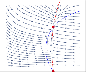
Figure 2. The phase plane for the dynamical system given by (4.2) and (4.3) for  $\mu = 1 = - 3 \lambda /2$, $Re =1$, $\mathcal {T} = 1$ and $\mathcal {Q} = 1$. From left to right the values of $\beta$ used are $\hat {\beta } = 0.1$, $\hat {\beta } = 1$ and $\hat {\beta } = 10$. Arrows indicate the trajectories of the solutions and the red disks indicate the steady states at $(\bar {\rho }, u) = (1, \mathcal {T}/(Re\mathcal {Q}))$ and $(\bar {\rho }, u) =(1, 0)$. The dashed lines illustrate the nullclines. The blue nullcline corresponds to $\partial u/\partial x = 0$ and the red nullcline illustrates where $\partial \bar {\rho }/\partial x = 0$. After crossing the nullclines, the streamlines deflect (sharply for small $\hat {\beta }$) towards the stable steady state at $(\bar {\rho }, u) = (1, \mathcal {T}/(Re\mathcal {Q}))$.
The phase planes in figure 2 can give us mechanistic insight into the role of  $\hat {\beta }$ on the trajectories in the phase plane. Smaller $\hat {\beta }$ values result in a rapid decompression (or compression for $\bar {\rho }<1$ initially) to $\bar {\rho } = 1$ without much velocity change, which is accommodated for by a increase (or decrease) in the thickness of the sheet, $h$. The length scale over which this rapid change occurs is $O(\hat {\beta }^{-1})$, which is the scaling of $x$ that gives a dominant balance between the terms in (4.3). For larger $\hat {\beta }$ values, the trajectories are more dynamic, and both $u$ and $\bar {\rho }$ can both increase and decrease on a single trajectory towards the steady state. For larger $\hat {\beta }$ values, compressibility has a more sustained influence over the evolution of the product. In the small $\hat {\beta }$ regime, compressibility influences the initial evolution of the product where the density adjusts to $\bar {\rho } \approx 1$. In the latter stage of evolution, for a small $\hat {\beta }$ value, the density remains constant and the product behaves as an incompressible fluid. The analogous incompressible scenario would be a fluid with $\bar {\rho }=1$, extruded with the same velocity, but from a die with width equal to $h=\mathcal {Q}/u$. The far-field behaviour of the fluid does not depend on $\hat {\beta }$.
Taliadorou, Georgiou & Mitsoulis (Reference Taliadorou, Georgiou and Mitsoulis2008) observed through numerical simulation that a compressible fluid will initially expand and then contract with decaying surface oscillations. Expansion and then subsequent contraction was observed in the solutions to (4.2) and (4.3) for fluids with  $\bar {\rho }>1$ initially. The fact that the eigenvalues in (4.4) are real and negative suggest that the surface does not oscillate, but instead converges exponentially to the fixed point. We have only considered unconfined flow, but the numerical simulations of Taliadorou et al. (Reference Taliadorou, Georgiou and Mitsoulis2008) included a die wall, which may be the source of the surface oscillations that they observed.
There are two special values of the second coefficient of viscosity:  $\lambda : \lambda = -2 \mu /3$, which is often chosen so that the deviatoric stress makes no contribution to the mean normal stress (Batchelor Reference Batchelor2000); and $\lambda = -3 \mu$, which we deduce from (4.2) corresponds to the nullclines of (4.2) and (4.3) coinciding. If $\lambda = -3\mu$, (4.2) is undefined away from any fixed point. However, there is currently no known real-world scenarios where we would expect $\lambda = -3 \mu$, which would correspond to a negative bulk viscosity. Thus, $\lambda = -3 \mu$ is a mathematically important case, but of no obvious practical importance.
4.2. Vapour-driven expansion
For a practically relevant example of vapour-driven expansion, we consider the manufacture of cereal and expanded snack foods. As such, in this section we close the system of equations (3.4), (3.8) and (3.9) using (3.11) and use the parameter values appropriate for cereal extrusion given by Lach (Reference Lach2006), which can be found in table 1. The corresponding Reynolds number is  $Re = 1.1\times 10^{-3}$ and the inverse capillary number is $\varGamma = 5.5 \times 10^{-5}$, which are both small; thus, we consider the consequences of neglecting terms containing these dimensionless parameters. While the reduced governing equations allow for axially varying viscosity, to simplify our discussion, we assume that the viscosity is constant for the remainder of this paper. In practice, the viscosity will depend on the nature of the mixture being extruded.
Table 1. Parameter values typical of cereal extrusion taken from Lach (Reference Lach2006). The units of  $\textrm {bubbles}/\textrm {m}^3_{liquid}$ refer to the number of bubbles per unit volume of wet cereal mixture (the liquid phase of the mixture).

For steady flow in the absence of surface tension ( $\varGamma = 0$) and inertia ( $Re = 0$), (3.4) and (3.8) may be integrated to yield
 \begin{equation} \bar{\rho} u h = \mathcal{Q}, \quad \frac{4 \mu \mathcal{Q} }{\bar{\rho}^2 u^2}\frac{\partial }{\partial x }\left( \frac{\bar{\rho} u^2}{2} \right)= \mathcal{T}, \end{equation}
where the mass flux,  $\mathcal {Q}$, and the tension in the sheet, $\mathcal {T}$, are constants. With no tension on the sheet, such as for a product being cut after extrusion, we can make further progress by integrating (4.5b). The tension in the sheet depends on the stress boundary condition at the end of the sheet. As noted earlier, we are interested in the case in which no normal stress is applied to the end of the sheet, which corresponds to $\mathcal {T}=0$.
When  $\mathcal {T}=0$, we have two conserved quantities: $\mathcal {Q}$, given by (4.5a,b), and $\mathcal {E}$, defined by
 \begin{equation} \frac{\bar{\rho} u^2}{2}=\mathcal{E}. \end{equation}
In the absence of surface tension and inertia, we can obtain an expression for the pressure by combining (3.9), (4.5a,b) and (4.6). As a result, we can present a system of equations governing the time-steady, spatial evolution of a 2-D compressible sheet in the absence of inertia and surface tension given by
 \begin{equation} \bar{\rho} u h = \mathcal{Q},\quad \frac{\bar{\rho} u^2}{2} =\mathcal{E}, \quad \bar{p} ={-}\frac{(\lambda+ \mu) u}{\bar{\rho}}\frac{\partial \bar{\rho}}{\partial x }, \end{equation}
and (3.11), which has practical relevance to cereal extrusion. The special case  $\lambda = -\mu$ sets the effective bulk viscosity of the fluid to zero in two dimensions, a result of which would be $\bar {p} = 0$; that is, without bulk viscosity, the fluid pressure is equal to atmospheric pressure as soon as it exits the extruder.
4.3. Coupled model analysis
Using (4.7a–c), we can reduce (3.11) to an ODE for the density given by
 \begin{equation} {\frac{\textrm{d} \bar{\rho}}{\textrm{d}\kern0.06em x }} ={-}\frac{3 (1 - \bar{\rho}) \bar{\rho}^{{3/2}} }{2^{5/2} \mathcal{E}^{1/2} ( 1+ 3(1 - \bar{\rho})(\lambda + \mu)/4)} \left(\frac{C \bar{\rho}}{1 - \bar{\rho}}- p_{{atm}}\right), \end{equation}
where  $\bar {\rho }_0=1/(1 + \alpha )$, with the initial volume fraction ratio of gas to liquid $\alpha = 4{\rm \pi} \eta R_0^3/3$, is the density at $x=0$ according to (2.3). Thus, we have found that with a simple microscale law and uniform inlet density the equations for a viscous compressible sheet are reduced to a single ODE. This autonomous ODE admits the implicit analytic solution
 \begin{equation} \int_{{\bar{\rho}_0}}^{\bar{\rho}}-\frac{ (2\mathcal{E})^{1/2} ( 4+ 3(1 - \bar{\rho}')(\lambda + \mu))}{3 (\bar{\rho}')^{{3/2}} (C \bar{\rho}'- p_{{atm}}(1 - \bar{\rho}'))} \,\textrm{d} \bar{\rho}' = x . \end{equation}
From (4.7) and (4.8) we can see that the sheet tends to the steady profile given by
 \begin{equation} \bar{\rho} \rightarrow \left( 1 + \frac{C}{ p_{{atm}}}\right)^{{-}1},\quad u \rightarrow \sqrt{\frac{2 \mathcal{E}}{\bar{\rho}}},\quad h \rightarrow \frac{\mathcal{Q}}{\sqrt{2 \mathcal{E} \bar{\rho}}},\quad \bar{p} \rightarrow 0 \text{ as } x\rightarrow \infty, \end{equation}
for  $C \neq 0$, which holds in all physical scenarios of relevance.
4.4. Solutions to the coupled microscale–macroscale model
We present numerical results to the system of (4.7) and (4.8) for a product cut at  $x=1$, which corresponds to the time-steady extrusion of a viscous, bubbly mixture with uniform density, $\bar {\rho }_0$, at the inlet under no tension. We consider the impact of different inlet densities on the evolution of the mixture. We also consider varying the parameter $C$, which encapsulates the thermodynamics of our simple microscale model. Here we are interested in expansion, so we take the default value of $C = 10$, as this is sufficiently large to overcome the liquid pressure surrounding the bubbles. We avoid the case $C< p_{{atm}}(1 - \bar {\rho }_0)/ \bar {\rho }_0$, where the bubble pressure at the inlet is lower than atmospheric pressure and the bubbles will collapse. The dynamics of bubble collapse are too complicated to be described by the closure relation (3.11), and a more suitable model should at least include surface tension. For illustrative purposes, we take $\mu = 1$ and $\lambda = 0$; however, in practice these parameters may depend on the state of the system.
We find it useful to compare the results for the compressible fluid to those for an incompressible fluid under equivalent conditions (i.e. under no tension). In this case, with  $\mathcal {T} = 0$, for an incompressible fluid, the variables are unchanged from their inlet values, which can be seen by setting $\partial \bar {\rho } /\partial x = 0$ in (4.7) and (4.8).
In figure 3 we illustrate  $h$,
$h$,  $\bar {\rho }$, $u$ and $\bar {R}$, the bubble radius associated with $\bar {\rho }$, for a range of $\bar {\rho }_0$ values. We see that as $\bar {\rho }_0$ is increased towards 1 (i.e. approaching the incompressible limit with no bubbles), $h$,
$h$,  $\bar {\rho }$ and $u$ tend to the equivalent constant values of an incompressible fluid. Away from this limit, for moderate values of $\bar {\rho }_0$, the change in the compressible sheet is more substantial: as the bubbles grow, we see thickening and acceleration of the sheet, and a decrease in density. An incompressible sheet cannot simultaneously thicken and accelerate; conservation of mass (4.7) forbids this. A compressible fluid, however, can both expand and accelerate as the density decreases. The most substantial bubble growth occurs for values of $\bar {\rho }_0$ closer to the incompressible limit of 1 (figure 3d), however, in this limit the bubble number density, and therefore $\alpha$, approaches zero. Hence, although more substantial bubble growth occurs, the macroscopic impact of this is negligible (figures 3a and 3c). Bubble growth is larger in this limit as the flow speed is lowest in the absence of expansion-induced acceleration, which allows more time for the bubbles to grow.

Figure 3. Half-width,  $h$, density, $\bar {\rho }$, velocity, $u$, and bubble radius, $\bar {R}$, for $\bar {\rho }_0= \{0.995, 0.975, 0.95, 0.89, 0.81\}$ corresponding to initial gas-to-liquid volume fractions of $\alpha = \{ 0.01, 0.05, 0.1, 0.25, 0.5\}$, keeping $u_0=1$, $C = 10$ and $h_0 = 1$ fixed (i.e. varying initial density). The dashed lines indicate the solution for an incompressible fluid under equivalent conditions.
By introducing a microscale model to close the flow equations, we introduced a parameter  $C$ that encapsulates the microscale thermodynamics. Larger values of $C$ correspond to higher initial bubble pressures and lead to more rapid and substantial changes in the sheet (figure 4). In the limit as $C$ approaches $p_{{atm}}(1 - \bar {\rho }_0) /\bar {\rho }_0$, the right-hand side of the evolution equation for $\bar {\rho }$ (4.8) vanishes. This solution resembles the incompressible case by remaining unchanged. However, the sheet is not incompressible; instead, the bubble pressure is in perfect balance with the liquid pressure. For $C < p_{{atm}}(1 - \bar {\rho }_0) /\bar {\rho }_0$, the bubbles will shrink.

Figure 4. Half-width,  $h$, density, $\bar {\rho }$, velocity, $u$, and bubble radius, $\bar {R}$, for $C= \{0.5, 1, 5, 10\}$, keeping $\bar {\rho }_0 = 0.9$, $u_0 = 1$ and $h_0 = 1$ fixed (i.e. varying inlet velocity).
5. Concluding remarks
In this paper we presented a reduced model for the extensional flow of a viscous compressible sheet. This model describes a general unconfined extensional flow with changing density, and was motivated by the specific need to gain a better understanding of manufacturing techniques that extrude compressible fluids. Full models for such flows have numerous challenging aspects: free boundaries, complicated governing equations and pressure–density relationships that may require integrating along fluid streamlines. The model described in this paper offers a simpler theoretical framework that can be used to understand these flows, while still providing useful information about the state of the fluid such as the sheet thickness, averaged cross-sectional density and pressure, and the flow speed.
While the equations for conservation of mass and momentum of compressible fluids typically take the same form, the additional pressure–density relationship required to close the governing equations depends strongly on the specific fluid being described. In §§ 4.1 and 4.2 of this paper we considered two extrusion problems using different closure relationships. In § 4.1 we assumed a linear relationship between the pressure and density. In this case, while only neglecting surface tension, the resulting governing equations comprised a dynamical system of two ODEs: (4.2) and (4.3). The simplicity of this reduced model meant that analytic methods (that are not applicable to the full model) could elicit useful information. For example, by analysing the phase plane we identified the steady state of the system and demonstrated that this state is linearly stable when the system is under tension. We can also gain mechanistic insight that is not obvious from the full model, such as the role of the dimensionless compressibility,  $\hat {\beta }$, on the evolution of the system and the transition from compressible to incompressible fluids for small $\hat {\beta }$.
In §§ 4.2–4.4 we demonstrated how a microscale model for bubble growth could be incorporated. This particular microscale model is a simple variant of the models used by Alavi et al. (Reference Alavi, Rizvi and Harriott2003) and Lach (Reference Lach2006) to model vapour-driven expansion during extrusion. In this case we demonstrated that the dynamics of the system were governed by a single ODE, from which it was simple to read off the far-field behaviour of the sheet.
To better understand the behaviour of a compressible sheet, a useful reference is the behaviour of incompressible sheets under equivalent conditions. The results presented in § 4.4 demonstrate that compressible and incompressible sheets will exhibit very different qualitative behaviour. One such difference is the simultaneous acceleration and expansion that can be exhibited by a compressible sheet, which is compensated for by a reduction in density. There are many interesting phenomena observed in incompressible extensional flow, such as sintering (cf. Cummings & Howell Reference Cummings and Howell1999), that are yet to be explored for a compressible flow.
The reduced model we present in this paper has both advantages and disadvantages when compared with the full model presented in § 2. While the reduced model is much simpler than the full model, this simplicity is a consequence of making a number of assumptions that may not hold for all extrusion problems. If the aspect ratio,  $\epsilon$, is not small, the neglected components of the full model will influence the dynamics, namely, the neglected stress components. Another source of model breakdown is the neglected physical processes, in particular, thermodynamics and temperature-dependent viscosities. For a multi-scale model of vapour-driven expansion, the thermodynamics is likely to have a strong influence on bubble dynamics. The methodology for including conservation of thermal energy would be very similar to that described in Taroni et al. (Reference Taroni, Breward, Cummings and Griffiths2013) for incompressible fluids, and is a sensible next step in extending this model.
The main advantage of the reduced model is the simplicity of the governing equations; the equations being ODEs rather than partial differential equations (PDEs) on a domain with a free boundary. By systematically reducing the governing equations, we have addressed the need for simpler, mechanistic models for extrusion raised by Kristiawan et al. (Reference Kristiawan, Chaunier, Della Valle, Ndiaye and Vergnes2016). A reduced model cannot be systematically derived for all compressible fluids because, even though the conservation equations can be averaged over the cross-section, it is not possible in general to systematically average the state equation. This is because the pointwise relationship between these quantities can be nonlinear, so the cross-section integrals are not possible to evaluate analytically. For the special case of a linear state equation, (1.1), a closed model for the averaged quantities can be systematically derived. For more complicated closure relationships, a constitutive model relating the cross-sectionally averaged quantities must be used.
With a reduced model for the flow of a compressible sheet, it is much easier to investigate the impact of different microscale dynamics on the macroscale flow. Incorporating a more complex microscale model, including microscale diffusive transport of mass and energy, into the reduced flow model is considerably simpler when compared with the full model. A reduced macroscale model comprising only ODEs, rather than PDEs on a freely evolving domain, drastically simplifies any analysis on the interplay between microscale dynamics and macroscale mass and momentum transport. For application to vapour-driven expansion problems, we have also assumed that the equations for single-phase compressible flow are appropriate. This will not be true of multiphase flows in general, and the single-phase flow equations are typically only employed when the bubbles are small and well dispersed.
This model is limited to cases in which the compressible sheet is free to expand. This means that, for extrusion, another model would be required to understand the behaviour of the mixture inside the extruder; the output of this model would provide inlet conditions for the reduced model presented in this paper.
The reduced model for compressible flow presented in this paper provides a simple framework with which to study real-world systems involving viscous compressible fluids. The resulting model is analogous to the Trouton model for incompressible flow and, in a similar manner, provides the base upon which more complicated dynamics can be studied.
Declaration of interests
The authors report no conflict of interest.
Appendix A. A closure relationship for microscale bubble growth
Following the approach of Brennen (Reference Brennen2005), we can construct a relationship between pressure and the rate of change of mixture density. The volume fraction of gas,  $\alpha _g$, is related to the number of bubbles per unit volume of liquid, $\eta$, and the bubble volume, $V$, by
 \begin{equation} \alpha_g = \alpha_l \eta V, \end{equation}
where  $\alpha _l$ is the volume fraction of liquid. We assume that $\eta$ is uniform in space and constant in time; that is, the bubbles in the mixture are uniformly distributed at the inlet, and we do not consider further nucleation or bubble coalescence. Since $\alpha _l+\alpha _g=1$, (A1) can be used to express $\alpha _l$ in terms of $\eta$ and $V$ as
 \begin{equation} \alpha_l = \frac{1}{1 + \eta V}. \end{equation}
The density of the mixture is given by
 \begin{equation} \rho = \rho_l \alpha_l + \rho_g \alpha_l, \end{equation}
where  $\rho _l$ is the density of the liquid component and $\rho _g$ is the density of the gas component. Here we shall assume that the density of the gas contained in the bubbles is negligible so $\rho _g \ll \rho _l$. The density of the mixture is then given by
 \begin{equation} \rho = \frac{\rho_l}{1 + \eta V}. \end{equation}
 The bubble volume is related to the radius of the bubbles,  $R$, according to $V = 4 {\rm \pi}R^3/3$. The bubble radius can be determined by the Rayleigh–Plesset equation (Rayleigh Reference Rayleigh1917; Plesset Reference Plesset1949),
 \begin{equation} \rho_l \left(\frac{\textrm{D} R}{\textrm{D} t} \right)^2 + \rho_l R \frac{\textrm{D}^2 R}{\textrm{D} t^2} = p_{{B}} - p - \frac{2 \gamma_l }{R} - \frac{4 \mu_l}{R}\frac{\textrm{D} R}{\textrm{D} t}, \end{equation}
where  $p_{{B}}$ is the pressure of the vapour in the bubble.
We non-dimensionalise (A5) by introducing the scalings
 \begin{equation} R = R_0 R', \quad p_{{B}} =\frac{\mu_l U}{L} p_{{B}}', \end{equation}
and by using the scalings introduced in § 2.2 for  $t$,
$t$,  $\boldsymbol {u}$, $\boldsymbol {x}$ and $p$. We have chosen to use the viscous pressure scaling for $p_B$ and the initial bubble radius, $R_0$, for $R$. From hereon, we only consider dimensionless variables and drop all primes. The result of this rescaling is the dimensionless Rayleigh–Plesset equation given by
 \begin{equation} Re_{{B}}\left(\frac{\textrm{D} R}{\textrm{D} t} \right)^2 + Re_{{B}} R \frac{\textrm{D}^2 R}{\textrm{D}t^2} = p_{{B}} - p - p_{{atm}} - \frac{\varGamma_{{B}} }{R} - \frac{4}{R}\frac{\textrm{D} R}{\textrm{D} t}, \end{equation}
where  $Re_{{B}}$ is the reduced microscale Reynolds number,
 \begin{equation} Re_{{B}} = \frac{\rho_l W R_0^2}{\mu_l L}, \end{equation}
and  $\varGamma _{{B}}$ is the inverse capillary number for the microscale model, given by
 \begin{equation} \varGamma_{{B}} = \frac{2 \gamma_l L}{\mu_l R_0 U}. \end{equation}
Using the parameter values in table 1 gives a typical reduced microscale Reynolds number of  $Re_{{B}} = 3.6\times 10^{-9}$ and a typical microscale inverse capillary number of $\varGamma _{{B}} = 3.2\times 10^{-2}$.
We note that the microscale Reynolds number,  $Re_{{B}}$, is smaller than its macroscale counterpart, $Re$, while the microscale inverse capillary number, $\varGamma _{{B}}$, is larger than its macroscale counterpart, $\varGamma$, but still negligible. We therefore neglect the inertial and surface-tension terms in (A7), giving the dimensionless Rayleigh–Plesset equation for a bubble surrounded by a viscous liquid,
 \begin{equation} \frac{\textrm{D}R}{\textrm{D}t} = \frac{R}{4}(p_{{B}} - p - p_{{atm}}). \end{equation}
If we were interested in bubble collapse, the surface tension should be retained as its influence will increase as the bubbles get smaller.
The bubble growth (A10) must be solved along streamlines. As a consequence of this, and of the leading-order axial velocity being uniform in the cross-section, we can deduce a special case from the governing equations. If the density (and, therefore, bubble size) is uniform in a cross-section, then (3.5) implies that the pressure will also be uniform. If the pressure, axial velocity and bubble radii are uniform in a cross-section, then by (A10) the bubbles in the cross-section will evolve at the same rate and remain equal in size. That is, if the bubble size in the cross-section is uniform initially, then it will remain so at leading order throughout the evolution of the product. In this special case, where  $R$ is uniform in the cross-section, it is much simpler to integrate (A10) over the cross-section.
Appendix B. Local analysis of the fixed point  $\bar {\rho } = 1$ and $u=0$


To understand the stability of the fixed point with  $\bar {\rho } = 1$ and $u=0$, we study the behaviour of trajectories near the fixed point. Consider the local coordinates $(\bar {\rho }', u')$, where
 \begin{equation} \bar{\rho} = 1+ \delta \bar{\rho}',\quad u = \delta u', \end{equation}
and  $\delta$ is small. Here $\bar {\rho }'$ and $u'$ evolve according to (4.2) and (4.3),
 \begin{gather} \frac{\textrm{d} u'}{\textrm{d}\kern0.06em x} = \frac{ (1 + \delta \bar{\rho}') u'}{4 \mu \left( 1 + \dfrac{\mu}{2 \mu + \lambda}\right) }\left({-}Re u' + \frac{\mathcal{T}}{\mathcal{Q}} + \frac{2 \mu \bar{\rho}}{\hat{\beta} (2 \mu + \lambda)(1 + \delta\bar{\rho}') u'} \right)\colon = g(\bar{\rho}', u'), \end{gather}
 \begin{gather}\delta \frac{\textrm{d} \bar{\rho}'}{\textrm{d}\kern0.06em x} = \frac{-(1 + \delta \bar{\rho}')}{ u' (2\mu + \lambda)}\left(2 \mu g(\bar{\rho}', u') +\frac{ \bar{\rho}'}{\hat{\beta}} \right), \end{gather}
where  $g(\bar {\rho }', u')$ has been defined to make the following discussion more compact.
There are two length scales associated with this system: a length scale of  $O(\delta )$ for which $u'$ is constant, and an order one length scale. Formally, a matched asymptotic expansion can be used to analyse this system; however, we are only interested in the stability properties of the fixed point at $\bar {\rho }=1$ and $u=0$, so we opt for a more concise description.
Over the  $O(\delta )$ length scale, we can introduce $X = x/\delta$, where $X$ is order 1 as $\delta \rightarrow 0$. From (B3), at leading order in $\delta$, we find that $u'$ is a constant and $\bar {\rho }'$ tends to a steady state given by
 \begin{equation} 2 \mu g(\bar{\rho}', u') ={-}\frac{\bar{\rho}'}{\hat{\beta}} \implies \bar{\rho}' = \bar{\rho}^* ={-}\frac{\mathcal{T} \hat{\beta} (\lambda + 2 \mu)u'}{ \mathcal{Q} (\lambda + 3 \mu)}. \end{equation}
 Over the longer length scale, we have  $\bar {\rho }' = \bar {\rho }^*$, and at leading order in $\delta$ we have
 \begin{equation} \frac{\textrm{d} u'}{\textrm{d}\kern0.06em x} = \frac{\mathcal{T} (\lambda + 2 \mu)u'}{4 \mathcal{Q} \mu (\lambda + 3 \mu)}. \end{equation}
For  $\mathcal {T} >0$, $\lambda + 2 \mu >0$ and $u'>0$, we have $\textrm {d} u'/\textrm{d}\kern0.06em x > 0$. Thus, after a rapid convergence of $\bar {\rho }'$ towards $\bar {\rho }^*$, the velocity increases and the trajectories diverge from the fixed point at $u=0$ and $\bar {\rho }=1$. So, the fixed point is an unstable saddle node, because trajectories rapidly approach along the $\bar {\rho }$ axis, and then deflect towards the stable node at $\bar {\rho } =1$ and $u = \mathcal {T}/(Re \mathcal {Q})$.
Appendix C. Extention of microscale model to account for mass exchange
We present a system of equations that can be used to extend the microscale model presented in § 2.1 to account for changes in the amount of gas in the bubbles. We consider the presence of a blowing agent in the liquid surrounding the bubbles that can vaporise at the liquid–bubble interface. To account for the evolution of  $N$, we extend the existing microscale model given by (2.5) and (2.6).
On the microscale we have a gas bubble of radius  $R$, whose evolution is given by (2.4), and a liquid in $r>R$, where $r$ is the radial coordinate in the microscale coordinate system, as illustrated in figure 5. In the liquid phase we assume there is a dissolved gas of concentration $c(r, t)$, where $r > R$ and $t\geq 0$ is the time since nucleation. To integrate this model with the macroscale model, we need to transform from the Lagrangian frame of the bubble to the Eulerian frame of the extruded fluid.

Figure 5. Schematic of an ideal gas bubble surrounded by a liquid of infinite extent. In the liquid phase we must account for the transport of mass and momentum; as well as dissolved-gas transport. At the interface between phases we impose boundary conditions associated with conservation of mass, conservation of momentum and thermodynamic equilibrium.
The rate at which the dissolved species vaporises into the bubble is given by
 \begin{equation} \frac{\textrm{d}N}{\textrm{d}t} = 4{\rm \pi} R^2 D \frac{\partial c(0, t)}{\partial r}, \end{equation}
where  $D$ is the diffusion coefficient for the blowing agent in the liquid and at $t=0$ we have $N(0) = N_0$.
The concentration of the dissolved species is given by
 \begin{equation} \frac{\partial c}{\partial t} + u_r \frac{\partial c}{\partial r} = \frac{D}{r^2}\frac{\partial }{\partial r}\left(\frac{\partial c}{\partial r} \right), \end{equation}
where  $u_r$ is the radial velocity of the liquid phase in the reference frame of the bubble. We assume that the initial concentration of the dissolved species is
 \begin{equation} c(r, 0) = c_0, \end{equation}
and that
 \begin{equation} c \rightarrow c_0 \quad\text{ as }r \rightarrow \infty. \end{equation}
For the final boundary condition, at  $r=R$, we assume that the gas pressure and dissolved-gas concentration are related through Henry's law
 \begin{equation} p_B (t) = H c(R, t), \end{equation}
where  $H$ is the coefficient of Henry's law.
To non-dimensionalise the microscale model we employ the same scalings used for the macroscale model in § 2.2 and introduce the following scalings for microscale quantities:
 \begin{equation} \left.\begin{array}{c} \displaystyle r = R(0) r', \quad t = \dfrac{L}{U}t', \quad u_r = \dfrac{R_0 U}{L}u'_r,\\ \displaystyle N = \dfrac{4 {\rm \pi}R_0 D L c_0}{U}N', \quad p_{{B}} = \dfrac{\mu_l U}{\epsilon L}p'_{{B}}, \quad c = c_0 + c_0 c'. \end{array}\right\} \end{equation}
Here a prime indicates a dimensionless variable. We drop primes from hereon and only deal with dimensionless variables.
The updated dimensionless model, which was before given by (2.18) in the paper, is now given by the dimensionless Rayleigh–Plesset equation
 \begin{equation} u \frac{\partial \rho}{\partial x } + v \frac{\partial \rho}{\partial y}={-} \frac{3(1 - \rho) \rho }{4}(p_{{B}} - p - p_{atm}), \end{equation}
where the dimensionless bubble pressure is given by
 \begin{equation} p_{b} = \frac{\alpha N \rho }{1 - \rho}, \end{equation}
and  $\alpha =4{\rm \pi} R_G \epsilon L^2 T R_0 \eta D c_0 / \mu U^2$ is a dimensionless constant. The dimensionless rate of change in the amount of gas in the bubbles is given by
 \begin{equation} \frac{\textrm{d}N}{\textrm{d}t} = R^2 \frac{\partial c(0, t)}{\partial r}, \end{equation}
where  $N(0) = N_0 U/ 4 {\rm \pi}R_0 D L c_0$. The dimensionless concentration of the dissolved species is given by
 \begin{equation} \frac{\partial c}{\partial t} + u_r \frac{\partial c}{\partial r} = \frac{1}{Pe\, r^2}\frac{\partial }{\partial r}\left(\frac{\partial c}{\partial r} \right), \end{equation}
where  $Pe = R_0^2 U/D L$ is the Péclet number. The initial concentration of the dissolved species is
 \begin{equation} c(r, 0) = 0, \end{equation}
and the boundary conditions are given by
 \begin{equation} c \rightarrow 0 \quad\text{ as } r \rightarrow \infty, \end{equation}
and
 \begin{equation} p_B (t) = \beta (1 + c(R, t)), \end{equation}
where  $\beta =\epsilon L H c_0 /\mu _l U$ is a dimensionless constant.
To integrate this microscale model with the macroscale model, we must perform a coordinate transform from the Lagrangian frame of the bubble to the Eulerian frame of the macroscale fluid. This amounts to transforming total derivatives in microscale time  $t$ to advective derivatives in the macroscale frame and integrating the microscale model along the fluid streamlines (this has already been done for the Rayleigh–Plesset equation). The evolution in the number of moles of gas (C9) is given by
 \begin{equation} u \frac{\partial N}{\partial x} + v \frac{\partial N}{\partial y} = R^2 \frac{\partial c(0, x, y)}{\partial r}, \end{equation}
in the frame of the extruded fluid. It remains to express the microscale diffusion equation (C10) in the frame of the extruder. The appropriate way to do this depends on whether the particular assumptions are valid and on the amount of analysis the user is willing to perform on this system of equations prior to transformation. For example, see the boundary layer analysis for a large Péclet number detailed by Patel (Reference Patel1980), the result of which is an ODE in time for a dimensionless concentration that can be readily transformed into the Eulerian extruder frame. This form is limited due to the additional assumptions required; in particular, the authors assume that the concentration is quadratic in the boundary layer. An approach that requires fewer assumptions is to discretise the spatial dimension of the advection–diffusion equation (C10), resulting in a system of ODEs that can be easily transformed into the frame of the extruded fluid. A complete description of this methodology is detailed by McPhail et al. (Reference McPhail, Oliver, Parker and Griffiths2019).


 Open access