


1. Introduction
Bubbles rising though a liquid is a frequently occurring situation in nature (e.g. bubble plumes rising from the bottom of a lake), daily life (e.g. bubble chains rising in carbonated drinks) and technology (e.g. waste water treatment). For the case of bubble swarms rising freely in a quiescent fluid, the bubbles tend to distribute inhomogeneously, spontaneously forming clusters. When the bubbles are large enough, the rising bubbles generate turbulence in the liquid, a phenomenon referred to as bubble-induced turbulence (BIT). This BIT in turn influences the clusters and understanding this is important both for its own sake, and also due to its impact on many aspects of bubble motion, including their rise velocities, collisions, dispersion and the intensity of the BIT generated (Takagi, Ogasawara & Matsumoto Reference Takagi, Ogasawara and Matsumoto2008; Tagawa et al. Reference Tagawa, Roghair, Prakash, van Sint Annaland, Kuipers, Sun and Lohse2013; Lohse Reference Lohse2018; Liao et al. Reference Liao, Ma, Krepper, Lucas and Fröhlich2019; Ma, Lucas & Bragg Reference Ma, Lucas and Bragg2020a; Ma et al. Reference Ma, Ott, Fröhlich and Bragg2021).
Early numerical investigations (e.g. Smereka Reference Smereka1993) on bubble clustering in the presence of BIT assumed spherical bubbles and considered potential flow, and found that the bubbles form large horizontal clusters as they rise. However, subsequent experiments and more realistic numerical simulations did not clearly observe such clusters, but 2-bubble clusters with a wide range of orientations were identified as the most commonly occurring clusters (Zenit, Koch & Sangani Reference Zenit, Koch and Sangani2001; Bunner & Tryggvason Reference Bunner and Tryggvason2003; Esmaeeli & Tryggvason Reference Esmaeeli and Tryggvason2005). The prevalence of 2-bubble clusters has motivated the community to explore the dynamics of bubble pairs with varying separations and orientations, usually for the case of clean bubbles (Hallez & Legendre Reference Hallez and Legendre2011). The two extreme cases are bubbles aligned side by side (Legendre, Magnaudet & Mougin Reference Legendre, Magnaudet and Mougin2003) and in line (Zhang, Ni & Magnaudet Reference Zhang, Ni and Magnaudet2021). The results indicate that the side-by-side configuration is more stable than the in-line case, and this is because for the in-line configuration a slight transverse movement of the trailing bubble relative to the leading bubble makes it ‘feel’ a shear flow, that can drive the trailing bubble out of the leading bubble's wake. Nevertheless, stable in-line bubble chains are often observed in carbonated drinks. This contradiction was recently explained by Atasi et al. (Reference Atasi, Ravisankar, Legendre and Zenit2023) as being due to the combined effects of bubble deformation and contamination in such liquids that can result in a reversal of the lift force and stable chain. In addition to exploring the stability of nearby bubble pairs, the impact of neighbouring bubbles on their rise velocity has been investigated and compared with the case of isolated bubbles. Hallez & Legendre (Reference Hallez and Legendre2011) showed that the side-by-side configuration maximizes the drag force acting on a pair of bubbles, while the in-line bubble configuration minimizes the drag due to wake entrainment for the trailing bubble.
These studies on bubble pair dynamics have provided much insight, however, there are many open questions concerning the behaviour of bubble swarms where two or more bubbles may be clustered together, whose motion may also be affected by the wakes of other bubbles and bubble clusters in the flow. Indeed, while the rise velocity of bubble pairs in a quiescent liquid is well understood, their behaviour in the context of bubble swarms is debated. For example, the experiments of Stewart (Reference Stewart1995) and Brücker (Reference Brücker1999) for large deformable bubbles in a swarm found that the mean rise velocity was considerably larger than that for a single bubble. However, this contradicts other experimental (Ishii & Zuber Reference Ishii and Zuber1979) and numerical (Roghair et al. Reference Roghair, Lau, Deen, Slagter, Baltussen, Annaland and Kuipers2011) studies for large bubbles, which argue that the mean bubble rise velocity decreases monotonically as the gas void fraction is increased.
Several fundamental questions remain mostly unexplored: What is the probability of forming clusters involving  $N_b$ number of bubbles? What is the lifetime of these clusters? How does the rise velocity of bubbles in a cluster depend on $N_b$? How do the answers to these questions depend on contaminants in the liquid? In this paper we explore these questions experimentally by tracking thousands of deformable bubbles in a vertical column, using a recently developed machine-learning algorithm to detect and follow the evolution of bubble clusters, and explore how the bubble rise velocities depend on $N_b$. We also consider the effect of surfactants to provide a more complete picture for real systems where contaminants may cause behaviour that differs substantially from that of an idealized clean system.
2. Experimental method
2.1. Experimental set-up
The experimental apparatus is identical to that in Ma et al. (Reference Ma, Hessenkemper, Lucas and Bragg2022), and we therefore refer the reader to that paper for additional details; here, we summarize. The experiments were conducted in a rectangular bubble column (depth 50 mm and width 112.5 mm), with a water fill height of 1000 mm (figure 1). Air bubbles are injected through 11 spargers which are homogeneously distributed at the bottom of the column.

Figure 1. Sketch of the bubble column used in the experiments (note that, in the actual experiment, the number of bubbles in the column is  $O(10^3)$). The sketch is not to scale. The insets show the cylindrical cluster search region: view from (a) the top, (b) the side and (c) the front. Note that (a,b) are only schematic representations, showing possible bubble arrangements, while (c) shows a cut from a recorded snapshot. The green outline refers to bubbles that are considered inside the sharp centre region.
We use tap water in the present work as the base liquid and consider two different bubble sizes by using spargers with different inner diameters. Note that the tap water will already be slightly contaminated prior to adding the surfactants or salts, and the bubbles can behave differently in this tap water compared with that in a pure water system (Craig, Ninham & Pashley Reference Craig, Ninham and Pashley1993; Takagi & Matsumoto Reference Takagi and Matsumoto2011). For the bubble sizes considered in the present study (with  $d_b>2$ mm), however, the slight contamination in the tap water does not have a significant effect on the bubble shape/motion, as confirmed by our previous studies (Hessenkemper et al. Reference Hessenkemper, Ziegenhein, Rzehak, Lucas and Tomiyama2021; Ma et al. Reference Ma, Hessenkemper, Lucas and Bragg2023). For each bubble size, we manipulate the gas flow rate and ensure that all cases are not in the heterogeneous regime of dispersed bubbly flows. In total, we have six mono-dispersed cases (see supplementary movies 1–6 available at https://doi.org/10.1017/jfm.2023.807) labelled as SmTapLess, SmTap, SmPen+, LaTapLess, LaTap and LaPen+ in table 1, including some basic characteristic dimensionless numbers for the bubbles. Here, ‘Sm/La’ stand for smaller/larger bubbles, ‘Pen+’ stands for corresponding cases added by 1000 ppm 1-Pentanol and ‘Less’ stands for lower gas void fraction than **Tap/**Pen+ cases for smaller/larger bubbles, respectively. It should be noted that the three cases with larger bubble sizes have higher gas void fractions than the three cases with smaller bubbles. This is because in our set-up it is not possible to have the same flow rate for two different spargers while also maintaining a homogeneous gas distribution for mono-dispersed bubbles. Furthermore, the bubble size is slightly reduced when adding 1-Pentanol for both types of sparger. This is due to the influence of the surfactants that reduce the surface tension and hence affect the bubble formation at the rigid orifice.
Table 1. Selected characteristics of the six bubble swarm cases. Here,  $\alpha$ is the averaged gas void fraction, $d_b$ the equivalent bubble diameter, $\chi$ the aspect ratio, $L_b$ the inter-bubble distance, $Ga\equiv \sqrt {|{\rm \pi} _\rho -1|gd_{b}^{3}}/\nu$ the Galileo number and $Eo\equiv \Delta \rho gd_b^2/\sigma$ the Eötvös number. The bubble Reynolds number $Re_b$ and drag coefficient $C_D$ are based on $d_b$ and the bubble to fluid relative velocity.

To identify and track bubble clusters, we use planar shadow images obtained by recording the flow with a high-speed camera and illuminating the set-up with a LED. The measurement resolution in time and space are 250 f.p.s. and 59.9  $\mathrm {\mu }$m Px $^{-1}$, respectively, with a field of view (FOV) of $90\,\mathrm{mm}\times 76\ \mathrm {mm}$. For each case, we record 1000 sequences with each having 70–75 frames – approximately the time in which a bubble passes through the complete image height.
2.2. Bubble identification and tracking
In our study one camera is used and as such the bubbles can be identified and tracked only in two dimensions. However, as will be shown in § 2.3, we are nevertheless able to identify bubble clusters in quasi-three dimensions. Independent of the number of cameras used, the task to track bubbles in image sequences can be done in a detect-to-track or in a track-to-detect fashion. While the former links previously detected bubbles in each frame to form suitable tracks, the latter uses extrapolations of already established tracks to detect bubbles in follow-up images. We use the former detect-to-track strategy, which allows us to incorporate detections among multiple frames to establish tracks with, however, relying more strongly on an accurate detector that finds bubbles in individual frames.
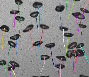
Even for low gas volume fractions, detecting bubbles in individual images is a challenging task since bubbles can overlap in the images. Fully overlapping bubbles cannot be detected, but partially overlapping bubbles can be dealt with and deep-learning-based strategies for this have recently shown very promising results (e.g. Kim & Park Reference Kim and Park2021). In our previous work (Hessenkemper et al. Reference Hessenkemper, Starke, Atassi, Ziegenhein and Lucas2022), we developed such an approach that used a trained convolutional neural network (CNN) to segment overlapping bubbles. Furthermore, the contour of each detected bubble is reconstructed using 64 radial vectors pointing from the segmentation centre to the boundary (figure 2a), and the radial vectors of partly occluded bubbles are corrected using an additional multi-layer perceptron (MLP).

Figure 2. Initialization of the tracking algorithm. (a) Cut out snapshots of three different time steps, with three detected bubbles and their reconstructed radial vectors highlighted in colour. The dashed lines indicate possible connections of the right most bubble at  $t_1$ to the successive time steps $t_2$ and $t_3$. (b) Illustrates a constructed graph with all possible connections of these three bubbles.
The subsequent tracking of multiple detected bubbles in close proximity poses further challenges, as the tracker not only has to be robust against inaccuracies of the detector, i.e. missing or false detections, but also has to be able to track bubbles that are fully occluded even for multiple times steps, while at the same time having numerous possible associations in the near vicinity. To solve these issues, a graph-based tracking formalism is used. Specifically, we follow the framework of Brasó & Leal-Taixé (Reference Brasó and Leal-Taixé2020), utilizing multiple MLPs to predict valid connections of detections on graph structured data. The four main aspects of this tracking framework are described as follows. Details on the network architectures and the training dataset are provided in Appendix A.
Graph construction: to track the bubbles, each sequence is modelled as a graph, with detections (bubbles) being the nodes of the graph and possible connections in time being the edges of the graph, i.e. a pair of detections forward or backward in time that are possibly from the same bubble (figure 2b). The task is then to classify the edges into active and non-active edges, which at the end form a set of valid tracks that fulfil the so-called ‘flow conservation constraints’ – each node having an active edge to at most one node forward in time and at most one node backward in time.
Feature encoding: for both the nodes and the edges of the graph, features are encoded with two separate MLPs (figure 3a). The node embeddings represent the appearance features of the detections, which are usually encoded with a CNN (Brasó & Leal-Taixé Reference Brasó and Leal-Taixé2020). However, monochromatic bubble images show few distinct features, with the size and the shape of the bubble image being the most relevant ones. Thus, we have chosen the 64 radial vectors from the bubble detector as input for the node feature encoder, providing not only a more accurate description of the features bubble size/shape, but also a better two-dimensional (2-D) bubble contour in the case of overlapping bubbles due to the additional correction of the radial locations. The edge embeddings represent tracking-related features. For each detected pair of frames, the time increment, relative coordinate and size are fed into the edge feature encoding MLP to generate edge embeddings.

Figure 3. Steps of the tracking algorithm: (a) feature encoding with node encoder MLP (NE) and edge encoder MLP (EE) together with edge update MLP (EU); (b) time-aware node update MLP (NU) with past node update MLP (PNU) and future node update MLP (FNU); (c) predicted active edges.
Message passing network: the core of the tracking algorithm is the message passing network (MPN) whose main purpose is to update node and edge embeddings with respect to their surrounding nodes and edges in the graph, and this is done iteratively using message passing steps. First, the edge embeddings are updated by combining their embeddings with the embeddings of the adjacent pair of nodes and feeding them into an edge-update MLP (figure 3a). Then, a time-aware node update step is applied by aggregating edge embeddings of adjacent edges, which already contain information of connected nodes due to the previous edge update step. The time awareness is introduced by first aggregating and updating separately incoming edges, i.e. connections backward in time, and outgoing edges, i.e. connections forward in time, with individual MLPs and then concatenating the outcome to finally update the node embeddings with a node update MLP (figure 3b). For each iteration, information of nodes one step further in time is passed through the network to the node/edge to be updated. Thus, the number of iterations defines the time increment of the information of other nodes that are supplied to the current node.
Edge classification and post-processing: after updating all node and edge embeddings with the MPN, the edges are classified with a classifier MLP (figure 3c). The predictions are post-processed and remaining violations of the flow conservation constraints are treated with an exact rounding scheme (Brasó & Leal-Taixé Reference Brasó and Leal-Taixé2020). Lastly, missing links in the trajectories are interpolated using bilinear interpolation and each trajectory is smoothed with a uniform filter. In supplementary movie 8 we provide qualitative results of the tracking algorithm applied on a sequence of case LaTapLess, while in Appendix B quantitative results are provided with the use of common multi-object tracking metrics. The results demonstrate that the algorithm can track the majority of the detected bubbles, with a slight performance decrease with increasing bubble size and increasing number of bubbles.
2.3. Identification and tracking of bubble clusters
The detection of bubble clusters at each time step follows a distance criterion between neighbouring bubbles whose centres in the 2-D image domain are below a predefined threshold  $2d_b$ from each individual case (figure 1c). This value is mainly based on the work of Legendre et al. (Reference Legendre, Magnaudet and Mougin2003) that a considerable drag enhancement is observed for a bubble pair rising side by side within this distance. Tests for different thresholds ( $2d_b\pm 0.5d_b$) were conducted and the trends of the results in § 3 were found to be insensitive to the choice of this parameter. Furthermore, since we attempt to detect the bubble cluster in a quasi-3-D manner, we keep the in-focus region in the depth direction to also be $2d_b$ (figure 1a,b). To estimate this depth distance to the centre plane we use the grey value gradient of the detected bubbles and consider only sharp bubbles in the shallow depth of field (DoF) region (see Appendix C for more detail). In summary, we utilize a cylindrical search volume, ${\rm \pi} (2d_b)^2\times 2d_b$, for the cluster identification, radial in the 2-D image domain and linear in the depth direction. For all the cases, the mean inter-bubble distance $L_b$ based on the global void fraction (table 1) is much larger than the search radius $2d_b$, indicating that the bubble clusters to be discussed are dynamically significant.
The cluster tracking strategy is inspired by the work of Liu et al. (Reference Liu, Shen, Zamansky and Coletti2020) for characterizing the temporal evolution of inertial particle clusters in turbulence. Considering two clusters identified in two consecutive time steps ( $\Delta t=1/250$ s), we take both to be successive realizations of the same cluster if the number of bubbles they share is above a given threshold. The shared bubbles across clusters in successive time steps are termed connections. We consider forward-in-time and backward-in-time connections, and apply thresholds on the fraction of connected bubbles over the total number of bubbles in each cluster. We illustrate in figure 4(a) an example: cluster A (identified in time step 1) shares all its bubbles with cluster C (identified in time step 2), while C shares 2/3 of its bubbles with A. Therefore, the fractions of forward and backward connections between A and C are 1 and 2/3, respectively. On the other hand, B shares 1/3 of its bubbles with C, and C shares 1/3 of its bubbles with B. Thus, the forward and backward connections between B and C are 1/3 and 1/3, respectively. Following Liu et al. (Reference Liu, Shen, Zamansky and Coletti2020), two clusters in consecutive time steps are identified as the same cluster when the fractions of their backward and forward connections are both $\geq 1/2$. In the example of figure 4(a), A and C are recognized as belonging to the same cluster. The cluster lifetime is defined as the time elapsed between birth (the first instance a cluster is identified) and death (the last time it is recognized). Here, we explicitly include the lower threshold of $1/2$, since many 2-bubble clusters appear and require an additional criterion for tracking. In figure 4(b) we give an example where cluster A at time step 2 splits into B and C. To decide whether B or C should be regarded as the continuation of cluster A for the purposes of tracking, we consider whether cluster B or C persists longer into the future. In this example, while cluster C survives until time n, B does not. Therefore, we regard C, D and A as belonging to the same cluster, while cluster B is considered to be a newborn cluster at time step 2. This approach eliminates ambiguities since it ensures that a cluster at any instant can only be associated with at most one cluster either in the past or future.

Figure 4. Method of tracking clusters: (a) illustrates an example of two clusters merging into one cluster; (b) illustrates an example of one cluster separating into two clusters.
3. Results
3.1. Probability of being clustered
We first consider the percentage of bubbles in the flow that are clustered based on the data points listed in table 2. The results in figure 5(a) show that this percentage increases in the order of SmTapLess, SmTap to SmPen+ for the smaller bubbles. While the increase from SmTapLess to SmTap is quite understandable due to the increase of the gas void fraction, the result from SmPen+ (whose  $\alpha$ is sightly less than that of SmTap) shows that the surfactant promotes the formation of clusters. We obtained similar results for the three cases with larger bubbles (figure 5b).
Table 2. Number of bubbles tracked and number of clusters in the FOV used for computing the statistics.


Figure 5. Percentage of bubbles in cluster for the cases with smaller (a) and larger (b) bubbles. Probability of number of bubbles within a cluster for the different cases using linear (c) and log (d) plot, respectively.
In figure 5(c,d) we consider the probability of finding a given number of bubbles within a cluster for all cases, plotting the results using both linear and logarithmic vertical axes in order to highlight regions of both high and low probability, respectively. The results show that the probability decreases with increasing  $N_b$ and, consistent with previous studies, $N_b=2$ is the most common cluster size for all 6 cases (Zenit et al. Reference Zenit, Koch and Sangani2001; Bunner & Tryggvason Reference Bunner and Tryggvason2003). However, the results also show that $N_b=3,4$ clusters occur with non-negligible probability, and there are even rare events with $N_b=8$ clusters. The results also show that adding contaminants decreases the probability of forming $N_b=2$ clusters, and increases the probability of forming larger clusters, although the dependence is not too strong. For a fixed contaminant level, increasing $\alpha$ has the same effect.
3.2. Lifetime
We now turn to consider the mean lifetime of the clusters,  $\langle t_{life}\rangle$, as a function of $N_b$ (only the results for $N_b\leq 5$ are shown as the statistics for $N_b>5$ are not converged). Figure 6(a,b) shows $\langle t_{life}\rangle$ normalized by a characteristic time scale of BIT (Ma et al. Reference Ma, Santarelli, Ziegenhein, Lucas and Fröhlich2017, Reference Ma, Lucas, Jakirlić and Fröhlich2020b), $t_{BIT}\equiv d_b/U_b$, where $U_b$ is the mean vertical slip velocity between the bubble and liquid at the column centre. The values of $\langle t_{life}\rangle /t_{BIT}$ are order unity, suggesting that $t_{BIT}$ is indeed a dynamically relevant time scale for the cluster lifetimes. The results also reveal a systematic dependence on $N_b$ and the liquid contamination. First, $\langle t_{life}\rangle$ decreases monotonically with increasing $N_b$, such that larger bubble clusters are not only rarer (see § 3.1), but also more unstable. While this may not seem surprising, it is in fact the opposite to what has been observed for inertial particles where the cluster size and its lifetime are positively correlated (Liu et al. Reference Liu, Shen, Zamansky and Coletti2020). The difference could be simply due to the fact that the most common values of $N_b$ for our clusters are much smaller than those for the inertial particles in Liu et al. (Reference Liu, Shen, Zamansky and Coletti2020), and as a result relatively small changes in the bubble configurations can result in the formation or destruction of a given cluster. The other significant difference is that our bubbles hydrodynamically interact, unlike the numerically simulated inertial particles in Liu et al. (Reference Liu, Shen, Zamansky and Coletti2020), where a one-way coupling assumption is used. Second, increasing $\alpha$ not only leads to the formation of larger clusters, but also slightly longer mean lifetimes for the clusters, although the lifetimes for $N_b=2$ are the least sensitive to $\alpha$. Third, the mean lifetimes of the bubble clusters notably increase with increasing contamination levels. In a recent paper we showed that increased contamination leads to a reduction of $Re_b$ and an increase in BIT (Ma et al. Reference Ma, Hessenkemper, Lucas and Bragg2023). The reduction in $Re_b$ causes the bubble trajectories to be less chaotic, and this may explain why the cluster lifetimes increase with increasing contamination.

Figure 6. Mean lifetime of 2-, 3-, 4- and 5-bubble clusters (a,b) and PDF of the bubble cluster lifetime (c,d) for smaller bubble cases (a,c) and larger bubble cases (b,d).
Figure 6(c,d) shows the probability density functions (PDFs) for the cluster lifetimes, which have been computed using clusters of all sizes. The general dependence on the flow variables is similar to that observed for the mean cluster lifetime, with the PDF tails becoming increasingly heavy in the order TapLess, Tap and Pen+ for both the small and large bubbles. The majority of the bubble clusters survive for  $t_{life}/t_{BIT}=O(1)$, however, there are extreme cases where clusters survive for up to $t_{life}/t_{BIT}\approx 15$ for the Pen+ cases. Such extreme cases reflect the strongly nonlinear and non-equilibrium nature of the flow, with large fluctuations about the mean-field behaviour being an essential feature of turbulent flows. The central regions of the PDFs are approximately described by stretched exponential functions, however, the range of $t_{life}$ over which this applies is quite small.
3.3. Mean  $N_b$-bubble cluster rise velocity

We finally consider the role that clustering plays in the mean bubble rise velocity. Figure 7 shows the mean rise velocity of bubbles in clusters  $U_b$ conditioned on $N_b$, and the results for unclustered bubbles $N_b=1$ are also shown for reference. Consistent with our previous results based on averaging over all bubbles (Ma et al. Reference Ma, Hessenkemper, Lucas and Bragg2023), the results show that, for almost all $N_b$, increasing the liquid contamination leads to a reduction in $U_b$, due to the modification of the bubble boundary conditions. For the larger bubbles we also observe a clear increase in $U_b$ with increasing $N_b$, with an increase of up to $20\,\%$ when going from unclustered bubbles ( $N_b=1$) to bubble pairs ( $N_b=2$), while the increase is more moderate when $N_b$ is increased beyond 2. The enhancement of $U_b$ when going from $N_b=1$ to $N_b=2$ is also observed in the SmPen+ case, with only slight enhancements when $N_b$ is increased beyond 2. However, for the SmTapLess and SmTap cases, $U_b$ varies only weakly with $N_b$, even in going from $N_b=1$ to $N_b=2$.

Figure 7. Mean bubble rise velocity as a function of the number of bubbles  $N_b$ in the cluster: (a) smaller bubbles and (b) larger bubbles. Here, $N_b=1$ denotes unclustered bubbles.
What is the physical explanation for why the clustered bubbles rise faster than unclustered bubbles? We begin by considering the case of bubble pairs  $N_b=2$ and plot in figure 8 the mean inclination angle $\theta$ of the bubble pair centreline with respect to the vertical direction (see sketch in the figure). (It should be noted that, since our measurements are only quasi-three-dimensional, $\theta =0$ does not necessarily mean that the bubbles are in line because they may nevertheless be separated in the depth direction by up to a distance $2d_b$.) For all cases an almost uniform distribution of $\theta$ is observed, i.e. there is no preferential alignment for a bubble pair. This is consistent with visual inspection of the experimental images (see supplementary movies) which show that the bubble pair orientations are not persistent, but instead the bubbles continually trade places in a ‘leapfrog’ fashion. This observation was also found in many 3-D experiments (Stewart Reference Stewart1995; Riboux, Risso & Legendre Reference Riboux, Risso and Legendre2010) and direct numerical simulation for bubble swarms (Bunner & Tryggvason Reference Bunner and Tryggvason2003; Esmaeeli & Tryggvason Reference Esmaeeli and Tryggvason2005). It is, however, strikingly different from the behaviour observed for isolated bubble pairs where a stable configuration is observed for two clean spherical bubbles where they rise side by side (Hallez & Legendre Reference Hallez and Legendre2011), while for contaminated systems their stable configuration is in line due to the lift reversal experienced by the trailing bubble (Atasi et al. Reference Atasi, Ravisankar, Legendre and Zenit2023). From the standpoint of our experiment, several possible reasons might explain this discrepancy. First, compared with the case of spherical bubbles, a pair of deformable bubbles that are hydrodynamically interacting are likely to generate an asymmetric flow which could destabilize their configuration. Second, in our experiments the bubbles have oscillating and/or chaotic rising paths, for which the probability that two bubbles will rise in a stable arrangement is very low. By contrast, in Hallez & Legendre (Reference Hallez and Legendre2011) the bubbles are fixed at various positions, and in Atasi et al. (Reference Atasi, Ravisankar, Legendre and Zenit2023) $Re_b$ is small enough such that the bubbles have straight rising paths. Third, the bubble pairs in our experiments are not isolated. Given the present bubble sizes/void fractions, they can experience fluctuations and turbulence due to the wakes of other bubbles in the flow, and this will readily suppress any preferential orientation that might have occurred were the bubble pairs isolated.

Figure 8. Orientation of bubble pair for the different cases (e.g. in-line bubble pair for  $\theta =0^\circ$ and side by side for $\theta =90^\circ$).
Although the bubble pair orientation is almost random, the impact of their interaction on  $U_b$ will, however, depend on $\theta$, especially in the present bubble regime (deformable bubbles with $Re_b\sim O$(100–1000)). For example, in the side-by-side configuration the two bubbles are outside of each other's wakes and the modification to the drag force on each bubble is minimal (Kong et al. Reference Kong, Mirsandi, Buist, Peters, Baltussen and Kuipers2019). On the other hand, for the in-line configuration the trailing bubble is sheltered by the leading bubble and the reduced pressure behind the leading bubble causes the trailing bubble to be sucked towards it, increasing the rise velocity of the trailing bubble while the leading bubble is almost unaffected (Zhang et al. Reference Zhang, Ni and Magnaudet2021). Consequently, two mechanisms are in competition: one is vortex interaction (for relatively large $\theta$) and the second is BIT, i.e. wake entrainment (for smaller $\theta$). These effects mean that only the rise velocity of trailing bubbles will be significantly affected by the clustering, and hence, when averaged over all orientations, the increased vertical velocity of the trailing bubbles leads to an overall increase in $U_b$. This explains the increased mean rise velocity for $N_b=2$ compared with the $N_b=1$ results in figure 7. The increase is, however, minimal for the cases SmTapLess and SmTap. This is most likely due to the bubble wakes being weaker for these cases, a result of which is that the bubble interaction and the associated effect on $U_b$ is also weaker.
The results in figure 7 show that  $U_b$ further increases as $N_b$ is increased beyond 2. This can be understood in terms of the enhanced opportunity for bubbles to be sheltered by other bubbles as $N_b$ increases. However, the increase when going from $N_b=2$ to $N_b=3$ is not as strong as when going from $N_b=1$ to $N_b=2$ because the greatest effect of sheltering will occur when all the bubbles in the cluster are in line, and the probability of the bubbles in an $N_b=3$ cluster all being in line will be less than that for the bubbles in an $N_b=2$ cluster being in line. It is interesting to note that for experiments on heavy particles settling in a quiescent fluid, similar behaviour was also found, with clustered particles falling faster (Huisman et al. Reference Huisman, Barois, Bourgoin, Chouippe, Doychev, Huck, Morales, Uhlmann and Volk2016). In that case, the enhanced settling velocity was also attributed to a sheltering effect, i.e. reduced drag on particles that are falling in the wake of other particles. However, in that context, the particle clusters were found to exhibit strong alignment with the vertical direction, unlike our bubble clusters whose orientations are almost random (at least for the $N_b=2$ case).
3.4. The PDF of $N_b$-bubble cluster rise velocity fluctuations

More detailed information about the bubble rise velocities is provided in figure 9, where PDFs of the fluctuating rise velocity  $u_b=\tilde {u}_b-U_b$ (where $\tilde {u}_b$ is the instantaneous vertical bubble velocity) of bubbles in an $N_b$-bubble cluster are shown. Only results up to $N_b=3$ are shown since the results for $N_b>3$ are very noisy.

Figure 9. The PDFs of the fluctuating rise velocity of bubbles in an  $N_b$-bubble cluster, normalized by their standard deviations $\sigma _{u_b}$, with $N_b = 1, 2, 3$ for all the six cases: (a) SmTapLess, (b) SmTap, (c) SmPen+, (d) LaTapLess, (e) LaTap and (f) LaPen+.
The PDFs for all cases are asymmetric, and in particular are negatively skewed, especially for the three smaller bubble cases. This is consistent with the observations in Martínez et al. (Reference Martínez, Chehata, van Gils, Sun and Lohse2010) for a bubble swarm rising in still water, and also with a recent study for a single bubble rising in a flow with background turbulence (Ruth et al. Reference Ruth, Vernet, Perrard and Deike2021). The latter study is relevant to our experiments since any bubble rising in a swarm experiences a turbulent flow due to the turbulence generated by the surrounding bubbles. Other previous studies, however, show contrasting results for the PDF shapes. Riboux et al. (Reference Riboux, Risso and Legendre2010) used optical probes to measure the bubble velocity and found its vertical fluctuation was positively skewed. They argued the vertical bubble velocity fluctuations are controlled by the vertical liquid velocity fluctuations which have a positive skewness. In our previous study (Ma et al. Reference Ma, Hessenkemper, Lucas and Bragg2022) we also found that, for dispersed bubbly flows, the vertical liquid velocity fluctuations were positively skewed, but here we find the opposite skewness for the bubble velocities. Loisy & Naso (Reference Loisy and Naso2017) simulated a single bubble interacting with homogeneous isotropic turbulence and found that the PDF of the bubble vertical velocity fluctuations was approximately Gaussian. They argued that a skewness of either sign in the PDF of the bubble vertical velocity fluctuations is possible, depending in a complex manner on the background turbulence and presumably on other factors such as the bubble size compared with the turbulence length scales. For example, a trailing bubble located in the wake of a leading bubble would predominantly experience a positive upward liquid velocity due to the wake entertainment effect. On the other hand, the counterflow generated between bubbles leads to a downwards liquid motion that balances the flow being entrained into the bubble wakes. If other bubbles are in these downward regions it could lead to an enhancement of their negative fluctuating velocity. The skewness of the bubble rise velocity fluctuations therefore depends in a complex way on how the bubbles interact with the flow field generated by other bubbles in their vicinity.
4. Conclusions
We conducted experiments on the temporal evolution of bubble clusters with the aid of a new bubble tracking method for crowded swarms. Our results show that 2-bubble clusters are the most common, however, 3- and 4-bubble clusters also often occur. The clusters persist on average for a time of order  $d_b/U_b$, although rare clusters persisting for an order of magnitude longer are also observed. Furthermore, surfactants are observed to enhance the cluster sizes and their lifetimes. A positive correlation between cluster size and bubble rise speed is observed, with clustered bubbles rising up to $20\,\%$ faster than unclustered bubbles. We investigated the mean inclination angle $\theta$ of a bubble pair and found that, for all cases, $\theta$ has an almost uniform distribution. However, the impact of the inclination on the bubble rise velocities is different for different $\theta$. For instance, the in-line configuration is expected to have a higher impact on the bubble rise velocity compared with the side-by-side configuration.
We also investigated the PDFs of the fluctuating rise velocities of bubbles in clusters of varying sizes. The PDFs for all cases are asymmetric, and in particular are negatively skewed, especially for the three smaller bubble cases.
Finally, while our cluster tracking method is only quasi-three-dimensional, a fully 3-D method for dense, deformable bubbles can be developed by combining our bubble identification method with the recent tracking algorithm of Tan, Zhong & Ni (Reference Tan, Zhong and Ni2023) that currently applies to spherical bubbles.
Supplementary movies
Supplementary movies are available at https://doi.org/10.1017/jfm.2023.807.
Acknowledgements
T.M. would like to acknowledge P. Shi for valuable discussion for § 3.3.
Declaration of interests
The authors report no conflict of interest.
Data and code availability
The data that support the findings of this study are available from T.M. and H.H. on request. The software and trained model are available from https://rodare.hzdr.de/record/2317.
Author contributions
T.M and H.H. contributed equally to this work.
Appendix A. Network and training details
As stated in the main text, the tracking algorithm uses 7 jointly trained MLPs for the tasks feature encoding, updating edge and node embeddings and edge classification. The final network architecture of all used MLPs is shown in figure 10. We performed several hyperparameter variations, like number and sizes of hidden layers, optimizer and learning rate, with only minor changes to the final result. During the hyperparameter optimization we found that the graph size is crucial, since a too small graph may not provide the desired tracking of missed/occluded objects over multiple frames, while too bloated graphs are too hard to train. To limit the graph size and consequently the number of in-going and out-going connections, the graph is split into subgraphs of length 10 frames, with 9 overlapping frames between successive subgraphs. In the post-processing step these subgraphs are combined so that objects are still tracked along the complete sequence length.

Figure 10. The MLP structures and layer sizes of the used network. Here, FC denotes a fully connected layer.
To train the network, we created a new dataset, which consists of semi-artificial image sequences, in which single bubble tracks are overlaid on top of each other so that the ground truth is known and no labelling is required. The single bubbles were tracked in additional measurements and an image cut out along the bubble contour was saved for each time step. Then the images of several single bubble tracks were placed in an empty background image with a random starting position either inside or below the image to let bubbles rise inside the image region. For overlapping bubbles the contour of the bubble in front is slightly darkened to incorporate the shadow effect of the bubble behind. With this strategy we created in total 36 sequences of different length, different f.p.s., different number of bubbles and with different bubble sizes in the range of 2–7 mm. An example of such a semi-artificial sequence is provided in supplementary movie 7.
One drawback of this strategy is that the bubble tracks do not show any possible effects of close-by bubbles, bubble–bubble interactions or substantially different background flows. To still enable an accurate tracking under such conditions, considerable data augmentation is applied, as introduced by Brasó & Leal-Taixé (Reference Brasó and Leal-Taixé2020), including random position shifts, randomly dropping detections, i.e. increasing the number of missing detections, and random f.p.s. changes.
Appendix B. Validation
To test the performance of the tracking algorithm, 4 additional semi-artificial image sequences were generated in the same manner as the training sequences. In the field of multi-object tracking, several metrics exist that can be used to quantify the goodness of the algorithm, emphasizing different tracking aspects. To evaluate the tracker accuracy we use multi object tracking accuracy (MOTA), defined as
 \begin{equation} {\rm MOTA}=1-\frac{\displaystyle\sum_t (m_t+fp_t+mme_t)}{\displaystyle\sum_t g_t}, \end{equation}
with  $m_t$ being the number of misses, $fp_t$ the number of false positives, $mme_t$ the number of mismatches, i.e. ID switches, and $g_t$ the number of ground truth objects at time $t$. The MOTA thus comprises the sum of the three error sources: ratio of misses, ratio of false positives and ratio of mismatches, and is independent of the precision of the estimated object position. This latter attribute is captured with the multi object tracking precision (MOTP), defined as
 \begin{equation} {\rm MOTP}=\frac{\displaystyle\sum_{i,t} d_{i,t}}{\displaystyle\sum_t c_t}, \end{equation}
with  $d_{i,t}$ being the intersection over union distance for the $i$th match and $c_t$ the number of matches (Bernardin, Elbs & Stiefelhagen Reference Bernardin, Elbs and Stiefelhagen2006). Table 3 shows the results for the 4 validation cases together with further tracker metrics and information on the cases. Note that inaccuracies of the detector are already present in the results. Here, $U_b^\varepsilon =U_b^g-U_b^{det}$ denotes the error of the determined average bubble rise velocity as the difference between ground truth velocity $U_b^g$ and determined velocity $U_b^{det}$ of the tracker. The results demonstrate the capability of the tracker to track multiple bubbles in swarms, with a slight dependency on the bubble number and size. The bubble number for the real measurements presented in the main text lies in the range 100–200 bubbles per frame, for which the tracking algorithm shows a high accuracy and hence ensures a stable tracking of bubble clusters. A demonstration of tracked bubbles in a real measurement is provided in supplementary movie 8.
Table 3. Performance evaluation of the tracker. Here,  $\langle tp\rangle$ denotes the average number of true positives per time step.

Appendix C. Depth distance estimation
In order to identify bubble clusters in a quasi-3-D manner, we use the grey value gradient along the bubble contour as a sharpness measure to define whether two bubbles are in the narrow DoF region and therefore also have a sufficiently small distance in the depth direction. To accurately determine the depth position of a bubble, we conducted additional stereoscopic measurements with two cameras of single bubbles rising in the same set-up. Figure 11(a,d) shows the grey value gradient in dependence on the depth position for numerous smaller and larger bubbles with similar sizes as the Sm and La cases. The large variation is mainly due to illumination inhomogeneities and noise, whereby larger bubbles show more variations due to the narrow DoF. A simple thresholding would lead to large errors, as indicated in figure 11(b,e). Here, the ground truth shows all bubbles that are actually within the search boundary of  $2d_b$, while the coloured dots show all bubbles that would be considered to be within the search boundary. To overcome the inaccuracies of using a threshold, we use a radial basis function (RBF) to estimate the distance of a bubble from the focal plane. Specifically, we use the RBFInterpolator of the python package scipy (Fasshauer Reference Fasshauer2007; Virtanen et al. Reference Virtanen2020) with a thin plate spline RBF. As input for the RBF, we use the mean of the grey value gradient of all contour points defined by the end of the radial distances that do not touch neighbouring bubbles, as well as the bubble size and its 2-D location in the front view image to further account for size effects and illumination inhomogeneities. Approximately 32 000 bubble images from the stereoscopic measurements were used for training and 8000 bubble images for testing the accuracy of the RBF approach. With this RBF method, more bubbles within and less bubbles outside the search boundaries are predicted in comparison with the threshold method as shown in figure 11(c,f). Quantitatively, this is captured in table 4, where the precision and recall of both methods are compared.

Figure 11. Depth estimation calibration: grey value gradient relation to depth position (a,d) and predicted bubbles within search boundary for the threshold method (d,e) and RBF method (c,f) for small bubbles  $d_b\approx 3$ mm (a–c) and large bubbles $d_b\approx 4$ mm (d–f).
Table 4. Performance evaluation of the depth estimation method.

To further reduce errors of the depth estimation, we smooth the predicted depth along the track. This is illustrated in figure 12, where the unsmoothed prediction would falsely predict three distances out of the search boundary, which is not the case for the smoothed distance. This smoothing is only possible when sharp and unsharp bubbles are tracked before predicting and filtering based on the centre plane distance.

Figure 12. Depth estimation of a tracked 4 mm bubble oscillating around the centre plane.


 Open access