


1. Introduction
The stratification established by turbulent miscible plumes within sealed containers of fluid (the so-called ‘filling box’ after Baines & Turner Reference Baines and Turner1969) or containers in which the interior connects to an exterior environment via openings (the ‘emptying–filling box’ after Linden, Lane-Serff & Smeed Reference Linden, Lane-Serff and Smeed1990) has garnered considerable interest given the range of buoyancy-driven stratified flows in the manmade and natural environments that fall into these categories. Examples of filling boxes in the natural environment include underground chambers supplied by magma plumes (Campbell & Turner Reference Campbell and Turner1989) and ocean basins stratified by aqueous plumes (Wong, Griffiths & Hughes Reference Wong, Griffiths and Hughes2001). Our focus herein concerns the aptly named emptying–filling box, for which buoyant fluid is supplied to and simultaneously empties from the box – the latter via openings in the base and top that link the interior and exterior environments.
The wide range of possible variations in box geometry and in the manner in which buoyancy is supplied results in a myriad of different emptying–filling box configurations. We consider the flow patterns and stratifications established by two buoyancy sources of differing strengths where one source is elevated relative to the other. This configuration covers scenarios of practical interest including indoor spaces with multiple occupied levels, such as atria, mezzanines and tiered auditoria. In contrast to the large area distributed buoyancy sources considered by Livermore & Woods (Reference Livermore and Woods2007), we address the flow patterns resulting from localised buoyancy sources that give rise to turbulent plumes. The predictions of our theoretical model (§ 2), backed up by complementary flow visualisations and density measurements (§ 5), reveal this to be a rich and complex problem in which a multiplicity of distinct flow regimes are possible.
Mathematical descriptions of emptying–filling box flows have been developed to predict the steady stratification established by turbulent plumes rising from single or multiple localised buoyancy sources at the same elevation with identical strengths (Linden et al. Reference Linden, Lane-Serff and Smeed1990) and for sources with different strengths (Cooper & Linden Reference Cooper and Linden1996; Linden & Cooper Reference Linden and Cooper1996, hereafter Reference Cooper and LindenCL96 and Reference Linden and CooperLC96). The transient flows that lead to a steady state are of considerable interest due to the complex behaviours they exhibit, including interface and thermal overshooting phenomena and sidewall overturning motions (Baines & Turner Reference Baines and Turner1969; Kaye & Hunt Reference Kaye and Hunt2004, Reference Kaye and Hunt2007; Bower et al. Reference Bower, Caulfield, Fitzgerald and Woods2008; Shrinivas & Hunt Reference Shrinivas and Hunt2014a). Herein the transients have been tracked during experiments solely to confirm that a unique steady flow is reached, irrespective of the order in which the plume sources are activated – a key result on which our complementary steady-state theoretical analysis relies. The transient processes by which plumes create layers that evolve towards steady thicknesses and homogeneous densities is detailed elsewhere (e.g. Baines & Turner Reference Baines and Turner1969; Linden et al. Reference Linden, Lane-Serff and Smeed1990; Kaye & Hunt Reference Kaye and Hunt2004). Our focus hereinafter is exclusively on steady flows, on sources that produce turbulent plumes and on boxes with openings to the exterior in the base and top.
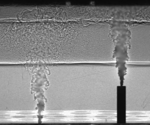
In the absence of plume–plume or plume–sidewall interactions, Reference Cooper and LindenCL96 postulate that two buoyancy sources of unequal strengths that are located at an identical elevation produce a three-layer stratification (comprising homogeneous upper, intermediate and lower layers each separated by horizontal interfaces). For the case of positive buoyancy sources producing rising plumes, the stronger plume supplies the upper layer, the weaker plume the intermediate layer, and the lower layer is comprised of fluid drawn in from the exterior through the base opening (figure 1a). In addition to this basic arrangement, they modelled two secondary processes: a downward vertical transport of fluid caused by the impingement of the weaker plume on the upper interface, and the change in plume entrainment due to the reduction of buoyancy flux in the stronger plume as it enters the intermediate layer. These processes raised the height of the upper interface relative to the predictions made if neglected (figure 1b). Flow visualisations, such as the shadowgraph (figure 1c) from our experimental campaign (§ 5), confirm the general appropriateness of their theoretical conceptualisation.

Figure 1. (a) With both buoyancy sources on the box base, the plume with greater buoyancy flux forms the upper layer and the weaker plume forms the intermediate layer. (b) The coupling between plume and stratification results in two secondary effects: vertical transport of fluid from the upper to the intermediate layer of volume flux  $Q_{I}^*$, and a modification of the entrainment into the stronger plume within the intermediate layer. These secondary effects increase the height of the upper interface. (c) Flow visualisation showing two buoyant layers and the impingement of the weaker plume (left) on the upper interface (experiment 43, § 5).
Building on the analysis of Reference Cooper and LindenCL96, Reference Linden and CooperLC96 considered the more complex case of  $n \geq 2$ equal-elevation plume sources. It was demonstrated by Reference Linden and CooperLC96 that accounting for the aforementioned reduction of the plume buoyancy flux in the stratification is not necessarily important. Neglecting both of the secondary processes, their simplified model provided a robust prediction of the stratification created by $n$ sources and offered design guidance for naturally ventilated buildings with multiple localised floor-level heat sources. In § 2 we initially adopt a similar approach by neglecting these secondary processes so as to develop an analytical model for the more complicated general case where two sources are at distinct elevations.
The remainder of this paper is structured as follows. The analytical model is presented in three parts, commencing in § 2 with the theoretical framework that includes a description of the flow structure and the associated governing equations for six distinct flow regimes. In § 3 we consider the limiting behaviour in each regime to identify the regime boundaries and reveal the dependence on the relative elevations of the two sources, the ratio of the source strengths and the resistance of the box to emptying. Regime boundaries are not straightforward to identify a priori and the regime maps we develop aid in determining which regime prevails for a given set of parameters and, hence, which governing equations are appropriate. There are stark differences between regimes in stratification and flow behaviour, and some example predictions are shown in § 4. In § 5 we describe the experimental campaign conducted to measure the stratification and provide confirmation of the predicted regimes. The campaign broadly affirms the predictions of the analytical model, and the flow visualisations reveal the significance of plume-induced mixing. This mixing results in a seventh regime as well as two mechanisms for vertical transport of fluid across a density interface, one of which concerns previously unreported mixing near the top of the box. Incorporating phenomenological models for the observed mixing into a more sophisticated model (§ 6) yields qualitative and quantitative improvements in stratification predictions. A brief discussion section (§ 7) considers some practical implications of our findings, including the potential merits of introducing an elevated heat source in a room in order to provide a cooler environment for occupants below. Finally, our conclusions are drawn in § 8.
2. Theoretical framework
We consider the range of possible steady stratification regimes that are established in an emptying–filling box by the turbulent plumes that originate from two localised buoyancy sources of differing strength and elevation. The ‘base’ and ‘elevated’ sources are located inside the box at the vertical coordinates  $z=0$ and $z=k(\geq 0)$ with positive buoyancy fluxes $B_1$ and $B_2$, respectively. Both sources have zero volume and momentum flux.
The horizontal cross-sectional area of the box is independent of height and sufficiently large that the plumes are far away from each other and the walls, and thus, their vertical development is unaffected by the lateral confinement or plume–plume interaction. Similarly, the flow through the base openings (of total area  $a_b$) and the top openings (of total area $a_t$) is assumed to have a negligible effect on plume development. The vertical distance between the base source and the top is equal to the box height $H$. We assume the plumes establish a stratification in the box consisting of one or two horizontal buoyant layers. Given the plumes cannot stratify the region below the lower source, a simple vertical offset in source elevation transforms cases where both sources are elevated to a configuration where the lower source can be treated as if on the base of the box.
Buoyant fluid rises through openings at the top at a flow rate  $Q_n$ and, simultaneously, an inflow of fluid from a quiescent exterior of constant and uniform density is drawn through openings in the base. We restrict our analysis to cases for which the inflowing fluid does not mix with the buoyant layer(s) and unidirectional outflow is maintained at the top opening(s). These restrictions are routinely assumed for emptying–filling box models and the resulting flow is referred to as a displacement flow – the incoming fluid displacing, rather than mixing with, the buoyant fluid in the interior. Hunt & Coffey (Reference Hunt and Coffey2010) developed the constraints on the opening areas, layer depths and layer buoyancies that ensure displacement flow and, broadly speaking, this flow is expected for $a_t/a_b\lesssim 3$ for circular openings.
Three possible displacement flow configurations with a three-layer stratification are sketched in figure 2. The layers are delineated by the first and second interfaces at heights  $h_1$ and $h_2$, respectively. The buoyancy of the upper, intermediate and lower layers are denoted $g'_2$, $g'_1$ and $g'_e$, respectively. Given we define buoyancy relative to the exterior density, $g'_e=0$. The plume volume flux $Q_{ij}$ at a given interface is identified by two integer subscripts, the first subscript identifies the plume source and the second identifies the interface – so, for example, $Q_{21}$ is the volume flux of the elevated plume at the level of the first interface. Each distinct flow configuration is referred to as a regime, and the three-layer regimes A3, B3 and C3 are distinguished by whether the elevated plume source supplies the intermediate layer (regime A3, figure 2a) or the upper layer (regimes B3 and C3), and whether the elevated source is below the first interface (regime B3, figure 2b) or above it (regime C3, figure 2c). We also identify three two-layer stratifications (referred to as regimes A2, B2 and C2, figure 3).

Figure 2. The idealised three-layer flows for (a) regime A3, (b) regime B3 and (c) regime C3. The horizontal dashed lines represent steady interfaces delineating layers of uniform buoyancy.

Figure 3. The idealised two-layer flows for (a) regime A2, (b) regime B2 and (c) regime C2.
Whilst, in general, a three-layer stratification might be anticipated with two plume sources, there are three physical explanations for the formation of only two layers. First, the source conditions can be such that the average buoyancy in each plume is identical at the height of the lower interface, a scenario discussed further in § 3.1.1 and that may be regarded as a limiting case of regimes A3 and B3 rather than novel behaviour. Second, the plumes can mix the upper portion of the box with sufficient vigour such that only a single well-mixed buoyant layer forms; this mixing is incorporated into the extended model (§ 6), but not the analytical model discussed at present. Third, the opening areas can be so large and, thus, provide so little resistance to flow through them that only a single buoyant layer forms, as idealised in the sketches of the two-layer regimes in figure 3. Regimes A2, B2 and C2 are similar to their three-layer counterparts, with the exception that the plume that was supplying the upper layer with buoyancy  $g'_2$ now rises to the top of the box, and fluid from this plume exits without forming this layer. In the two-layer regimes the total flow rate through the upper openings ( $Q_n$) is the sum of the volume flux of the exiting plume and the flow rate $Q_\omega$.
This third mechanism is not necessarily obvious and, indeed, Reference Cooper and LindenCL96 were seemingly only partially aware of it in their analysis of emptying–filling boxes with two plume sources. When accounting for mixing in the box, Reference Cooper and LindenCL96 explained that the second interface was pushed upwards and, depending on the opening areas and source conditions, predicted that it would reach the top of the box. At this point, they claimed that one of the plumes would reach the top of the box and exit immediately, without forming the third layer. However, they did not comment that their model also predicted that the second interface would reach the top of the box if the openings were large enough without the need for any mixing: governing systems of equations in both Reference Cooper and LindenCL96 and Reference Linden and CooperLC96 have non-physical solutions where the second interface is predicted to be above the height of the box. Two of the key theoretical developments of this paper are the wider recognition of this mechanism, which applies in any emptying–filling box with multiple buoyancy sources with sufficiently large openings, and a more detailed description and model for how one of the plumes can exit the box without forming a layer.
Having described the idealised stratifications, the analysis proceeds by considering conservation of volume and buoyancy. At steady state,  $h_1$ and $h_2$ are constant, and the net volume flux into any layer must be zero. Applying continuity for the three-layer regimes:
 \begin{equation} \underbrace{Q_n=Q_{11}+Q_{21}=Q_{12}}_{\textit{Regime A3}}, \quad \underbrace{Q_n=Q_{11}+Q_{21}=Q_{22}}_{\textit{Regime B3}}, \quad \underbrace{Q_n=Q_{11}=Q_{22}}_{\textit{Regime C3}}. \end{equation}
For the two-layer regimes,
 $$\begin{gather} \underbrace{Q_n = Q_{11} + Q_{21} = Q_{12} + Q_\omega}_{\textit{Regime A2}}, \quad \underbrace{Q_n = Q_{11} + Q_{21} = Q_{22} + Q_\omega}_{\textit{Regime B2}}, \end{gather}$$
 $$\begin{gather} \underbrace{Q_n = Q_{11} = Q_{22} + Q_\omega}_{\textit{Regime C2}}. \end{gather}$$
Conservation of buoyancy requires that the layers have uniform buoyancy and
 \begin{equation} \underbrace{g'_2=\frac{B_1+B_2}{Q_n}}_{\textit{Three-layer regimes}}, \quad \underbrace{g'_1=\frac{B_2}{Q_{21}}}_{\textit{A regimes}}, \quad \underbrace{g'_1=\frac{B_1}{Q_{11}}}_{\textit{B & C regimes}}. \end{equation}
 The buoyant layers drive a flow rate  $Q_L$ that is determined by balancing the pressure drop associated with the flow entering and exiting the box with the difference in hydrostatic pressure between the openings (cf. Linden et al. Reference Linden, Lane-Serff and Smeed1990). On determining the pressure drop through the openings using Bernoulli's equation, it is readily shown that
 \begin{equation} Q_L=A^*\left(\int_0^H g'(z)\,\mathrm{d} z\right)^{1/2} \ \textrm{with `effective area'}\ A^* = \left( \frac{1}{2c_t^2 a_t^2} + \frac{1}{2c_b^2 a_b^2} \right)^{{-}1/2}, \end{equation}
where  $c_t$ and $c_b$ are coefficients associated with the top and base opening areas, respectively, incorporating the effects of the vena contracta and any frictional losses.
In the three-layer regimes the flow through the openings results solely from the hydrostatic pressure force from the buoyant layers, and evaluating the integral in (2.4) gives
 \begin{equation} Q_n=Q_L=A^*\sqrt{g'_2(H-h_2)+g'_1(h_2-h_1)}. \end{equation}
In regimes A2, B2 and C2, one plume exits the box directly and, thus, the layer-driven component accounts for only the portion  $Q_\omega$ of the flow through the top opening(s) (figure 3). It is not obvious how the combination of these two flows should be best modelled, so we propose that the layer-driven flow occupies a proportion $\varOmega$ $(0<\varOmega <1)$ of the effective area. Accordingly, in the two-layer regimes,
 \begin{equation} Q_\omega=Q_L=\varOmega A^*\sqrt{g'_1(H-h_1)}. \end{equation}
Furthermore, we propose that  $\varOmega =Q_L/Q_n$ such that the layer-driven flow uses a fraction of $A^*$ in proportion to its contribution to the total flow rate $Q_n$ (this proposal is consistent with the layer-driven flow using the areas $a_b$ and $a_t$ in this same proportion and the coefficients $c_t$ and $c_b$ remaining unmodified). This proposal implies that
 \begin{equation} Q_n=A^*\sqrt{g'_1(H-h_1)}, \end{equation}
a relationship which is identical to the form for the displacement flow driven by the two-layer stratification resulting from a single plume (cf. Linden et al. Reference Linden, Lane-Serff and Smeed1990), and may have been expected from the outset. Indeed, Reference Cooper and LindenCL96 use this form without discussion of how the exiting plume affects the layer-driven flow. It is also a particularly appealing form for modelling purposes as the resulting solutions (§ 4) for quantities such as  $h_1$ and $Q_n$ are continuous at the boundaries between the two- and three-layer regimes. The associated assumption that $c_t$ and $c_b$ are unchanged ensures that $A^*$ is only a function of the box geometry rather than the flow conditions. We note that a similar assumption is made in many emptying–filling box models, regardless of the presence of an exiting plume, where the known variation of $c_t$ with layer thickness and buoyancy (Hunt & Holford Reference Hunt and Holford2000) is neglected for simplicity.
In reality, we expect that  $c_t$ and $\varOmega$ would vary depending on the flow conditions at the opening(s) at the top of the box, and, in particular, the position of the exiting plume in relation to the opening(s). One could imagine differences in flow behaviours for two limiting geometries: an exiting plume directly beneath a large opening such that the plume simply flows through it or, conversely, a plume impinging on the top of the box and forming a buoyant outflow current that flows to the opening(s) before exiting. However, we do not speculate herein on the significance of possible differences in these flow behaviours and, to avoid including the horizontal positions of the sources and openings in the model, treat these flows identically. Our complementary experiments (§ 5) were conducted in a box where the plume sources and openings were not vertically aligned and these confirmed that (i) a two-layer stratification can form even if the exiting plume impinges on the top of the box and (ii) that predictions for $h_1$ in experiments with a two-layer stratification based on (2.7) are very good. Accordingly, it seems that the simple proposed model for the layer-driven flow in the presence of the exiting plume for a two-layer stratification is not unreasonable.
In principle, it would be possible to have an opening so large that both plumes exit without forming a layer, yielding the trivial solution of one unstratified layer. This scenario is not explicitly modelled herein – indeed, it does not include the filling aspect of the emptying–filling box – although we note that two-layer solutions can approximate this scenario with an arbitrarily thin buoyant layer above a region at ambient density comprising nearly all of the box height.
For all regimes in the simplified model, we follow Reference Linden and CooperLC96 in neglecting the effects of the stratification on the plume volume flux and, thus,
 \begin{equation} Q_{11}=C_QB_1^{1/3}h_1^{5/3}, \quad Q_{12}=C_QB_1^{1/3}h_2^{5/3}, \quad Q_{22}=C_QB_2^{1/3}(h_2-k)^{5/3}, \end{equation}
where  $C_Q=(6\alpha _{p}/5)(9\alpha _{p}/10)^{1/3}{\rm \pi} ^{2/3}$ is the coefficient for the normalised plume volume flux and $\alpha _{p}$ is the top-hat entrainment coefficient of a plume (cf. Morton, Taylor & Turner Reference Morton, Taylor and Turner1956). Based on the van Reeuwijk & Craske (Reference van Reeuwijk and Craske2015) summary of experimental and direct numerical simulation data, we take $\alpha _{p}=0.13$. When modelling regimes A2, B2 and C2, $h_2=H$. If the elevated plume source is above the first interface, $Q_{21}=0$, and
 \begin{equation} Q_{21}=C_QB_2^{1/3}(h_1-k)^{5/3} \quad \textrm{for } h_1\geq k. \end{equation}
Defining the non-dimensional quantities
 \begin{align} \zeta_1=h_1/H, \quad \zeta_2=h_2/H, \quad \phi=k/H, \quad \psi=B_2/B_1 \quad \text{and} \quad R=C_Q^{3/2}H^2/A^*, \end{align}
the following relationship for the behaviour in regime A2 is obtained on combining (2.3), (2.1a{–}c), (2.7), (2.8) and (2.9):
 \begin{equation} \textrm{Regime A2:} \quad R=\sqrt{\frac{\psi(1-\zeta_1)}{\psi^{1/3}(\zeta_1-\phi)^{5/3}(\zeta_1^{5/3}+\psi^{1/3}(\zeta_1-\phi)^{5/3})^2}}. \end{equation}
The quantity  $R$ represents the relative resistance of the box to the plume-driven flow through the openings: increasing the plume volume flux (by increasing $C_Q$ or $H$) or reducing $A^*$ results in higher velocities and, hence, pressure losses, at the openings. Alternatively, $R$ can be regarded as the ratio of a characteristic plume volume flux $Q_p=C_QB_1^{1/3}H^{5/3}$ to a characteristic layer-driven volume flux through the openings $Q_O$ where the typical layer buoyancy is taken as $B_1/Q_p$:
 \begin{equation} R=\frac{Q_p}{Q_O}=\frac{Q_p}{A^*\sqrt{H B_1/Q_p}}=\frac{C_Q^{3/2}H^2}{A^*}. \end{equation}
As continuity requires that the actual plume and layer-driven volume fluxes be equal in a given stratification, then larger values of  $R$ imply that deeper layers are required to sufficiently reduce the sum of the plume volume fluxes at the interfaces below the characteristic value. Conversely, smaller values of $R$ imply shallower buoyant layers (to reduce the layer-driven volume flux below its characteristic value), and, for sufficiently small values of $R$, only one buoyant layer is required. Combining (2.1), (2.3), (2.5), (2.8) and (2.9) leads to the following pair of governing equations for regime A3:
 \begin{align} \textrm{Regime A3:} \quad & \zeta_2^{5/3}=\zeta_1^{5/3}+\psi^{1/3}(\zeta_1-\phi)^{5/3}, \end{align}
 \begin{align} & R=\sqrt{\frac{(1+\psi)(1-\zeta_2)+\psi^{2/3}\left(\dfrac{\zeta_2}{\zeta_1-\phi}\right)^{5/3} (\zeta_2-\zeta_1)}{\zeta_2^5}}. \end{align}
The governing equations for regime B, obtained by manipulation of (2.1)-(2.9), are
 \begin{align} \textrm{Regime B2:} \quad & R=\sqrt{\frac{1-\zeta_1}{\zeta_1^{5/3}(\zeta_1^{5/3}+\psi^{1/3}(\zeta_1-\phi)^{5/3})^2}}, \end{align}
 \begin{align} \textrm{Regime B3:} \quad & \psi^{1/3}(\zeta_2-\phi)^{5/3}=\zeta_1^{5/3}+\psi^{1/3}(\zeta_1-\phi)^{5/3}, \end{align}
 \begin{align} & R=\sqrt{\frac{(1+\psi)(1-\zeta_2)+\psi^{1/3}\left(\dfrac{\zeta_2-\phi}{\zeta_1}\right)^{5/3} (\zeta_2-\zeta_1)}{\psi(\zeta_2-\phi)^5}}. \end{align}
Similarly, for regime C,
 \begin{align} \textrm{Regime C2:} \quad & R=\sqrt{\frac{1-\zeta_1}{\zeta_1^5}}, \end{align}
 \begin{align} \textrm{Regime C3:} \quad &\zeta_1^{5/3}=\psi^{1/3}(\zeta_2-\phi)^{5/3}, \end{align}
 \begin{align} & R=\sqrt{\frac{(1+\psi)(1-\zeta_2)+(\zeta_2-\zeta_1)}{\zeta_1^5}}. \end{align}
We note that the governing equation for regime C2 is identical to the equation for an emptying–filling box with a single plume source on the base; thus, changing the properties of the elevated source has no effect on the stratification (provided the changes do not result in a switch of regimes).
3. Regime boundaries
By considering the limiting behaviour for each regime, we identify which regime occurs for a given combination of  $\psi$, $\phi$ and $R$. The appropriate governing equation(s) from (2.11)–(2.20) can then be solved for $\zeta _1$ and, if applicable, $\zeta _2$. The plume volume fluxes at each interface can then be determined via (2.8)–(2.9) and these values used to calculate $g'_1$ and $g'_2$ via (2.3), and $Q_n$ via (2.1) or (2.2), as appropriate.
3.1. Boundaries of the A regimes
3.1.1. Boundary between the A and B regimes
The crossover between the A and B regimes occurs when the buoyancy of the base plume is equal to that of the elevated plume at the first interface, i.e. when  $B_1/Q_{11}=B_2/Q_{21}$. Substitution of (2.8)–(2.9) into this condition shows that it is met if
 \begin{equation} \zeta_1=\frac{\phi}{1-\psi^{2/5}} \quad \textrm{for} \ 0<\phi<1 \quad \textrm{or} \quad \psi=1 \ \textrm{for} \ \phi=0. \end{equation}
If both buoyancy sources are on the base, then the relative strength of the plume sources alone determines which regime prevails, with  $\psi =B_2/B_1 > 1$ resulting in a B regime. For ${\phi \neq 0}$, substitution of (3.1) into either the governing equations for regime A2 (2.11) or regime A3 (2.13)–(2.14) shows that the boundary between the A and B regimes is defined by
 \begin{equation} R_{AB}=\frac{(1-\psi^{2/5})^{2}}{1+\psi}\sqrt{\frac{1-\psi^{2/5}-\phi}{\phi^5}} \quad \textrm{for} \ 0<\phi<1, \end{equation}
where  $R_{AB}(\psi,\phi )$ is the critical value that delineates the A and B regimes. If ${\psi ^{2/5}+\phi > 1}$ then $R_{AB}$ has an imaginary component and an A regime cannot occur; the buoyancy in the elevated plume will exceed the buoyancy in the base plume for any interface height $\phi <\zeta _1 < 1$. If $R < R_{AB}$ then an A regime will exist while if $R > R_{AB}$ then a B or C regime will occur. If $R=R_{AB}$ (or $\phi =0$ and $\psi =1$) then both plumes will reach $\zeta _1$ with the same average buoyancy. Consequently, no further stratification above $\zeta _1$ is possible, and thus, the boundary between the A and B regimes is characterised by a two-layer stratification.
3.1.2. Boundary between regimes A2 and A3
The boundary between regimes A2 and A3 can be found by substituting the condition  $\zeta _2=1$ into (2.13)–(2.14). After simplification, this shows that
 \begin{equation} R_{A23}=\sqrt{\frac{\psi(1-\zeta_1)}{1-\zeta_1^{5/3}}} \quad \textrm{for}\ 1=\zeta_1^{5/3}+\psi^{1/3}(\zeta_1-\phi)^{5/3}, \end{equation}
where  $R_{A23}(\psi,\phi )$ is the critical value delineating regime A2 ( $R < R_{A23}$) from regime A3 ( $R > R_{A23}$). Should a given pair of $\psi$ and $\phi$ require $\zeta _1\leq \phi$ to satisfy (3.3b) then neither regime A2 nor A3 can occur irrespective of the value of $R$ (as can also be shown by considering the boundary between the A and B regimes (§ 3.1.1).
Figure 4 shows regime maps for three example values of  $\psi$. Focusing on the boundaries of the A regimes (which can only occur if $\psi < 1$), the map in figure 4(a) shows that the boundary between regimes A2 and A3 is nearly vertical (almost independent of $\phi$) and that, for most values of $\phi$, increasing $R$ results in regime A2 transitioning to regime A3, which transitions to regime B2 or B3 with further increase. However, the map also shows that there are some values of $\phi$ where $R_{A23} > R_{AB}$ and the flow will skip regime A3 and transition directly from regime A2 to B2 with increasing $R$ (e.g. $0.58 \lesssim \phi \lesssim 0.60$ for $\psi =1/10$). These qualitative boundary features are typical for regimes A2 and A3 across a range of $\psi$.

Figure 4. Regime maps in  $R-\phi$ space for (a) $\psi =1/10$, (b) $\psi =1$ and (c) $\psi =10$. Regimes A (purple), B (green) and C (blue) are delineated by dashed lines. Dotted lines delineate two-layer regimes (lighter shading) from three-layer regimes (darker shading).
3.2. Boundaries between and within the B and C regimes
The boundary between the B and C regimes is set by substituting  $\zeta _1=\phi$ into the governing equations and the boundaries within are set by substituting $\zeta _2=1$ into the three-layer governing equations. Applying both of these conditions simultaneously shows that all four boundaries intersect at a single critical point (figure 4). For a given value of $\psi$,
 \begin{equation} R_{\textit{crit}}=\sqrt{\frac{(1+\psi^{1/5})^4}{\psi}} \quad \textrm{and} \quad \phi_{\textit{crit}}=\frac{\psi}{\psi+\psi^{4/5}}. \end{equation}
Comparison to these critical values greatly assists in determining which regime will occur for a given combination of  $\psi$, $\phi$ and $R$. As is clearly shown by considering the critical points in figure 4, regime B2 cannot occur if $R > R_{\textit {crit}}$, regime C3 cannot occur if $R < R_{\textit {crit}}$, regime B3 cannot occur if $\phi > \phi _{\textit {crit}}$ and regime C2 cannot occur if $\phi < \phi _{\textit {crit}}$. Applying these conditions eliminates two possible regimes leaving two remaining possibilities (assuming that the A regimes have already been ruled out).
3.2.1. Boundary between regimes B2 and C2
This boundary should be considered if  $R < R_{\textit {crit}}$ and $\phi > \phi _{\textit {crit}}$. For both regimes B2 and C2, upon substituting $\zeta _1=\phi$, the governing equations (2.15) and (2.18) simplify to
 \begin{equation} R_{BC2}=\sqrt{\frac{1-\phi}{\phi^5}}, \end{equation}
where  $R_{BC2}(\phi )$ is the critical value delineating regime B2 ( $R < R_{BC2}$) from regime C2.
3.2.2. Boundary between regimes B2 and B3
This boundary is important if  $R < R_{\textit {crit}}$ and $\phi < \phi _{\textit {crit}}$. The boundary between regimes B2 and B3 is found by setting $\zeta _2=1$ in (2.16)–(2.17). This yields
 \begin{equation} R_{B23}=\sqrt{\frac{1-\zeta_1}{\zeta_1^{5/3}\psi^{2/3}(1-\phi)^{10/3}}}, \quad \textrm{for}\ (1-\phi)^{5/3}=\frac{\zeta_1^{5/3}}{\psi^{1/3}}+(\zeta_1-\phi)^{5/3}, \end{equation}
where  $R_{B23}(\psi,\phi )$ is the critical value delineating regime B2 ( $R < R_{B23}$) from regime B3.
3.3. Boundary between regimes B3 and C3
This boundary is important if  $R > R_{\textit {crit}}$ and $\phi < \phi _{\textit {crit}}$. For both regimes B3 and C3, upon substituting $\zeta _1=\phi$, (2.16)–(2.17) and (2.19)–(2.20) simplify to
 \begin{equation} R_{BC3}=\sqrt{\frac{(1+\psi)(1-\phi)-\phi\psi^{4/5}}{\phi^5}}, \end{equation}
where  $R_{BC3}(\psi,\phi )$ is the critical value delineating regime B3 ( $R < R_{BC3}$) from regime C3.
3.4. Boundary between regimes C2 and C3
This boundary is important if  $R > R_{\textit {crit}}$ and $\phi > \phi _{\textit {crit}}$. The boundary between regimes C2 and C3 is found by setting $\zeta _2=1$ in (2.19)–(2.20), yielding
 \begin{equation} R_{C23}=\sqrt{\frac{1-\psi^{1/5}(1-\phi)}{\psi(1-\phi)^5}}, \end{equation}
where  $R_{C23}(\psi,\phi )$ is the critical value delineating regime C2 ( $R < R_{C23}$) from regime C3.
3.5. Regime maps discussion
The links between the flow behaviour and a given set of values for  $\psi$, $\phi$ and $R$ are encapsulated in the relations (3.3)–(3.8), but are better visually communicated via the use of regime maps. The maps in figure 4 show how flow behaviour varies with $\phi$ and $R$ at different constant values of $\psi$. While the behaviour when $\psi \geq 1$ is relatively straightforward (figure 4b,c), when $\psi < 1$, the regime map effectively conveys the eight different possible transitions between regimes that can occur upon changing $\phi$ or $R$.
$R$.
As  $R$ is a function of the box geometry, $R$ may take a fixed value in practical situations. In such cases, it is instructive to consider the regime boundaries as functions of $\phi$ and $\psi$, subject to constant $R$. Figure 5 shows regime maps for some example $R$ values: $R=0.1$; $R=1$, which is of the approximate order of magnitude for a room designed to be naturally ventilated; and $R=10$. These maps show that the existence of any of the regimes is plausible in a practical scenario, particularly when considering that, in the context of a room, opening or closing a window or door could change $R$ by an order of magnitude.

Figure 5. Regime maps in  $\psi -\phi$ space for (a) $R=0.1$, (b) $R=1$ and (c) $R=10$. Regime A (purple), B (green) and C (blue) are delineated by dashed lines. Dotted lines delineate two-layer regimes (lighter shading) from three-layer regimes (darker shading).
4. Stratification predictions
Having expressed the governing equations (§ 2) for each regime and shown how to identify which regime prevails for a given set of values for  $\psi$, $\phi$ and $R$ (§ 3), we can now calculate the stratification in a general emptying–filling box with two buoyancy sources. Figure 6 shows contours of interface heights, $\zeta _1$ and $\zeta _2$, and the normalised layer buoyancies,
 \begin{equation} \widehat{g'_1}=\frac{g'_1H}{(B_1+B_2)^{2/3}} \quad \textrm{and} \quad \widehat{g'_2}=\frac{g'_2H}{(B_1+B_2)^{2/3}}, \end{equation}
as a function of  $\psi$ and $\phi$ for $R=1$ and $R=10$. Figure 7 shows contours of the quantities
 \begin{equation} \frac{g'_2}{g'_1}, \quad \hat{Q}_{n}=\frac{Q_n}{\left(B_1+B_2\right)^{1/3}H^{5/3}} \quad \textrm{and} \quad \frac{g'_2(1-\zeta_2)}{g'_1(\zeta_2-\zeta_1)}, \end{equation}
which are, respectively, the layer buoyancy ratio, the normalised flow rate through the box and the ratio of the relative importance of each buoyant layer in determining the flow rate. These contour plots reveal complex behaviours and highlight the importance of identifying the appropriate regime: note the cusps in the contours of  $\zeta _1$ at the A3–B2 and B2–B3 boundaries in figures 6(a) and 7(a), the discontinuity in $\zeta _2$ across the A–B boundary in figure 6(c,d) and the stark differences in contour spacing and shape depending on the regime.

Figure 6. Contours of constant (a,b)  $\zeta _1$, (c,d) $\zeta _2$, (e,f) $\widehat {g'_1}$ and (g,h) $\widehat {g'_2}$ as a function of $\psi$ and $\phi$ for (a,c,e,g) $R=1$ and (b,d,f,h) $R=10$. The regime map, with the same colour scheme as in figure 4, is shown in the background for reference. For results in two-layer regimes, $\zeta _2=1$ and $\widehat {g'_2}$ is undefined.

Figure 7. Contours of constant (a,b)  $\hat {Q}_{n}$, (c,d) $g'_2/g'_1$ and (e,f) $g'_2(1-\zeta _2)/(g'_1(\zeta _2-\zeta _1))$ as a function of $\psi$ and $\phi$ for (a,c,e) $R=1$ and (b,d,f) $R=10$. The regime map, with the same colour scheme as in figure 4, is shown in the background for reference.
Despite the complexity shown in figures 6 and 7, we can still make general comments on the flow behaviour. Perhaps most significantly, the value of  $R$ considerably affects both the shapes and magnitudes of the contours such that, in the context of a potential application, guidelines or advice for poorly ventilated buildings could be considerably different than for well-ventilated buildings. Also, most of the plotted quantities change with $\phi$ or $\psi$ more rapidly when in regimes B or C compared with regime A, thereby giving different routes for stratification control depending on regime.
5. Experimental campaign
Sixty-nine individual experiments with two saline sources were conducted to establish how the flow regime, the fractional interface heights ( $\zeta _1$, $\zeta _2$) and buoyancy ratio ( $g'_2/g'_1$) vary with $\psi$, $\phi$ and $R$. The campaign considered three values of $\psi$, and six values of $\phi$ and $R$, chosen to span regions of the parameter space where regime transitions were expected and subsequently observed to occur.
5.1. Experimental set-up
A clear acrylic box, of horizontal dimensions  $50\ {\rm cm} \times 50\ {\rm cm}$ and vertical height $H_{p}=30$ cm, was submerged in a freshwater-filled, glass-sided visualisation tank (1.2 m height and 2.5 m by 1.2 m in plan), as sketched in figure 8. The tank was sufficiently large such that the ambient conditions surrounding the box could be considered constant for the entire duration of each experiment. The lower face of the box had one opening of diameter $\varnothing =3$ cm and eight openings of $\varnothing =5$ cm, and these openings were selectively blocked to vary the area available for outflow $a_t$. Experiments were conducted with either the single $\varnothing =3$ cm opening or 1, 2, 3, 4 or 8 openings of $\varnothing =5$ cm. The area of the inflow openings $a_b=573$ cm $^2$ was unchanged for all experiments and distributed across $22\times \varnothing =5$ cm and $20\times \varnothing =3$ cm openings on the upper face of the box. The ratio of the inflow and outflow opening areas exceeded $3.6$ for all experiments and, as confirmed by our observations, thereby ensured unidirectional flow at the openings and avoided mixing by the inflow (cf. Hunt & Coffey Reference Hunt and Coffey2010).

Figure 8. Schematic of the experimental set-up showing the side view of the box inside the visualisation tank alongside the camera and lightbox (not to scale) and plan views of the upper and lower box faces (to scale). The view of the upper face shows the position of the two sources and the 42 inflow openings. The view of the lower face shows, in blue shading, the approximate size and position of the plume impingement regions (should the plume reach the lower face) and the locations of the outflow openings. These were selectively blocked, and the labels indicate which of the  $\varnothing =5$ cm openings were used; for example, experiments with $3\times \varnothing =5$ cm openings had the openings labelled 1–3 unblocked with the remaining blocked.
To avoid concerns regarding the appropriate value of the coefficients  $c_b$ and $c_t$ or how the effective area $A^*$ (2.4) is influenced by distributing the area over multiple openings, values of $R$ for each of the six opening configurations were determined in experiments with two sources of equal strength at the same elevation ( $\phi =0$). For this benchmark condition, which intentionally excludes any effects due to differences in source parameters, the value of $R$ was determined from the steady height of the single interface via $R=(1-\zeta _1)^{1/2}(4\zeta _1^5)^{-1/2}$, which can be derived from theoretical consideration of this special case (cf. Linden et al. Reference Linden, Lane-Serff and Smeed1990) or by substituting $\phi =0$ and $\psi =1$ into the governing equations for regime A3 (2.13)–(2.14). There is some evidence that the value of $c_b$ or $c_t$ at an opening varies with the local flow conditions, particularly the density difference between the interior and exterior, such that $A^*$ and thereby $R$ might vary between experiments even if the opening geometry is unchanged (Hunt & Holford Reference Hunt and Holford2000; Radomski Reference Radomski2009; Vauquelin et al. Reference Vauquelin, Koutaiba, Blanchard and Fromy2017). These effects are not considered further herein, and the experiments are analysed taking $R$ as one of the six benchmark values, ranging from $R=7.6$ ( $1\times \varnothing =3$ cm opening for outflow) to $R=0.40$ ( $8\times \varnothing =5$ cm openings for outflow), as indicated in tables 1 and 2.
Table 1. Parameters (source strength ratio  $\psi$, source height difference $\phi$, box resistance to emptying $R$ and source Richardson numbers $\varGamma _{0,1}$ and $\varGamma _{0,2}$ for the base and elevated plumes, respectively) and measurements (interface heights $\zeta _1$ and $\zeta _2$ and the layer buoyancy ratio $g'_2/g'_1$) for the 36 experiments with sources of nominally equal buoyancy flux. Entries for $\zeta _2$ and $g'_2/g'_1$ are given if two peaks in the gradient of the buoyancy profile could be identified. The entries in the ‘Expected’ and ‘Observed’ columns are the regimes predicted by the analytical model and observed in the experiments, respectively. If observations did not clearly show the existence of a single regime, then multiple regimes are listed in the order of best match (see Appendix B for discussion of ambiguous classifications).

Table 2. Parameters and measurements for the 33 experiments with unequal sources ( $B_1\neq B_2$). Entries follow the same convention as table 1. By symmetry, the measurements at $\phi =0$ and $\psi =2.7$ (experiments 37, 43 and 49) also apply to $\phi =0$ and $\psi =1/2.7$; from this second perspective, the ‘Expected’ and ‘Observed’ regimes are A3 (instead of B3).

Each plume source had radius  $b_0=2.5$ mm and was supplied from a constant head tank filled with saline solution of buoyancy $g'_0$, where $g'_0=g(\rho _0-\rho _e)/\rho _e$ and $\rho _0$ and $\rho _e$ denote the densities of the source saline and the freshwater environment, respectively. If the elevated source is within a buoyant layer, as for regimes C2 and C3, then the source buoyancy should instead be determined relative to the density of that layer, thereby reducing the source buoyancy flux compared with that calculated based on the definition of $g'_0$. However, this correction was not important herein given ${\rho _0-\rho _e\gg \rho _1-\rho _e}$, where $\rho _1$ denotes the density of the lower buoyant layer. Densities were measured using an Anton Paar DMA 4500 densitometer such that the source buoyancy was determined to within $1\,\%$. The source volume flux $Q_0$ was measured with a needle flow meter to within $4\,\%$. The source Reynolds numbers, based on the volume flux and diameter, were within the range 350–500, and the plumes were observed to be turbulent within two source diameters for all experiments, as expected from a nozzle based on the Cooper design (Hunt & Linden Reference Hunt and Linden2001). The base source was always on the upper face of the box, while the height of the elevated source was varied in $50$ mm increments, starting at the upper face until $50$ mm from the lower face. Virtual origin corrections were calculated for each source following the approach developed by Hunt & Kaye (Reference Hunt and Kaye2001) and the virtual sources (corresponding to zero volume and momentum flux) were 1.6–1.9 cm above the physical sources, depending on the source fluxes. The values for $H$ and $\phi$ were determined from the positions of the base and elevated virtual sources; for experiments where both sources were on the upper face, we neglect the small difference in the calculated virtual origins and report $\phi =0$. The source volume fluxes and buoyancies were chosen to set the buoyancy flux ratio as either $\psi =2.7, 1 \textrm { or } 1/2.7$ and such that each plume was near pure at source. For a pure plume, the scaled Richardson number
 \begin{equation} \varGamma_0=\frac{5}{8\sqrt{{\rm \pi} }\alpha_{p}}\frac{Q_0^2B_0}{M_0^{5/2}}=\frac{5{\rm \pi} ^2}{8\alpha_{p}} \frac{g'_0b_0^5}{Q_0^2}=1, \end{equation}
where top-hat profiles have been assumed (cf. Morton & Middleton Reference Morton and Middleton1973). The entries in tables 1 and 2 confirm that the plumes were nominally pure at source (within  $15\,\%$ of $\varGamma _0=1$) and that the variation in $\phi$ and $\psi$ about each nominal value is small (within $3\,\%$).
Experiments were initiated by simultaneously supplying saline solution to the two plume sources. Measurements of the stratification were taken after interface height(s) and the average buoyancy in the layer(s) remained invariant for a period of 300 s and, as such, were regarded as representative of the steady state. The buoyancy distribution was determined using the dye attenuation technique to measure the dilution of methylene blue dye added to the source saline (Cenedese & Dalziel Reference Cenedese and Dalziel1998; Allgayer & Hunt Reference Allgayer and Hunt2012). For these measurements, the visualisation tank was backlit uniformly by a lightbox comprising an array of closely spaced fluorescent tubes behind a translucent, diffusive acrylic sheet and the flows recorded with a CCD camera (JAI CV-M4+CL) positioned 3 m in front of the tank, aligned with the lower face of the box (figure 8). After making the buoyancy measurements, the lightbox was removed and the visualisation tank was lit by collimated light from a 35 mm slide projector for supplemental shadowgraph visualisations (with the same camera) on translucent paper placed on the front of the tank.
5.2. Diagnostics and interpretation
While the negatively buoyant saline plumes in the experiments descended vertically, further discussion and results are presented as if the plumes ascended for consistency and ease of comparison with the theoretical modelling.
Each row in figure 9 shows a shadowgraph visualisation, a time-averaged image of the buoyancy field and the gradient of the vertical buoyancy profile from a typical experiment. The vertical buoyancy profile was calculated by horizontally averaging the time-averaged buoyancy field across the width of the box, excluding the vertical strips occupied by the plumes or the physical source. Quantitative results for  $\zeta _1$ and, for three-layer stratifications, $\zeta _2$ and $g'_2/g'_1$ are summarised in tables 1 and 2, and are based on the vertical buoyancy profile and its gradient. Note that the plotted profiles (e.g. figure 9c) correspond to the camera view and, thus, include the effects of parallax; the coordinate $z$ in these plots corresponds to the front of the box with the box base at $z=0$ and the top of the box at $z=H_{p}$ (the same height as the camera). Profiles are not shown for $z\lesssim 0.1 H_{p}$ as, in this region, light reflections from edges of openings in the box base contaminated the dye attenuation measurements; this did not impact any layer measurements. Interface positions were determined from the observed profiles following a parallax correction (Appendix A).

Figure 9. (a,d,g,j,m) Shadowgraphs, (b,e,h,k,n) time-averaged buoyancy fields and (c,f,i,l,o) vertical profiles of the buoyancy gradient. The value of  $g'_*$ is such that the peak in the profile of the buoyancy gradient corresponding to $\zeta _1$ has a magnitude of unity, and the ‘No peak’ annotation on the profiles indicates the gradient continues to increase as $z/H_{p}\rightarrow 1$. Each row is an example of a different regime: (a–c) regime B2, experiment 29; (d–f) regime B3, experiment 45; (g–i) regime C2, experiment 69; (j–l) regime C3, experiment 57; (m–o) regime AB2, experiment 55.
Identifying the regime was straightforward for the majority of experiments as (i) the flow visualisations (e.g. figure 9a,b) and the gradient of buoyancy profile (e.g. figure 9c) clearly indicated whether there were one or two distinct buoyant layers, and (ii) the flow visualisations clearly showed which plume supplied a given layer. The first four rows of figure 9 show clear examples of regimes B2, B3, C2 and C3. The regime code AB2 is introduced to indicate a single buoyant layer supplied by both plume sources, as in figure 9(m–o). This two-layer regime exists as a result of plume-induced mixing that precludes a third layer forming when both plumes have similar buoyancies at  $\zeta _1$. This could be considered the practical realisation of the theoretical special case when both plumes reach $\zeta _1$ with exactly the same buoyancy (§ 3.1.1) and, as such, this regime is expected for all cases where $\psi =1$ and $\phi =0$ (table 1). The regime observations for these five experiments are indicated by a single code in tables 1 and 2, as are other experiments with similarly straightforward classifications.
Other experiments were more difficult to classify because the shadowgraphs and buoyancy measurements showed characteristics of multiple regimes. While we did investigate metrics to help characterise ambiguous cases as one regime instead of another, it seemed more appropriate to indicate the uncertainty rather than arbitrarily introduce a distinction; the observation column for these experiments lists multiple regimes in the order of best match. The codes B2/B3, B3/B2, C2/C3 and C3/C2 reflect the similar appearances of a thin upper layer and of a horizontally propagating outflow current resulting from plume impingement with the top of the box. The codes AB2/B2, B2/AB2, AB2/B3 and B3/AB2 indicate experiments where mixing in the buoyant region disrupted flow features of regimes B2 or B3, but was not sufficient to result in the uniform layer required for an unambiguous regime AB2 classification. Appendix B has further discussion and examples of these difficult to classify cases, including experiment 19 with its unique AB3 classification.
5.3. Brief analysis
In general, the experimental observations match the analytical model. Every regime except A2 was observed, consistent with expectations based on the studied ranges of  $\psi$, $\phi$ and $R$. The observations of regime AB2 for conditions where the two plumes did not reach the lower interface with the same buoyancy were not surprising; the model predicts $g'_2/g'_1\approx 1$ for these conditions and it was expected that plume-induced mixing could prevent such a weak stratification from forming or persisting. A more detailed quantitative comparison of the measurements and predictions follows in § 6.2, but we note that the agreement is generally good as the largest differences in the predicted and measured interface heights are only $0.05H$ for $\zeta _1$ and $0.16H$ for $\zeta _2$. There are some discrepancies between the observed and predicted regimes for some combinations of $\psi$, $\phi$ and $R$, but this is not unexpected given the deliberate choice to study parameter combinations that are predicted to be near regime boundaries.
The visualisations did show behaviours not included in the analytical model that may be responsible for some of the discrepancies. The shadowgraph in figure 10(a) shows evidence for two volume flux transfers across the upper interface resulting from plume-induced mixing. On the left, the ‘impinging’ plume – so named as it impinges on the upper layer – forms a turbulent mixing region on the upper interface. On the right, the ‘supplying’ plume – so named as it supplies the upper layer with volume flux  $Q_{S}$ – ascends through the layer, impinges on the top of the box and forms a region of turbulent mixing that disturbs the upper interface. These two processes result in net transfers of fluid across the upper interface at rates $Q_{I}^*$ downwards and $Q_{S}^*$ upwards, as indicated in the idealised schematic in figure 10(b). Unsurprisingly, the significance of the mixing induced by the supplying plume appears to depend on the height of the upper interface; the shadowgraphs in figure 10(c,d) show less mixing on the interface for lower $\zeta _2$. While the former impingement behaviour was described and modelled by Reference Cooper and LindenCL96 for the limiting case $k=0$, the additional mixing due to the impingement of the supplying plume was not, possibly because the mixing was not apparent in their experiments where both plume sources were at the base of the box and $\zeta _2$ was thus lower than observed in the present study.

Figure 10. (a) Shadowgraph visualisation (experiment 44) showing the base plume forming a region of turbulent mixing on the upper interface and showing the elevated plume impinging on the top of the box and disturbances on the upper interface. (b) Idealised model of fluid transfer across the upper interface with volume fluxes  $Q_{I}^*$ and $Q_{S}+Q_{S}^*$. (c,d) Shadowgraph visualisations showing that the upper interface is more disturbed when it is closer to the impingement region at the top of the box (experiments 38 and 45, respectively).
The disruption of the upper interface by the observed mixing is also the primary source of uncertainty in the reported quantitative measurements (tables 1 and 2), as it causes the interface to span a region of finite thickness (in a time- and depth-averaged sense). While acknowledging that the significance of the mixing varies in each experiment, we estimate that the typical uncertainty in values of  $\zeta _2$ is $4\,\%$. Disturbances also affect measurements of $\zeta _1$, and we estimate an uncertainty of $2\,\%$ for the majority of the experiments, but for those at lower values of $R$ where the interface is closer to the impingement regions, we estimate $3\,\%$ ( $R=0.92$, experiments 19–24) and $4\,\%$ ( $R=0.68$ and $0.40$, experiments 25–36). The value of the layer buoyancy ratio is sensitive to the heights over which the average layer buoyancies are calculated, and so it is also affected by the uncertainties in the interface positions, particularly when one of the layers is thin and/or an interface is not horizontal due to plume impingement; we estimate that the quantity $(g'_2-g'_1)/g'_1$ is within $5\,\%$ of the (implied) reported values for experiments with unambiguous regime classifications and within $10\,\%$ for those with ambiguous classifications.
6. Extended model and comparison with measurements
The analytical model for the three-layer regimes (§ 2) is now extended in order to improve both quantitative agreement and qualitative understanding of the flow behaviour. After presenting this extended model (§ 6.1), we show detailed comparisons with the experimental measurements (§ 6.2) and then briefly discuss how the model for the two-layer regimes could be similarly extended (§ 6.3).
6.1. Extension for the three-layer regimes
The extended model incorporates the vertical transport of fluid between layers caused by the impinging and supplying plumes, as sketched in figure 10(b), and is based on the same essential principles as the analytical model for the three-layer variants, namely, horizontal layers of uniform buoyancy driving a flow rate through the openings given by (2.5) subject to constraints imposed by the conservation of volume and buoyancy. Accounting for the mixing and the associated vertical transport does require modification of the conservation equations (2.1)–(2.3). For all regimes, continuity now requires
 \begin{equation} Q_n=Q_{11}+Q_{21}=Q_{S}+Q_{S}^*-Q_{I}^*. \end{equation}
Note that  $Q_{21}=0$ in regime C3 and that whether the base or elevated plume is the supplying plume depends on the regime ( $Q_{S}=Q_{12}$ in regime A3 and $Q_{S}=Q_{22}$ regimes B3 and C3). Conservation of buoyancy now requires
 \begin{equation} \underbrace{g'_2=\frac{B_1+B_2}{Q_n}}_{\textit{All regimes}}, \quad \underbrace{g'_1=\frac{B_2+Q_{I}^* g'_2}{Q_{21}+Q_{I}^*}}_{\textit{A regimes}} \quad \textrm{and} \quad \underbrace{g'_1=\frac{B_1+Q_{I}^* g'_2}{Q_{11}+Q_{I}^*}}_{\textit{B & C regimes}}. \end{equation}
Given the transfer of buoyancy from the upper layer to the intermediate layer,  $g'_1$ is greater than the average buoyancy of the impinging plume when it enters the layer (unlike in the analytical model where these buoyancies are equal).
Multiple theoretical and empirical studies have parameterised the vertical transport across a density interface due to turbulent mixing with an interfacial Froude number  $\textit {Fr}$ relating the density difference to the scale and velocity of the impinging flow (e.g. Baines Reference Baines1975; Kumagai Reference Kumagai1984; Baines, Corriveau & Reedman Reference Baines, Corriveau and Reedman1993). Shrinivas & Hunt (Reference Shrinivas and Hunt2014b) developed a phenomenological model for the rate of transport across an interface based on a description of an impingement dome; given their predictions closely matched existing measurements and that this dome appears in our shadowgraph visualisations (figure 10), we applied their model to specify how $Q_{I}^*/Q_{I}$ varies with $\textit {Fr}$, where $Q_{I}$ is the volume flux of the impinging plume at the height of the upper interface ( $Q_{I}=Q_{22}$ for regime A3 and $Q_{I}=Q_{12}$ for regimes B3 and C3). Here $\textit {Fr}$ and $Q_{I}$ are determined via numerical integration of the Morton et al. (Reference Morton, Taylor and Turner1956) plume equations to account for the jet-like behaviour of the impinging plume as it crosses the intermediate layer. Further detail on the calculation of $Q_{I}^*$ is provided in Appendix C.
Unable to find a suitable existing phenomenological model to calculate the volume flux  $Q_{S}^*$, we considered how the mixing resulting from the impingement of the supplying plume could be simply modelled. Looking at this flow in a general sense, namely, a stable stratification disturbed by turbulence, we expect some similarities with the Shrinivas & Hunt (Reference Shrinivas and Hunt2014b) model such that $Q_{S}^*$ scales with some representative volume flux and has some dependence on an interfacial Froude number. Specifying this Froude number dependence is not straightforward, particularly as the mixing at the interface is substantially different when the interface is very close to the plume impingement zone – where the precise structure of the impingement zone could be important – or when the interface is relatively far away. The latter case shares some features with grid turbulence experiments (e.g. Hopfinger & Toly Reference Hopfinger and Toly1976) and wind shear over a stratified water column (e.g. Mellor & Durbin Reference Mellor and Durbin1975) where the turbulence generated away from a density interface causes vertical transport across it; Fernando (Reference Fernando1991), Sullivan & McWilliams (Reference Sullivan and McWilliams2010) and Caulfield (Reference Caulfield2021) discuss the phenomena further. In these flows, the rate of vertical transport decays with increasing distance between the interface and the turbulence source, as indicated in our experiments (figure 10). We now propose a simple model to determine $Q_{S}^*$ based on these expected qualitative features.
Following existing models of plume impingement with a horizontal solid boundary (e.g. Kaye & Hunt Reference Kaye and Hunt2007), we assume that the supplying plume creates a cylindrical impingement zone of height  $\varDelta$. The radius $b_Z$ of the impingement zone and the volume flux $Q_Z$ into it are taken as the radius and volume flux of the supplying plume upon reaching the impingement zone, i.e. evaluated at $z=H-\varDelta$. Consideration of volume and kinetic energy fluxes into and out of the impingement zone shows that $\varDelta =b_Z/(2\gamma )$, where $\gamma ^2$ is the ratio of the kinetic energy flux leaving the impingement zone compared with the flux supplied to the zone by the plume; based on measurements of Ezzamel (Reference Ezzamel2011), $\gamma \approx 0.8$. Taking the volume flux through the impingement zone as characteristic for the interfacial mixing, we scale $Q_{S}^*$ on $Q_Z$. We consider two types of flow behaviour depending on whether the interface is within the impingement zone or below. The distance below the impingement region is scaled on its thickness, yielding a relative distance $\beta =(H-\varDelta -h_2)/\varDelta$. To proceed, consider the following model, where, in the spirit of a simplified approach, we did not fine tune the form of the decay or introduce a prefactor (which is taken as 1 by default):
 \begin{equation} Q_{S}^*=\begin{cases} Q_Z, & h_2\geq H-\varDelta, \\ Q_Z\exp{(-\beta)}, & h_2< H-\varDelta. \end{cases} \end{equation}
Whilst the model is crude given the constant term within the impingement zone and the absence of any dependence on the stabilising density difference across the interface, we will show that incorporating this mixing model into the extended model yields predictions that closely match the experimental measurements. So, while we do not claim that the interfacial mixing itself has been well modelled, the predicted rates are sufficiently accurate in the context of the emptying–filling box that the inclusion of this simple model is worthwhile. This emptying–filling box context is significant, and we note that  $\varDelta$ is a relatively small thickness compared with the box height and that $Q_{S}^*$ only appears in the conservation equations as part of the sum $Q_{S}+Q_{S}^*$, both factors that help to reduce the sensitivity of predictions for the interface heights on the details of this mixing model.
While we considered following the approach of Reference Cooper and LindenCL96, namely, incorporating the effect of the stratification when calculating  $Q_{S}$ and $Q_Z$, we show in Appendix C that this would change the calculation of $Q_{S}$ by less than $10\,\%$ for typical conditions. Given the uncertainty in the model for $Q_{S}^*$ (6.3) and, as noted, only the sum $Q_{S}+Q_{S}^*$ appears in (6.1), refining the calculation of the plume volume fluxes did not seem worth the added complexity, and they are determined using the pure plume equations (2.8), as in the analytical model (using $z=H-\varDelta$ rather than $z=h_2$ to determine $Q_Z$). Consistent with the calculations of $Q_{S}$ and $Q_Z$, the radius $b_Z$ was also determined using the pure plume equations, and upon substitution into $\varDelta =b_Z/(2\gamma )$, yields
 \begin{equation} \underbrace{\varDelta=\frac{C_bH}{C_b+2\gamma}}_{\textit{Regime A3}} \quad \textrm{and} \quad \underbrace{\varDelta=\frac{C_b(H-k)}{C_b+2\gamma}}_{\textit{Regimes B3 & C3}}, \end{equation}
where  $C_b=6\alpha _{p}/5$ is the coefficient for the normalised radius of a plume.
The stratification solution for a given set of  $\psi$, $\phi$ and $R$ can be determined using the extended model using a numerical approach. Further details, including the numerical values of the various coefficients and the tolerance used for the plots herein, are described in Appendix C.
Note that a solution for a three-layer stratification is not necessarily expected at every combination of  $\psi$, $\phi$ and $R$, and, as shown in figure 11, the shape of the regime maps in the extended model differs from the analytical model. The extended model does not dramatically change the regime map for the three-layer regimes, but it affirms quantitatively that stratifications at regime boundaries are sensitive to modelling of the mixing processes. In these examples, the solution space for regime C3 is larger because increasing $Q_{S}^*$ delays the approach of $\zeta _2\rightarrow 1$ while the spaces for A3 and B3 are smaller as increasing $Q_{I}^*$ causes a more rapid approach of $\zeta _2\rightarrow 1$ or $g'_2/g'_1\rightarrow 1$. While the extended model only provides a solution for a three-layer stratification, it does provide some insight on two-layer behaviour near to the boundary. For example, if $\zeta _2\rightarrow 1$ on approach to the boundary of a three-layer regime, then the two-layer counterpart would be expected on the other side, and regime AB2 would be expected following an approach where $g'_2/g'_1\rightarrow 1$. For boundary sections where $\zeta _2\rightarrow 1$ while $g'_2/g'_1\approx 1$ (key code 3, figure 11), there is some uncertainty regarding the regime on the other side; this is borne out by observations from experiments classified as regimes AB2/B2 or B2/AB2 (Appendix B).

Figure 11. Comparison of the regime maps predicted by the extended and analytical models for (a)  $R=5$ and (b) $\psi =1/4$. The regime maps in the extended model, outlined in orange, have a different shape because of the mixing included in the model: $Q_{S}^*$ delays $\zeta _2\rightarrow 1$ and so increases the extent of the three-layer region while $Q_{I}^*$ pushes $\zeta _2$ towards $1$ and so reduces the extent. The regime boundaries in each model match more closely when $Q_{S}^*=Q_{I}^*$, this condition indicated by black dots. Numbered arrows, corresponding to the key, indicate the behaviour at the edge of the solution space.
6.2. Comparisons between models and experiments
Figure 12 compares the regime predictions of the models with the observations, and, overall, the models perform well. The analytical model predicts the correct regime, or either regime of an ambiguous classification, for the majority of the experiments and did not predict an incorrect regime away from the regime boundaries. Accordingly, the missed classifications were in a region of the parameter space where they might be expected. There are eight experiments for which the extended model improves on the analytical model by correctly identifying that a three-layer stratification would prevail (the orange dots labelled B3) or would be disrupted by mixing (the orange dots labelled AB2).

Figure 12. Regime classification of every experiment compared with the predictions of the models. The predictions of the analytical model are shown by the regime map (same colour scheme as figure 4). Black, unlabelled dots denote observations that match the analytical model. Black dots filled with white indicate ambiguous classification, of which the analytical model predicts one aspect. Orange dots indicate that the extended model (but not the analytical model) predicts the observations, with the white-filled dots indicating an ambiguous classification. Red dots indicate that neither model predicted the observed regime.
Figure 13 compares the measured and predicted buoyancy profiles for two example experiments and shows that there is good agreement. The experimental profiles are ‘staircase-like’ although the idealised sharp transition between layers can be smeared in practice by plume-induced mixing. The gradual transition across the intermediate buoyant layer (see  $0.4\lesssim z/H_p \lesssim 0.7$ in figure 13a) has been previously described by Reference Cooper and LindenCL96. The smearing of the upper interface (see $z/H_p\gtrsim 0.8$ in figure 13b) is expected given its close proximity to the impingement region at the top of the box and the surrounding layers have similar buoyancies. If the measured profiles are represented with idealised three-layer stratifications, it is clear that the models capture the interface locations and the layer buoyancy ratio, with the extended model offering improved accuracy.

Figure 13. Comparisons of measured and predicted buoyancy profiles for (a) experiment 39 and (b) experiment 56. The observed profile is shown in red, with the dotted line representing the idealised three-layer stratification based on the measurements; the apparent smearing of the interface is the result of parallax in addition to genuine smearing. The predictions of the analytical and extended models are shown by the dashed and solid lines, respectively.
Figure 14 compares the interface height predictions of both models with the experimental measurements. In general, both models perform well when predicting  $\zeta _1$, the largest discrepancies being $0.05H$ and $0.06H$ for the analytical and extended models, respectively. The extended model is better at predicting whether an upper interface exists, for example, see the absence of the interface for experiment 55 (figure 14g at $\phi =0.17$) where the analytical model predicts an interface. The extended model is also better at predicting the height of the upper interface, and the largest discrepancy for $\zeta _2$ is $0.06H$ rather than $0.14H$ in the analytical model (discrepancies could only be evaluated if the model predicts $\zeta _2$ and an upper interface (ambiguous or not) could be identified from the experimental observations). Figure 15 compares the prediction of the buoyancy ratio $g'_2/g'_1$ from each model with the experimental measurements. Incorporating the effects of mixing into the extended model yields smaller predictions for the buoyancy ratio that better match the experimental measurements. While only the measurements from $R=7.6$ are presented, the results are similar for other $R$.
$R$.

Figure 14. Comparisons of predictions and measurements of interface heights  $\zeta _1$ (black) and $\zeta _2$ (red) with varying $\phi$ at the indicated values of $\psi$ and $R$. The predictions of the analytical and extended models are dashed and solid lines, respectively, and are not shown for $\zeta _2$ if a two-layer regime is predicted. Measurements are shown by dots, and a white centre indicates that the existence of the second interface is ambiguous. Error bars indicate the estimated uncertainty, but are not drawn if they overlap with the dots. The background colours show the regime predicted by the analytical model, following the same colour scheme as in figure 4.

Figure 15. Comparisons of predictions and measurements of the buoyancy ratio  $g'_2/g'_1$ with varying $\phi$ at the indicated values of $\psi$ and $R$. The axis was set to aid comparison, and the value $g'_2/g'_1=7.36$ (experiment 42, C3/C2) does not appear in (c). The symbols and background colour scheme are otherwise the same as in figure 14.
It seems plausible that a more sophisticated model for  $Q_{S}^*$ – for example, one which additionally considers the stabilising buoyancy difference between the upper layers – could improve the predictions of the extended model. However, we have not undertaken this exercise: precise modelling of the turbulent mixing is beyond the scope of this study of emptying–filling boxes, and any refinements would not significantly strengthen the demonstration that accounting for the vertical transport due to mixing is important for predictions. Furthermore, assessing whether a refined model offers significant improvement is difficult as the ambiguity in the regime classifications for many experiments precludes definitive conclusions.
6.3. Extension for the two-layer regimes
Significant mixing can also occur in two-layer regimes as shown by the flow visualisations of figure 16. Both plumes impinge on the top of the box and their outflows mix, preventing all of the outflow of the elevated plume from exiting the box as assumed in the analytical model. Additionally, the interface will potentially be close enough to the impingement regions at the top of the box such that fluid is transferred across the interface at a rate  $Q_M$. The mechanism governing $Q_M$ is presumed to be similar to the one that drives $Q_{S}^*$ in the three-layer extended model, although both plumes could contribute to the mixing in the two-layer case. These processes are idealised in the sketch in figure 16(c) where $\sigma$ is the fraction of the flow from the exiting plume that exits (rather than being mixed into the buoyant layer).

Figure 16. (a) Shadowgraph and (b) buoyancy field visualisations from experiment 34 showing that some portion of the outflow of the exiting plume is mixed into the single buoyant layer, and that there is a visible disturbance on the interface. (c) Idealisation for an extended model of regime B2 incorporating mixing. The idealisations for regimes A2 and C2 are similar, but with the first plume as the exiting plume (regime A2) or with the second plume source above the interface (regime C2).
Similar to the extended model for three-layer regimes, solving for  $\zeta _1$ and $g'_1$ requires a modification of the equations for the conservation of volume flux and buoyancy flux. We have included the modified governing equations for the two-layer regimes incorporating $Q_M$ and $\sigma$ in Appendix D, which may inspire development of models for $Q_M$ and $\sigma$. However, we have not specified functional forms of these newly introduced quantities herein because of the limited value this would add: the predictions of $\zeta _1$ – which allow calculation of $Q_n$ – in the two-layer regimes using the analytical model are already very good, as shown in figures 14 and 17. Indeed, further developments would only be worthwhile if, for example, a detailed description of the mixing within the buoyant layer was required. Additionally, it seems clear that accurately accounting for mixing between the two plume outflows to model $\sigma$ will depend on the horizontal locations of the plume sources and the upper openings, and is thus beyond the scope of a simplified modelling approach.

Figure 17. Comparisons of predictions of the analytical model and measurements of interface heights  $\zeta _1$ (in black) and $\zeta _2$ (in red) with varying $\phi$ at the indicated values of $\psi$ and $R$. The symbols and background colour scheme are the same as in figure 14.
7. Discussion
There are additional refinements or extensions that could be made to our model. Increasing the number of buoyancy sources, while conceptually straightforward in principle, would dramatically increase the complexity of the analysis. Indeed, for three sources of arbitrary strength and elevation, there are 33 different regimes covering stratifications with two, three or four layers. This count is based on the same framework as the analytical model (§ 2); the effects of plume impingement are not included (which would be expected to increase the count), and the number of plumes that exit the box without forming a layer is between zero and two (i.e. one less than the number of plume sources). Non-idealised buoyancy sources could also be considered, specifically finite area sources, which would bridge the parameter space between the idealised point sources considered herein and the large area buoyancy sources considered by Livermore & Woods (Reference Livermore and Woods2007). There are also questions germane to all wide emptying–filling boxes regarding how the distribution and geometry of openings and the local flow behaviour affects  $c_t$, $c_b$ and, thus, $A^*$. However, these further developments are not necessary for the results of the model developed herein to be applied in practice.
While it is clear that our results could be applied to spaces with two buoyancy sources, it is perhaps less obvious that they could be used to assess whether a second source should be intentionally added to a space with a single existing source. As an example, consider a single heat source in a room that is relatively difficult to ventilate ( $R=10$) and, consequently, has an interface close to the floor, as sketched in figure 18(a). By adding a second heat source with appropriate conditions, both the height of the lower interface and the flow rate of fresh air can be increased compared with the single plume reference case (figure 18b). Both of these effects could improve the comfort of occupants, particularly if the increase in $\zeta _1$ raises the lower interface above head height. The plots in figure 18(c) show that careful selection of the height of the second source is required: if too high ( $\phi \gtrsim 0.70$, in this example), the second source would have no effect (as expected in regime C2) while, if too low ( $\phi \lesssim 0.17$), the increase in the flow rate could be outweighed by the lowering of the first interface. The reduction of $\zeta _1$ implies the simultaneous increase of $g'_1$ – consider buoyancy conservation (2.3c) and the variation of the plume volume flux (2.8a) – which could be especially undesirable for occupant comfort; conversely, the increase of $\zeta _1$ results in $g'_1$ decreasing and, accordingly, a cooler layer.

Figure 18. (a) A single plume source in a naturally ventilated room where  $R=10$ creates a layer at $\zeta _1=0.364$ and drives the flow rate $Q_{\mathit {ref}}$. (b) Adding a stronger, elevated plume source ( $\psi =3$, $\phi =0.3$) creates a new stratification where the first interface is higher and which results in an increased flow rate compared with the single plume scenario. (c) Variation of $\zeta _1$ (black) and $Q_n$ (red) with $\phi$ for $\psi =3$ and $R=10$. The vertical dotted line indicates $\phi =0.3$. The dashed lines indicate the values in the single plume scenario, showing that there is a range of $0.17\lesssim \phi \lesssim 0.71$ where both $\zeta _1$ and $Q_n$ are increased.
Adding a second buoyancy source to enhance the natural ventilation of a space is particularly appealing if the heat would otherwise be wasted. It is intriguing to imagine the heat rejected from an air-conditioning system cooling one part of the building, such as a computer centre, being used to enhance conditions in another room. While the exhaust of the air-conditioning system would not be directly cooling the room (indeed the heat input to the room would have increased), it could nevertheless improve human comfort by increasing the cooling draught in the space, as demonstrated by the preceding example. There is doubtless potential for clever designs to incorporate natural ventilation strategies using two plumes to reduce overall energy consumption of a building and/or to enhance their habitability.
It is also worth highlighting that the model could be applied in cases where both buoyancy sources are at the same physical height, but of a different size. For a range of source conditions, virtual origin corrections could be appropriately used to represent the physical sources as point sources which, in general, would be at different heights.
8. Conclusions
We have addressed the emptying–filling box problem with two localised buoyancy sources of arbitrary elevation and strength, with an emphasis on the previously unconsidered case of sources at distinct elevations. In order to predict the steady stratification created by the turbulent plumes arising from any pair of these sources, we identified a rich array of two- and three-layer stratifications across six possible flow regimes. The analytical model based on simplified governing equations for these regimes reveals how the prevailing regime and stratification properties varies with three key parameters: the relative strengths of the plumes, the height difference between their sources and the resistance of the box to emptying.
The experimental campaign to assess 69 parameter combinations, chosen to ensure that regime boundaries were crossed, broadly confirmed the predictions of the analytical model. However, flow visualisations showed that mixing resulting from plume impingement on either a density interface or on the top of the box could be significant, and, for some combinations of the governing parameters, result in a seventh regime. These two mixing behaviours were thus incorporated into an extended model that provides predictions that more accurately match experimental observations. For certain stratification properties, such as the height of the lowest layer, the predictions of the analytical model are in excellent agreement with measurements, and so, depending on the application, including the effects of mixing will not necessarily be required.
Our analysis revealed two previously undocumented behaviours that, while particularly significant when a source is elevated, can occur even if the sources are at the same elevation. First, two plumes can form a two-layer stratification (rather than the oft-assumed three-layer stratification) if the openings in the box are sufficiently large. We expect this result to generalize such that  $n$ plumes in an emptying–filling box could form a number of layers between $2$ and $n+1$. Second, plume impingement on the top of the box can result in significant mixing across a density interface if it is sufficiently close.
The work relies on investigations into a variety of fundamental problems in fluid mechanics, particularly the quantification of entrainment across a density interface. Whilst the impingement of a jet-like flow on a density interface is fairly well understood, the vertical transport across a density interface near to a plume impinging on a horizontal boundary is not. While we demonstrated that our proposed simplified model for this transport is acceptable in the context of improving the predictions of emptying–filling box behaviour, the flow is worthy of further study in its own right. Similarly, an investigation into the interaction between the lateral outflow currents formed by the plumes and the openings at the top of the box would be enlightening.
The analytical model predicted the height of the lower interface to within  $5\,\%$ for every experiment, which implies that the flow rate through the box can be determined to within $10\,\%$. From a practical perspective, these quantities will typically be the most important when assessing, for example, human comfort in naturally ventilated buildings, and so the simpler analytical model will likely be suitable for design purposes. We demonstrated one design in an example where a heat input is used to provide a cooling effect and discussed other possible applications. If accounting for the redistribution of fluid between the two buoyant layers is important, then the extended model should be used. This model could be improved or extended ad infinitum – and we have suggested several salient routes – although it is not clear, in the context of the cited application, that further refinement is necessary.
Acknowledgements
The authors are grateful for the comments of three anonymous referees.
Funding
The authors gratefully acknowledge the EPSRC.
Declaration of interests
The authors report no conflict of interest.
Data availability
The data that support the findings of this study are openly available in Apollo at https://doi.org/10.17863/CAM.106652.
Appendix A. Parallax correction for layer measurements
Given the camera viewed the interfaces at an angle, linking the recorded light attenuation profiles to the true height of the interface required a parallax correction.
By tracing the path of light rays that reach a camera after passing through a horizontal layer of dyed fluid, Richardson & Hunt (Reference Richardson and Hunt2024) (henceforth Reference Richardson and HuntRH24) show how the height of an interface in a box of known geometry can be determined from a vertical profile of light intensity recorded from a known camera position. This is the parallax correction required herein. While various features of a given profile could be considered, Reference Richardson and HuntRH24 focus on measurements of the height  $z_a$ at which the buoyancy is observed to be the average value $g'_a$ of the surrounding (homogeneous) layers and the height $z_p$ at which the peak magnitude of the gradient of the buoyancy profile is observed. The corrections, in general, depend on the variation in dye concentration across the interface, but Reference Richardson and HuntRH24 showed that corrections based on $z_a$ were essentially independent of this variation, and so the analytical correction derived from assuming a step change in dye concentration was appropriate for interfaces of finite thickness. The true height of the majority of the interfaces was calculated as
 \begin{equation} \frac{h}{H_{p}}= \left(\frac{L+2C}{2C}\right)\frac{z_a}{H_{p}}-\frac{L}{2C}, \end{equation}
where  $L=50$ cm is the length of the box; $C=(n_w/n_a) C_p=400$ cm is the refraction-corrected distance of the camera from the front of the box, where $C_p$ is the physical distance of the camera from the front of the box, and $n_w$ and $n_a$ are the refractive indices of water and air, respectively. The heights are measured from the physical base of the tank (i.e. before applying any virtual origin corrections) and $g'_a$ is the average of the buoyancies on either side of the interface, the latter taken at the heights where the gradient falls to $20\,\%$ of the peak value. The gradient does not always fall below this threshold as some layers are stratified rather than approximately homogeneous; these stratified layers are not unexpected given the mixing by the plumes and were also observed by Reference Cooper and LindenCL96. For interfaces adjacent to a stratified layer, defining $g'_a$ is less straightforward and so a correction based on $z_p$ was used instead. Reference Richardson and HuntRH24 show how $z_p$ can be linked to $h$ if the variation in buoyancy across an interface with finite thickness is assumed to have a cubic profile where, at the ends of the profile, the gradient is zero and the buoyancy is equal to that of the surrounding layers. Our observations suggest that the thickness of the interface is approximately $8\,\%$ of the box height when in the presence of significant mixing – this percentage may seem large, but note that the buoyancy profile is time averaged and accounts for waves and disturbances on the interface – and, assuming this thickness and the cubic profile yields the following approximate parallax correction based on a least-squares linear fit for our camera position and box geometry:
 \begin{equation} \frac{h}{H_{p}}\approx 1.072\left(1-\frac{z_p}{H_{p}}\right)-0.00168 \approx 1.0707-1.0724\frac{z_p}{H_{p}}. \end{equation}
The parallax corrections were typically small – over half of the reported interface heights are within  $0.02H_{p}$ of the observed height and the largest difference was $0.043H_{p}$ – and primarily depend on the camera position and box geometry rather than the interfacial profile. Consequently, the effects of differences between the actual interfacial variation and the variation assumed in this simplified analysis are negligible for interpreting layer heights in the context of comparing the model predictions to the measurements (e.g. figure 14).
Appendix B. Regime classification for non-obvious experimental observations
Whilst the majority of the observed flows were straightforward to classify, 20 experiments required more detailed interpretation for one of three reasons: it was unclear whether the stratification comprised two layers or three; mixing was sufficiently vigorous to disrupt the stratification, but insufficient to create a uniform layer; or the observations were unexpected.
In order to assess the presence of a three-layer stratification, we checked whether:
(i) there were two horizontal interfaces in both visualisations;
(ii) only one plume impinged on the top of the box in the shadowgraph visualisation;
(iii) there were five distinct regions in the buoyancy profile indicating two interfaces between three layers; and
(iv) there were two peaks in the gradient of the buoyancy profile each surrounded on either side by regions of relatively low gradient.
If all of these criteria were met, then the stratification clearly had three layers while, if none were met, then there were clearly only two layers. However, if the criteria were partially met and/or it was unclear whether a particular criterion was met, then there was some ambiguity concerning the classification. As stated in the main text, we accounted for the ambiguity by listing both of the regimes with which the observed flow shared features, and identified which regime appeared to be the best match. Our assessment considered each experiment individually (attempts to develop universal thresholds that were meaningful regardless of the values of  $\psi$, $\phi$ and $R$ did not prove fruitful) and was holistic with one exception: if there was not a second peak in the gradient of the buoyancy profile, then $h_2$ could not be evaluated and a three-layer stratification was ruled out.
It is instructive to consider some examples of experiments with ambiguous classifications, such as experiment 22 (figure 19). The shadowgraph and buoyancy visualisations show that there is a second interface. However, it is not horizontally uniform, reducing to nearly zero thickness near where the base plume impinges on the top of the box. While there is a peak in the gradient of the buoyancy profile at  $z/H_{p}\approx 0.94$, the gradient does not return to a low value with increasing $z$ and an associated layer is not evident in the buoyancy profile. (For avoidance of doubt, the peak at the very top of the box ( $z/H_{p}\approx 0.997$) is not considered as a possible interface as there is only one pixel row above the peak and so it is not particularly meaningful to identify a layer in this region, especially as the data in the pixel rows at the very top of the box are sensitive to light reflections and the precise alignment of the camera. Similar peaks near the top of the box ( $z/H_{p}>0.99$) in other experiments are also ignored.) We classified this experiment as regime B2/B3, concluding that the absence of evidence for a distinct layer above the interface and the fact that the base plume reached the top of the box outweighed the presence of an interface that was not horizontally uniform.

Figure 19. (a) Shadowgraph, (b) buoyancy field, (c) buoyancy profile and (d) gradient of the buoyancy profile for experiment 22. The inset plots show a view of the region indicated by the dashed lines, with the markers indicating the values at each pixel row. The observations show features characteristic of regimes B2 and B3, and this experiment was classified as regime B2/B3.
In experiment 42 (figure 20) there is good evidence for a three-layer stratification as the upper interface is clearly visible and nearly horizontal in the visualisations, and the profile of the gradient shows the corresponding peak (inset, figure 20d). However, the existence of a third layer above the interface is tenuous – there are only three pixel rows at the top of the box showing approximately uniform buoyancy – and the base plume may impinge on the top of the box. Furthermore, it is plausible that the thin layer seen in the visualisations is simply the outflow current from the elevated plume as it flows from the impingement point near the centre of the box to the opening near the side. For this experiment, this does not seem likely given the estimated height of the plume impingement region ( ${\approx }0.02H_{p}$ via (6.4)) is smaller than the thickness of the upper buoyant region ( $\approx 0.03H_{p}$), but it is true that not every apparent layer in the experiments should be interpreted as an idealised layer in an emptying–filling box model. It seems conceivable that one could have classified this experiment as regime C2 on the basis that there is not a clear third layer above the interface and similarly conceivable that one could argue that the strong evidence for the interface is sufficient to classify this experiment as regime C3. Accounting for the conflicting evidence, we classified this experiment as regime C3/C2.

Figure 20. (a) Shadowgraph, (b) buoyancy field, (c) buoyancy profile and (d) gradient of the buoyancy profile for experiment 42. The inset plots show a view of the region indicated by the dashed lines, with the markers indicating the values at each pixel row. The observations show features characteristic of regimes C2 and C3, and this experiment was classified as regime C3/C2.
The other experiments classified as one of regimes B3/B2, C3/C2, B2/B3 or C2/C3 were analysed in a similar way to these examples. It is reasonably likely that another analyser would classify some of these ambiguous cases differently, but this would not significantly affect our general understanding of the two-plume emptying–filling box or the comparison of our predictions to the experimental results. In a practical sense, the ambiguity about whether to treat the thin buoyant region at the top of the box as an outflow current or a layer in the sense of an emptying–filling box model is unlikely to be significant as the analytical model makes accurate predictions of  $\zeta _1$ and $Q_n$ without accounting for these flow details.
There were five experiments that showed characteristics of both regimes AB2 and B2, namely, significant mixing and the elevated plume exiting, respectively. Consider the observations from experiments 32 and 34 shown in figure 21. Shadowgraph visualisations from both clearly show a single interface with vigorous mixing in the region above it, but the buoyancy field and profile shows this region is less uniform in experiment 34 than experiment 32. The non-uniformity in experiment 34 is primarily attributed to the outflow current of the elevated plume, which appears to have partially mixed with the buoyant region before exiting; experiment 34 was thus classified as regime B2/AB2. In contrast, the outflow from the elevated plume in experiment 32 is barely distinguishable from the rest of the region. However, the mixing was insufficient to create a layer of uniform density – the normalised variance of the buoyancy profile of the layer is approximately four times larger than the variance observed in a typical unambiguous AB2 classifications. Consequently, experiment 32 was classified as regime AB2/B2.

Figure 21. (a,d) Shadowgraphs, (b,e) buoyancy fields and (c,f) buoyancy profiles for experiments 32 (a–c) and 34 (d–f). The observations from both experiments show features characteristic of regimes AB2 and B2, and experiment 32 was classified as regime AB2/B2 while experiment 34 was classified as regime B2/AB2.
Experiment 61 (figure 22) was classified as regime AB2/B3 as an upper interface is not visible in the buoyancy field, but the shadowgraph does reveal a faint second interface with horizontally varying height, apparently disrupted by the mixing. The buoyancy measurements provide similar conflicting information as there is a relatively small peak in the gradient and the buoyancy profile shows four regions (not three or five as required for an unambiguous AB2 or B3 classification, respectively). Experiment 15 (not plotted) showed similar behaviour, but the peak in the gradient of the buoyancy profile was more prominent, and so was classified as regime B3/AB2.

Figure 22. (a) Shadowgraph, (b) buoyancy field, (c) buoyancy profile and (d) gradient of the buoyancy profile for experiment 61. The observations show features characteristic of regimes AB2 and B3 and this experiment was classified as regime AB2/B3.
While assigning a regime to all of the previous examples was not straightforward, the fact that mixing results in a spectrum of transition behaviour between regimes in the experiments is not surprising. However, experiment 19 (figure 23) did show an unexpected three-layer stratification in the time-averaged buoyancy measurements when a two-layer stratification would be expected (using either the analytical or extended model) given the source conditions ( $\psi =1$, $\phi =0$). The stratification is weak ( $g'_2/g'_1=1.20$, which is one of the lowest ratios in the campaign) but clearly evident in the profile. Perplexingly, the shadowgraph does not indicate a corresponding density interface (the only case in all 69 experiments where there was such a discrepancy between the shadowgraph and buoyancy visualisations). As both plumes appear to reach the top of the box (as expected for the equal source conditions) it is impossible to distinguish between regimes A3 or B3. We classified this experiment as regime AB3, a unique classification appropriate for its unusual and surprising results.

Figure 23. (a) Shadowgraph, (b) buoyancy field and (c) buoyancy profile for experiment 19. The buoyancy profile shows a three-layer stratification when the two-layer stratification of regime AB2 is observed in the shadowgraph and would be expected for the source conditions ( $\psi =1$, $\phi =0$).
While not requiring any interpretation regarding the observations, there were a few experiments where  $\phi$ and $\zeta _1$ were very close in value and so there is uncertainty on the classification of a B regime versus a C regime. The classification for these experiments may change if different methods for determining $\zeta _1$ and/or a virtual origin correction were used.
Appendix C. Three-layer extended model details
This appendix includes details on the approach used to determine the volume flux  $Q_{I}^*$ transferred by the impinging plume across a density interface and a description of the numerical scheme used to solve for the three-layer stratification.
C.1. Further detail on modelling  $Q_{I}^*$

The Morton et al. (Reference Morton, Taylor and Turner1956) equations for the conservation of volume, momentum and buoyancy fluxes for the negatively buoyant jet in the uniform density intermediate layer are
 \begin{equation} \frac{\mathrm{d} ({\rm \pi} b^2w)}{\mathrm{d} z} =2{\rm \pi} \alpha_{j} bw, \quad \frac{\mathrm{d} ({\rm \pi} b^2w^2)}{\mathrm{d} z} ={\rm \pi} b^2g_{j}', \quad \frac{\mathrm{d} ({\rm \pi} b^2wg_{j}')}{\mathrm{d} z} =0, \end{equation}
where  $b$,
$b$,  $w$ and $g_{j}'$ are the top-hat radius, vertical velocity and buoyancy (relative to the intermediate layer) of the jet and $\alpha _{j}$ is the entrainment coefficient. For simplicity, we take $\alpha _{j}=(3/5)\alpha _{p}=0.078$ based on theoretical arguments and a summary of experimental data (van Reeuwijk & Craske Reference van Reeuwijk and Craske2015). A variable entrainment coefficient that incorporates a reduction of the entrainment coefficient because of the fountain-like behaviour of the flow – for example, based on the measurements and models of Milton-McGurk et al. (Reference Milton-McGurk, Williamson, Armfield, Kirkpatrick and Talluru2021) – could be more accurate, but this complexity is not included herein. However, we did run the numerical scheme using the smaller (constant) value $0.06$, as suggested by Hunt & Debugne (Reference Hunt and Debugne2016) as a representative coefficient for fountain entrainment, and verified that the qualitative behaviour remained the same. Quantitative predictions, such as the critical values of $\psi$, $\phi$ and $R$ that specify the regime boundaries, do vary, although the changes are typically minor.
Integration of (C1c) shows
 \begin{equation} {\rm \pi} b^2wg_{j}'=\textrm{cst}=B^*, \end{equation}
where  $B^*$ is the buoyancy flux of the buoyant jet and takes the following (negative) value:
 \begin{equation} \underbrace{B^*=B_2-Q_{21}g'_1}_{\textit{Regime A3}} \quad \textrm{or} \quad \underbrace{B^*=B_1-Q_{11}g'_1}_{\textit{Regimes B3 & C3}}. \end{equation}
Setting  $D= b^2w$ and $E= b^2w^2$ and substituting (C2) into (C1) yields
 \begin{equation} \frac{\mathrm{d} D}{\mathrm{d} z} =2\alpha_{j} \sqrt{E}, \quad \frac{\mathrm{d} E}{\mathrm{d} z} =\frac{DB^*}{{\rm \pi} E}, \quad \end{equation}
which are to be integrated between the limits  $z=h_1$ and $z=h_2$. The values of the integrand evaluated at $h_1$ are set by the properties of the impinging plume, as determined using the standard Morton et al. (Reference Morton, Taylor and Turner1956) power law solutions, namely,
 \begin{equation} \underbrace{b_1=C_b(h_1-k), \quad w_1=\frac{C_wB_2^{1/3}}{(h_1-k)^{1/3}} \vphantom{\frac{C_wB_1^{1/3}}{h_1^{1/3}}} }_{\textit{Regime A3}}, \quad \underbrace{b_1=C_bh_1, \quad w_1=\frac{C_wB_1^{1/3}}{h_1^{1/3}}}_{\textit{Regimes B3 & C3}}, \end{equation}
where  $C_w=(25/(48{\rm \pi} \alpha _{p}^2))^{1/3}$ is the coefficient for the top-hat velocity of a pure plume. We note that (C4) can be integrated analytically if $D=E=0$ at $z=0$ and, upon replacing $\alpha _{j}$ with $\alpha _{p}$, the solution specifies the forms of the coefficients $C_b$, $C_w$ and $C_Q$. For avoidance of doubt, the forms presented herein appear slightly different than given by Morton et al. (Reference Morton, Taylor and Turner1956) as they introduce a scaled buoyancy flux by dividing by ${\rm \pi} $.
The values  $b_2$ and $w_2$ determined at the upper limit of integration $z=h_2$ are used to evaluate $Q_{I}$ and the interfacial Froude number
 \begin{equation} Q_{I}={\rm \pi} b_2^2w_2 , \quad \textit{Fr}=\frac{w_2}{\sqrt{b_2(g'_2-g'_1)}}. \end{equation}
Shrinivas & Hunt (Reference Shrinivas and Hunt2014b) develop a phenomenological model of the impingement region, modelled as a dome, which predicts the ratio  $Q_{I}^*/Q_{I}$ as a function of $\textit {Fr}$,
 \begin{equation}
\frac{Q_{I}^*}{Q_{I}}=\Big(k_1+\sqrt{k_1^2-k_2^3}\Big)^{1/3}+\Big(k_1-\sqrt{k_1^2-k_2^3}\Big)^{1/3},
\end{equation}
\begin{equation}
\frac{Q_{I}^*}{Q_{I}}=\Big(k_1+\sqrt{k_1^2-k_2^3}\Big)^{1/3}+\Big(k_1-\sqrt{k_1^2-k_2^3}\Big)^{1/3},
\end{equation}
where
 \begin{equation} k_1\approx 0.000771 \textit{Fr}^8, \quad k_2\approx 0.000257 \textit{Fr}^8 + 0.0190 \textit{Fr}^4. \end{equation}
The form above is not explicitly written by Shrinivas & Hunt (Reference Shrinivas and Hunt2014b), but directly follows from their equations and values for model coefficients. Equation (C7) is valid for a ‘weakly energetic’ impingement occurring when  ${\textit {Fr}<1.4}$ (Shrinivas & Hunt Reference Shrinivas and Hunt2014b), a constraint that is met for the majority of the sets of $\psi$, $\phi$ and $R$ investigated in our experiments (tables 1 and 2). Shrinivas & Hunt (Reference Shrinivas and Hunt2014b) also model the impingement dynamics for larger $\textit {Fr}$ impingement and show that ${Q_{I}^*}/{Q_{I}}$ is lower than would be predicted by (C7), but their solution requires numerical integration and this additional complexity has not been included in our model. Consequently, we expect that our model overpredicts $Q_{I}^*$ for $\textit {Fr}>1.4$, a condition that typically occurs near the AB2 boundary as $g'_2/g'_1 \rightarrow 1$. However, there is perhaps a more fundamental issue at regime boundaries, including parts of the AB2 boundary, where $\zeta _2 \rightarrow 1$, such that the modelled dome height exceeds the available space. Given that the predictions of the extended model for $\zeta _1$ and $\zeta _2$ were physically plausible near the AB2 regime boundary and were in good agreement with the experimental measurements, neither of these issues with the model for $Q_{I}^*$ are particularly concerning in the context of the emptying–filling box.
C.2. Numerical scheme for the three-layer extended model
A numerical scheme is used to solve for the stratification in the three-layer extended model because the models for the mixing processes, particularly the numerical integration required to determine  $Q_{I}$, preclude an analytical approach. The key steps are as follows.
(i) For given
$B_1$, $B_2$, $k$, $H$ and $A^*$, guess the regime and a pair of values for $h_1$ and $h_2$.(ii) Determine
$Q_{11}$, $Q_{21}$, $Q_{S}$ using the plume theory model (2.8 and 2.9).(iii) Determine
$Q_n$ via (6.1), $g'_2$ via (6.2a) and $g'_1$ via (2.5).(iv) Determine
$Q_{S,C}^*$ via (6.1), the subscript $C$ indicating use of conservation equations.(v) Determine
$Q_{S,M}^*$ via (6.3), the subscript $M$ indicating use of a mixing model.(vi) Determine
$Q_{I,C}^*$ via (6.2b,c) and $Q_{I,M}^*$ via the approach described in § C.1.(vii) Check if the calculated values are physically consistent and if the magnitudes a
$|Q_{S,C}^*-Q_{S,M}^*|$ and $|Q_{I,C}^*-Q_{I,M}^*|$ are less than a specified threshold.(viii) If these conditions are not met, make a new guess or conclude that there is no solution.


Care is required in the scheme design to refine subsequent guesses for  $h_1$ and $h_2$ (or to conclude that there is no solution) without excessive computation time.
For the results presented herein, the threshold on the magnitudes of the differences in  $Q_{I}^*$ and $Q_{S}^*$ (once normalised by $B_1^{1/3}H^{5/3}$) was $10^{-6}$. We took $\alpha _{p}=0.13$, which sets $C_b\approx 0.156$, $C_w\approx 2.14$ and $C_Q\approx 0.164$. The resolution in $\psi$, $\phi$ and $R$ when searching for the edge of the viable solution space was sufficiently high that at least one of the quantities for $g'_2/g'_1$, $\zeta _2$ or $\zeta _2/\zeta _1$ was within $1\,\%$ of $1$ along the edge, consistent with the expected breakdown behaviour.
C.3. Effect of the stratification on the supplying plume
It is possible to include the effect of the stratification to calculate  $Q_{S}$ by integrating the Morton et al. (Reference Morton, Taylor and Turner1956) equations (C1) (using $\alpha _{p}$ instead of $\alpha _{j}$) in a similar approach to the one used to calculate $Q_{I}$ (§ C.1). However, this is significantly more computationally expensive than simply using the power law solutions (which assume an unstratified environment) for the plume volume flux (2.8)–(2.9). We compared the volume fluxes evaluated using these two methods to show that they there were sufficiently similar, such that using the power law solutions could be justified in the context of our extended model.
Consider the simplified scenario, based on regime B3, sketched in figure 24(a) where we allow  $h_1$ to take any value between $k$ and $h_2$, i.e. ignoring other emptying–filling box behaviours that constrain the interface heights. We evaluated $Q_{S}$ using the Morton et al. (Reference Morton, Taylor and Turner1956) equations to account for the stratification and using the power law solutions, making the approximation that the effect of the stratification is small; the calculated values are referred to as $Q_{\textit {eqs.}}$ and $Q_{\textit {app.}}$, respectively. Figure 24(b) plots the ratio of these values over a range of possible thicknesses of the intermediate layer, and for several combinations of the source strength and elevation. The comparison shows that the approximation matches the more complex solution for very thin buoyant layers (as the plume volume flux is almost entirely set by the entrainment in the non-buoyant layer) and very thick buoyant layers (as the plume buoyancy when it reaches $h_1$ is large compared with $g'_1$ such that the reduction of the plume buoyancy flux is negligible). For intermediate thicknesses, the approximation does overpredict the volume flux, with the magnitude dependent on the source conditions and the layer thickness. Unsurprisingly, the match is worse if the buoyancy in the plume ( $B_2/Q_{21}$) is of a similar value to $g'_1$, which occurs when the sources are of similar strength and elevation or when the weaker plume source is elevated (the red lines in figure 24b). Fortunately, these cases are not particularly relevant to the three-layer extended model as the well-mixed regime AB2 occurs when these buoyancies are similar in value. Conversely, for values that we could expect to result in regime B3 (the black lines), the approximation is good, with discrepancies of less than $10\,\%$.

Figure 24. (a) Idealised three-layer stratification used to compare different methods to evaluate  $Q_{S}$. (b) Ratio of the volume fluxes calculated using the two methods for different source conditions across the range of thicknesses of the intermediate buoyant layer. The black lines indicate source conditions where a three-layer stratification could be expected in an emptying–filling box, while the red lines indicate source conditions where a three-layer stratification would not be expected.
Given the variation in the reported values of the plume entrainment coefficient (van Reeuwijk & Craske Reference van Reeuwijk and Craske2015), predictions of the plume volume flux can vary by approximately  $10\,\%$, and so using the approximation would make little practical difference for typical three-layer stratifications. Furthermore, the volume flux $Q_{S}$ only appears in the extended model in the sum $Q_{S}+Q_{S}^*$, and the considerable uncertainty in the value of $Q_{S}^*$ also reduces the significance of refining the value of $Q_{S}$.
Appendix D. Governing equations for an extended model for two-layer regimes
Incorporating the mixing described in § 6.3 requires modifications to the conservation equations for two-layer regimes. The continuity equations become
 $$\begin{gather} \underbrace{Q_n=Q_{11}+ Q_{21}+ Q_M=Q_\omega + \sigma Q_{12}}_{\textit{Regime A2}}, \end{gather}$$
 $$\begin{gather}\underbrace{Q_n=Q_{11}+ Q_{21}+ Q_M=Q_\omega + \sigma Q_{22}}_{\textit{Regimes B2 & C2}}. \end{gather}$$
Recognising that the buoyancy flux of the exiting plume is the sum of the source buoyancy flux and the buoyancy flux that is entrained, conservation of buoyancy requires
 $$\begin{gather} \underbrace{B_1+ B_2=Q_\omega g'_1+\sigma (B_1 + (Q_{12}-Q_{11})g'_1)}_{\textit{Regime A2}}, \end{gather}$$
 $$\begin{gather}\underbrace{B_1+ B_2=Q_\omega g'_1 +\sigma (B_2 + (Q_{22}-Q_{21})g'_1)}_{\textit{Regimes B2 & C2}}. \end{gather}$$
For all of these conservation equations, note that  $Q_{21}=0$ in regime C2. The volume flux of the additional fluid mixed into the buoyant layer takes the form
 \begin{equation} Q_M=C_M B_1^{1/3}H^{5/3}, \end{equation}
where  $C_M$ is a non-dimensional coefficient expected to be a function of $\zeta _1$, $\psi$ and $\phi$.
Substitution of (2.8), (2.9), (D1), (D2) and (D3) into (2.7) yields the governing equation for each of the regimes:
 $$\begin{gather} \textrm{A2,} \ R=\sqrt{\frac{(1-\sigma +\psi)(1-\zeta_1)}{((1-\sigma)\zeta_1^{5/3}+ \psi^{1/3}(\zeta_1-\phi)^{5/3}+ C_M)(\zeta_1^{5/3}+ \psi^{1/3}(\zeta_1-\phi)^{5/3}+ C_M)^2}}, \end{gather}$$
 $$\begin{gather}\textrm{B2,}\ R=\sqrt{\frac{(1+\psi(1-\sigma))(1-\zeta_1)}{(\zeta_1^{5/3}+(1-\sigma)\psi^{1/3}(\zeta_1-\phi)^{5/3}+ C_M)(\zeta_1^{5/3}+\psi^{1/3}(\zeta_1-\phi)^{5/3}+ C_M)^2}}, \end{gather}$$
 $$\begin{gather}\textrm{C2,} \ R=\sqrt{\frac{(1+\psi(1-\sigma))(1-\zeta_1)}{(\zeta_1^{5/3}+C_M)^3}} . \end{gather}$$


 Open access