


1. Introduction
Convection flows generated by localized heat sources are an important class of fundamental problems in fluid dynamics, which are relevant to many phenomena in nature and in industrial applications (Turner Reference Turner1969; Jellinek & Manga Reference Jellinek and Manga2004; Woods Reference Woods2010). Depending on how the heat is supplied, the generated thermal structures in these flows can be classified into mainly two types: thermals and plumes (Turner Reference Turner1969). Thermals are used to describe a finite amount of buoyant fluids that are released suddenly and then evolve freely without connection to the heat source. For plumes, they refer to steady convection flows rising from the heat source with continuous heat supply. In particular, before plumes reach the steady state, they are called starting plumes, which consist of a mushroom-shaped head and a long tail that are similar to a thermal and a plume, respectively (Turner Reference Turner1962; Shlien Reference Shlien1976).
In real situations, these thermal structures can be either laminar or turbulent, and they can be found in a wide variety of flow scenarios, such as in a stratified fluid environment and in a turbulent shear flow (Turner Reference Turner1973; Helfrich Reference Helfrich1994; Bhamidipati & Woods Reference Bhamidipati and Woods2017; Bhaganagar & Bhimireddy Reference Bhaganagar and Bhimireddy2020; Orlandi & Carnevale Reference Orlandi and Carnevale2020). In this study, we focus on the laminar case in a homogeneous stationary fluid layer. Although this simple flow scenario has received extensive studies over the years, there remain some open issues to be addressed.
The first issue that we aim to address in this study is related to plumes. Early studies of plumes focused on their evolution process, which was pioneered by the theoretical work of Batchelor (Reference Batchelor1954). Based on dimensional analysis and self-similarity theory, Batchelor (Reference Batchelor1954) derived the similarity solutions of various characteristics of plumes during the evolution process, including the ascent height, the diameter and the velocity/temperature profile. These similarity solutions have been proved by theoretical analysis, numerical simulations and experimental observations (Yih Reference Yih1952; Fujii Reference Fujii1963; Gebhart, Pera & Schorr Reference Gebhart, Pera and Schorr1970; Pera & Gebhart Reference Pera and Gebhart1971; Fujii, Morioka & Uehara Reference Fujii, Morioka and Uehara1973; Shlien & Boxman Reference Shlien and Boxman1979; Worster Reference Worster1986). Moreover, it is found that the scaling relations developed for plumes are also applicable to the heads of starting plumes over a wide range of Prandtl numbers (characterizing the fluid properties) and even fluids with a strong temperature-dependent viscosity (Shlien Reference Shlien1976, Reference Shlien1979; Moses et al. Reference Moses, Zocchi, Procaccia and Libchaber1991; Moses, Zocchi & Libchaberii Reference Moses, Zocchi and Libchaberii1993; Kaminski & Jaupart Reference Kaminski and Jaupart2003; Davaille et al. Reference Davaille, Limare, Touitou, Kumagai and Vatteville2011).
Compared to the considerable efforts on the evolution process of plumes (including the starting plumes), their formation behaviour near the heat source has been less explored. As far as we know, there are limited experimental studies trying to determine the time required for the build-up of plumes by watching the convection patterns (Vest & Lawson Reference Vest and Lawson1972; Davaille & Vatteville Reference Davaille and Vatteville2005). Although their results are in agreement with the onset time of thermal boundary layer instability (Howard Reference Howard1966), the correlation between the formation process of plumes and the development of the thermal boundary layer has not been examined quantitatively in detail. This motivates us to perform a series of experiments to address this issue, which is one main objective of the present study.
Conducting a detailed investigation of the formation process of plumes is also insightful for the study of turbulent Rayleigh–Bénard convection (Ahlers, Grossmann & Lohse Reference Ahlers, Grossmann and Lohse2009). In this canonical convection system, the formation and emission of plumes is not only due to the thermal boundary layer instability (Malkus Reference Malkus1954; Howard Reference Howard1966), but also subject to the perturbation from turbulent flow (Kadanoff Reference Kadanoff2001; Lithgow-Bertelloni et al. Reference Lithgow-Bertelloni, Richards, Conrad and Griffiths2001; Funfschilling & Ahlers Reference Funfschilling and Ahlers2004; Xi, Lam & Xia Reference Xi, Lam and Xia2004; Zhou et al. Reference Zhou, Stevens, Sugiyama, Grossmann, Lohse and Xia2010; Shishkina et al. Reference Shishkina, Horn, Wagner and Ching2015; Wang et al. Reference Wang, Xu, He, Yik, Wang, Schumacher and Tong2018; Xu et al. Reference Xu, Wang, He, Wang, Schumacher, Huang and Tong2021). Briefly, rather than being fully developed and then emitting from the thermal boundary layer, some ‘plumes’ could be taken away by the turbulent flow at early stages of their formation process. (These ‘plumes’ are different from the standard definitions of plumes and thermals, so we simply call them thermal structures hereafter.) Thermal structures emitted at different stages of the formation process can be viewed as fluid parcels being heated inside the boundary layer with different heating times and thus contain different amounts of buoyancy. This motivates us to raise the second issue of the present study: how would the properties of thermal structures be influenced by the heating time (or equivalently, the total buoyancy supplied to them)?
The answer to the question above is also relevant to the study of thermals. In contrast to plumes and starting plumes, thermals are disconnected from the heat source, so they have a fixed amount of buoyancy that is quantified by the Rayleigh number  $Ra$. Early theoretical work by Morton (Reference Morton1960) suggested that the rising velocity of thermals depends on $Ra$ linearly when $Ra \ll 1$. For the situation with $Ra \gg 1$, Shlien and his co-worker found in their experiments that the rising velocity of thermals scales with $Ra$ as $Ra^{0.9}$ over a limited range $3200 \le Ra \le 9600$ (Shlien & Thompson Reference Shlien and Thompson1975; Shlien Reference Shlien1976). By extending $Ra$ to a wider range, from 250 to 25 000, Griffiths (Reference Griffiths1986) found a different scaling $Ra^{3/4}$ in his experiment, and he developed a theoretical model for thermals at large $Ra$ to explain this finding. However, the Griffiths model was questioned by Whittaker & Lister (Reference Whittaker and Lister2008) recently. By assuming that most of the buoyancy is spread into the wake flow in the tail rather than remaining in the head of thermals, Whittaker & Lister (Reference Whittaker and Lister2008) predicted that the rising velocity of thermals at large $Ra$ follows a scaling $(Ra\ln Ra)^{0.5}$, which was supported by their numerical results. Thus the discrepancy between these studies of thermals is a puzzle. According to Whittaker & Lister (Reference Whittaker and Lister2008), there could be several factors accounting for the discrepancy, such as the initial transient behaviour, the boundary conditions, and the properties of the fluids used. While a later numerical study (Peng & Lister Reference Peng and Lister2014) supported the model proposed by Whittaker & Lister (Reference Whittaker and Lister2008), the experimental evidence for the existence of the scaling $(Ra\ln Ra)^{0.5}$ is still absent. Moreover, if the Griffiths model is incorrect, then it is unclear why his theoretical prediction matches well with his experimental results. Therefore, new experiments are required to solve this issue.
In this study, we performed a series of experiments to investigate the properties of laminar thermal structures generated by a small heat source. Special attention has been paid to the correlation between the plume formation and the thermal boundary layer development. Four distinct stages separated by three characteristic times were observed during the plume formation process. Based on these characteristic times, we have made a detailed investigation of thermal structures generated by finite heating time, which contain finite amounts of buoyancy and thus can be viewed as thermals (Shlien Reference Shlien1976; Whittaker & Lister Reference Whittaker and Lister2008). By varying the heating time and thus the buoyancy strength ( $Ra$), we found that the $Ra$-dependent scaling of the rising velocity of thermals show a crossover from $Ra$ to $(Ra\ln Ra)^{0.5}$, resulting in an effective scaling $Ra^{0.78}$ over the $Ra$ range explored ( $900 \leq Ra \leq 4\times 10^{4}$). This finding provides an experimental explanation for the aforementioned puzzle about thermals.
The remainder of this paper is organized as follows. Section 2 introduces details of the experimental apparatus and the techniques used. The experimental results are presented in § 3. We first show the plume formation process and its correlation to thermal boundary layer development in § 3.1. The effects of heating time are discussed in § 3.2, followed by a detailed investigation of thermal structures generated by a critical heating time in § 3.3. Finally, the main findings are summarized in § 4.
2. Experimental apparatus, equipment and methods
2.1. Apparatus and key parameters
According to previous studies (Moses et al. Reference Moses, Zocchi and Libchaberii1993; Kaminski & Jaupart Reference Kaminski and Jaupart2003; Bond & Johari Reference Bond and Johari2005; Whittaker & Lister Reference Whittaker and Lister2008; van Keken, Davaille & Vatteville Reference van Keken, Davaille and Vatteville2013; Kondrashov, Sboev & Dunaev Reference Kondrashov, Sboev and Dunaev2016a; Kondrashov, Sboev & Rybkin Reference Kondrashov, Sboev and Rybkin2016b), the properties of thermal structures generated by a small heat source could be affected by several factors in laboratory experiments. These factors include mainly the dimensions and geometries of the heat source and the tank, the boundary conditions, the properties of the fluid, and the leakage of the heating power. These factors had been considered in our experiments to minimize their influence as much as possible.
As illustrated in figure 1, the experiments were conducted in a Perspex tank of dimensions  $150\ {\rm mm}\times 100\ {\rm mm}\times 350\ {\rm mm}$ (length $\times$ width $\times$ height). A lid was closely fitted to the tank's top to prevent free surface effects as well as the influence of evaporative convection (Hay & Papalexandris Reference Hay and Papalexandris2020). Silicone oil was selected as the working fluid because of its weak temperature-dependent viscosity. Five kinds of silicone oil (KF-96 series, Shin-Etsu Chemical Co. Ltd) were used in the present study, resulting in Prandtl number $Pr = \upsilon / \kappa$ range $28.6 \leq Pr \leq 904.7$. Here, $\upsilon$ and $\kappa$ are the kinematic viscosity and thermal diffusivity of the silicone oil, detailed values of which are shown in table 1. Other relevant fluid properties, such as density $\rho$, thermal capacity ${c_p}$ and thermal expansion coefficient $\alpha$, are also listed in table 1. The values of these fluid properties are provided by Shin-Etsu Chemical Co. Ltd (available upon request from https://www.shinetsusilicone-global.com). In addition, their reliability has been checked by independent measurements from another commercial company that offers analysing and testing services for diverse materials (NETZSCH, https://analyzing-testing.netzsch.com/en).

Figure 1. Schematic diagrams of the experimental set-up and techniques used in the present study: (a) shadowgraph; (b) particle image velocimetry. See text for a detailed description.
Table 1. Physical properties (at  $25.0\,^{\circ }$C) of silicone oils used in the present study, and the corresponding Prandtl numbers. Here, $\rho$ (kg m $^{-3}$), $c_p$ (J kg $^{-1}$ K $^{-1}$), $\upsilon$ (m $^2$ s $^{-1}$), $\kappa$ (m $^2$ s $^{-1}$) and $\alpha$ (K $^{-1}$) are the density, thermal capacity, kinematic viscosity, thermal diffusivity and thermal expansion coefficient, respectively. The corresponding diffusive quantities based on the effective length $r_0$ of the heat source, including time $\tau _{0}=r_{0}^{2} / \kappa$ (s), velocity $u_0=r_0/\tau _0$ (m s $^{-1}$), and acceleration $a_0=u_0/\tau _0$ (m s $^{-2}$), are also listed for reference.

A commercial resistor (Tokyo Koon Co. Ltd) with a cylindrical shape (length 6.0 mm, diameter 1.8 mm) was used as the heat source. It was much smaller than the tank and located at a distance 60 mm above the tank's bottom, so the effects of the walls are negligible. The resistor is a metal-film resistor supported by a ceramic cylinder inside, so it has a fast thermal response time. For example, by putting a thermistor (model TE-GAG22K7MCD419, diameter  $\sim$0.3 mm) on the resistor's surface, it was found that the thermal response time of the resistor was at most 0.25 s for the measurements made at $Pr = 904.7$, the influence of which on the characteristic times of thermal structures (presented in § 3.1) is no more than 3 %. The resistor's resistance has a relationship with the temperature as $R(\varOmega )=220.6-0.048 \times T$ ( $^\circ$C), and its variation due to the temperature change was smaller than 2 % in the present study. The resistor was connected to a DC power supply (XDL 56-4P, Sorensen Co. Ltd) under constant voltage mode with accuracy 0.1 %, so the variation of heating power during the measurement can be ignored.
The heating power  $P$ was adjusted over different ranges for different silicone oils. The lowest heating power was determined by the requirement that the generated thermal structures should be well distinguished from the background fluid in the shadowgraph visualization (introduced in § 2.2). The maximum heating power was limited by the boiling points of the silicone oils used. Consequently, the flux Rayleigh number $Ra_{f} = \alpha g r_{0}^2 P /{\kappa ^3}\rho {c_p}$ (Moses et al. Reference Moses, Zocchi and Libchaberii1993) in the present study was restricted to the range of $2.1\times 10^6 \leq Ra_f \leq 3.6\times 10^{7}$. Here, $g$ is the gravitational acceleration, and $r_{0}$ is the effective heating length. For the cylindrical resistor used here, $r_{0}$ is equal to the radius of a sphere with the same surface area, thus $r_{0} = 1.64$ mm. Based on this effective heating length, the corresponding diffusive time, velocity and acceleration can be defined as $\tau _{0}=r_{0}^{2} / \kappa$, $u_0=r_0/\tau _0$ and $a_0=u_0/\tau _0$, respectively. Detailed values of these diffusive quantities are listed in table 1 for reference.
It is worth noting that the resistor can also absorb heat during the experiments, so the actual heating power supplied to the fluid and thus  $Ra_{f}$ could be smaller. To assess the influence of this problem, one can estimate the maximum amount of heat that can be absorbed by the resistor based on its mass (0.028 g) and specific heat capacity (approximately 0.7 J g $^{-1}$ K $^{-1}$), which is at most 10 % of the total heat supplied during the experiments. Note that this assessment gives an upper limit and has overestimated this problem. According to a previous experimental study of starting plumes (Kaminski & Jaupart Reference Kaminski and Jaupart2003), the thermal leakage problem is negligible for $Pr \le 300$, and is only a small fraction of the total heat for larger $Pr$. As we will show in § 3.3, the rising velocities of starting plumes obtained in the present study agree well with the results obtained by Kaminski & Jaupart (Reference Kaminski and Jaupart2003), although a very different heat source (electric coil of diameter 5 mm) and measurement technique (differential interferometry) were used in their experiments. This good agreement supports the findings in the present study not being affected by the thermal leakage problem.
Besides the heating power  $P$, the heating time $t_{heat}$ is another key parameter in the present study. Note that $t_{heat}$ is the time duration for heating power supplied to the fluid, after which the power supply will be turned off. This is different from ‘a ramp heating of finite time’ considered in a previous study (Jiang et al. Reference Jiang, Nie, Zhao, Carmeliet and Xu2021). To control and vary $t_{heat}$ accurately, the power supply was connected to a programmable function generator. As both the heating power $P$ and the heating time $t_{heat}$ contribute to the total buoyancy contained in thermal structures, the combined effect can be quantified by the Rayleigh number $Ra = \alpha g P t_{heat}/ \upsilon \kappa \rho {c_p} = t_{heat}\,Ra_{f}/\tau _0\,Pr$ (Batchelor Reference Batchelor1954; Morton, Taylor & Turner Reference Morton, Taylor and Turner1956), which was changed from 900 to $4\times 10^{4}$ in the present study.
2.2. Experimental techniques
Two different experimental techniques were used in the present study, namely the shadowgraph technique (Settles Reference Settles2001) and particle image velocimetry (PIV) (Raffel et al. Reference Raffel, Willert, Scarano, Kähler, Wereley and Kompenhans2018). The shadowgraph technique schematic diagram is shown in figure 1(a). The fluid was illuminated evenly by a home-made parallel light source with the help of a set of collimating lenses. An oil tracing paper was pasted onto the back wall of the tank as the projection screen. Because the density of the hot fluid parcel is smaller than that of the ambient fluid, the light intensity after transmitting through the fluid will become uneven due to the local temperature(density) variation, resulting in a shadow pattern projected on the screen. Therefore, the outline of the shadow pattern can well reflect the position where large temperature contrast lies. By recording a series of shadow images with a digital camera (Nikon D850,  $3840 \times 2160$ pixels, 24 fps), both the development of the thermal boundary layer and the formation of the thermal structure can be revealed simultaneously.
The PIV technique was used to measure the rising velocity of the thermal structure (see figure 1b). Because of the low densities of silicone oils, it is not easy to find suitable particles to perform PIV measurements in the present study. We have tried several different kinds of particles, and happened to find that one kind of fluorescent particle, Eu(TTA) $_3$phen (CAS no. 17904-86-8 series, Tokyo Chemical Industry) can meet our requirements. To be specific, we first used a 20 $\mathrm {\mu }$m filter to pick out the particles with desirable diameters. Then these particles were added into the silicone oil and stirred by an ultrasonator. After the seeding particles were distributed uniformly in the silicone oil, we left the fluid to rest for 4 hours before starting the PIV measurements. These procedures allow good density matching between the particles and the fluid, so the particles can be suspended in the silicone oil for a long time without visible settling. Depending on the silicone oil used as well as the flow strength, the Stokes number was found to vary from $O(10^{-4})$ to $O(10^{-2})$ in the present study, confirming that the particles can well follow the flow motion.
During the PIV measurements, a continuous laser was used to illuminate the vertical plane across the resistor, then the particle images were acquired with a digital camera (Nikon D850,  $3840 \times 2160$ pixels, 24 fps). The post-process analysis of particle images was carried out by commercial software (Dantec DynamicStudio). Briefly, the adaptive PIV scheme was used to obtain the velocity fields. This scheme can iteratively adjust the size and shape of individual interrogation windows to adapt to local particle concentrations and velocity gradients. The maximum (minimum) interrogation window size was $64\,{\rm pixels} \times 64\,{\rm pixels}$ ( $32\,{\rm pixels}\times 32\,{\rm pixels}$), while the grid step size was $16\,{\rm pixels}\times 16\,{\rm pixels}$. Although the images were acquired at a fixed recording rate of 24 Hz, the actual time delay between a pair of particle images used in the PIV analysis was adjusted according to the characteristic velocities of thermal structures, so that the mean particle displacements were in an approximate range $4\unicode{x2013}8$ pixels. In order to make an estimation of our PIV measurement errors (Raffel et al. Reference Raffel, Willert, Scarano, Kähler, Wereley and Kompenhans2018), we have performed measurements in quiescent silicone oils without heating power. It was found that the maximum measured velocities in these control experiments ranged from 0.02 to 0.04 mm s $^{-1}$ for different $Pr$, which are only $1\,\%\unicode{x2013}3\,\%$ of the smallest characteristic velocities of thermal structures presented in § 3.
To ensure that the image recording started immediately when the power supply was turned on, a synchronizer was used in both the shadowgraph and PIV measurements. For each parameter setting (i.e. the same  $Ra_f$, $Pr$ and $t_{heat}$), the measurements were repeated 20 times, and the ensemble average results were used for data analysis. The time interval between two successive measurements was approximately 1–2 hours, so that the fluid was allowed to become motionless before the new measurement. The ambient temperature was controlled to be $25\pm 1\,^{\circ }$C for all the measurements.
2.3. Comparison of the results from shadowgraph and PIV
Most previous studies used the shadowgraph technique to measure the characteristic velocity of thermal structures generated by a small heat source (Shlien & Thompson Reference Shlien and Thompson1975; Shlien Reference Shlien1976; Griffiths Reference Griffiths1986; Moses et al. Reference Moses, Zocchi, Procaccia and Libchaber1991, Reference Moses, Zocchi and Libchaberii1993; Kaminski & Jaupart Reference Kaminski and Jaupart2003). To check how the PIV results are compared with the data obtained from the shadowgraph technique, we have made some test measurements in this study. Figure 2 shows snapshots of the shadowgraph image and PIV-obtained flow fields of a thermal structure during its evolution process. The control parameters for this case are  $Pr = 904.7$, $Ra_f = 6.5 \times 10^6$ and $t_{heat} = 10.6$ s. The results for different techniques were obtained separately but measured at the same moment after the heating power was turned on.

Figure 2. Instantaneous flow fields of a thermal structure during its evolution process. The measurements were made at  $Pr = 904.7$ and $Ra_f = 6.5 \times 10^6$, with heating time $t_{heat} = 10.6$ s. (a) The shadowgraph image, with the colour reflecting the strength of local temperature variation. (b–d) The PIV-obtained results of vertical velocity (mm s $^{-1}$), vertical velocity's gradient in the $y$ direction (s $^{-1}$), and vorticity (s $^{-1}$), respectively. Their magnitudes are indicated by their own colour scales, and the arrows represent the velocity vectors. The dashed black line indicates the ascent height of the thermal structure according to the shadowgraph image, and the red solid line indicates the position of the maximum vertical velocity in the PIV field at the same moment.
To capture the outline of the thermal structure clearly, the raw shadowgraph image has been subtracted by a background image taken when the heating power was off, and the image contrast has been enhanced by applying appropriate thresholds (Maragatham & Roomi Reference Maragatham and Roomi2015; Zhou et al. Reference Zhou, Xie, Sun and Xia2016). With the contrast improvement, it is seen clearly in figure 2(a) that the thermal structure has a shape similar to a starting plume, characterized by of a mushroom-like head and a slender tail. From this image, we can determine the upper edge of the thermal structure and thus its ascent height (the black dashed line in figure 2). The rising velocity of the thermal structure can be calculated by taking the time derivative of its ascent height.
We can also obtain the rising velocity of the thermal structure from the PIV results. However, it is not easy to identify the thermal structure from the velocity field shown in figure 2(b). Although the black dashed line, corresponding to the upper edge of the thermal structure, seems to go across the location where the vertical velocity's gradient in the  $y$ direction is maximal (figure 2c), the velocity variation near the sharpest gradient is so strong that small deviations will lead to large uncertainties in determining its position. In addition, there is no clear correlation between the upper edge of the thermal structure and the vorticity field (figure 2d). Interestingly, combined with the shadowgraph image, it is seen that the location of the maximum vertical velocity (indicated by the red solid line in figure 2) corresponds to the lower edge of the thermal structure. As the maximum vertical velocity and its location can be determined easily from the PIV field, they are good choices for characterizing the rising velocity and ascent height of the thermal structure.
To compare the results from shadowgraph and PIV quantitatively, we plot in figure 3 the time series of the ascent height and the rising velocity of thermal structures measured at  $Pr = 904.7$ for three different $Ra_f$ values. The heating times $t_{heat}$ for these $Ra_f$ were all set to $t_{recover}$, which were different for different $Ra_f$ (see § 3.1 for a detailed explanation). It is seen in figure 3(a) that the ascent heights obtained from different methods have a similar evolution trend. Note that the shadowgraph data represent the upper edge of the thermal structure (the black dashed line in figure 2), while the PIV data represent the lower edge of the thermal structure (the red solid line in figure 2). By taking time derivative of the ascent height, we can obtain the Lagrangian velocities of thermal structures. However, taking the time derivative directly will result in a large error, so a Gaussian convolution method was applied to reduce the data noise (Mordant, Crawford & Bodenschatz Reference Mordant, Crawford and Bodenschatz2004), which will smooth out some data in the time series. The Lagrangian velocities thus obtained are plotted in figure 3(b). It is seen that the results from shadowgraph and PIV, i.e. the Lagrangian velocities of thermal structures at their upper and lower edges, almost fall on top of each other. It is further seen in figures 3(c,d) that the maximum vertical velocities obtained from the PIV field directly, i.e. the Eulerian vertical velocities of thermal structure at their lower edge, are in good agreement with the Lagrangian data, differing only by a factor 1.2. This comparison suggests that the results obtained from shadowgraph and PIV are basically consistent and can be used to characterize the properties of thermal structures in the present study.

Figure 3. Comparisons of the results obtained from shadowgraph (lines) and PIV (symbols). The measurements were made at  $Pr = 904.7$ for three different $Ra_f$. (a) The ascent heights of thermal structures. (b) The Lagrangian velocities of thermal structures obtained by taking the time derivative of the data in (a). (c) The same data as in (b), together with the maximum vertical velocities (solid symbols) obtained from the PIV field directly. (d) The same data as in (c), but the Lagrangian velocities (both lines and open symbols) are multiplied by a factor 1.2 for all $Ra_f$.
However, it should be noted that no thermal structure can be identified from the shadowgraph image before its emission from the thermal boundary layer, so there are no shadowgraph data at the very beginning of the time series (see figure 3a). Moreover, to obtain the Lagrangian velocities of thermal structures from their ascent heights, further calculation with a Gaussian convolution method is required, which leads to more data loss in the time series (see figure 3b). By contrast, the Eulerian vertical velocities of thermal structures can not only be obtained from the maximum vertical velocity in the PIV field directly (without further calculation), but also provide more information on the formation and evolution processes (without data loss). Therefore, in the following sections, we will use the maximum vertical velocities in the PIV fields and their locations to represent the rising velocities and the ascent heights of thermal structures.
3. Results and discussion
3.1. Development of the thermal boundary layer and formation of plumes
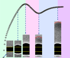
In this subsection, we present how the plume formation process is correlated to the development of the thermal boundary layer (TBL). Figure 4(a) shows four snapshots of shadowgraph images near the top surface of the heat source (indicated by the yellow dashed line). The measurement was made at  $Pr = 904.7$ and $Ra_{f} = 6.5 \times 10^6$ with continuous heating, so the generated thermal structure was in the starting stage of a plume, i.e. a starting plume. According to the working principle of shadowgraph technique, the TBL is displayed as a dark strip in these images, and the location with the strongest temperature gradient is the edge of the TBL (indicated by the yellow dots). Therefore, we can determine the thickness $\delta$ of the TBL by the vertical distance between the yellow line and the yellow dot. Note that the absolute value of $\delta$ is affected by the inevitable optical distortion in the shadowgraph measurements, so we just examine its change with time here.

Figure 4. (a) Shadowgraph images at four typical moments during the formation of a starting plume at  $Pr = 904.7$ and $Ra_{f} = 6.5 \times 10^6$. The complete process is shown in the supplementary movie available at https://doi.org/10.1017/jfm.2024.266. The pink dashed line highlights the position of the emitted plume. The yellow dashed line and dot represent the top surface of the resistor and the edge of the TBL, respectively, and their vertical distance is used to characterize the thickness $\delta$ of the TBL. (b) Plot of $\delta$ as a function of time after the heating power was turned on, from which four distinct stages separated by three characteristic times can be determined. (c) The three characteristic times as functions of $Ra_f$ at $Pr = 904.7$. Here, all the characteristic times have been normalized by the diffusive time $\tau _{0}=r_{0}^{2} / \kappa$ defined in § 2.1. The solid lines are power-law fits to each data set: $t_{emit}/\tau _{0}\sim Ra_f^{-0.31\pm 0.01},\ t_{recover}/\tau _{0}\sim Ra_f^{-0.52\pm 0.01}$ and $t_{static}/\tau _{0}\sim Ra_f^{-0.56\pm 0.04}$.
The  $\delta$ thus determined as a function of time is plotted in figure 4(b). It is seen that the evolution of $\delta$ can be divided into four stages: the growth stage, the emission stage, the recover stage and the quasi-static stage. Specifically, after the heating power is turned on at $t_{start}$, heat is conducted into the fluid and the TBL begins to build up. During the growth stage, the TBL grows in its thickness $\delta$, but remains stable. When $\delta$ reaches a critical value at $t = t_{emit}$, a plume starts to emit due to the instability of the TBL. Because some hot fluid parcels inside the TBL are taken away by the plume, the TBL shrinks, and its thickness $\delta$ decreases during the emission stage. As time goes by, the head of the plume becomes completely detached from the TBL at $t = t_{recover}$ and its tail appears, indicating the formation of a well-defined starting plume. At this critical moment, $\delta$ reaches a local minimum, then the TBL gets into the recover stage. During the recover stage, the TBL grows again gradually thanks to the continuous heating supplied from the heat source, and eventually becomes quasi-static at $t = t_{static}$. In the quasi-static stage, because all the heat supplied is taken away by the convection flow, the TBL becomes stable again and its thickness remains unchanged. It is interesting to note that similar evolution of the TBL thickness (growth–drop–stationary) was observed in some numerical studies of buoyancy-driven flows on a heated horizontal plate (Jiang, Nie & Xu Reference Jiang, Nie and Xu2019a,Reference Jiang, Nie and Xub; Jiang et al. Reference Jiang, Nie, Zhao, Carmeliet and Xu2021). However, these studies did not observe the recover stage as in the present experimental study. Further investigations combined with experiments and simulations are required to find the reason for this difference.
The complete process described above can be found in the supplementary movie, which clearly shows how the plume formation is correlated to the development of the TBL. During this process, three characteristic times are identified, and their  $Ra_f$ dependencies are plotted in figure 4(c). It is seen that $t_{emit} / \tau _{0}$, $t_{recover} / \tau _{0}$ and $t_{static} / \tau _{0}$ exhibit distinct $Ra_f$-dependent scaling exponents, being $-0.31$, $-0.52$ and $-0.56$, respectively. The scaling of $t_{recover}/ \tau _{0}$ recalls the study by Moses et al. (Reference Moses, Zocchi and Libchaberii1993), who predicted that the build-up time for starting plumes follows a relation $t_{build\text {-}up} / \tau _{0} \sim Ra_{f}^{-0.5}\,Pr^{0.5}$.
To compare our results with this theoretical prediction, we plot different characteristic times for all the  $Pr$ in figure 5. It is seen that $t_{recover}/\tau _{0}$ obeys a scaling relation $Ra_{f}^{-0.48}\,Pr^{0.48}$ for the present parameters explored, which is in good agreement with the theoretical prediction mentioned above. In terms of magnitude, $t_{recover}$ measured directly in the present study is very close to the experimental values of $t_{build\text {-}up}$ reported by Moses et al. (Reference Moses, Zocchi and Libchaberii1993). However, Moses et al. (Reference Moses, Zocchi and Libchaberii1993) did not measure $t_{build\text {-}up}$ directly. Instead, they assumed that the starting plume was originated from a ‘virtual point source $y_{virt}$’ at $t = 0$, and the plume's ascent height could be described by a function $y = V_{starting}(t-t_{build\text {-}up})$, where $V_{starting}$ is the rising velocity of the starting plume at the steady state. Then $t_{build\text {-}up}$ can be evaluated to be $t_{build\text {-}up} = -y_{virt}/V_{starting}$. Although the result yielded from this estimation ( $t_{build\text {-}up}/\tau _{0} \sim Ra_{f}^{-0.46}\,Pr^{0.46}$) is consistent with their theory, the obtained $t_{build\text {-}up}$ is physically ambiguous, and the data plotted in figure 5 are relatively scattered. This is in contrast to $t_{recover}$ in the present study, which can be determined precisely thanks to its clear physical meaning as revealed by figure 4.

Figure 5. Different normalized characteristic times as functions of  $Ra_{f}^{-0.5}\,Pr^{0.5}$. The solid symbols are the build-up times for starting plumes measured indirectly by Moses et al. (Reference Moses, Zocchi and Libchaberii1993). The solid lines are the best power-law fits to each data group.
The physical meaning of  $t_{emit}$ is also revealed unambiguously by figure 4. This data group can be fitted by a power law $t_{emit}/\tau _0 \sim Ra_{f}^{-0.41}\,Pr^{0.41}$. To understand this scaling relation, we note that at the moment of plume emission, the time duration for heating power being supplied to the fluid (i.e. the heating time $t_{heat}$) is equal to $t_{emit}$. Therefore, we can substitute $t_{emit}$ into the definition of Rayleigh number $Ra = t_{heat}\,Ra_{f}/\tau _0\,Pr$ (see the last paragraph in § 2.1) to quantify the total buoyancy supplied to the fluid at this moment. Specifically, we can substitute $Ra_{f}/Pr = Ra\,\tau _0/ t_{emit}$ into the scaling relation $t_{emit}/\tau _0 \sim Ra_{f}^{-0.41}\,Pr^{0.41}$, which leads immediately to $t_{emit}/\tau _0 \sim Ra^{-0.69}$. This result is in good agreement with a phenomenological model developed by Howard (Reference Howard1966), who predicted that the onset time for the instability of the TBL scales with $Ra$ as $Ra^{-2/3}$. Similar scaling exponents have been reported in some previous experiments (Vest & Lawson Reference Vest and Lawson1972; Davaille & Vatteville Reference Davaille and Vatteville2005). However, these studies determined the onset time by watching the convection patterns instead of measuring the TBL directly, so the correlation between the plume emission and the TBL instability has not been revealed explicitly as in the present study.
Compared to  $t_{recover}$ and $t_{emit}$, the data group $t_{static}$ is relatively scattered and does not collapse well for different $Pr$. Nevertheless, a simple power-law fit to this data group yields a relation $t_{static}/\tau _{0} \sim Ra_{f}^{-0.38}\,Pr^{0.38}$. If a least squares method is used to determine the best $Ra_f$ and $Pr$ scaling exponents, then we obtain $t_{static}/\tau _{0} \sim Ra_{f}^{-0.49}\,Pr^{0.33}$ (not shown here). The latter scaling relation might be more reasonable, but we do not have a theory for it at this stage. According to figure 4(b), $t_{static}$ is the moment when the TBL changes from the recover stage to the quasi-static stage. Thus it is more meaningful to check the time duration for the TBL to recover, i.e. $t_{static}-t_{recover}$. However, no clear $Ra_{f}$– $Pr$ dependence is found for this time duration either, so we do not present the data here. It is noteworthy that a similar recover process exists in turbulent convection experiments due to the so-called finite conductivity effect, which could influence the plume emission and even the heat transport properties (Brown et al. Reference Brown, Nikolaenko, Funfschilling and Ahlers2005; Sun & Xia Reference Sun and Xia2007). It would be interesting to quantify this process in turbulent convection experiments and compare with the present results in future studies.
To further examine the correlation between the plume formation and the TBL development, we plot in figure 6 the plume's rising velocity and the corresponding acceleration together with the TBL thickness. Because similar behaviours have been observed for different  $Pr$, the data measured at $Pr = 904.7$ are taken as the example for discussion. Note that the acceleration plotted here is calculated by taking the time derivative of the rising velocity. A Gaussian convolution method was adopted to reduce the data noise (Mordant et al. Reference Mordant, Crawford and Bodenschatz2004), so there are no acceleration data at the very beginning of the time series. In addition, the plume has not formed before $t = t_{emit}$, so the velocity and acceleration before this moment are the data inside the TBL. It is seen in figure 6(a) that there is a time delay in the evolution curves between the plume and the TBL. Such a time delay is much clearer in figure 6(b), which seems to be a constant in units of $t_{recover}$. While the TBL thickness becomes unchanged after $t \simeq 1.5t_{recover}$, the rising velocity of the plume does not reach the steady state until $t \simeq 2.5t_{recover}$. The time delay can also be observed in the acceleration of the plume (see figures 6c,d). Noticeably, the normalized accelerations $A/A_{max}$ for different $Ra_f$ almost fall into a single curve once they are plotted against $t/t_{recover}$, just as for the normalized rising velocities $V/V_{max}$ shown in figure 6(b). These results not only provide further information about the correlation between the plume formation and the TBL development, but also suggest that $t_{recover}$ is a crucial time scale during the plume evolution process, which will be discussed further in the following subsections.

Figure 6. (a) Temporal evolution of the TBL thickness determined from shadowgraph (lines) and the plume's rising velocity obtained from PIV (symbols) for different  $Ra_f$ at $Pr = 904.7$. (b) The same data as in (a), but normalized by using the maximum TBL thickness, the maximum rising velocity and $t_{recover}$. Note that these quantities used for normalization have different values for different $Ra_f$. (c,d) The relation between the TBL thickness and the plume's acceleration is examined in a similar way as in (a,b).
3.2. Effects of heating time
In the previous subsection, we have shown that there exist four distinct stages during the plume formation process. In this subsection, we present a quantitative comparison of the properties of thermal structures emitted at different stages, i.e. generated by different heating times  $t_{heat}$. To examine the effects of $t_{heat}$ in a better way, $Ra_f$ was fixed at $Ra_f = 6.5 \times 10^6$. We first show the results measured at $Pr=904.7$. The three characteristic times for this $Pr$ at $Ra_f = 6.5 \times 10^6$ are $t_{emit} = 6.6$ s, $t_{recover} = 10.6$ s and $t_{static}= 16.3$ s, so $t_{heat}$ was varied from 3.0 to 16.3 s, corresponding to an $Ra$ ( $= t_{heat}\,Ra_{f}/\tau _0\,Pr$) number range $900 \leq Ra \leq 4900$.
Figure 7(a) plots the temporal evolution curves of the rising velocities of thermal structures generated by different  $t_{heat}$ (or equivalently different $Ra$). The data of the starting plume are plotted together for comparison. It is seen that the maximum rising velocities in these curves increase monotonically with increasing $t_{heat}$, and the upper limit is bounded by the case of the starting plume. Based on their variation trends, these curves can be divided into two groups. For thermal structures generated by $t_{heat} \geq t_{emit}$ ( $=6.6$ s), their rising velocities first increase quickly in a manner like the starting plume, and then decay slowly like a thermal after reaching the maximum value (demonstrated in § 3.3). Note that these thermal structures can be viewed as detached TBLs, so their almost-collapsed curves in the accelerating stage could be originated from the dynamics inherited from the unstable TBL, which is commonly believed in studies of Rayleigh–Bénard convection (Ahlers et al. Reference Ahlers, Grossmann and Lohse2009). However, for the cases with $t_{heat} < t_{emit}$, their rising velocities show a different trend in the accelerating stage. This is because these thermal structures are not emitted from the TBL due to instability. Rather, they are hot fluid parcels adjacent to the heat source, which go up after the heating power is turned off thanks to their own buoyancy. In this context, their generation process is similar to a sudden release of a hot fluid parcel in some experimental studies of thermals (see e.g. Griffiths Reference Griffiths1986).

Figure 7. (a,b) Temporal variations of (a) the rising velocity and (b) the corresponding acceleration of thermal structures generated by different heating times (or equivalently different  $Ra$) at $Pr = 904.7$ and $Ra_f=6.5\times 10^6$. (c,d) The dimensionless maximum velocity $V_{max}/u_{0}$ and the dimensionless maximum acceleration $A_{max}/a_{0}$ as functions of (c) $Ra$ and (d) the dimensionless heating time $t_{heat}/t_{recover}$. The corresponding values of the starting plume are indicated by the purple solid line (dimensionless maximum velocity) and the blue solid line (dimensionless maximum acceleration), respectively.
The acceleration plotted in figure 7(b) confirms that  $t_{emit}$ is the characteristic time that determines whether thermal structures generated by finite $t_{heat}$ will have similar evolution dynamics. It is seen clearly that the accelerations of thermal structures with $t_{heat} < t_{emit}$ are much weaker than in the cases with $t_{heat} \geq t_{emit}$, and exhibit an obvious different trend in the accelerating stage. For thermal structures with $t_{heat} \geq t_{emit}$, their acceleration curves largely follow the trend of the starting plume, except for the decay behaviour. To be specific, the acceleration of the starting plume decreases monotonically from the maximum value to a steady level close to zero. By contrast, the data for thermal structures with $t_{heat} \geq t_{emit}$ first decay to negative values that are well below zero, and then increase gradually to the level of the starting plume. A close look at figures 7(a,b) reveals that the moment when the acceleration drops to zero is the moment when the rising velocity reaches the maximum value. This phenomenon can be found for all the thermal structures generated by finite $t_{heat}$, though it is not that obvious for the cases with $t_{heat} < t_{emit}$. To understand this result, we note that thermal structures generated by finite $t_{heat}$ do not have an energy supply after the heating power is turned off, thus the viscous drag becomes significant in the decelerating stage and leads to negative accelerations. As the viscous drag is larger for larger rising velocity, one can see in figure 7(b) that the drop in acceleration is stronger for larger $t_{heat}$.
To examine quantitatively how  $t_{heat}$ affects the properties of thermal structures, we take the maximum velocity and the maximum acceleration as the characteristic quantities, and plot their dimensionless values in figures 7(c,d). It is seen that the maximum velocity increases with $Ra$ (or the dimensionless heating time $t_{heat}/t_{recover}$) and approaches the value of the starting plume gradually. Based on the variation trend of $V_{max}/u_0$ in figure 7(d), the maximum velocity of thermal structures generated by finite $t_{heat}$ will be equal to the value of the starting plume when $t_{heat} \simeq 2.5t_{recover}$. This time scale is consistent with the data shown in figure 6(b), where one can see that the rising velocity of the thermal structure reaches the steady state at approximately $2.5t_{recover}$.
The maximum acceleration  $A_{max}/a_{0}$ also increases with $t_{heat}/t_{recover}$ and reaches the value of the starting plume at $t_{heat} \simeq t_{recover}$. For larger $t_{heat}$, $A_{max}/a_{0}$ remains unchanged. This behaviour could be understood as follow. Although the thermal structure begins to emit at $t_{emit}$, the emission process does not complete until $t_{recover}$. During the emission process, the thermal structure can gain buoyancy energy from the TBL directly, so its acceleration can increase to a larger value if the heating power supply is continued. At the moment of $t_{recover}$, the thermal structure is fully detached from the TBL, and its buoyancy energy is fed by the long tail after then, just as in the case of the starting plume. Therefore, the maximum acceleration reaches the value of the starting plume at $t_{heat} = t_{recover}$. And because the rising velocity does not reach the maximum value until the acceleration becomes zero, the maximum velocity approaches the value of the starting plume at a larger value of $t_{heat}/t_{recover}$.
These asymptotic behaviours can be observed for all the  $Pr$ explored in the present study. As shown in figures 8(c,d), while $V_{max}/u_0$ for different $Pr$ seem to approach the upper limit values at different $t_{heat}/t_{recover}$, $A_{max}/a_0$ for different $Pr$ reach different plateaus roughly at the same condition ( $t_{heat}/t_{recover} \simeq 1$). Noticeably, if $A_{max}/a_0$ is plotted against $Ra$, then the values almost fall onto a single curve before reaching the plateaus (see figure 8b). A more remarkable finding comes from the data shown in figure 8(a). It is seen that $V_{max}/u_0$ for different $Pr$ collapse well over the present $Ra$ number range. However, these data do not follow a simple scaling law. Instead, they experience a transition from $V_{max}/u_0 \sim Ra$ to $V_{max}/u_0 \sim (Ra\ln Ra)^{0.5}$ at $Ra \simeq 6000$. To understand this scaling transition, we note that thermal structures generated by finite $t_{heat}$ contain finite amounts of buoyancy and thus can be viewed as thermals. However, according to the data shown in figure 6(b), if $t_{heat}$ is larger than 2.5 $t_{recover}$, then these thermal structures will get into the quasi-static stage and go up with constant rising velocities like plumes. Since the maximum heating times examined in figure 8 are all smaller than 2.5 $t_{recover}$, these data can be understood by the behaviours of thermals. For the scaling relation below $Ra \simeq 6000$, it is consistent with previous studies of thermals at low $Ra$ (Morton Reference Morton1960; Shlien & Thompson Reference Shlien and Thompson1975); for that above $Ra \simeq 6000$, it is in excellent agreement with the model prediction and the numerical results by Whittaker & Lister (Reference Whittaker and Lister2008). Interestingly, if a simple power law is attempted to fit all the data in figure 8(a), then the scaling relation turns out to be $V_{max}/u_0 \sim Ra^{0.78}$ (not shown in the figure for clarity), which is in line with the experimental finding and the model prediction ( $V_{max}/u_0 \sim Ra^{0.75}$) by Griffiths (Reference Griffiths1986). Therefore, the present data provide not only experimental evidence for the existence of the $(Ra\ln Ra)^{0.5}$ scaling for thermals at large $Ra$, but also a unifying understanding of the seemingly inconsistent scaling relations observed in previous studies (Morton Reference Morton1960; Shlien & Thompson Reference Shlien and Thompson1975; Griffiths Reference Griffiths1986; Whittaker & Lister Reference Whittaker and Lister2008).

Figure 8. (a,c) The dimensionless maximum velocity  $V_{max}/u_0$ and (b,d) the dimensionless maximum acceleration $A_{max}/a_0$ as functions of (a,b) $Ra$, and (c,d) the dimensionless heating time $t_{heat}/t_{recover}$ for different $Pr$ at $Ra_f=6.5\times 10^6$. The black and blue solid lines in (a) are two different power laws, as labelled.
3.3. Characteristics of thermal structures generated by  $t_{heat} = t_{recover}$

Based on the results presented in §§ 3.1 and 3.2, we have found that  $t_{recover}$ is a crucial time scale during the formation and evolution of thermal structures. In particular, it is the critical moment when the thermal structure is fully detached from the TBL and the corresponding maximum acceleration reaches an upper limit. Since thermal structures generated by different heating times $t_{heat}$ have similar evolution dynamics once $t_{heat} \ge t_{emit}$, we can take the case with $t_{heat} = t_{recover}$ as an example to examine their evolution dynamics in detail, which is the focus of this subsection. Again, we will present first the results measured at $Pr=904.7$ and then the data for different $Pr$.
$Pr$.
Figure 9 shows the evolution curves of the rising velocities of thermal structures generated by  $t_{heat}=t_{recover}$ for different $Ra_f$ at $Pr = 904.7$. The data have been plotted in different ways to show every detailed feature during the evolution. It is seen in figure 9(a) that the curves for different $Ra_f$ have a similar shape, where the higher $Ra_f$ case has a larger maximum rising velocity $V_{max}$ that occurs at a shorter time. If we take $V_{max}$ and $t_{recover}$ as the referenced units, then the normalized velocity $V/V_{max}$ as a function of $t/t_{recover}$ for different $Ra_f$ collapses onto a universal curve when $t / t_{recover} \le 2.5$ (see figure 9b). The three characteristic times for the $Ra_f=6.5\times 10^6$ case are also highlighted in figure 9(b), indicating that the evolution trends are different before and after $t_{emit}$. However, we note that the data collapse could not be achieved by using $t_{emit}$ as the referenced time. Moreover, the universal behaviour applies only to the data within $t / t_{recover} \simeq 2.5$, after which the data for different $Ra_f$ become diverged (see the inset of figure 9b).

Figure 9. (a) Temporal variations of the rising velocities of thermal structures generated by  $t_{heat}=t_{recover}$ for different $Ra_f$ at $Pr = 904.7$. (b) The same results as in (a), but normalized by the maximum rising velocity $V_{max}$ and the characteristic time $t_{recover}$ for each $Ra_f$. The inset shows that the data for different $Ra_f$ begin to diverge when $t / t_{recover} \gtrsim 2.5$. (c) A similar plot as in (b), but the data are normalized by the diffusive velocity $u_{0}$ ( $= r_0/\tau _0$). The solid curves are the best fits to each data set for $t / t_{recover} \gtrsim 2.5$. (d) The same data as in (c), with the fitting curves extended to the stagnant time $t_{stag}$, at which the rising velocity becomes zero and the thermal structure reaches the maximum ascent height $H_{max}$. Inset: the dimensionless stagnant time $t_{stag}/t_{recover}$ and the dimensionless maximum ascent height $H_{max}/r_0$ as functions of $Ra_f$. The solid lines are power-law fits to each data set: $t_{stag}/t_{recover} \sim Ra_f^{0.50}$ and $H_{max}/r_{0} \sim Ra_f^{0.31}$. See text for detailed explanations.
For the time period  $t / t_{recover} > 2.5$, the thermal structures have got into the decelerating stage without heat supply and are dominant by the viscous drag. Therefore, we take the diffusion velocity $u_0$ ( $=r_0/\tau _0$) as the referenced velocity, and plot $V/u_{0}$ as a function of $t/t_{recover}$ in figure 9(c). Although this dimensionless form does not yield a data collapse, the data in the decelerating stage ( $t / t_{recover} > 2.5$) for different $Ra_f$ exhibit a similar shape and can be fitted by a relation $V/u_{0} \sim (t/t_{recover}-1)^{-0.5} - V_{virt}$, which is proposed to describe the evolution behaviour of thermals (Morton Reference Morton1960; Griffiths Reference Griffiths1986). Here, $V_{virt}$ is known as the virtual velocity, as the rising velocity should approach zero as the time goes to infinity.
Actually, thermal structure generated by a finite heating time should have a finite lifetime. With this in mind, we define the stagnant time  $t_{stag}$ when the rising velocity decays to zero. At this moment, the thermal structure becomes stagnant and reaches the maximum ascent height $H_{max}$. Figure 9(d) illustrates how this characteristic time is determined from the decay curves of the rising velocity. The dimensionless stagnant time $t_{stag} / t_{recover}$ thus determined is found to scale with $Ra_f$ as $t_{stag}/t_{recover} \sim Ra_f^{0.50}$ (see the inset of figure 9d). As $t_{recover}/\tau _0\sim Ra_f^{-0.48}$, we can infer that $t_{stag}$ is almost independent of $Ra_f$, implying that this time scale is determined by a diffusion process. The corresponding maximum ascent height $H_{max}$ can also be obtained by integrating the rising velocity to the moment $t = t_{stag}$. The data thus obtained are plotted in the inset of figure 9(d), and they follow a scaling relation as $H_{max}/r_{0} \sim Ra_f^{0.31}$. This scaling exponent coincides with the predicted scaling $1/3$ by a theoretical model of turbulent atmospheric plumes (Stothers Reference Stothers1989), despite the present scenario being laminar thermal structures in a homogeneous stationary fluid layer.
The analysis above suggests three characteristic quantities for further examination with different  $Pr$: the maximum rising velocity $V_{max}$ during the evolution, the stagnant time $t_{stag}$, and the maximum ascent height $H_{max}$. We first check the $Pr$ dependencies of $t_{stag}$ and $H_{max}$. Figure 10(a) shows the dimensionless stagnant time $t_{stag}/t_{recover}$ as a function of $Pr$ for different $Ra_f$. It is seen that these data sets can all be described by power-law fittings, with the scaling exponents ranging from 0.06 to 0.12. Because the $Ra_f$-dependent scalings of $t_{stag}/t_{recover}$ are close to 0.50 for all $Pr$ (not shown here), we compensate the data in figure 10(a) by ${Ra_f}^{0.50}$ to collapse them into a single line (see figure 10b); then a power-law fit to all the data yields a $Pr$-dependent scaling 0.08, i.e. $t_{stag}/t_{recover}\sim {Ra_f}^{0.50}\,Pr^{0.08}$, or equivalently, $t_{stag}/\tau _0\sim {Ra_f}^{0.02}\,Pr^{0.56}$. Through a similar procedure, we obtain the $Ra_f$– $Pr$ dependence of the maximum ascent height as $H_{max}/r_0\sim {Ra_f}^{1/3}\,Pr^{0.16}$ (see figures 10c,d). To the best of our knowledge, no theory has studied the stagnant time before. However, the maximum ascent height has received much of interest, as it is relevant to a range of natural phenomena, such as cloud rise and volcanic eruption (Wilson et al. Reference Wilson, Sparks, Huang and Watkins1978; Sparks Reference Sparks1986; Stothers Reference Stothers1989; Hansen et al. Reference Hansen, Esposito, Stewart, Colwell, Hendrix, Pryor and West2006; Glaze et al. Reference Glaze, Self, Schmidt and Hunter2017). The scaling relations obtained here, especially the less-explored $Pr$ dependencies, might be helpful to understand the relevant processes in nature.

Figure 10. (a) The dimensionless stagnant time  $t_{stag}/t_{recover}$ as a function of $Pr$ for different $Ra_f$. The solid lines are power-law fits to each data set. (b) Plots of $t_{stag}/t_{recover}$ compensated by ${Ra_f}^{0.50}$ as a function of $Pr$. The solid line is the best power-law fit to all the data points: $t_{stag}/t_{recover}\sim {Ra_f}^{0.50}\,Pr^{0.08}$. (c) The dimensionless maximum ascent height $H_{max}/r_0$ as a function of $Pr$ for different $Ra_f$. The solid lines are power-law fits to each data set. (d) Plots of $H_{max}/r_0$ compensated by ${Ra_f}^{1/3}$ as a function of $Pr$. The solid line is the best power-law fit to all the data points: $H_{max}/r_0\sim {Ra_f}^{1/3}\,Pr^{0.16}$.
Finally, we examine the maximum rising velocity  $V_{max}$ of thermal structures generated by $t_{heat} = t_{recover}$ in figure 11. Also plotted in the figure are the results of starting plumes obtained in two previous studies (Moses et al. Reference Moses, Zocchi and Libchaberii1993; Kaminski & Jaupart Reference Kaminski and Jaupart2003) as well as in the present work. Note that for starting plumes, their maximum rising velocities are the values at the steady state (see figure 6b). According to Moses et al. (Reference Moses, Zocchi and Libchaberii1993), the dimensionless maximum rising velocities of starting plumes $V_{max}/u_0$ obey a scaling law as $V_{max}/u_0 \sim Ra_{f}^{0.5}\,Pr^{-0.5}$. This scaling law is supported by their experimental data obtained by the shadowgraph technique, which can be described by a relation $Ra_{f}^{0.46}\,Pr^{-0.46}$ approximately. However, by conducting new measurements with the differential interferometry technique, Kaminski & Jaupart (Reference Kaminski and Jaupart2003) found that starting plumes can rise much faster than the results reported by Moses et al. (Reference Moses, Zocchi and Libchaberii1993), though the scaling exponents in these two studies are basically consistent (see black and blue lines in figure 11). As discussed by Kaminski & Jaupart (Reference Kaminski and Jaupart2003), the discrepancy in magnitude could be due to some experimental artefacts, such as sidewall effects, free-surface effects and thermal leakage. Our present results obtained by PIV measurements over a different $Pr$ range are in good agreement with the data by Kaminski & Jaupart (Reference Kaminski and Jaupart2003), including both the scaling exponent and the magnitude. This good agreement provides support for the study by Kaminski & Jaupart (Reference Kaminski and Jaupart2003) on the one hand, and verifies the reliability of the present experiments on the other.

Figure 11. The dimensionless maximum rising velocities of thermal structures as functions of  $Ra_{f}^{0.5}\,Pr^{-0.5}$ for different parameter settings. The results obtained in previous studies by Moses et al. (Reference Moses, Zocchi and Libchaberii1993) and Kaminski & Jaupart (Reference Kaminski and Jaupart2003) are plotted for comparison. See text for a detailed explanation.
In contrast to the behaviour of starting plumes,  $V_{max}/u_0$ of thermal structures generated by $t_{heat} = t_{recover}$ exhibit a different $Ra_f$– $Pr$ dependence. A simple power-law fit to these data yields a scaling relation $V_{max}/u_0 \sim Ra_{f}^{0.37}\,Pr^{-0.37}$. If a least squares method is used to fit this data group, then the $Ra_f$ and $Pr$ scaling exponents change little, being 0.41 and $-$0.37, respectively (not shown here). To understand this scaling relation, we define a Reynolds number $Re$ as $Re = V_{max}r_0/\nu$ based on this data group. By using the definitions of $\tau _0$, $u_0$, $Ra$ and $Pr$, namely $\tau _0 = r_0^2 / \kappa$, $u_0 = r_0/\tau _0 = r_0\,Pr/\nu$ and $Ra = t_{heat}\,Ra_{f}/\tau _0\,Pr$, and noticing that $t_{heat} = t_{recover}$ for this data group where $t_{recover}/\tau _0\sim Ra_f^{-0.48}\,Pr^{0.48}$, we obtain $Re \sim Ra^{0.71}\,Pr^{-1}$. This result recalls the scaling relation $Re \sim Ra^{2/3}\,Pr^{-1}$ predicted by a theoretical model for large- $Pr$ natural thermal convection (Shishkina et al. Reference Shishkina, Emran, Grossmann and Lohse2017). It is also worth mentioning that in previous studies of turbulent Rayleigh–Bénard convection with large $Pr$ (Lam et al. Reference Lam, Shang, Zhou and Xia2002; Silano, Sreenivasan & Verzicco Reference Silano, Sreenivasan and Verzicco2010; Li et al. Reference Li, He, Tian, Hao and Huang2021a), the observed $Re$–
$Re$– $Ra$ scaling exponents (ranging from 0.65 to 0.74) are compatible with the present value. However, it should be stressed that the convection systems examined in these studies (Lam et al. Reference Lam, Shang, Zhou and Xia2002; Silano et al. Reference Silano, Sreenivasan and Verzicco2010; Shishkina et al. Reference Shishkina, Emran, Grossmann and Lohse2017; Li et al. Reference Li, He, Tian, Hao and Huang2021a) are turbulent flows, while the present study addresses laminar thermal structures. Thus it is interesting to see the good match of the scaling exponents between different studies. One possible explanation is that large- $Pr$ thermal convection is dominant by slender thermal structures, and no large-scale mean flow exists in the system (Li et al. Reference Li, He, Tian, Hao and Huang2021a). As a result, the flow velocity first increases with growing distance away from the boundary, and then decays slowly to zero after reaching the maximum, which is similar to the present situation. These similar flow features might be the origin of the similar scaling relations observed in different studies.
4. Conclusion
In summary, we have conducted a series of experiments to investigate the formation and evolution of laminar thermal structures generated by a small heat source. The experiments were performed over the flux Rayleigh number  $Ra_f$ range $2.1\times 10^6 \leq Ra_f \leq 3.6\times 10^{7}$ and the Prandtl number $Pr$ range of $28.6 \leq Pr \leq 904.7$. In order to examine the properties of thermal structures generated by finite heating time $t_{heat}$, $t_{heat}$ was also varied in some experiments, with $Ra_f$ fixed at $6.5\times 10^{6}$, resulting in a Rayleigh number $Ra$ range $900 \leq Ra \leq 4\times 10^{4}$. Based on the experimental data with different parameter settings ( $\sim$110 cases in total), we came to the main findings below.
First, through examining the correlation between the plume formation and the thermal boundary layer (TBL) development, three characteristic times were observed during the plume formation process, namely  $t_{emit}$, $t_{recover}$ and $t_{static}$. Specifically, when the plume starts to emit due to the TBL instability, the TBL thickness reaches a maximum that gives rise to the determination of $t_{emit}$. As the plume emits, the TBL thickness decreases and reaches a local minimum when the plume's head is completely detached from the TBL. This critical moment $t_{recover}$ turns out to be the build-up time for starting plumes as evaluated (without direct measurements) in the literature (Moses et al. Reference Moses, Zocchi and Libchaberii1993). The $Ra_f$– $Pr$ dependencies of $t_{emit}$ and $t_{recover}$ are found to be $Ra_f^{-0.41}\,Pr^{0.41}$ and $Ra_f^{-0.48}\,Pr^{0.48}$, respectively, which are in good agreement with the theories (Howard Reference Howard1966; Moses et al. Reference Moses, Zocchi and Libchaberii1993). As for $t_{static}$, it is the moment when the TBL gets into the steady state and obeys a scaling relation $Ra_f^{-0.49}\,Pr^{0.33}$. The plume reaches the steady state with a time delay, which is a constant in units of $t_{recover}$.
Based on these characteristic times, the effects of heating time  $t_{heat}$ on thermal structures were investigated. It is found that once $t_{heat} \gtrsim t_{emit}$, thermal structures generated by different $t_{heat}$ will have similar evolution dynamics, with the accelerating stage like starting plumes, and the decay stage like thermals. In particular, by using the diffusion velocity as the normalized unit, the dimensionless maximum rising velocities of these thermal structures exhibit a universal behaviour, which experiences a crossover in the scaling relation from $Ra$ to $(Ra\ln Ra)^{0.5}$ as $Ra$ increases (by increasing $t_{heat}$). This finding not only provides experimental evidence for the theoretically predicted scaling $(Ra\ln Ra)^{0.5}$ for thermals at large- $Ra$ (Whittaker & Lister Reference Whittaker and Lister2008), but also explains the inconsistent results reported in previous studies of thermals (Morton Reference Morton1960; Shlien & Thompson Reference Shlien and Thompson1975; Griffiths Reference Griffiths1986; Whittaker & Lister Reference Whittaker and Lister2008; Peng & Lister Reference Peng and Lister2014).
It is further found that the maximum accelerations of thermal structures generated by finite  $t_{heat}$ have a saturated value bounded by the case of starting plumes. This saturation occurs at $t_{heat} \simeq t_{recover}$, implying that $t_{recover}$ is a crucial time scale during the evolution process of these thermal structures. Therefore, the characteristics of thermal structures generated by $t_{heat} = t_{recover}$ were examined in detail. The most interesting findings about these thermal structures are their maximum ascent height $H_{max}$ and maximum rising velocity $V_{max}$, which follow the scaling relations $Ra_f^{1/3}\,Pr^{0.16}$ and $Ra_f^{0.37}\,Pr^{-0.37}$, respectively. It is not clear at this stage how $t_{heat}$ would affect these two scaling relations. Further investigations should be conducted to address this issue quantitatively.
Before ending this paper, we would like to highlight one issue that is relevant to one of the motivations of the present study. As we discussed in the Introduction, the emission of thermal structures in turbulent Rayleigh–Bénard convection is a co-action of the TBL instability and the perturbation from turbulent flow. As a result, the thermal structures emit at different stages from the TBL and thus supply different amounts of buoyancy energy to drive the convection flow. It is not clear whether these thermal structures would exhibit different behaviours and contribute to the anomalous scaling observed in turbulent Rayleigh–Bénard convection (Brown, Funfschilling & Ahlers Reference Brown, Funfschilling and Ahlers2007; Ching Reference Ching2007; Li et al. Reference Li, Huang, Ni and Xia2021b). In the present study, we have shown that once thermal structures emit at a time scale larger than the onset time that determines the TBL instability, they will have similar evolution dynamics, despite the magnitudes of their rising velocity and acceleration being different. However, this result was obtained in a stationary fluid layer without a background flow. It would be interesting to check the present finding by imposing a mean flow above the heat source, which is beyond the scope of the present study but an exciting issue to explore in the future.
Supplementary movie
A supplementary movie is available at https://doi.org/10.1017/jfm.2024.266.
Acknowledgements
We thank L. Sun for participating in the early stage of this project.
Funding
This work was supported by the National Natural Science Foundation of China (NSFC grant nos 12272162, 11961160719 and 11702128) and the Department of Science and Technology of Guangdong Province (grant no. 2023B1212060001). P.W. was supported in part by an NSFC grant (no. 11872281).
Declaration of interests
The authors report no conflict of interest.


