


1. Introduction
Debris flows have attracted the attention of scientists due to the catastrophic nature of the hazards that they pose (Iverson Reference Iverson1997; McSaveney, Beetham & Leonard Reference McSaveney, Beetham and Leonard2005). A devastating example is that of the 8 August 2010 debris flow in the northwestern Chinese province of Gansu, which caused more than 1000 deaths in the county of Zhouqu (Ren Reference Ren2014). Two other prominent recent examples are when heavy rainfall triggered 107 debris flows in Hiroshima city in southwest Japan on 20 August 2014 (Wang et al. Reference Wang, Wu, Yang, Tanida and Kamei2015), which caused 44 injuries and 74 deaths, as well as a torrent of rock, ice, sediment and water in Uttarakhand in northern India (Sati Reference Sati2022), which killed hundreds of people and devastated two hydropower stations on 7 February 2021. In recent years, debris flow frequency has increased, due to the increased intensity of rainfall events (Ballantyne Reference Ballantyne2002), glacial melt water, severe forest fires (Kean et al. Reference Kean, Staley, Lancaster, Rengers, Swanson, Coe, Hernandez, Sigman, Allstadt and Lindsay2019) and the melting of permafrost (Higman et al. Reference Higman2018), which has made previously stable slopes unstable. This provides strong motivation for the study of the dynamics of debris flows, with the goal of minimising damage to people and infrastructure.
One of the most destructive features of debris flows is the initial deep surge, which is drier than the main body and is often rich in boulders and larger particles. A typical example is shown in figure 1(a) and the supplementary online video (movie 1) available at https://doi.org/10.1017/jfm.2022.400, where a very rapidly moving debris front narrowly misses a group of hikers in Aconcagua Park in Argentina. After the initial bouldery surge, the flow slowly wanes in height at the same time as the largest surface grains decrease in size and the flow becomes increasingly watery (figure 1b). A series of secondary drier boulder-rich surges that transition to watery tails then propagate down the channel at 40, 71 and 160 seconds. These poorly understood phenomena are often observed in the field (Costa & Williams Reference Costa and Williams1984; Pierson Reference Pierson1986; Kean et al. Reference Kean, McCoy, Tucker, Staley and Coe2013) and in large-scale debris-flow experiments (Iverson et al. Reference Iverson, Logan, Lahusen and Berti2010; Johnson et al. Reference Johnson, Kokelaar, Iverson, Logan, LaHusen and Gray2012). Closely related flow features can also develop in suspensions (Murisic et al. Reference Murisic, Pausader, Peschka and Bertozzi2013), snow avalanches (Gray & Hutter Reference Gray and Hutter1997) and pyroclastic flows (Mangeney et al. Reference Mangeney, Bouchut, Thomas, Vilotte and Bristeau2007), as well as in small-scale wet and dry analogue experiments (Félix & Thomas Reference Félix and Thomas2004; Woodhouse et al. Reference Woodhouse, Thornton, Johnson, Kokelaar and Gray2012; Kokelaar et al. Reference Kokelaar, Graham, Gray and Vallance2014; de Haas et al. Reference de Haas, Braat, Leuven, Lokhorst and Kleinhans2015; Scheidl, McArdell & Rickenmann Reference Scheidl, McArdell and Rickenmann2015; Baker, Johnson & Gray Reference Baker, Johnson and Gray2016a; Lanzoni, Gregoretti & Stancanelli Reference Lanzoni, Gregoretti and Stancanelli2017).

Figure 1. Debris flow on 27 January 2015 in Aconcagua Park, Mendoza, Argentina (copyright Julian Insarralde via ViralHog). (a) A large amplitude dry bouldery flow front propagates down a channel at approximately 6 m s $^{-1}$, forcing hikers to scramble to safety. (b) Eighteen seconds later, the height of the flow has reduced, there are no surface boulders and the flow is much more watery. Movie 1 in the online supplementary material shows that the main pulse is followed by a series of bouldery surges, 40, 71 and 160 seconds after the arrival of the main front, which are interspersed by lower amplitude watery sections.
Since the water typically experiences less friction than the grains, many existing debris flow models predict that water moves to the front of the flow (George & Iverson Reference George and Iverson2011; Pudasaini Reference Pudasaini2012). As a result, the formation of dry snouts is often attributed to particle-size segregation (see Vallance & Savage Reference Vallance and Savage2000; Gray & Ancey Reference Gray and Ancey2009; Iverson et al. Reference Iverson, Logan, Lahusen and Berti2010; Johnson et al. Reference Johnson, Kokelaar, Iverson, Logan, LaHusen and Gray2012; George & Iverson Reference George and Iverson2014; Baker et al. Reference Baker, Johnson and Gray2016a; Liu et al. Reference Liu, He, Chen, Yan and Deng2020) and the two ideas have become conflated. Certainly, the vertical ordering provided by particle-size segregation (i.e. that during shear, large particles tend to rise above finer grains) combined with velocity shear leads to differential longitudinal transport of the large and small particles and the formation of a bouldery snout (Gray & Ancey Reference Gray and Ancey2009; Gray & Kokelaar Reference Gray and Kokelaar2010; Johnson et al. Reference Johnson, Kokelaar, Iverson, Logan, LaHusen and Gray2012; Gray Reference Gray2018), but there is no clear reason why the snout should be dry.
The moving bed flume experiments of Davies (Reference Davies1988, Reference Davies1990), with monodisperse-particle–fluid mixtures, show that dry fronts can develop even in the absence of particle segregation. Similar dry fronts also develop in monodisperse-particle–fluid mixtures in rotating drums (Leonardi et al. Reference Leonardi, Cabrera, Wittel, Kaitna, Mendoza, Wu and Herrmann2015) and on chutes (Taylor-Noonan Reference Taylor-Noonan2020). This implies that the dry snouts do not require particle-size segregation, which motivates the development, in this paper, of a new depth-averaged model for monodisperse-particle–fluid mixtures that can account for their formation. As with particle-size segregation, vertical structure and velocity shear will play a key role in its derivation.
Despite its importance, velocity shear is completely neglected in most debris-flow models which assume plug flow through their depth (Iverson Reference Iverson1997; Iverson & Denlinger Reference Iverson and Denlinger2001; Pitman & Le Reference Pitman and Le2005; Pailha & Pouliquen Reference Pailha and Pouliquen2008; Pudasaini Reference Pudasaini2012; Iverson & George Reference Iverson and George2014; Bouchut et al. Reference Bouchut, Fernadez-Nieto, Mangeney and Narbona-Reina2016). Johnson et al.'s (Reference Johnson, Kokelaar, Iverson, Logan, LaHusen and Gray2012) large-scale debris-flow experiments at the United States Geological Survey (USGS) flume show that there is in fact strong internal velocity shear through the flow depth. The flow spread out strongly along the main body of the chute, and entered a locally quasi-steady depositional regime as the front propagated down the run-out pad. In this part of the flow, typical measured surface velocities in the centre of the channel were of the order of 6–8 m s $^{-1}$, while the front propagated steadily downslope at 2 m s
 $^{-1}$. Material that reached the front was either overridden by the flow itself, or shouldered aside to form static lateral levees that channelised the oncoming flow. Detailed movies showing the flow structure and the process by which the levees were emplaced are available in the online supplementary material of Johnson et al. (Reference Johnson, Kokelaar, Iverson, Logan, LaHusen and Gray2012). There are also a series of informative video clips showing strong velocity shear and particle recirculation at the front of debris flows in the open file report of Costa & Williams (Reference Costa and Williams1984).
Depth-averaged theories for dry granular avalanches are well established and exploit the shallowness of the flow to derive conservation laws for the avalanche depth  $h$ and the depth-averaged velocity
  $\bar {\boldsymbol {u}}$ (Savage & Hutter Reference Savage and Hutter1989; Gray, Wieland & Hutter Reference Gray, Wieland and Hutter1999; Pouliquen Reference Pouliquen1999b; Gray, Tai & Noelle Reference Gray, Tai and Noelle2003; Gray & Edwards Reference Gray and Edwards2014). However, the presence of the interstitial water significantly alters the flow behaviour and it is therefore included in two-phase depth-averaged models for debris flows (Iverson & Denlinger Reference Iverson and Denlinger2001; Pitman & Le Reference Pitman and Le2005; Pailha & Pouliquen Reference Pailha and Pouliquen2008; Pudasaini Reference Pudasaini2012; Kowalski & McElwaine Reference Kowalski and McElwaine2013; Iverson & George Reference Iverson and George2014; Bouchut et al. Reference Bouchut, Fernadez-Nieto, Mangeney and Narbona-Reina2016). The model of Pitman & Le (Reference Pitman and Le2005) couples the grains and the water through buoyancy and drag interaction forces, and the virtual mass interaction force is also added in the model of Pudasaini (Reference Pudasaini2012). The buoyancy reduces the effective weight of the grains, thereby reducing the effective stress and the granular basal friction. The drag force occurs due to the relative motion of the flowing materials. In the depth-averaged model of Iverson & George (Reference Iverson and George2014), the basal granular friction is reduced (or enhanced) as a positive (or negative) excess pore fluid pressure is generated due to changes in the solids volume fraction.
As mentioned earlier, most debris-flow models are built on the assumption of a plug-like velocity profile. However, when both the species’ concentration and downslope velocity vary over the flow depth, the resulting depth-averaged velocities of grains and water may differ, even if the local velocity of grains and water are identical. When the depth-averaged velocity of the grains is faster than the depth-averaged velocity of the water, grains are transported to the flow front and may accumulate to form a dry snout. The two-phase flow model of Berzi et al. (Reference Berzi and Jenkins2009, Reference Berzi, Jenkins and Larcher2010) captures such shear-induced transport, using a granular-fluid rheology to determine the velocity profile of the mixture and assuming a simple vertical structure. In addition, Kowalski & McElwaine (Reference Kowalski and McElwaine2013) describe shear-induced transport, but focus on the evolving vertical structure of the flow due to sedimentation and resuspension processes.
Inspired by the experimental observations of Davies (Reference Davies1988, Reference Davies1990) and Johnson et al. (Reference Johnson, Kokelaar, Iverson, Logan, LaHusen and Gray2012), this paper derives a two-phase depth-averaged debris flow model that combines shear-induced transport, and a relative motion between the grains and fluid. The model describes separate free surfaces for water and grains, allowing for both oversaturated and undersaturated flows, where the water free surface lies above or below the free surface of the grains. The combination of this layered structure with velocity shear results in a shear-induced transport of grains or fluid forwards or backwards in the flow even when, locally, the two phases have identical velocity (Gray & Kokelaar Reference Gray and Kokelaar2010). Here, however, the local percolation of fluid through the grains is also modelled. The resulting difference between granular and fluid velocities, although often much smaller than the typical flow speed, provides a second mechanism for differential transport of the two phases, which may augment or oppose the shear-induced transport. It is the combination of these two mechanisms that allows the model to describe the steadily travelling finite granular mass solutions that Davies (Reference Davies1988, Reference Davies1990) observed in his moving bed flume. These transition smoothly from a dry front to an undersaturated region, an oversaturated region and finally a pure watery tail, which is closely akin to what is observed in the field (Pierson Reference Pierson1986; Iverson Reference Iverson1997; Kean et al. Reference Kean, McCoy, Tucker, Staley and Coe2013).
2. Governing equations
2.1. Mixture framework
Continuum mixture theory (Truesdell Reference Truesdell1984; Morland Reference Morland1992) provides a framework to describe the motion of multi-phase materials and postulates that each spatial point is simultaneously occupied by all the phases. Debris flows may be composed of grains, water and air, but for simplicity, this paper uses a two-phase formulation that neglects the effect of air. The volume fraction  $\phi ^\nu$ of constituent
  $\nu$ determines what proportion of the mixture volume is occupied by that constituent. Using the constituent letters
  $\nu =w,g$ for water and grains, respectively, it follows that for a pure water phase,
  $\phi ^w=1$, while for a dry granular phase, the solids volume fraction
  $\phi ^g<1$ and
  $\phi ^w=0$. However, for a water saturated flow, the volume fractions sum to unity
 \begin{equation} \phi^g+\phi^w=1. \end{equation}
Mixture theory defines overlapping partial density  $\varrho ^{\nu }$, partial velocity
  $\boldsymbol {u}^\nu$ and partial stress
  $\boldsymbol {\sigma }^\nu$ fields for each phase. Each distributed phase satisfies its individual conservation laws for mass,
 \begin{equation} \frac{\partial\varrho^\nu}{\partial t} + \boldsymbol{\nabla}\boldsymbol{\cdot}(\varrho^\nu\boldsymbol{u}^\nu) = 0, \end{equation}
and for momentum,
 \begin{equation} \frac{\partial}{\partial t}(\varrho^\nu\boldsymbol{u}^\nu)+\boldsymbol{\nabla} \boldsymbol{\cdot}(\varrho^\nu\boldsymbol{u}^\nu\otimes\boldsymbol{u}^\nu) = \boldsymbol{\nabla}\boldsymbol{\cdot}\boldsymbol{\sigma}^\nu + \varrho^\nu\boldsymbol{g} + \boldsymbol{\beta}^\nu, \end{equation}
where  $t$ is time,
  $\boldsymbol {\nabla }$ is the gradient operator,
  $\boldsymbol {\cdot }$ is the dot product,
  $\otimes$ is the dyadic product and
  $\boldsymbol {g}$ the acceleration due to gravity. The interaction drag
  $\boldsymbol {\beta }^\nu$ is the force exerted on the
  $\nu$ phase by the other phase, and satisfies
  $\boldsymbol {\beta }^g+\boldsymbol {\beta }^w=0$ according to Newton's third law.
The partial density is related to its intrinsic counterpart (defined on a unit volume of that constituent) by a linear volume fraction scaling, while the partial and intrinsic velocity fields are identical
 \begin{equation} \varrho^\nu=\phi^\nu\varrho^{\nu\star},\quad \boldsymbol{u}^\nu=\boldsymbol{u}^{\nu\star}, \end{equation}
where the superscript  $\star$ represents an intrinsic quantity. The intrinsic pore fluid pressure in the water is
  $p^{w\star }$. Following de Boer & Ehlers (Reference de Boer and Ehlers1990), the partial stress in the grains is decomposed into
 \begin{equation} \boldsymbol{\sigma}^g={-}\phi^gp^{w\star}\textbf{1}-\boldsymbol{\sigma}^{e}, \end{equation}
where  $\boldsymbol {\sigma }^{e}$ is the effective stress (which, by the convention used in soil mechanics, has the opposite sign to that of Cauchy stress) and
  $\textbf {1}$ is the unit tensor. The partial water stress is assumed to be
 \begin{equation} \boldsymbol{\sigma}^w={-}\phi^wp^{w\star}\textbf{1}+\boldsymbol{\tau}^w, \end{equation}
where the deviatoric stress  $\boldsymbol {\tau }^w$ satisfies a Newtonian fluid law
 \begin{equation} \boldsymbol{\tau}^w=\phi^w\eta^w(\boldsymbol{\nabla}\boldsymbol{u}^w+ (\boldsymbol{\nabla}\boldsymbol{u}^w)^\text{T}), \end{equation}
in which  $\eta ^w$ is the dynamic viscosity and
  $\textrm {T}$ is the transpose. This assumes that the interstitial fluid can be described as a Newtonian fluid with constant viscosity, which is a potential source of discrepancy. For instance, in Baumgarten & Kamrin's (Reference Baumgarten and Kamrin2019) two-phase fluid–sediment mixture model, Einstein's (Reference Einstein1906) linear solids volume correction is used to account for the increased viscosity of the fluid due to the suspended sediment. This idea can be extended to higher solids volume fractions. For instance, Boyer, Guazzelli & Pouliquen (Reference Boyer, Guazzelli and Pouliquen2011) showed how to relate the frictional behaviour of dense suspensions with classical viscous suspension rheology, so that their behaviour could be expressed either as a function of the solids volume fraction or the viscous number
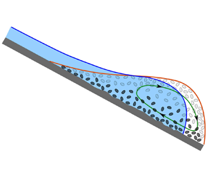
 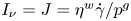 $I_\nu =J=\eta ^w\dot \gamma /p^g$, where
  $\dot \gamma$ is the shear rate and
  $p^g$ is the pressure due to grain contacts. This suspension rheology works well at low shear rates, but at higher shear rates, it has been found that there is a transition towards a dependence on the granular inertial number
  $I=\dot \gamma d/\sqrt {p^g/\varrho ^{g\star }}$ (Trulsson, Andreotti & Claudin Reference Trulsson, Andreotti and Claudin2012; Maurin, Chauchat & Frey Reference Maurin, Chauchat and Frey2016). While these suspension rheologies determine the composite response for a single effective medium, it is by no means clear how to partition the stress back between the individual phases.
Equations (2.6) and (2.7) are consistent with the mixture theory approach of Nunziato et al. (Reference Nunziato, Passman, Givler, Mactigue and Brady1986), although an ensemble averaging approach is also possible (Anderson & Jackson Reference Anderson and Jackson1967; Joseph & Lungdren Reference Joseph and Lungdren1990; Anderson, Sundaresan & Jackson Reference Anderson, Sundaresan and Jackson1995; Enwald, Pelrano & Almstedt Reference Enwald, Pelrano and Almstedt1996; Jackson Reference Jackson2000). The sum of the partial solid and fluid stresses, (2.5) and (2.6), determines the total stress
 \begin{equation} \boldsymbol{\sigma}^{total}={-}p^{w\star}\textbf{1}-\boldsymbol{\sigma}^{e}+\boldsymbol{\tau}^w, \end{equation}
which is consistent with the effective stress principle of soil mechanics (Terzaghi Reference Terzaghi1943). It also agrees with the experimental observation that the manometric pressure in the soil is the pressure as if the medium were a bulk fluid, unaffected by the presence of the solid constituent in the medium.
The interaction drags acting on the water and grain phases are defined by
 \begin{equation} \boldsymbol{\beta}^w={-}\boldsymbol{\beta}^g=p^{w\star}\boldsymbol{\nabla} \phi^w+C^d(\boldsymbol{u}^g-\boldsymbol{u}^w), \end{equation}
where the term  $p^{w\star }\boldsymbol {\nabla }\phi ^w$ combines with the partial water pressure gradient
  $-\boldsymbol {\nabla }(\phi ^w p^{w\star })$ in the water momentum balance (2.3) to ensure that the fluid is driven by gradients in the intrinsic pore water pressure
  $-\phi ^w\boldsymbol {\nabla } p^{w\star }$, consistent with Darcy's law (Bear Reference Bear1972; Morland Reference Morland1992). The second term on the right-hand side of (2.9) is the drag due to the relative motion of the grains and water, with drag coefficient
 \begin{equation} C^d=\eta^w\frac{(\phi^w)^2}{k}, \quad\hbox{where the permeability}\ k=\frac{(\phi^w)^3d^2}{180(\phi^g)^2}, \end{equation}
is given by Carman's formula for the packing of spheres of diameter  $d$. This agrees well with the sediment dynamics experiments of Goharzadeh, Khalili & Jørgensen (Reference Goharzadeh, Khalili and Jørgensen2005) and Ouriemi, Aussillous & Guazzelli (Reference Ouriemi, Aussillous and Guazzelli2009).
When the constitutive laws (2.5) and (2.6) and the interaction drags (2.9) are substituted into (2.3), the momentum balance equations for the grains and the fluid take the form
 $$\begin{gather} \frac{\partial}{\partial t}(\varrho^g\boldsymbol{u}^g)+ \boldsymbol{\nabla}\boldsymbol{\cdot}(\varrho^g\boldsymbol{u}^g\otimes\boldsymbol{u}^g) ={-}\boldsymbol{\nabla}\boldsymbol{\cdot}\boldsymbol{\sigma}^e - \phi^g\boldsymbol{\nabla} p^{w\star}+ \varrho^g\boldsymbol{g} + C^d(\boldsymbol{u}^w-\boldsymbol{u}^g), \end{gather}$$
 $$\begin{gather}\frac{\partial}{\partial t}(\varrho^w\boldsymbol{u}^w)+\boldsymbol{\nabla}\boldsymbol{\cdot} (\varrho^w\boldsymbol{u}^w\otimes\boldsymbol{u}^w)={-}\phi^w\boldsymbol{\nabla} p^{w\star}+\boldsymbol{\nabla}\boldsymbol{\cdot}\boldsymbol{\tau}^w+\varrho^w \boldsymbol{g}+C^d(\boldsymbol{u}^g-\boldsymbol{u}^w), \end{gather}$$
assuming that the mixture is fully saturated. When there is no water ( $\phi ^w=0$), the buoyancy force
  $-\phi ^g\boldsymbol {\nabla } p^{w\star }$ and the Darcy interaction force
 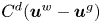 $C^d(\boldsymbol {u}^w-\boldsymbol {u}^g)$ are assumed to be zero, and the momentum balance (2.11) then reduces to that for dry grains. Conversely, in the case of pure water (
 $\phi ^w=1$), (2.12) naturally reduces to the Navier–Stokes equations. The momentum balances (2.11) and (2.12) are identical to those employed to investigate debris flows by Iverson & Denlinger (Reference Iverson and Denlinger2001), sediment flows by Ouriemi et al. (Reference Ouriemi, Aussillous and Guazzelli2009) and general fluid–sediment flows by Baumgarten & Kamrin (Reference Baumgarten and Kamrin2019), apart from the particular choices of the Darcy drag coefficients and effective fluid phase viscosity.
2.2. Boundary conditions
A Cartesian coordinate system  $Oxz$ is introduced with the
  $x$-axis pointing down a slope inclined at an angle
  $\zeta$ to the horizontal and with the
  $z$-axis pointing upwards, as shown in figure 2. A third coordinate
  $y$, lying across the slope, can easily be added to model fully three-dimensional flows, but for ease of exposition, the theory presented here is purely two-dimensional. The debris flow is assumed to have velocity components
  $\boldsymbol {u}^\nu =(u^\nu, w^\nu )$ in the downslope and slope normal directions, respectively. The grain surface is defined by the function
  $F^g(z,x,t)=z-s^g(x,t)$, the water surface by
  $F^w(z,x,t)=z-s^w(x,t)$ and the basal surface by
  $F^b(z,x,t)=z-b(x)$. It follows that the upward pointing unit normal for each surface is
  $\boldsymbol {n}^\nu =\boldsymbol {\nabla } F^\nu /\vert \boldsymbol {\nabla } F^\nu \vert$, where
  $\nu =g, w, b$. In the undersaturated regime (figure 2b), the water surface is below the grain surface, i.e.
  $s^w< s^g$, whereas in the oversaturated regime (figure 2c), the water surface is above it, i.e.
  $s^g< s^w$.

Figure 2. (a) Two-dimensional schematic diagram of a debris flow on a slope inclined at an angle  $\zeta$ to the horizontal. Blue shading corresponds to water, while the grains occupy the region below the red free surface. Velocity shear results in the surface layer of (light) grains moving towards the front, while the (dark) grains near the base move backwards relative to the front. This creates a recirculating (green) frontal cell. The water free surface (blue) and the granular free surface (red) do not coincide. The debris flow therefore consists of a dry granular front, an undersaturated wet flow, an oversaturated wet flow and a pure watery tail. It is useful to resolve the vertical structure as shown in panels (b,c) for the undersaturated and oversaturated regimes. In panel (b), the granular free surface at
  $z=s^g(x,t)$ is above the water free surface at
  $z=s^w(x,t)$, while in the oversaturated regime, the situation is reversed. The base of the flow lies at
  $z=b(x)$ and the water and grain heights are
  $h^w=s^w-b$ and
  $h^g=s^g-b$. The internal interface height is
  $\textrm {min}(h^g, h^w)$ and the proportion of the water flow height that is occupied by grains is equal to
  $\mathcal {H}=\textrm {min}(h^g, h^w)/h^w$. Within this vertical structure, region (i) consists of dry grains, region (ii) is a mixture of grains and water, and region (iii) is pure water.
The grain phase is subject to kinematic conditions on the grain surface  $F^g(x, t)=0$ and the basal surface
  $F^b(x)=0$. These conditions are given by
 $$\begin{gather} \frac{\partial F^g}{\partial t} + \boldsymbol{u}^g\boldsymbol{\cdot}\boldsymbol{\nabla} F^g = 0,\quad F^g(x, t)=0, \end{gather}$$
 $$\begin{gather}\frac{\partial F^b}{\partial t} + \boldsymbol{u}^g\boldsymbol{\cdot}\boldsymbol{\nabla} F^b = 0,\quad F^b(x)=0. \end{gather}$$
Similarly, the water phase is subject to kinematic conditions on the water surface  $F^w(x, t)=0$ and the basal surface
  $F^b(x)=0$. They are given by
 $$\begin{gather} \frac{\partial F^w}{\partial t} + \boldsymbol{u}^w\boldsymbol{\cdot}\boldsymbol{\nabla} F^w = 0,\quad F^w(x, t)=0, \end{gather}$$
 $$\begin{gather}\frac{\partial F^b}{\partial t} + \boldsymbol{u}^w\boldsymbol{\cdot}\boldsymbol{\nabla} F^b = 0,\quad F^b(x)=0. \end{gather}$$
Grains can penetrate the water surface in the undersaturated regime (figure 2b) and water can penetrate the grain surface in the oversaturated regime (figure 2c). The material that crosses these surfaces can change its volume fraction abruptly, e.g. in the oversaturated regime, the volume fraction of water jumps from  $\phi ^w=1-\phi ^g$ to
  $\phi ^w=1$ across the interface. To describe such singular interfaces, the mass jump conditions (Chadwick Reference Chadwick1976) are
 $$\begin{gather} \unicode{x27E6}\varrho^g(\boldsymbol{u}^g-\boldsymbol{u}^w)\boldsymbol{\cdot}\boldsymbol{n}^w \unicode{x27E7} = 0,\quad F^w(x, t)=0, \end{gather}$$
 $$\begin{gather}\unicode{x27E6}\varrho^w(\boldsymbol{u}^w-\boldsymbol{u}^g)\boldsymbol{\cdot}\boldsymbol{n}^g \unicode{x27E7} = 0,\quad F^g(x, t)=0, \end{gather}$$
where the jump brackets  $\unicode{x27E6} ~\unicode{x27E7}$ indicate the difference between the enclosed quantity on the forward (
 $+$) and rearward (
 $-$) sides of the discontinuity. Equation (2.17) describes the conservation of grains across the water free surface in the undersaturated case, while (2.18) describes the conservation of water across the granular free surface in the oversaturated regime.
Grains and water satisfy traction-free conditions at their free surfaces
 $$\begin{gather} \boldsymbol{\sigma}^e\boldsymbol{n}^g=\boldsymbol{0},\quad F^g(x, t)=0, \end{gather}$$
 $$\begin{gather}\boldsymbol{\sigma}^w\boldsymbol{n}^w=\boldsymbol{0},\quad F^w(x, t)=0. \end{gather}$$
Iverson (Reference Iverson2003) used large-scale debris flow flume tests to show that the grain phase experiences a Coulomb-type friction. Additionally, the Chézy formula (Chaudhry Reference Chaudhry2008), an empirically derived expression to take into account turbulent friction arising from the bottom of the channel, can be employed to describe the basal friction experienced by the water phase. The solid bed friction and Chézy formula take the form
 $$\begin{gather} \boldsymbol{\sigma}^e\boldsymbol{n}^b-(\boldsymbol{n}^b\boldsymbol{\cdot} \boldsymbol{\sigma}^e\boldsymbol{n}^b)\boldsymbol{n}^b ={-}\frac{\boldsymbol{u}^g_b}{|{\boldsymbol{u}^g_b}|}\mu^b(\boldsymbol{n}^b \boldsymbol{\cdot}\boldsymbol{\sigma}^e\boldsymbol{n}^b),\quad F^b(x)=0, \end{gather}$$
 $$\begin{gather}\boldsymbol{\sigma}^w\boldsymbol{n}^b-(\boldsymbol{n}^b\boldsymbol{\cdot} \boldsymbol{\sigma}^w\boldsymbol{n}^b)\boldsymbol{n}^b =\varrho^{w\star}C^w|{\bar{\boldsymbol{u}}}^{w}|\bar{\boldsymbol{u}}^{w},\quad F^b(x)=0, \end{gather}$$
where  $\mu ^b$ is the basal friction coefficient,
  $C^w$ is the Chézy drag coefficient (Hogg & Pritchard Reference Hogg and Pritchard2004) and
  $\bar {\boldsymbol {u}}^w$ is the depth-averaged water velocity. Detailed formulae for the coefficients
  $\mu ^b$ and
  $C^w$ will be discussed after the depth-integration process.
3. Non-dimensionalisation
3.1. Scaling the governing equations
Debris flows typically have a flow depth  $H$ that is much smaller than their length
  $L$. This makes it possible to derive a depth-averaged model, which does not depend on the normal coordinate
  $z$. Typical downstream flow speeds for both the grain and water phases are assumed to be of the order of the gravity wave speed
  $U=(gH)^{1/2}$, and the mass balances then imply that typical normal velocities are of magnitude
  $\varepsilon U$, where the aspect ratio
  $\varepsilon =H/L\ll 1$. Hydrostatic and lithostatic balances for the pore fluid pressure and the grain normal stresses suggest scalings of
  $\varrho ^{w\star }gH$ and
  $\varrho ^{g\star }gH$, respectively. A Coulomb friction law then suggests that the typical order of magnitude for the grain shear stress is
  $\mu \varrho ^{g\star }gH$, where
  $\mu$ is the friction coefficient. The scaling of the deviatoric water stress is determined by the Newtonian constitutive law (2.7). The governing equations and boundary conditions are therefore non-dimensionalised by the scalings
 \begin{equation} \left.\begin{gathered} (x,z,s^w, s^g, b, d)=L(\hat{x}, varepsilon\hat{z}, \varepsilon\hat{s}^w, \varepsilon\hat{s}^g, \varepsilon\hat{b}, \varepsilon\hat{d}),\quad t=L/(gH)^{1/2}\hat{t}, \\ (u^\nu, w^\nu, \vert\boldsymbol{u}^\nu\vert)=(gH)^{1/2}(\hat{u}^{\nu}, \varepsilon\hat{w}^{\nu}, \vert\hat{\boldsymbol{u}}^\nu\vert),\quad C^d=\varrho^{w\star}(g/H)^{1/2}\hat C^d,\\ (\sigma^e_{xx}, \sigma^e_{zz},\sigma^e_{xz})=\varrho^{g\star}gH(\hat{\sigma}^e_{xx}, \hat{\sigma}^e_{zz}, \mu\hat{\sigma}^e_{xz}) ,\\(p^{w\star}, \tau_{xx}^w, \tau_{zz}^w, \tau_{xz}^w) =\varrho^{w\star}gH(\hat{p}^{w\star}, \varepsilon\hat{\tau}_{xx}^w, \varepsilon\tau_{zz}^w, \hat{\tau}_{xz}^w), \end{gathered}\right\} \end{equation}
where the hatted quantities are non-dimensional. These scalings imply that for the grains, the non-dimensional mass and momentum balance components are
 \begin{align} &\hspace{5pc}\frac{\partial\phi^g}{\partial\hat{t}}+\frac{\partial}{\partial \hat{x}}(\phi^g\hat{u}^g)+ \frac{\partial}{\partial \hat{z}}(\phi^g\hat{w}^g)=0, \end{align}
 \begin{align} & \varepsilon\left(\frac{\partial}{\partial\hat{t}}(\phi^g\hat{u}^g)+ \frac{\partial}{\partial \hat{x}}(\phi^g\hat{u}^g\hat{u}^g)+ \frac{\partial}{\partial \hat{z}}(\phi^g\hat{u}^g\hat{w}^g)\right) \nonumber\\ &\quad ={-}\varepsilon\gamma\phi^g\frac{\partial \hat{p}^{w\star}}{\partial \hat{x}}-\varepsilon \frac{\partial\hat{\sigma}^e_{xx}}{\partial\hat{x}} -\mu\frac{\partial\hat{\sigma}^e_{xz}}{\partial\hat{z}}+\phi^g\sin\zeta+ \gamma\hat{C}^d(\hat{u}^w-\hat{u}^g), \end{align}
 \begin{align} & \varepsilon^2\left(\frac{\partial}{\partial\hat{t}}(\phi^g\hat{w}^g)+ \frac{\partial}{\partial \hat{x}}(\phi^g\hat{u}^g\hat{w}^g)+ \frac{\partial}{\partial \hat{z}}(\phi^g\hat{w}^g\hat{w}^g)\right) \nonumber\\ &\quad ={-}\gamma\phi^g\frac{\partial \hat{p}^{w\star}}{\partial \hat{z}}-\varepsilon\mu \frac{\partial\hat{\sigma}^e_{xz}}{\partial\hat{x}} -\frac{\partial\hat{\sigma}^e_{zz}}{\partial\hat{z}} -\phi^g\cos\zeta+\varepsilon\gamma\hat{C}^d(\hat{w}^w-\hat{w}^g), \end{align}
where the density ratio
 \begin{equation} \gamma = \varrho^{w\star}/\varrho^{g\star}. \end{equation}
Similarly, the non-dimensional water mass balance and the downslope and normal components of the momentum balance are given by
 \begin{align} & \hspace{5pc}\frac{\partial\phi^w}{\partial\hat{t}}+\frac{\partial}{\partial \hat{x}}(\phi^w\hat{u}^w)+ \frac{\partial}{\partial \hat{z}}(\phi^w\hat{w}^w)=0, \end{align}
 \begin{align} & \varepsilon\left(\frac{\partial}{\partial\hat{t}}(\phi^w\hat{u}^w)+ \frac{\partial}{\partial \hat{x}}(\phi^w\hat{u}^w\hat{u}^w)+ \frac{\partial}{\partial \hat{z}}(\phi^w\hat{u}^w\hat{w}^w)\right) \nonumber\\ &\quad ={-}\varepsilon\phi^w\frac{\partial \hat{p}^{w\star}}{\partial \hat{x}}+\varepsilon^2 \frac{\partial\hat{\tau}^w_{xx}}{\partial\hat{x}}+\frac{\partial\hat{\tau}^w_{xz}}{\partial\hat{z}} +\phi^w\sin\zeta-\hat{C}^d(\hat{u}^w-\hat{u}^g), \end{align}
 \begin{align} & \varepsilon^2\left(\frac{\partial}{\partial\hat{t}}(\phi^w\hat{w}^w)+ \frac{\partial}{\partial \hat{x}}(\phi^w\hat{u}^w\hat{w}^w)+ \frac{\partial}{\partial \hat{z}}(\phi^w\hat{w}^w\hat{w}^w)\right) \nonumber\\ &\quad ={-}\phi^w\frac{\partial \hat{p}^{w\star}}{\partial \hat{z}}+\varepsilon \frac{\partial\hat{\tau}^w_{xz}}{\partial\hat{x}}+\varepsilon\frac{\partial\hat{\tau}^w_{zz}}{\partial\hat{z}} -\phi^w\cos\zeta-\varepsilon\hat{C}^d(\hat{w}^w-\hat{w}^g). \end{align}
3.2. Non-dimensional boundary conditions
The non-dimensional kinematic conditions (2.13) and (2.14) for the grains are
 $$\begin{gather} \frac{\partial \hat{s}^g}{\partial\hat{t}} + \hat{u}^g\frac{\partial\hat{s}^g}{\partial\hat{x}}-\hat{w}^g=0,\quad \hat{z}=\hat{s}^g(\hat{x},\hat{t}), \end{gather}$$
 $$\begin{gather}\frac{\partial \hat{b}}{\partial\hat{t}} + \hat{u}^g\frac{\partial\hat{b}}{\partial\hat{x}}-\hat{w}^g=0,\quad \hat{z}=\hat{b}(\hat{x}), \end{gather}$$
and the non-dimensional kinematic conditions (2.15) and (2.16) for the water are
 $$\begin{gather} \frac{\partial \hat{s}^w}{\partial\hat{t}} + \hat{u}^w\frac{\partial\hat{s}^w}{\partial\hat{x}}-\hat{w}^w=0,\quad \hat{z}=\hat{s}^w(\hat{x},\hat{t}), \end{gather}$$
 $$\begin{gather}\frac{\partial \hat{b}}{\partial\hat{t}} + \hat{u}^w\frac{\partial\hat{b}}{\partial\hat{x}}-\hat{w}^w=0,\quad \hat{z}=\hat{b}(\hat{x}). \end{gather}$$
 To formulate the non-dimensional form of the mass-jump conditions (2.17) and (2.18), the kinematic conditions (2.15) and (2.13) are used to show that  $\boldsymbol {u}^w\boldsymbol {\cdot }\boldsymbol {n}^w=-(\partial F^w/\partial t){\cdot} (1/\vert \boldsymbol {\nabla } F^w\vert )$ and
  $\boldsymbol {u}^g\boldsymbol {\cdot }\boldsymbol {n}^g=-(\partial F^g/\partial t)\cdot (1/\vert \boldsymbol {\nabla } F^g\vert )$. Substitution of these results implies that the non-dimensional jump conditions at the undersaturated water free surface and the oversaturated grain free surface are
 $$\begin{gather} \left[\!\!\left[ \phi^{g}\left(\frac{\partial\hat{s}^w}{\partial\hat{t}}+\hat{u}^{g} \frac{\partial\hat{s}^w}{\partial\hat{x}}-\hat{w}^{g}\right)\right]\!\!\right]=0,\quad \hat{z}=\hat{s}^w(\hat x,\hat t), \end{gather}$$
 $$\begin{gather}\left[\!\!\left[\phi^{w}\left(\frac{\partial\hat{s}^g}{\partial\hat{t}}+\hat{u}^{w} \frac{\partial\hat{s}^g}{\partial\hat{x}}-\hat{w}^{w}\right)\right]\!\!\right]=0,\quad \hat{z}=\hat{s}^g(\hat x,\hat t). \end{gather}$$
The non-dimensional downslope and normal components of the grain surface traction (2.19) are
 $$\begin{gather} -\varepsilon\hat{\sigma}^e_{xx}\frac{\partial\hat{s}^g}{\partial\hat{x}}+\mu\hat{\sigma}_{xz}^e=0,\quad \hat{z}=\hat{s}^g(\hat{x},\hat{t}), \end{gather}$$
 $$\begin{gather}-\varepsilon\mu\hat{\sigma}^e_{xz}\frac{\partial\hat{s}^g}{\partial\hat{x}}+\hat{\sigma}^e_{zz}=0,\quad \hat{z}=\hat{s}^g(\hat{x},\hat{t}), \end{gather}$$
and the non-dimensional components of the water surface traction (2.20) are
 $$\begin{gather} \varepsilon\phi^w\hat{p}^{w\star}\frac{\partial\hat{s}^w}{\partial\hat{x}}-\varepsilon^2\hat{\tau}^w_{xx} \frac{\partial\hat{s}^w}{\partial\hat{x}}+\hat{\tau}^w_{xz}=0,\quad \hat{z}=\hat{s}^w(\hat{x},\hat{t}), \end{gather}$$
 $$\begin{gather}-\phi^w\hat{p}^{w\star}-\varepsilon\hat{\tau}^w_{xz}\frac{\partial\hat{s}^w}{\partial\hat{x}}+ \varepsilon\hat{\tau}^w_{zz}=0,\quad \hat{z}=\hat{s}^w(\hat{x},\hat{t}). \end{gather}$$
The downslope and normal components of the basal granular traction (2.21) are
 $$\begin{gather} -\varepsilon\hat{\sigma}_{xx}^e\frac{\partial\hat{b}}{\partial\hat{x}} + \mu\hat{\sigma}^e_{xz} ={-}(\boldsymbol{n}^b\boldsymbol{\cdot}\hat{\boldsymbol{\sigma}}^e\boldsymbol{n}^b) \left(\frac{\hat{u}_b^g}{\vert\hat{\boldsymbol{u}}_b^g\vert}\mu^b|\boldsymbol{\nabla} F^b|+\varepsilon \frac{\partial\hat{b}}{\partial\hat{x}}\right),\quad \hat{z}=\hat{b}(\hat{x}), \end{gather}$$
 $$\begin{gather}-\varepsilon\mu\hat{\sigma}^e_{zx}\frac{\partial\hat{b}}{\partial\hat{x}} + \hat{\sigma}^e_{zz} ={-}(\boldsymbol{n}^b\boldsymbol{\cdot}\hat{\boldsymbol{\sigma}}^e\boldsymbol{n}^b) \left(\varepsilon\frac{\hat{w}^g_b}{|{\hat{\boldsymbol{u}}^g_b}|}\mu^b|\boldsymbol{\nabla} F^b|-1\right),\quad \hat{z}=\hat{b}(\hat{x}), \end{gather}$$
where  $|\hat {\boldsymbol {u}}_b^g|=\sqrt {(\hat {u}_b^g)^2 + \varepsilon ^2(\hat {w}_b^g)^2}$ and
  $|\boldsymbol {\nabla } F^b|=\sqrt {1+\varepsilon ^2(\partial \hat b/\partial \hat x)^2}$. Similarly, the downslope and normal components of the water basal friction (2.22) are
 $$\begin{gather} -\varepsilon^2\hat{\tau}_{xx}^w\frac{\partial\hat{b}}{\partial\hat{x}}+\hat{\tau}_{xz}^w+\varepsilon \left(\phi^w\hat{p}^{w\star}_b+(\boldsymbol{n}^b\boldsymbol{\cdot} \hat{\boldsymbol{\sigma}}^w\boldsymbol{n}^b)\right) \frac{\partial\hat{b}}{\partial\hat{x}}=C^w\hat{\bar{u}}^w|{\hat{\bar{\boldsymbol{u}}}^w}\|\boldsymbol{\nabla} F^b|,\quad \hat{z}=\hat{b}(\hat{x}), \end{gather}$$
 $$\begin{gather}-\varepsilon\hat{\tau}_{zx}^w\frac{\partial\hat{b}}{\partial\hat{x}}+\varepsilon \hat{\tau}_{zz}^w-\left(\phi^w\hat{p}^{w\star}_b+(\boldsymbol{n}^b\boldsymbol{\cdot} \hat{\boldsymbol{\sigma}}^w\boldsymbol{n}^b)\right)=\varepsilon C^w\hat{\bar{w}}^w|{\hat{\bar{\boldsymbol{u}}}^w}\|\boldsymbol{\nabla} F^b|,\quad \hat{z}=\hat{b}(\hat{x}), \end{gather}$$
where  $|\hat {\bar {\boldsymbol {u}}}^w|=\sqrt {(\hat {\bar {u}}^w)^2 + \varepsilon ^2(\hat {\bar {w}}^w)^2}$.
4. Depth integration
4.1. Depth-averaged mass balance equations
The mass balance equations (3.2) and (3.6) can be integrated through the flow depth using Leibniz’s rule (Abramowitz & Stegun Reference Abramowitz and Stegun1970) to exchange the order of differentiation and integration, and then simplified by using the kinematic conditions (3.9)–(3.12). In the oversaturated regime, the standard argument (Savage & Hutter Reference Savage and Hutter1989; Gray et al. Reference Gray, Wieland and Hutter1999) is complicated by the jump in the water volume fraction at the internal free surface of the grains. To overcome this, the integration of (3.6) is divided into two parts, which implies that the depth-integrated water mass balance is
 \begin{equation} \frac{\partial}{\partial\hat{t}}(\hat{h}^w\bar{\phi}^w)+ \frac{\partial}{\partial\hat{x}}(\hat{h}^w\overline{\phi^w{\hat{u}}^w}) +\left[\!\!\left[\phi^{w}\left(\frac{\partial\hat{s}^g}{\partial\hat{t}}+\hat{u}^{w} \frac{\partial\hat{s}^g}{\partial\hat{x}}-\hat{w}^{w}\right)\right]\!\!\right]=0, \end{equation}
where the jump bracket is evaluated at  $\hat z=\hat s^g$, the water thickness
  $\hat {h}^w=\hat {s}^w-\hat {b}$, and the depth-averaged water concentration and depth-averaged water flux are
 \begin{equation} \bar{\phi}^w=\frac{1}{\hat{h}^w}\int_{\hat{b}}^{\hat{s}^w}\phi^wd\hat{z},\quad \overline{\phi^w\hat{u}^w}=\frac{1}{\hat{h}^w}\int_{\hat{b}}^{\hat{s}^w}\phi^w{\hat{u}}^wd\hat{z}, \end{equation}
respectively. The jump bracketed term in (4.1) is zero by the water mass jump condition (3.14), so the depth-averaged water mass balance reduces to standard form, despite the jump in concentration. A similar argument carries through in the same way for the depth-averaged grain mass balance in the undersaturated regime. As a result, the depth-averaged grain and water mass balances are
 $$\begin{gather} \frac{\partial}{\partial\hat{t}}(\hat{h}^g\bar{\phi}^g)+ \frac{\partial}{\partial\hat{x}}(\hat{h}^g\overline{\phi^g{\hat{u}}^g})=0, \end{gather}$$
 $$\begin{gather}\frac{\partial}{\partial\hat{t}}(\hat{h}^w\bar{\phi}^w)+ \frac{\partial}{\partial\hat{x}}(\hat{h}^w\overline{\phi^w{\hat{u}}^w})=0, \end{gather}$$
where the granular flow thickness  $\hat h^g=\hat s^g-\hat b$ and
 \begin{equation} \bar{\phi}^g=\frac{1}{\hat{h}^g}\int_{\hat{b}}^{\hat{s}^g}\phi^gd\hat{z},\quad \overline{\phi^g\hat{u}^g}=\frac{1}{\hat{h}^g}\int_{\hat{b}}^{\hat{s}^g}\phi^g{\hat{u}}^gd\hat{z}. \end{equation}
To further simplify (4.3) and (4.4), the vertical distributions of the solid and water volume fractions must be prescribed. The simplest approach is to assume that  $\phi ^g$ is constant, regardless of whether the flow is undersaturated or oversaturated, i.e.
 \begin{equation} \phi^g=\phi^c. \end{equation}
This is assumed in early debris flow models (Iverson Reference Iverson1997; Iverson & Denlinger Reference Iverson and Denlinger2001) and appears to be a good approximation in high solids volume fraction granular-dominated flows (Maurin et al. Reference Maurin, Chauchat and Frey2016; Chassagne et al. Reference Chassagne, Maurin, Chauchat, Gray and Frey2020). However, when the fluid can suspend grains, the solids volume fraction increases with depth (Egashira, Itoh & Takeuchi Reference Egashira, Itoh and Takeuchi2001; Maurin et al. Reference Maurin, Chauchat and Frey2016) and this will not be a good approximation. The fact that  $\phi ^c$ is constant and uniform throughout the debris flow precludes pore pressure effects (Iverson & George Reference Iverson and George2014). There is therefore potential to improve the model (at this point) in future. The exclusion of pore pressure effects does, however, allow us to show that they are not necessarily needed to drive the forward motion of grains from an oversaturated tail towards the flow front, which is the traditional view in the debris flow community.
As sketched in figure 2(b,c) the volume fraction of water is assumed to have a vertical distribution that is dependent on whether the flow is undersaturated or oversaturated. In the undersaturated regime,
 \begin{equation} \phi^w=\left\{\begin{array}{ll} 0, & \hat z\in[\hat s^w,\hat s^g],\\ 1-\phi^c, & \hat z\in[\hat b,\hat s^w], \end{array}\right. \end{equation}
while in the oversaturated regime,
 \begin{equation} \phi^w=\left\{\begin{array}{ll} 1, & \hat z\in[\hat s^g,\hat s^w],\\ 1-\phi^c, & \hat z\in[\hat b,\hat s^g]. \end{array}\right. \end{equation}
It is useful to define volume-fraction-weighted depth-averaged velocities
 \begin{equation} \hat{\bar{u}}^g=\frac{\displaystyle\int_{\hat{b}}^{\hat{s}^g}\phi^g\hat{u}^g\,\text{d}\hat{z}}{\displaystyle \int_{\hat{b}}^{\hat{s}^g}\phi^g\,\text{d}\hat{z}}=\frac{\overline{\phi^g{\hat{u}}^g}}{\bar{\phi}^g},\quad \hat{\bar{u}}^w=\frac{\displaystyle\int_{\hat{b}}^{\hat{s}^w}\phi^w\hat{u}^w\,\text{d}\hat{z}}{\displaystyle \int_{\hat{b}}^{\hat{s}^w}\phi^w\,\text{d}\hat{z}}=\frac{\overline{\phi^w{\hat{u}}^w}}{\bar{\phi}^w}. \end{equation}
Since the solids volume fraction is constant, (4.9a) reduces to the standard definition (Savage & Hutter Reference Savage and Hutter1989; Gray et al. Reference Gray, Wieland and Hutter1999; Pitman & Le Reference Pitman and Le2005; Gray & Edwards Reference Gray and Edwards2014). This is also true for the water in the undersaturated regime, but in the oversaturated regime, the internal concentration discontinuity (4.8) implies that the definition of the depth-averaged water velocity (4.9b) is different. Using the definitions (4.6)–(4.9a,b), it follows that the depth-averaged mass balance of the grains in both the undersaturated and oversaturated regimes is
 \begin{equation} \frac{\partial}{\partial\hat{t}}(\hat{h}^g\phi^c) + \frac{\partial}{\partial\hat{x}} (\hat{h}^g\phi^c\hat{\bar{u}}^g)=0, \end{equation}
while the depth-averaged mass balances for the water in the undersaturated and oversaturated regimes are
 $$\begin{gather} \frac{\partial}{\partial\hat{t}}(\hat{h}^w(1-\phi^c))+ \frac{\partial}{\partial\hat{x}}(\hat{h}^w(1-\phi^c)\hat{\bar{u}}^w)=0, \end{gather}$$
 $$\begin{gather}\frac{\partial}{\partial\hat{t}}(\hat{h}^w(1-\phi^c\hat{h}^g/\hat{h}^w))+ \frac{\partial}{\partial\hat{x}}(\hat{h}^w(1-\phi^c\hat{h}^g/\hat{h}^w)\hat{\bar{u}}^w)=0, \end{gather}$$
respectively. The factors  $\phi ^c$ and
  $1-\phi ^c$ in (4.10) and (4.11) are constants that could be cancelled out. However, these factors are retained here to develop a theoretical framework that can switch seamlessly between regimes.
4.2. Normal components of the momentum equations
The normal components of the momentum balances play a crucial role in deriving normal stresses in depth-averaged models (Savage & Hutter Reference Savage and Hutter1989; Iverson & Denlinger Reference Iverson and Denlinger2001; Gray & Edwards Reference Gray and Edwards2014). To leading order in  $\varepsilon$, the water normal momentum balance (3.8) implies that the fluid pressure is hydrostatic
 \begin{equation} \frac{\partial\hat{p}^{w\star}}{\partial \hat{z}}={-}\cos\zeta, \end{equation}
in both the mixed (ii) and pure water (iii) regions shown in figure 2(b,c). Excess pore pressure, which is important in large-scale debris flows containing fine particles (Iverson et al. Reference Iverson, Logan, Lahusen and Berti2010), is therefore neglected in this model. In the dry region (i), the water pressure and the Darcy drag vanish, and to leading order, the dry grain normal momentum balance (3.4) reduces to
 \begin{equation} \frac{\partial\hat{\sigma}_{zz}^e}{\partial \hat{z}} ={-}\phi^c\cos\zeta, \end{equation}
while in the mixed region (ii), the saturated grain normal stress gradient balances gravity and buoyancy
 \begin{equation} \frac{\partial\hat{\sigma}_{zz}^e}{\partial \hat{z}} ={-}\phi^c\cos\zeta-\gamma\phi^c\displaystyle\frac{\partial\hat{p}^{w\star}}{\partial\hat{z}}. \end{equation}
Equations (4.13)–(4.15), together with their respective boundary conditions, enable expressions for the pore fluid pressure and the grain normal stress to be derived, as presented below.
4.3. Undersaturated pore fluid pressure and grain normal stress
To leading order, the surface condition (3.18) reduces to
 \begin{equation} \hat{p}^{w\star}(\hat{s}^w)=0. \end{equation}
The integration of (4.13) subject to (4.16) implies that the water pressure is hydrostatic
 \begin{equation} \hat{p}^{w\star}=(\hat{s}^w-\hat{z})\cos\zeta,\quad \hat{z}\in [\hat b,\hat{s}^w]. \end{equation}
It follows that the pore fluid pressure on the base is
 \begin{equation} \hat{p}^{w\star}_b=\hat{h}^w\cos\zeta, \end{equation}
and that the depth-averaged water pressure is
 \begin{equation} \hat{\bar{p}}^{w\star}=\frac{1}{\hat{h}^w}\int_{\hat{b}}^{\hat{s}^w}\hat{p}^{w\star}\,\text{d}\hat{z}= \frac{1}{2}\hat{h}^w\cos\zeta. \end{equation}
 To leading order, the grain surface condition (3.16) implies that the surface stress  $\hat {\sigma }_{zz}^e$ vanishes. It follows that integrating (4.14) implies that the perpendicular grain normal stress in the dry region (i) is
 \begin{equation} \hat{\sigma}_{zz}^e=(\hat{s}^g-\hat{z})\phi^c\cos\zeta,\quad \hat z\in[\hat{s}^w,\hat{s}^g], \end{equation}
and hence that the perpendicular grain normal stress in the upper side of the water surface is  $\hat {\sigma }_{zz}^{e+}=(\hat {s}^g-\hat {s}^w)\phi ^c\cos \zeta$. Appendix A shows that provided the granular velocity profile through the depth of the flow is continuous, then there is no jump in the normal effective stress, and hence
 \begin{equation} \hat{\sigma}_{zz}^{e-}=\hat{\sigma}_{zz}^{e+}=(\hat{s}^g-\hat{s}^w)\phi^c\cos\zeta,\quad \hat z=\hat s^w. \end{equation}
In the saturated regime (ii), substitution of (4.13) into (4.15) implies that
 \begin{equation} \frac{\partial\hat{\sigma}_{zz}^e}{\partial \hat{z}}={-}\phi^c(1-\gamma)\cos\zeta,\quad \hat{z}\in [\hat b,\hat{s}^w]. \end{equation}
Integration of (4.22) subject to the continuity condition (4.21) implies that the perpendicular grain normal stress in the saturated regime (ii) is
 \begin{equation} \hat{\sigma}_{zz}^e=(\hat{s}^g-\hat{z})\phi^c\cos\zeta-(\hat{s}^w-\hat{z})\gamma\phi^c\cos\zeta,\quad \hat{z}\in[\hat b,\hat{s}^w], \end{equation}
and hence on the base,
 \begin{equation} \hat{\sigma}_{zz}^e(b) = (\hat{h}^g-\gamma\hat{h}^w)\phi^c\cos\zeta,\quad \hat z=\hat b. \end{equation}
The depth-averaged perpendicular grain normal stress is
 \begin{equation} \hat{\bar{\sigma}}_{zz}^e=\frac{1}{\hat{h}^g}\left(\int_{\hat{b}}^{\hat{s}^w}\hat{\sigma}^e_{zz}d\hat{z}+ \int_{\hat{s}^w}^{\hat{s}^g}\hat{\sigma}^e_{zz}\,\text{d}\hat{z}\right)= \frac{1}{2}\hat{h}^g\phi^c\cos\zeta-\frac{1}{2}\gamma(\hat{h}^w/\hat{h}^g)^2\hat{h}^g\phi^c\cos\zeta, \end{equation}
which, provided the earth pressure coefficient is equal to unity (Savage & Hutter Reference Savage and Hutter1989; Gray et al. Reference Gray, Wieland and Hutter1999; Pouliquen Reference Pouliquen1999a), implies that the depth-averaged downslope grain normal stress is
 \begin{equation} \hat{\bar{\sigma}}_{xx}^e=\tfrac{1}{2}\hat{h}^g\phi^c\cos\zeta-\tfrac{1}{2} \gamma(\hat{h}^w/\hat{h}^g)^2\hat{h}^g\phi^c\cos\zeta. \end{equation}
It follows that to leading order, (3.20) implies that the basal normal stress
 \begin{equation} \boldsymbol{n}^b\boldsymbol{\cdot}\hat{\boldsymbol{\sigma}}^e\boldsymbol{n}^b=\hat{\sigma}^e_{zz}(b) = \hat{h}^g(1-\gamma\hat{h}^w/\hat{h}^g)\phi^c\cos\zeta,\quad \hat z=\hat b. \end{equation}
4.4. Oversaturated pore fluid pressure and grain normal stress
Since (4.13) is independent of  $\phi ^w$, it can be integrated in the same way as the undersaturated case to show that the pressure is hydrostatic
 \begin{equation} \hat{p}^{w\star}=(\hat{s}^w-\hat{z})\cos\zeta. \end{equation}
Similarly, the basal water pressure and the depth-averaged water pressure are the same as the undersaturated case
 \begin{equation} \hat{p}^{w\star}_b=\hat{h}^w\cos\zeta,\quad \hat{\bar{p}}^{w\star}=\tfrac{1}{2}\hat{h}^w\cos\zeta, \end{equation}
and the pore fluid pressure at the grain surface is
 \begin{equation} \hat{p}^{w\star}(\hat{s}^g)=(\hat{h}^w-\hat{h}^g)\cos\zeta,\quad \hat{z}=\hat{s}^g. \end{equation}
To leading order, the traction-free condition (3.16) reduces to  $\hat {\sigma }_{zz}^e(\hat {s}^g)=0$. Substituting the gradient of the pore fluid pressure (4.13) into (4.15) and then integrating implies the perpendicular grain normal stress is
 \begin{equation} \hat{\sigma}_{zz}^e=(1-\gamma)(\hat{s}^g-\hat{z})\phi^c\cos\zeta,\quad \hat{z}\in[\hat b,\hat{s}^g], \end{equation}
and hence that the perpendicular basal normal stress is
 \begin{equation} \hat{\sigma}_{zz}^e(\hat{b}) = (1-\gamma)\hat{h}^g\phi^c\cos\zeta\quad \hat z=\hat b. \end{equation}
The depth-averaged perpendicular normal stress is then
 \begin{equation} \hat{\bar{\sigma}}_{zz}^e=\frac{1}{\hat{h}^g}\int_{\hat{b}}^{\hat{s}^g}\hat{\sigma}_{zz}^ed\hat{z}= \frac{1}{2}(1-\gamma)\hat{h}^g\phi^c\cos\zeta. \end{equation}
Given that the earth pressure coefficient is unity, the depth-averaged downslope normal stress is therefore equal to its counterpart in the vertical direction, i.e.
 \begin{equation} \hat{\bar{\sigma}}_{xx}^e=\tfrac{1}{2}(1-\gamma)\hat{h}^g\phi^c\cos\zeta. \end{equation}
To leading order, (3.20) shows the basal normal stress
 \begin{equation} \boldsymbol{n}^b\boldsymbol{\cdot}\hat{\boldsymbol{\sigma}}^e\boldsymbol{n}^b = \hat{\sigma}_{zz}^e(\hat{b})=(1-\gamma)\hat{h}^g\phi^c\cos\zeta. \end{equation}
4.5. Undersaturated depth-averaged downslope momentum balances
The downslope grain momentum balance (3.3) is now integrated from the bed  $\hat {z}=\hat {b}$ to the grain surface
  $\hat {z}=\hat {s}^g$. The integration is divided into two parts, because the buoyancy and Darcy drag are active only below the water surface
  $\hat {z}=\hat {s}^w$. Leibniz’s integration rule is used to swap the order of differentiation and integration, and the surface and basal kinematic conditions, (3.9) and (3.10), and downslope surface traction (3.15) are used to simplify the resulting equations. The calculations are lengthy and are therefore shown in Appendix B. The resulting depth-averaged momentum balance for the grains is
 \begin{align} & \varepsilon\left(\frac{\partial}{\partial\hat{t}}(\hat{h}^g\overline{\phi^g\hat{u}^g}) +\frac{\partial}{\partial\hat{x}}(\hat{h}^g\overline{\phi^g(\hat{u}^g)^2}) +\frac{\partial}{\partial\hat{x}}(\hat{h}^g\hat{\bar{\sigma}}_{xx}^e) +\gamma\phi^c\frac{\partial}{\partial\hat{x}}(\hat{h}^w\hat{\bar{p}}^w)\right) \nonumber\\ &\quad =\hat{h}^g\phi^c\sin\zeta - \left(\varepsilon\hat{\sigma}_{xx}^e(\hat b) \frac{\partial\hat{b}}{\partial\hat{x}}-\mu\hat{\sigma}_{xz}^{e}(\hat b)\right) -\gamma\hat{C}^d\int_{\hat{b}}^{\hat{s}^w}(\hat{u}^g-\hat{u}^w)\,\text{d}\hat{z} -\varepsilon\gamma\phi^c\hat{p}^{w\star}_b\frac{\partial\hat{b}}{\partial\hat{x}}. \end{align}
Substituting (4.27) into (3.19) implies that the basal downslope traction
 \begin{align} \varepsilon\hat{\sigma}_{xx}^e(\hat b)\frac{\partial\hat{b}}{\partial\hat{x}}-\mu\hat{\sigma}_{xz}^{e}(\hat b) &= \frac{\hat{u}^g_b}{|\hat{\boldsymbol{u}}^g_b|}(1-\gamma\hat{h}^w/\hat{h}^g)\mu^b\hat{h}^g\phi^c\cos\zeta \nonumber\\ &\quad +\varepsilon(1-\gamma{\hat{h}^w}/\hat{h}^g)\hat{h}^g\phi^c\cos\zeta \frac{\partial\hat{b}}{\partial\hat{x}}+O(\varepsilon^2), \end{align}
where the factor  $\hat {u}^g_b/|\hat {\boldsymbol {u}}^g_b|$ will be approximated as
  $\hat {\bar {u}}^g/|\hat {\bar {u}}^g|$. This approximation is employed in virtually all depth-averaged granular flow models (see e.g. Savage & Hutter Reference Savage and Hutter1989; Pitman & Le Reference Pitman and Le2005; Pudasaini Reference Pudasaini2012; Gray & Edwards Reference Gray and Edwards2014; Iverson & George Reference Iverson and George2014). To simplify the momentum transport terms, it is assumed that
 \begin{equation} \overline{\phi^g(\hat{u}^g)^2}=\frac{1}{\hat{h}^g}\int_{\hat{b}}^{\hat{s}^g} \phi^g(\hat{u}^g)^2\,\text{d}\hat{z}=\chi^g\bar\phi^g(\hat{\bar{u}}^g)^2, \end{equation}
where the shape factor  $\chi ^g$ for specific velocity profiles will be considered in § 4.8. It is also useful to define the streamfunction for the grains
 \begin{equation} \hat\psi^g(\hat z)=\int_{\hat{b}}^{\hat{z}} \hat{u}^g(\hat z')\,\text{d}\hat z', \end{equation}
which allows the Darcy drag exerted on the grain phase to be expressed as
 \begin{equation} \gamma\hat{C}^d\int_{\hat{b}}^{\hat{s}^w}(\hat{u}^g-\hat{u}^w)\,\text{d}\hat{z}= \gamma\hat{C}^d(\hat{\psi}^g(\hat s^w)-\hat{h}^w\hat{\bar{u}}^w). \end{equation}
 The gravitational force, the basal friction and the Darcy drag are all order unity quantities, but their sum is an order  $\varepsilon$ quantity. To express this theoretically, the leading order balance
  $\hat {\mathcal {L}}^g$ is defined as
 \begin{equation} \varepsilon\hat{\mathcal{L}}^g = \underbrace{\hat{h}^g\phi^c\sin\zeta}_{Gravity} -\underbrace{\mu^b\frac{\hat{\bar{u}}^g}{|\hat{\bar{u}}^g|} \left(1-\gamma\frac{\hat{h}^w}{\hat{h}^g}\right)\hat{h}^g\phi^c\cos\zeta}_{Basal\ friction} -\underbrace{\gamma\hat{C}^d(\hat{\psi}^g(\hat s^w)-\hat{h}^w\hat{\bar{u}}^w)}_{Darcy\ drag}. \end{equation}
When (4.6), (4.9a), (4.37), (4.38) and (4.41) are substituted into (4.36), together with the basal pressure (4.18), the depth-averaged pore fluid pressure (4.19) and the depth-averaged normal stress (4.26), the leading-order depth-averaged grain momentum balance in the undersaturated regime becomes
 \begin{equation} \frac{\partial}{\partial\hat{t}}(\hat{h}^g\phi^c\hat{\bar{u}}^g) + \frac{\partial }{\partial \hat{x}}\left(\chi^g \hat{h}^g\phi^c(\hat{\bar{u}}^g)^2+ {\frac{1}{2}(\hat{h}^g)^2\phi^c\cos\zeta}-{\frac{1}{2}\gamma (\hat{h}^w)^2\phi^c\cos\zeta}\right)=\hat{S}^g, \end{equation}
where the source terms
 \begin{equation} \hat{S}^g=\hat{\mathcal{L}}^g -\underbrace{\gamma\hat{h}^w\phi^c\cos\zeta\frac{\partial\hat{h}^w}{\partial\hat{x}}}_{{Buoyancy}} -\underbrace{\hat{h}^g\phi^c\cos\zeta\frac{\partial\hat{b}}{\partial\hat{x}}}_{{Topographic\ gradient}}, \end{equation}
combine the leading order balance (4.41) with the lower order buoyancy and topographic gradient terms. Note that the gradient of  $(1/2)\gamma (\hat {h}^w)^2\phi ^c\cos \zeta$ in (4.42) can be cancelled with the buoyancy term in (4.43). However, the equations are left in their present form to unify all the regimes in § 4.7.
Integrating the downslope water momentum balance (3.7) from the bed  $\hat {z}=\hat {b}$ to the water surface
  $\hat {z}=\hat {s}^w$ is more straightforward, because the integration does not pass through a singular surface. Using Leibniz’s integration rule to exchange the order of differentiation and integration and using the kinematic conditions (3.11) and (3.12), the surface traction (3.17) and the Darcy drag (4.40), the depth-averaged downslope water momentum balance is
 \begin{align} & \varepsilon\left(\frac{\partial}{\partial\hat{t}}(\hat{h}^w(1-\phi^c)\hat{\bar{u}}^w) +\frac{\partial}{\partial\hat{x}}(\chi^w\hat{h}^w(1-\phi^c)(\hat{\bar{u}}^w)^2) +(1-\phi^c)\frac{\partial}{\partial\hat{x}}(\hat{h}^w\hat{\bar{p}}^{w\star})\right) \nonumber\\ &\quad -\varepsilon^2\frac{\partial}{\partial\hat{x}}(\hat{h}^w\hat{\bar{\tau}}^w_{xx}) =\hat{h}^w(1-\phi^c)\sin\zeta-\hat{C}^d(\hat{h}^w\hat{\bar{u}}^w-\hat{\psi}^g(\hat s^w)) -\varepsilon(1-\phi^c)\hat{p}^{w\star}_b\frac{\partial\hat{b}}{\partial\hat{x}} \nonumber\\ &\quad +\left(\varepsilon^2\hat{\tau}_{xx}^w(\hat{b}) \frac{\partial\hat{b}}{\partial \hat{x}}-\hat{\tau}_{xz}^w(\hat{b})\right), \end{align}
where the water shape factor  $\chi ^w$ is defined as
 \begin{equation} \overline{\phi^w(\hat{u}^w)^2}=\frac{1}{\hat{h}^w} \int_{\hat{b}}^{\hat{s}^w}\phi^w(\hat{u}^w)^2\,\text{d}\hat{z}=\chi^w\bar\phi^w(\hat{\bar{u}}^w)^2. \end{equation}
The depth-averaged in-plane viscous stress  $\hat {\bar {\tau }}^w_{xx}$ is smaller than the other forces, and is usually neglected (Savage & Hutter Reference Savage and Hutter1989; Pitman & Le Reference Pitman and Le2005). However, it plays a crucial role in some subtle situations, including (i) obtaining the correct cutoff frequency of roll waves (Forterre Reference Forterre2006; Gray & Edwards Reference Gray and Edwards2014), (ii) generating cross-stream velocity profiles (Iverson & Denlinger Reference Iverson and Denlinger2001; Baker, Johnson & Gray Reference Baker, Johnson and Gray2016b; Meng & Wang Reference Meng and Wang2018), (iii) regularising ill-posedness (Baker et al. Reference Baker, Johnson and Gray2016a) and (iv) forming critical phenomena like levees (Rocha, Johnson & Gray Reference Rocha, Johnson and Gray2019). An expression for the depth-averaged in-plane deviatoric water stresses in the undersaturated regime is derived in Appendix C. A similar depth-averaged in-plane viscous-like term, analogous to that derived by Gray & Edwards (Reference Gray and Edwards2014), could also be added to (4.43). However, both these terms are small, and are not important for reproducing the experimental observations of Davies (Reference Davies1988, Reference Davies1990) in § 5.
To leading order, (3.22) reduces to
 \begin{equation} \boldsymbol{n}^b\boldsymbol{\cdot}\hat{\boldsymbol{\sigma}}^w\boldsymbol{n}^b={-}\phi^w\hat{p}^{w\star}_b, \end{equation}
and together with (3.21), it shows
 \begin{equation} -\varepsilon^2\hat{\tau}_{xx}^w(\hat b)\frac{\partial\hat{b}}{\partial\hat{x}}+ \hat{\tau}_{xz}^w(\hat{b})=C^w\hat{\bar{u}}^w|{\hat{\bar{u}}^w}|+O(\varepsilon^2). \end{equation}
In an analogous way to the grain phase, the sum of the gravitational force, the Chézy drag and the Darcy drag is small, although they are all individually order unity quantities. To express this mathematically, the leading order balance  $\hat {\mathcal {L}}^w$ is defined as
 \begin{equation} \varepsilon\hat{\mathcal{L}}^w= \underbrace{\hat{h}^w(1-\phi^c)\sin\zeta}_{Gravity} - \underbrace{C^w\hat{\bar{u}}^w\vert\hat{\bar{u}}^w\vert}_{Ch{\'e}zy\ drag} - \underbrace{\hat{C}^d(\hat{h}^w\hat{\bar{u}}^w-\hat{\psi}^g(\hat s^w)).}_{Darcy\ drag} \end{equation}
When (4.45) and (4.48) are substituted into (4.44), together with the basal pressure (4.18), the depth-averaged pore fluid pressure (4.19) and the depth-averaged shear stress (C3), the leading-order water momentum balance in the undersaturated regime becomes
 \begin{equation} \frac{\partial}{\partial\hat{t}}(\hat{h}^w(1-\phi^c)\hat{\bar{u}}^w) + \frac{\partial}{\partial\hat{x}} \left(\chi^w \hat{h}^w(1-\phi^c)(\hat{\bar{u}}^w)^2+{\frac{1}{2}(\hat{h}^w)^2\cos\zeta}\right)=\hat{S}^w, \end{equation}
where the source term
 \begin{equation} \hat{S}^w=\hat{\mathcal{L}}^w +\underbrace{\phi^c\hat{h}^w\cos\zeta\frac{\partial\hat{h}^w}{\partial\hat{x}}}_{Buoyancy} -\underbrace{\hat{h}^w(1-\phi^c)\cos\zeta\frac{\partial\hat{b}}{\partial\hat{x}}}_{Topographic\ gradient} +\underbrace{\frac{2\varepsilon}{Re}\frac{\partial}{\partial\hat{x}}\left(\hat{h}^w(1-\phi^c) \frac{\partial\hat{\bar{u}}^w}{\partial\hat{x}}\right),}_{Viscous\ term} \end{equation}
combines the leading order balance (4.48) with the lower order buoyancy, topography gradient and viscous terms.
4.6. Oversaturated depth-averaged downslope momentum balances
It is also straightforward to integrate the downslope granular momentum balance (3.3) from  $\hat {z}=\hat {b}$ to the grain surface
  $\hat {z}=\hat {s}^g$, since there is no singular surface. By using Leibniz’s integration rule to exchange the order of differentiation and integration, together with the surface and basal kinematic conditions (3.9) and (3.10), the depth-averaged downslope granular momentum balance in the oversaturated region is
 \begin{align} & \varepsilon\left(\frac{\partial}{\partial\hat{t}}(\hat{h}^g\phi^c\hat{\bar{u}}^g)+ \frac{\partial}{\partial\hat{x}}(\chi^g\hat{h}^g\phi^c (\hat{\bar{u}}^g)^2)+\frac{\partial}{\partial\hat{x}}(\hat{h}^g\hat{\bar{\sigma}}_{xx}^e)+\gamma\phi^c \frac{\partial}{\partial\hat{x}}\left(\int_{\hat{b}}^{\hat{s}^g}\hat{p}^{w\star}d\hat{z}\right)\right) \nonumber\\ &\quad =\hat{h}^g\phi^c\sin\zeta - \left(\varepsilon\hat{\sigma}_{xx}^e(\hat b)\frac{\partial\hat{b}}{\partial\hat{x}}-\mu\hat{\sigma}_{xz}^{e}(\hat b)\right) -\gamma\hat{C}^d\int_{\hat{b}}^{\hat{s}^g}(\hat{u}^g-\hat{u}^w)\,\text{d}\hat{z} \nonumber\\ &\qquad +\varepsilon\gamma\phi^c\left(\hat{p}^{w\star}\frac{\partial\hat{z}}{\partial\hat{x}}\right)^{\hat{s}^g}_{\hat{b}}, \end{align}
where the basal granular traction is determined by the downslope component of the basal friction condition (3.19) and the basal normal stress (4.35), i.e.
 \begin{equation} \varepsilon\hat{\sigma}_{xx}^e\frac{\partial\hat{b}}{\partial\hat{x}}-\mu\hat{\sigma}_{xz}^e =\mu^b \frac{\hat{\bar{u}}^g}{|\hat{\bar{u}}^g|}(1-\gamma)\hat{h}^g\phi^c\cos\zeta +\varepsilon(1-\gamma)\hat{h}^g\phi^c\cos\zeta\frac{\partial\hat{b}}{\partial\hat{x}}+O(\varepsilon^2). \end{equation}
This time, it is useful to define the streamfunction for the water
 \begin{equation} \hat\psi^w(\hat z)=\int_{\hat{b}}^{\hat{z}} \hat{u}^w(\hat z')\,\text{d}\hat z', \end{equation}
which allows the Darcy drag to be expressed as
 \begin{equation} \gamma\hat{C}^d\int_{\hat{b}}^{\hat{s}^g}(\hat{u}^g-\hat{u}^w)\,\text{d}\hat{z}= \gamma\hat{C}^d(\hat{h}^g\hat{\bar{u}}^g-\hat{\psi}^w(\hat s^g)). \end{equation}
The difference of the gravitational force, the basal friction and the Darcy drag is of order  $\varepsilon$. This leading order balance is expressed mathematically by defining the function
 \begin{equation} \varepsilon\hat{\mathcal{L}}^g = \underbrace{\hat{h}^g\phi^c\sin\zeta}_{Gravity} -\underbrace{\mu^b\frac{\hat{\bar{u}}^g}{|\hat{\bar{u}}^g|} (1-\gamma)\hat{h}^g\phi^c\cos\zeta}_{Basal\ friction} -\underbrace{\gamma\hat{C}^d(\hat{h}^g\hat{\bar{u}}^g-\hat{\psi}^w(\hat s^g))}_{Darcy\ drag}. \end{equation}
Substituting the hydrostatic water pressure (4.28) into the relevant terms in (4.51) implies that
 \begin{equation} -\frac{\partial}{\partial\hat{x}}\left(\int_{\hat{b}}^{\hat{s}^g}\hat{p}^{w\star}\,\text{d}\hat{z}\right) +\left(\hat{p}^{w\star}\frac{\partial\hat{z}}{\partial\hat{x}}\right)_{\hat{b}}^{\hat{s}^g} ={-}\hat{h}^g\cos\zeta\frac{\partial\hat{h}^w}{\partial\hat{x}}- \hat{h}^g\cos\zeta\frac{\partial\hat{b}}{\partial\hat{x}}. \end{equation}
Finally, substituting (4.54)–(4.56) together with the depth-averaged downslope normal stress (4.34) into (4.51) implies that the depth-averaged granular momentum balance is
 \begin{equation} \frac{\partial}{\partial\hat{t}}(\hat{h}^g\phi^c\hat{\bar{u}}^g) + \frac{\partial }{\partial \hat{x}}\left(\chi^g \hat{h}^g\phi^c(\hat{\bar{u}}^g)^2+ \frac{1}{2}(\hat{h}^g)^2(1-\gamma)\phi^c\cos\zeta\right)=\hat{S}^g, \end{equation}
where the source term  $\hat {S}^g$ on the right-hand side is
 \begin{equation} \hat{S}^g=\hat{\mathcal{L}}^g-\underbrace{\gamma\hat{h}^g\phi^c\cos\zeta \frac{\partial\hat{h}^w}{\partial\hat{x}}}_{Buoyancy} -\underbrace{\hat{h}^g\phi^c\cos\zeta\frac{\partial\hat{b}}{\partial\hat{x}}.}_{Topographic\ gradient} \end{equation}
To leading order, the normal component of the Chézy formula (3.22) reduces to
 \begin{equation} \boldsymbol{n}^b\boldsymbol{\cdot}\hat{\boldsymbol{\sigma}}^w\boldsymbol{n}^b={-}\phi^w\hat{p}^{w\star}_b, \end{equation}
which implies the downslope component of the Chézy formula (3.21) becomes
 \begin{equation} -\varepsilon^2\hat{\tau}_{xx}^w(\hat b)\frac{\partial\hat{b}}{\partial\hat{x}}+\hat{\tau}_{xz}^w(\hat{b}) =C^w\hat{\bar{u}}^w|{\hat{\bar{u}}^w}|+O(\varepsilon^2). \end{equation}
In the oversaturated region, the water volume fraction is discontinuous across the grain free surface, so the integral of the downslope component of the water momentum balance (3.7) through the water depth is complicated. The detailed derivation can be found in Appendix D. It follows from this calculation that the depth-integrated water momentum balance in the oversaturated regime is
 \begin{align} & \varepsilon\left(\frac{\partial}{\partial\hat{t}}((\hat{h}^w-\phi^c\hat{h}^g)\hat{\bar{u}}^w) +\frac{\partial}{\partial\hat{x}}(\chi^w(\hat{h}^w-\phi^c\hat{h}^g)(\hat{\bar{u}}^w)^2) +\frac{\partial}{\partial\hat{x}}(\hat{h}^w\hat{\bar{p}}^{w\star}) -\varepsilon\frac{\partial}{\partial\hat{x}}(\hat{h}^w\hat{\bar{\tau}}^w_{xx})\right) \nonumber\\ &\quad =(\hat{h}^w-\phi^c\hat{h}^g)\sin\zeta -C^w\hat{\bar{u}}^w\vert\hat{\bar{u}}^w\vert -\hat{C}^d(\hat{\psi}^w(\hat s^g)-\hat{h}^g\hat{\bar{u}}^g) +\varepsilon\left(\hat{p}^{w\star}\frac{\partial\hat{z}}{\partial\hat{x}}\right)_{\hat{b}}^{\hat{s}^w} \nonumber\\ &\qquad +\varepsilon\phi^c\frac{\partial}{\partial\hat{x}} \left(\int_{\hat{b}}^{\hat{s}^g}\hat{p}^{w\star}\,\text{d}\hat{z}\right) -\varepsilon\phi^c\left(\hat{p}^{w\star}\frac{\partial\hat{z}}{\partial\hat{x}}\right)_{\hat{b}}^{\hat{s}^g}. \end{align}
This time, the leading order balance lies between the gravitational force, the Chézy drag and the Darcy drag. The sum of these terms is of order  $\varepsilon$, which is expressed mathematically by defining the function
 \begin{equation} \varepsilon\hat{\mathcal{L}}^w= \underbrace{(\hat{h}^w-\phi^c\hat{h}^g)\sin\zeta}_{Gravity} - \underbrace{C^w\hat{\bar{u}}^w\vert\hat{\bar{u}}^w\vert}_{Ch{\'e}zy\ drag} - \underbrace{\hat{C}^d(\hat{\psi}^w(\hat s^g)-\hat{h}^g\hat{\bar{u}}^g).}_{Darcy\ drag} \end{equation}
Using (4.16), (4.29a,b), (4.56), (4.62) and the depth-averaged shear stress (C4), the leading-order depth-averaged oversaturated water momentum balance becomes
 \begin{equation} \frac{\partial}{\partial\hat{t}}((\hat{h}^w-\phi^c\hat{h}^g)\hat{\bar{u}}^w) + \frac{\partial }{\partial\hat{x}}\left(\chi^w(\hat{h}^w-\phi^c\hat{h}^g) (\hat{\bar{u}}^w)^2+{\frac{1}{2}(\hat{h}^w)^2\cos\zeta}\right)=\hat{S}^w, \end{equation}
where the source term
 \begin{equation} \hat{S}^w = \hat{\mathcal{L}}^w +\underbrace{\hat{h}^g\phi^c\cos\zeta\frac{\partial\hat{h}^w}{\partial\hat{x}}}_{Buoyancy} -\underbrace{(\hat{h}^w-\phi^c\hat{h}^g)\cos\zeta\frac{\partial\hat{b}}{\partial\hat{x}}}_{Topographic\ gradient} +\underbrace{\frac{2\varepsilon}{Re}\frac{\partial}{\partial\hat{x}}\left( (\hat{h}^w-\phi^c\hat{h}^g) \frac{\partial\hat{\bar{u}}^w}{\partial\hat{x}}\right).}_{Viscous\ term} \end{equation}
4.7. Unified dimensional system of depth-averaged equations
The leading-order system (4.10), (4.11), (4.42) and (4.49) in the undersaturated regime, and (4.10), (4.12), (4.57) and (4.63) in the oversaturated regime can be made dimensional by reversing the scalings
 \begin{align} \left.\begin{gathered} x = L\hat{x},\quad (h^\nu, s^\nu, b)=H(\hat{h}^\nu, \hat s^\nu, \hat{b}),\quad t=(L/\sqrt{gH})\hat{t}, \quad u^\nu=\sqrt{gH}\hat{u}^{\nu}, \\ (S^\nu, \mathcal{L}^\nu) = (gH^2/L)(\hat{S}^\nu, \hat{\mathcal{L}}^\nu),\quad C^d=(\varrho^{w\star}\sqrt{g}/\sqrt{H})\hat C^d,\quad \psi^\nu=H\sqrt{gH}\hat\psi^\nu. \end{gathered}\right\} \end{align}
They can also be written in a unified form by introducing the variable
 \begin{equation} \mathcal{H}=\text{min}(h^w, h^g)/h^w, \end{equation}
which determines the proportion of the water height that is occupied by grains. As shown in figure 2(b,c), this implies that
 \begin{equation} \mathcal{H} =\begin{cases} 1, & h^g>h^w, \quad \text{(undersaturated)},\\ h^g/h^w, & h^g\le h^w, \quad \text{(oversaturated)}. \end{cases} \end{equation}
It follows that the unified system of dimensional equations can be expressed as
 $$\begin{gather} \frac{\partial}{\partial t}(h^g\phi^c) + \frac{\partial}{\partial x}(h^g\phi^c\bar{u}^g) = 0, \end{gather}$$
 $$\begin{gather}\frac{\partial }{\partial t}(h^w(1-\phi^c\mathcal{H})) +\frac{\partial}{\partial x}(h^w(1-\phi^c\mathcal{H})\bar{u}^w) = 0, \end{gather}$$
 $$\begin{gather}\frac{\partial}{\partial t}(h^g\phi^c\bar{u}^g) + \frac{\partial}{\partial x}\left(\chi^g h^g\phi^c(\bar{u}^g)^2 + \frac{1}{2}(h^g)^2\phi^c g\cos\zeta - \frac{1}{2}\gamma\phi^c(h^w\mathcal{H})^2 g\cos\zeta \right)=S^g, \end{gather}$$
 $$\begin{gather}\frac{\partial}{\partial t}(h^w(1-\phi^c\mathcal{H})\bar{u}^w) + \frac{\partial }{\partial x} \left(\chi^w h^w(1-\phi^c\mathcal{H})(\bar{u}^w)^2 + \frac{1}{2}(h^w)^2 g\cos\zeta \right)=S^w, \end{gather}$$
where the terms on the left-hand side of (4.70) and (4.71) represent the momentum transport and pressure gradients of each phase. The source terms on the right-hand side of (4.70) and (4.71) take the form
 \begin{align} S^g&=\mathcal{L}^g -\underbrace{\gamma\phi^c\mathcal{H} h^w g\cos\zeta\frac{\partial h^w}{\partial x}}_{Buoyancy} -\underbrace{h^g\phi^c g\cos\zeta\frac{\partial b}{\partial x},}_{Topography\ gradient} \end{align}
 \begin{align} S^w &= \mathcal{L}^w +\underbrace{\phi^c\mathcal{H} h^w g\cos\zeta\frac{\partial h^w}{\partial x}}_{Buoyancy} -\underbrace{(1-\phi^c\mathcal{H}) h^w g\cos\zeta\frac{\partial b}{\partial x}}_{Topography\ gradient} \nonumber\\ &\quad +\underbrace{2\nu^w\frac{\partial}{\partial x} \left(h^w(1-\phi^c\mathcal{H})\frac{\partial \bar{u}^w}{\partial x}\right),}_{Viscous\ term} \end{align}
where the kinematic viscosity of water
 \begin{equation} \nu^w=\eta^w/\varrho^{w\star}. \end{equation}
The dimensional leading order balances are
 $$\begin{gather} \mathcal{L}^g=\underbrace{h^g\phi^c g\sin\zeta}_{Gravity} -\underbrace{\frac{\bar{u}^g}{|\bar{u}^g|}\left(1-\gamma\mathcal{H} \frac{h^w}{h^g}\right)\mu^b h^g\phi^c g\cos\zeta}_{Basal\ friction} +\underbrace{\frac{C^d}{\varrho^{g\star}}\left(\psi^w(s^\nu)-\psi^g(s^\nu)\right)}_{Darcy\ drag}, \end{gather}$$
 $$\begin{gather}\mathcal{L}^w=\underbrace{h^w(1-\phi^c\mathcal{H})g\sin\zeta}_{Gravity} -\underbrace{C^w\bar{u}^w\vert\bar{u}^w\vert}_{Basal\ friction} -\underbrace{\frac{C^d}{\varrho^{w*}}\left(\psi^w(s^\nu)-\psi^g(s^\nu)\right),}_{Darcy\ drag} \end{gather}$$
where the internal interface height in the Darcy drag terms is defined as
 \begin{equation} s^\nu =\mathcal{H} h^w+b=\begin{cases} s^w, & h^g>h^w, \quad \text{(undersaturated)},\\ s^g, & h^g\le h^w, \quad \text{(oversaturated)}. \end{cases} \end{equation}
Equations (4.66)–(4.77) provide a convenient way of expressing the equations in all four regimes shown in figure 2, i.e. the dry granular front, the undersaturated region, the oversaturated region and the watery tail. In the undersaturated regime, the buoyancy terms in (4.72) and (4.73) can be written in conservative form. In this case, the whole system is in conservative form, which is advantageous for numerical methods (Kurganov & Tadmor Reference Kurganov and Tadmor2000) as well as for deriving jump conditions (Chadwick Reference Chadwick1976) at internal shocks. In the oversaturated regime, the buoyancy terms can not be written in conservative form, which is potentially a problem for numerical methods and if shocks develop. However, the presence of the viscous term in (4.73) will suppress the formation of water shocks, since the higher order gradient terms will smooth out any discontinuities. If granular shocks develop during oversaturated flows, it may also be necessary to add a viscous term to the depth-averaged granular momentum balance (see e.g. Gray & Edwards Reference Gray and Edwards2014).
4.8. Velocity profiles through the flow depth
To evaluate the shape factors in (4.70) and (4.71) and the Darcy drag terms in (4.75) and (4.76), it is necessary to make some assumptions about the velocity profiles through the depth of grains and the water. These assumptions must take account of the layered structure of the flow (4.6)–(4.8) in the undersaturated and oversaturated regimes (figure 2), and be consistent with the definitions of the depth-averaged velocities in (4.9a,b). This paper introduces shear into the model by defining the velocity for phase  $\nu$ of the form
 \begin{equation} u^\nu=u_c^\nu(x,t)\left(\alpha^\nu + 2(1-\alpha^\nu)\left(\frac{z-b}{h^\nu}\right)\right), \end{equation}
where  $u_c^\nu$ is independent of
  $z$ and the parameter
  $\alpha ^\nu \in [0,1]$ allows the velocity profile to vary from simple shear with no basal slip (
 $\alpha ^\nu =0$) to plug flow (
 $\alpha ^\nu =1$) (Gray & Thornton Reference Gray and Thornton2005; Gray & Kokelaar Reference Gray and Kokelaar2010; Johnson et al. Reference Johnson, Kokelaar, Iverson, Logan, LaHusen and Gray2012). It would also be possible to use a power law or a Bagnold velocity profile (Turnbull, Bowman & McElwaine Reference Turnbull, Bowman and McElwaine2015; Baker et al. Reference Baker, Johnson and Gray2016b). The shear velocity profile (4.78) contrasts with widely used debris-flow models (e.g. Iverson & Denlinger Reference Iverson and Denlinger2001; Pitman & Le Reference Pitman and Le2005; Pelanti, Bouchut & Mangeney Reference Pelanti, Bouchut and Mangeney2008; Pudasaini Reference Pudasaini2012; Iverson & George Reference Iverson and George2014; Meng & Wang Reference Meng and Wang2016), which assume plug flow for both the grain and water phases.
This paper will show that velocity shear is sufficient to produce a dry granular front without the need to invoke ideas about particle segregation (Iverson Reference Iverson2003; Gray Reference Gray2018). Consider then the linear velocity profiles with depth given by (4.78). Since the volume fraction of grains is always equal to the constant  $\phi ^c$ by (4.6), and the volume fraction of water is equal to the constant
  $1-\phi ^c$ in the undersaturated regime (4.7), it follows from (4.9a,b) that
 \begin{equation} u_c^g=\bar{u}^g,\quad u_c^w=\bar{u}^w. \end{equation}
The corresponding granular and water shape factors, defined in (4.38) and (4.45), are
 \begin{equation} \chi^g=\tfrac{4}{3}-\tfrac{2}{3}\alpha^g+\tfrac{1}{3}(\alpha^g)^2,\quad \chi^w=\tfrac{4}{3}-\tfrac{2}{3}\alpha^w+\tfrac{1}{3}(\alpha^w)^2, \end{equation}
respectively. For these cases, the shape factor  $\chi ^\nu =1$ for plug flow and
  $4/3$ for simple shear. The situation for the oversaturated regime is more complex, because the volume fraction of water (4.8) is also height dependent. Substituting (4.8) and (4.78) into (4.9b) implies that
 \begin{equation} u_c^w=\lambda^w\bar{u}^w, \end{equation}
where
 \begin{equation} \lambda^w=\frac{(1-\phi^c\mathcal{H})}{1-\phi^c(\alpha^w\mathcal{H}+(1-\alpha^w)\mathcal{H}^2)}. \end{equation}
Note that when  $\mathcal {H}=1$,
  $\lambda ^w=1$ and (4.81) reduces to the undersaturated case. Solving (4.45) for the shape factor and substituting the depth-averaged water velocity (4.9b) implies that
 \begin{equation} \chi^w=\frac{\overline{\phi^w(u^w)^2}\bar\phi^w}{(\overline{\phi^w {u}^w})^2}. \end{equation}
The oversaturated water shape factor is therefore
 \begin{equation} \chi^w=\frac{ (4\chi_0^w -2\chi_1^w\alpha^w +\chi_2^w(\alpha^w)^2)(1-\mathcal{H}\phi^c)} {3(1-\phi^c(\alpha^w\mathcal{H}+(1-\alpha^w)\mathcal{H}^2))^2}, \end{equation}
where the coefficients
 \begin{equation} \left.\begin{gathered} \chi_0^w= 1-\mathcal{H}^3\phi^c,\quad \chi_1^w= 1+3\mathcal{H}^2\phi^c-4\mathcal{H}^3\phi^c,\\ \chi_2^w= 1-3\mathcal{H}\phi^c+6\mathcal{H}^2\phi^c-4\mathcal{H}^3\phi^c. \end{gathered}\right\} \end{equation}
Thus, (4.84) reduces to the undersaturated case (4.80b) when  $\mathcal {H}=1$. For the velocity profiles (4.78), it follows from the definitions of the streamfunctions (4.39) and (4.53) that in the undersaturated regime,
 \begin{equation} \psi^w(s^w)-\psi^g(s^w)=h^w\bar{u}^w-\bar{u}^g\left(\alpha^g h^w+(1-\alpha^g)\frac{(h^w)^2}{h^g}\right). \end{equation}
Similarly, in the oversaturated regime at the internal grain surface,
 \begin{equation} \psi^w(s^g)-\psi^g(s^g)=\lambda^w\bar{u}^w\left(\alpha^w h^g+(1-\alpha^w)\frac{({h}^g)^2}{{h}^w}\right)-h^g\bar{u}^g, \end{equation}
where the factor  $\lambda ^w$ enters due to the non-uniform concentration of water with
  $z$. This paper investigates the simplest possible shearing debris flow model, by assuming simple shear in the granular phase and plug flow in the water, i.e.
 \begin{equation} \alpha^g=0,\quad \hbox{and}\quad \alpha^w=1. \end{equation}
With these assumptions, it follows from (4.86) and (4.87) that the difference of the streamfunctions, which arises in (4.75) and (4.76), can be expressed in the unified form
 \begin{equation} \psi^w(s^\nu)-\psi^g(s^\nu)= h^w\mathcal{H}\bar u^w-\frac{(h^w\mathcal{H})^2}{h^g}\bar u^g. \end{equation}
The assumption of plug flow in the water implies that  $\chi ^w=1$, and for simplicity, it is further assumed that the grain shape factor
  $\chi ^g=1$, which is a common assumption in depth-averaged debris flow models (e.g. Iverson & Denlinger Reference Iverson and Denlinger2001; Pitman & Le Reference Pitman and Le2005; Pelanti et al. Reference Pelanti, Bouchut and Mangeney2008; Pudasaini Reference Pudasaini2012; Iverson & George Reference Iverson and George2014; Meng & Wang Reference Meng and Wang2016).
4.9. Closure of friction coefficients  $\mu ^b$ and $C^w$


Considerable progress has been made in the field of the granular flows with the development of  $\mu (I)$-rheology (GDR-MiDi 2004; Jop, Forterre & Pouliquen Reference Jop, Forterre and Pouliquen2006), where the friction coefficient
  $\mu$ is a monotonically increasing function of inertial number
  $I$. This functional dependence was determined from measurements of steady-uniform flows between the angles
  $\zeta _1$ and
  $\zeta _2$ on an inclined plane (Pouliquen Reference Pouliquen1999b; Pouliquen & Forterre Reference Pouliquen and Forterre2002). The ensuing empirical friction law is given by
 \begin{equation} \mu^b(Fr, h^g) = \mu_1 + \frac{\mu_2 - \mu_1}{1 + \displaystyle\frac{\beta h^g}{\mathscr{L}Fr}}, \end{equation}
where  $\mu _1 = \tan \zeta _1$ and
  $\mu _2 = \tan \zeta _2$. The parameter
  $\beta$ is an empirical constant and
  $\mathscr {L}$ has the dimensions of a length and is dependent on the properties of the grains and on the bed roughness. The Froude number in (4.90) is defined as
 \begin{equation} Fr = \frac{|\bar{u}^g|}{\sqrt{h^g g\cos\zeta}}. \end{equation}
Maurin et al. (Reference Maurin, Chauchat and Frey2016) used a coupled fluid–discrete-element method to perform numerical simulations of turbulent bedload transport. Contrary to expectations, they found that for dense submerged granular flows, the effect of the interstitial fluid viscosity was negligible. Moreover, they found that the  $\mu (I)$-rheology was able to collapse the simulated shear-to-normal stress ratio and the solids volume fraction over an unexpectedly wide range of inertial numbers. This lends weight to the use of the granular friction (4.90) to describe the basal friction of the grains. It enters the theory through the leading order granular source term defined in (4.75), which includes a factor
  $1-\gamma \mathcal {H}h^w/h^g$ to account for the reduced granular normal stress in the submerged grains.
The water bed friction coefficient is based on the Manning equation (Manning Reference Manning1891; Chaudhry Reference Chaudhry2008) for open channel flows, which implies that  $C^w=g n^2/(h^w)^{1/3}$, where
  $n$ is the Manning coefficient (Chertock et al. Reference Chertock, Cui, Kurganov and Wu2015). This formula is modified to account for the presence of grains by defining it to be
 \begin{equation} C^w = (1-\phi^c\mathcal{H})\frac{g n^2}{(h^w)^{1/3}}. \end{equation}
This ensures that  $C^w$ reduces to the classical form for shallow water flows in the absence of grains.
5. Davies’ moving bed flume experiments
Davies (Reference Davies1988, Reference Davies1990) generated small-scale steady-state flows on a moving conveyor belt that possess many features in common with geophysical flows in the field, e.g. dry snouts and pure watery tails. Davies’ carefully described experiments (figure 3 and online supplementary movies 2–4) are a good test of the present theory because the moving conveyor belt reduces the average bulk flow speed to zero, allowing detailed study of the shear profiles and relative motion between grains and fluid that remain. They have also been used by Berzi & Jenkins (Reference Berzi and Jenkins2009) to test against their steady-state kinetic theory based debris flow model.

Figure 3. (a) Schematic diagrams of Davies’ (Reference Davies1988) moving bed flume experiment and the toothed belt. (b) A photo of the experiment on a 15 $^\circ$ slope and with a bed speed
  $U=0.3$ m s
 $^{-1}$. Three movies of the experiment are available in the online supplementary material (courtesy of Davies Reference Davies1988, Reference Davies1990).
5.1. Description and summary of observations
The moving-bed apparatus consisted of a rectangular flume that was  $2$ m in length and had a width of
  $50$ mm, with walls at the ends to retain all the material, see figure 3. The channel bed was made rough by using a corrugated nylon belt, driven by a toothed drive wheel connected by another toothed belt to a variable-speed electric motor and controller. The range of channel slopes used in the experiments was from
  $5^\circ$ to
  $19^\circ$ and the bed speeds ranged from 0.25 to
  $1.17$ m s
 $^{-1}$. Room temperature tap water was used and the plastic grains were
  $4$-mm-long cylinders cut from
  $4$-mm diameter polyvinyl chloride (PVC) rod with intrinsic density
  $\varrho ^{g\star }=1400$ kg m
 $^{-3}$. The maximum grain volume fraction was
  $0.56$. Approximately 10 % of the particles were painted white to act as tracers, and videos were used to track individual particle paths. In Davies’ (Reference Davies1988) experiments, the surge remains stationary, while the bed moves upward at a constant velocity
  $U$. The main experimental findings relevant to the current study are outlined below.
(i) Adding grains caused the flow depth to increase and a curved front appeared in the channel. As more grains were added, and the grain volume exceeded the threshold for uniform flow at a given speed and slope angle, the excess grains moved to the front and caused a thicker dry snout to develop. This dry bulbous flow head is similar in form to those observed in large scale debris flows.
(ii) As more grains were added, a substantial high-concentration stationary surge was formed at the lower end of the channel. This surge had a uniform depth body that extended from the curved front to an attenuated tail. The depth of this uniform body was not very sensitive to the grain volume, as shown in figure 9 of Davies (Reference Davies1990). The flows usually formed on a relatively gentle slope or when the bed speed was relatively low. An example is shown in online supplementary movie 2, at a slope angle of 15 $^\circ$ and bed speed
  $U=0.2$ m s
 $^{-1}$.
(iii) When the bed speed was raised to a relatively high value, the stationary surge was curved rather than being of uniform depth (see e.g. online supplementary movie 3 at 15 $^\circ$ inclination and bed speed
  $U=0.3$ m s
 $^{-1}$). The longitudinal profiles showed that a dry front is followed by an undersaturated and oversaturated body that degenerates down to pure water in the tail, as sketched in figure 2. This longitudinal profile is similar to those observed in the USGS debris-flow flume tests (Iverson et al. Reference Iverson, Logan, Lahusen and Berti2010; Johnson et al. Reference Johnson, Kokelaar, Iverson, Logan, LaHusen and Gray2012) and in the small scale experimental curved channel of Scheidl et al. (Reference Scheidl, McArdell and Rickenmann2015).
(iv) Tracers show that grains near the free surface are sheared towards the front, are overrun there and transported back towards the tail near the base of the flow. Here they rise up to the surface again and are sheared forward to form a recirculating cell that conserves its mass.
5.2. Experimental parameters
Davies (Reference Davies1988) provided the values of the slope angle  $\zeta$, the solids volume fraction
  $\phi ^c$, the density ratio
  $\gamma$, the particle diameter
  $d$ and the water viscosity
  $\eta ^w$. These experimental parameters are summarised in table 1. At the time, the
  $\mu (I)$-rheology had not been developed, so exact values of the parameters in the friction law (4.90) were not determined. However, Armanini et al. (Reference Armanini, Capart, Fraccarollo and Larcher2005) has conducted experiments using similar plastic cylinders, and Berzi & Jenkins (Reference Berzi and Jenkins2008) show that these cylinders are more frictional than glass beads (Pouliquen Reference Pouliquen1999b), but less frictional than sand. The values of
  $\zeta _1$ and
  $\zeta _2$ are therefore assumed to be slightly larger than those for glass beads presented in table I of Pouliquen (Reference Pouliquen1999b). The value of
  $\beta$ follows from Pouliquen (Reference Pouliquen1999b) and Gray & Edwards (Reference Gray and Edwards2014). The measurements of Forterre & Pouliquen (Reference Forterre and Pouliquen2003) show that the frictional length scale
  $\mathscr {L}$ depends on the grain diameter
  $d$, and that it is approximately equal to
  $1.65d$ for glass beads in dry granular flows. The parameters measured for dry flows are adopted here without modification. However, it should be noted that the basal friction in (4.75) includes a factor
  $1-\gamma \mathcal {H}h^w/h^g$ to account for the reduced granular normal stress when the grains are submerged in water. This is consistent with Maurin et al. (Reference Maurin, Chauchat and Frey2016) who measured quite large shear-to-normal stress ratios in their coupled fluid-discrete-element method simulations of bed load transport.
Table 1. Physical parameters in the experiments and the computation.

The steady-uniform water flow at the tail in Davies’ (Reference Davies1988) experiments implies a balance between the gravitational force and the Chézy friction in (4.76),
 \begin{equation} h^w_0g\sin\zeta = gn^2(\bar{u}^w_0)^2/(h^w_0)^{{1}/{3}}, \end{equation}
where  $h^w_0$ and
  $\bar {u}^w_0$ are the steady-uniform thickness and speed of the bed, respectively. It follows that Manning's coefficient is
 \begin{equation} n=\sqrt{\frac{(h^w_0)^{{4}/{3}}\sin\zeta}{(\bar{u}^w_0)^2}}. \end{equation}
For Davies’ (Reference Davies1988) experiment shown in the online supplementary material (movie 4), the slope inclination angle  $\zeta =19^\circ$, the bed speed
  $\bar {u}^w_0=0.3$ m s
 $^{-1}$ and the steady-uniform water depth in the tail lies between one- and two-grain diameters. Assuming
  $h^w_0=5.5$ mm, Manning's coefficient is
  $n=0.0593$ s m
 $^{-(1/3)}$. All these additional parameters are also summarised in table 1. In particular, none of them are fitting parameters.
6. Steady travelling wave solutions
Davies’ (Reference Davies1988, Reference Davies1990) moving bed flume experiments develop steady travelling states that are similar to flow fronts observed in the field (Pierson Reference Pierson1986). This section investigates whether the governing equations, summarised in § 4.7, can also support such travelling wave solutions, and explain the formation of dry snouts (Hungr Reference Hungr2000; Berzi & Jenkins Reference Berzi and Jenkins2008; Leonardi et al. Reference Leonardi, Cabrera, Wittel, Kaitna, Mendoza, Wu and Herrmann2015).
6.1. Case 1: formation of bulbous heads in the undersaturated regime
The online supplementary movie of Davies’ (Reference Davies1988, Reference Davies1990) experiment shows that when the bed speed is relatively small, a dry bulbous head develops that is connected to an undersaturated body of approximately constant depth. This configuration is equivalent to the case where the surge is steadily translating on an unmoved bed. It is therefore useful to transform the governing equations (4.68)–(4.71) into a frame of reference moving with speed  $U$, by making the coordinate transformation
 \begin{equation} \xi = x - Ut,\quad \tau = t. \end{equation}
The steady-state grain and water mass balances in the moving frame are therefore
 $$\begin{gather} \frac{\text{d}}{\text{d}\xi}(h^g\phi^c(\bar{u}^g-U))=0, \end{gather}$$
 $$\begin{gather}\frac{\text{d}}{\text{d}\xi}(h^w(1-\phi^c\mathcal{H})(\bar{u}^w-U))=0, \end{gather}$$
respectively. Integrating (6.2) and (6.3), subject to the condition that  $h^g=0$ and
  $h^w=0$ at the front, implies that
 \begin{equation} h^g\phi^c(\bar{u}^g-U)=0,\quad h^w(1-\phi^c\mathcal{H})(\bar{u}^w-U)=0. \end{equation}
These are satisfied either when  $h^g$ or
  $h^w$ are identically zero, or when
 \begin{equation} \bar{u}^g=\bar{u}^w=U, \end{equation}
i.e. the depth-averaged velocities of the grains and the water are equal to the moving frame speed.
Since the depth-averaged water velocity is independent of  $\xi$ and
  $b=0$ in Davies’ (Reference Davies1988, Reference Davies1990) experiments, the viscous term and the topography gradients vanish in the source terms (4.72)–(4.73). Assuming that the flow is undersaturated (
 $\mathcal {H}=1$) and that
  $\chi ^\nu =1$, the steady-state depth-averaged momentum balances (4.70)–(4.71) in the travelling frame reduce to
 \begin{align} &
h^g\phi^c(\bar{u}^g-U)\frac{\text{d}\bar{u}^g}{\text{d}\xi}+h^g\phi^c
g\cos\zeta \frac{\text{d} h^g}{\text{d}\xi}=h^g\phi^c g\sin\zeta \nonumber\\
&\quad - \mu^b h^g \phi^c g\cos\zeta (1-\gamma{h^w}/{h^g}) +\frac{180\eta^w
h^w(\phi^c)^2}{\varrho^{g\star}(1-\phi^c)d^2}(\bar{u}^w-\bar{u}^g{h^w}/{h^g}),
\end{align}
\begin{align} &
h^g\phi^c(\bar{u}^g-U)\frac{\text{d}\bar{u}^g}{\text{d}\xi}+h^g\phi^c
g\cos\zeta \frac{\text{d} h^g}{\text{d}\xi}=h^g\phi^c g\sin\zeta \nonumber\\
&\quad - \mu^b h^g \phi^c g\cos\zeta (1-\gamma{h^w}/{h^g}) +\frac{180\eta^w
h^w(\phi^c)^2}{\varrho^{g\star}(1-\phi^c)d^2}(\bar{u}^w-\bar{u}^g{h^w}/{h^g}),
\end{align} \begin{align} &
h^w(1-\phi^c)(\bar{u}^w-U)\frac{\text{d}\bar{u}^w}{\text{d}\xi}
+h^w(1-\phi^c)g\cos\zeta \frac{\text{d}
h^w}{\text{d}\xi}=h^w(1-\phi^c)g\sin\zeta \nonumber\\
&\quad -(1-\phi^c)g(n \bar{u}^w)^2/(h^w)^{{1}/{3}}
-\frac{180\eta^w
h^w(\phi^c)^2}{\varrho^{w\star}(1-\phi^c)d^2}(\bar{u}^w-\bar{u}^g{h^w}/{h^g}),
\end{align}
\begin{align} &
h^w(1-\phi^c)(\bar{u}^w-U)\frac{\text{d}\bar{u}^w}{\text{d}\xi}
+h^w(1-\phi^c)g\cos\zeta \frac{\text{d}
h^w}{\text{d}\xi}=h^w(1-\phi^c)g\sin\zeta \nonumber\\
&\quad -(1-\phi^c)g(n \bar{u}^w)^2/(h^w)^{{1}/{3}}
-\frac{180\eta^w
h^w(\phi^c)^2}{\varrho^{w\star}(1-\phi^c)d^2}(\bar{u}^w-\bar{u}^g{h^w}/{h^g}),
\end{align}where it is implicitly assumed that the sidewall friction in Davies’ (Reference Davies1988, Reference Davies1990) experiments is sufficiently small that this one-dimensional theory can be applied.
Using (6.5) to eliminate  $\bar {u}^g$ and
  $\bar {u}^w$ in favour of
  $U$, it follows that (6.6) and (6.7) reduce to a pair of ordinary differential equations (ODEs) for the thicknesses
  $h^g$ and
  $h^w$
$h^w$
 \begin{gather} \frac{\text{d} h^g}{\text{d}\xi} =\tan\zeta - \mu^b(1-\gamma h^w/h^g) + \frac{180\eta^w\phi^c}{\varrho^{g\star}g\cos\zeta (1-\phi^c)d^2}\frac{h^w}{h^g}(1-h^w/h^g)U, \end{gather}
 \begin{gather}\frac{\text{d} h^w}{\text{d}\xi}=\tan\zeta-(nU)^2/((h^w)^{{4}/{3}}\cos\zeta) -\frac{180\eta^w(\phi^c)^2}{\varrho^{w\star}g\cos\zeta (1-\phi^c)^2d^2}(1-{h^w}/{h^g})U. \end{gather}
The grain thickness gradient in (6.8) is balanced by gravity, the buoyancy-reduced friction and the Darcy drag, while the water thickness gradient in (6.9) balances gravity, the Chézy drag and the Darcy drag.
In a dry snout, the position of the grain front  $\xi ^g_f$ lies further downslope than the water front
  $\xi ^w_f$, and within this region, the water depth
  $h^w$ vanishes. As a result, (6.8) reduces to
 \begin{equation} \frac{\text{d} h^g}{\text{d}\xi} = \tan\zeta - \mu^b. \end{equation}
This equation was originally derived by Pouliquen (Reference Pouliquen1999a) to compute the shape of a dry granular front, and admits an exact solution (Gray & Ancey Reference Gray and Ancey2009) for the friction law (4.90). As  $h^w\rightarrow 0$, the Chézy drag is singular in the water ODE (6.9). It follows that at the water front, the dominant balance is between the thickness gradient and Chézy drag, i.e.
 \begin{equation} \frac{\text{d} h^w}{\text{d}\xi}={-}\frac{(nU)^2}{(h^w)^{{4}/{3}}\cos\zeta}. \end{equation}
Integrating (6.11) subject to the condition that  $h^w=0$ at
  $\xi = \xi ^w_f$, implies that
 \begin{equation} h^w=\left[\frac{7}{3}\frac{(nU)^2}{\cos\zeta}(\xi^w_f-\xi)\right]^{{3}/{7}}, \end{equation}
which determines the water free surface in the neighbourhood of the front.
Without loss of generality, the granular front is assumed to lie at  $\xi ^g_f=0$, and (6.10) is integrated upstream using Matlab's ode45 initial value problem solver to determine
  $h^g$. This solution is valid until the water front is reached at
  $\xi =\xi ^w_f$, which is a free parameter in the problem. The approximate solution (6.12) is used to determine the water surface for small
  $h^w$, and then the ODEs (6.8) and (6.9) are integrated upstream to determine both
  $h^w$ and
  $h^g$. Figure 4 shows two solution profiles for a 15
 $^\circ$ slope and a bed speed
  $U=0.262$ m s
 $^{-1}$. In figure 4(a), the dry front is assumed to be 18 grain diameters long, and both the water and grain fronts are connected to the far field steady states by monotonically decreasing curves. Such solutions resemble those of monodisperse dry granular flows (Pouliquen Reference Pouliquen1999a), and agree with the experimental observation of Davies (Reference Davies1988) that for low speed flows on shallow inclines, the dry snout is connected to an upstream uniform-depth undersaturated flow. Although the depth-averaged velocities of grains and water are equal, the local velocities are not. In the lower, saturated part of the flow, the water flows downslope more quickly than the grains, and helps to drag the granular phase downslope. In the upper unsaturated part of the flow, velocity shear results in the grains (alone) being transported downslope faster than either the water or grains in the lower saturated part of the flow. This differs from the model of Berzi et al. (Reference Berzi, Jenkins and Larcher2010), in which the local grain and water velocities are assumed to be equal in the steady uniform flow far upstream of the front. This results in their solutions approaching an exactly saturated state
  $h^w=h^g$ upstream.

Figure 4. Longitudinal profiles of the grain depth (brown lines) and water depth (blue lines) with  $\zeta =15^\circ$ and
  $U=0.262$ m s
 $^{-1}$ for (a)
  $\xi ^g_f-\xi ^w_f=18d$ and (b)
  $\xi ^g_f-\xi ^w_f=36d$. The blue shaded regions represent water-saturated material and a few schematic grains are shown in the granular region to make it easier to identify. The flow direction is from left to right and the insets show a close-up view of the front.
When the dry front is doubled in length, to  $\xi ^g_f-\xi ^w_f=36$ grain diameters (figure 4b), there is much more resistance from the dry snout, and the granular front has to have a steeper gradient to drive it downslope. As a result, both the granular and the water free surfaces develop a pronounced bulge just upstream of the bump, as shown in figure 4(b). In the dry snout, the component of gravitational acceleration is smaller than the basal friction, so that there is a negative thickness gradient. Upstream of the water front, the basal granular friction diminishes gradually, due to the buoyancy imparted by the interstitial fluid. This implies that the driving force gets close to the buoyancy-reduced grain friction, and exceeds it just upstream of the peak grain depth, implying the gradient of
  $h^g$ is positive there. In the wet region, the driving force, i.e. the downslope component of gravitational acceleration, balances the resistance due to Chézy drag and the Darcy interaction force for the water phase. Near the water front, the water thickness is sufficiently thin that the Chézy drag outweighs the gravity-driven force, and a steep water front forms with a negative thickness gradient. Note that far upstream, the two solutions shown in figure 4(a,b) approach the same steady uniform states.
6.2. Case 2: formation of bulbous heads and pure watery tails
When the bed speed  $U$ is increased, the granular free surface becomes more curved, as shown in the supplementary online movies 3 and 4 of Davies' (Reference Davies1988, Reference Davies1990) experiments. As a result, the flow develops a dry snout, an undersaturated region that smoothly transitions into an oversaturated flow and then a watery tail, as shown schematically in figure 2. This is qualitatively different from the experiments and solutions described in § 6.1 for low bed speeds. In the travelling frame (6.1a,b), the steady-state mass balances (6.2) and (6.3), together with the grain and water free frontal condition, imply that either
  $h^g$ and
  $h^w$ are identically zero or the depth-averaged grain and water velocities are equal to the bed speed
 \begin{equation} \bar{u}^g=\bar{u}^w=U. \end{equation}
As in § 6.1, the solution starts at the front of the dry snout, which is assumed to lie at  $\xi ^g_f=0$. The dry granular momentum balance (6.10) is then integrated back to the water front at
  $\xi ^w_f$ using Matlab's ode45 initial value solver. The approximate solution (6.12) at the water front is used to initiate the solution of the undersaturated ODEs (6.8) and (6.9). These are integrated upstream until the transition point is reached between the undersaturated and oversaturated regimes, where
  $h^g=h^w$. To advance the solution further, ODEs need to be derived for the oversaturated regime. Assuming that the shape factors
  $\chi ^\nu$ equal unity, the steady-state oversaturated depth-averaged momentum balances (4.70) and (4.71) in the travelling frame reduce to
 \begin{align} & h^g\phi^c(\bar{u}^g-U)\frac{\text{d}\bar{u}^g}{\text{d}\xi}+h^g(1-\gamma)\phi^c g\cos\zeta\frac{\text{d} h^g}{\text{d}\xi}+\gamma h^g\phi^c g\cos\zeta\frac{\text{d} h^w}{\text{d}\xi} =h^g\phi^c g\sin\zeta \nonumber\\ &\quad - \mu^b h^g\phi^c g\cos\zeta(1-\gamma)+ \frac{180\eta^w h^g(\phi^c)^2}{\varrho^{g\star}(1-\phi^c)d^2}(\bar{u}^w-\bar{u}^g), \end{align}
 \begin{align} & (h^w-h^g\phi^c)(\bar{u}^w-U)\frac{\text{d}\bar{u}^w}{\text{d}\xi} +(h^w-h^g\phi^c)g\cos\zeta\frac{\text{d} h^w}{\text{d}\xi}=(h^w-h^g\phi^c)g\sin\zeta \nonumber\\ &\quad -(h^w-h^g\phi^c)\frac{g(n\bar{u}^w)^2}{(h^w)^{{4}/{3}}}- \frac{180\eta^w h^g(\phi^c)^2}{\varrho^{w\star}(1-\phi^c)d^2}(\bar{u}^w-\bar{u}^g), \end{align}
respectively. Substituting the velocity condition (6.13) into (6.14) and (6.15) eliminates the acceleration and Darcy drag terms, even though locally, the grains, water and moving frame are all moving at different speeds. The resulting pair of equations can be solved for the gradients of the grain and water thicknesses
 $$\begin{gather} \frac{\text{d} h^g}{\text{d}\xi} =\tan\zeta - \mu^b + \frac{\gamma}{1-\gamma}\frac{(nU)^2}{(h^w)^{{4}/{3}}\cos\zeta}, \end{gather}$$
 $$\begin{gather}\frac{\text{d} h^w}{\text{d}\xi}=\tan\zeta-\frac{(nU)^2}{(h^w)^{{4}/{3}}\cos\zeta}. \end{gather}$$
The lubrication effect of the water phase on the grains is characterised by a buoyancy force that acts against the granular friction, and has the form of a Chézy drag. This is different from (6.8) in the undersaturated regime, where the lubrication effect is characterised by the buoyancy-reduced friction.
The ODEs (6.16) and (6.17) are integrated back from the transition point until  $h^g$ reaches zero at
  $\xi ^g_t$. Since
  $h^g=0$ is a trivial solution of (6.14), the underlying system naturally degenerates to a single ODE (6.17) that can be solved for the shape of the pure water tail, upstream of
  $\xi ^g_t$. Figure 5 shows solutions for the free surfaces of the grains and the water at a slope angle
  $\zeta =15^\circ$, bed speed
  $U=0.39$ m s
 $^{-1}$ and for three values of the snout length
  $\xi ^g_f-\xi ^w_f$, which is a free parameter in the problem. Increasing the snout length results in an increase of the total volume of grains in the travelling wave. In the undersaturated regime, the water phase moves locally faster than the grains at the bottom of the flow, but slower than the dry surface grains, which are sheared forward to form the dry snout. In the oversaturated tail, the flow becomes sufficiently thin that the basal friction experienced by the water outweighs that acting on the grains. As a result, grains that reach the granular free surface are sheared forward to leave a watery upstream tail. This process can be seen in Davies’ (Reference Davies1988) experimental movies 3 and 4 in the online supplementary material. The solutions in figure 5 illustrate that it is possible to model the forward motion of the grains relative to the water, without the need to invoke the traditional view (in the debris flow community) that excess pore pressures are needed to drive the forward motion of grains in the oversaturated tail.

Figure 5. Longitudinal profiles of the grain depth (brown lines) and water depth (blue lines) with  $\zeta =15^\circ$ and
  $U=0.39$ m s
 $^{-1}$, for (a)
  $\xi ^g_f-\xi ^w_f=18d$, (b)
  $\xi ^g_f-\xi ^w_f=29.7485d$ and (c)
  $\xi ^g_f-\xi ^w_f=36d$. The blue shaded regions represent water-saturated material and a few schematic grains are shown in the granular region to make it easier to identify. The ‘
 $\circ$’ symbols in panel (b) represent the granular free surface measured by Davies (Reference Davies1990) at the same bed speed and inclination. The flow direction is from left to right.
For the solutions shown in figures 4 and 5, the snout length is the natural parameter to use when solving the ODEs, and the total volume of grains and water emerges as part of the solution. Conversely, in physical experiments, the total volume of grains and water is prescribed, and one then has to iterate on the snout length to select the solution with the correct water and grain volumes. Figure 5(b) shows a comparison of the computed grain free surface and that measured by Davies (Reference Davies1988) at the same bed speed and slope angle. The computed amplitude, length and slope of the granular free surface in the tail are in good agreement with the experiments. The main deviation from the experimental measurements lies in the frontal profile, which may be due to a collisional shear layer that forms near the moving bed in the experiments. Detailed profiles of the water free surface are not reported in Davies (Reference Davies1988, Reference Davies1990). However, Davies (Reference Davies1990) does say that the water free surface is approximately one-grain diameter below the granular free surface in the main part of the unsaturated body. Figure 5(b) shows that the water free surface lies within two grain diameters of the grain free surface for the majority of the undersaturated region. The theory therefore captures the key qualitative features of the flow as well as providing a good quantitative match to Davies’ (Reference Davies1990) granular free surface data without any fitting parameters.
6.3. Recirculation of the grains
In Davies’ (Reference Davies1988) experiments, approximately 10 % of the grains were painted white to reveal the particle paths. This can also be simulated by reconstructing the two-dimensional velocity field from the depth-averaged velocity and tracing out the streamlines. It follows from (4.78), (4.79a,b) and (4.88a,b) that the downstream velocity of the grains is given by the linear shear profile
 \begin{equation} u^g=2\bar u^g\left(\frac{z-b}{h^g}\right). \end{equation}
The granular mass balance (2.2) with the assumption of constant solids volume fraction (4.6) implies that in the moving frame, the grains satisfy bulk incompressibility
 \begin{equation} \frac{\partial u^g}{\partial \xi} + \frac{\partial w^g}{\partial z} = 0. \end{equation}
This can be integrated through the depth  $z$, subject to the condition that
  $w^g=0$ on the bottom
  $z=b$, to give the normal velocity
 \begin{equation} w^g = \frac{\bar{u}^g}{(h^g)^2}\frac{\text{d} h^g}{\text{d}\xi}(z-b)^2. \end{equation}
Following Gray & Ancey (Reference Gray and Ancey2009), the particle paths in the moving frame
 \begin{equation} \frac{\text{d}\xi^p}{\text{d} t}=u^g-U,\quad \frac{\text{d} z^p}{\text{d} t}=w^g \end{equation}
can be reconstructed by solving
 \begin{equation} \frac{\text{d} z^p}{\text{d}\xi}=\frac{w^g}{u^g-U}. \end{equation}
This can be simplified by introducing the streamfunction coordinate
 \begin{equation} \psi(\xi,z(\xi))= \int_b^{z(\xi)}u^g(\xi, z^\prime)-U\,\text{d} z^\prime. \end{equation}
Assuming that  $\psi ^p(\xi )$ is the particle path
  $z=z^p(\xi )$, Leibniz’s rule can be used to swap the order of differentiation and integration in the derivative
  $\textrm {d}\psi ^p/\textrm {d}\xi$, and hence, using the bulk incompressibility (6.19), the no normal velocity condition
  $w^g(b)=0$ and (6.22), this implies
 \begin{equation} \frac{\text{d}\psi^p}{\text{d}\xi}=(u^g-U)\frac{\text{d} z^p}{\text{d}\xi}-w^g=0. \end{equation}
The streamfunction is therefore constant along a given particle path. An explicit expression for  $\psi$ can be obtained by substituting the downstream velocity component (6.18) into (6.23) and recalling that the depth-averaged velocity
  $\bar u^g$ is equal to the bed speed
  $U$ in the travelling wave solution (6.5), to give
 \begin{equation} \psi =\frac{(z-b)^2}{h^g}U-(z-b)U. \end{equation}
It follows that the streamfunction  $\psi$ equals zero on both the free surface
  $z=s^g$ and the base
  $z=b$. This implies that there is a closed streamline that runs along the grain free surface and base, which forms a recirculating cell. Grains on the free surface are sheared towards the flow front, where they are over-run and remain stationary on the bottom while the flow passes over them. As the tail propagates past, these basal grains are picked up again and sheared towards the front.
Within the  $\psi =0$ contour, there are a nested set of recirculating closed particle paths, as shown in figure 6(a). At each
  $\xi$, the streamfunction reaches a local minimum
  $\psi _{min}=-h^gU/4$ at
  $z=z_{min}=b+h^g/2$. This is also the point where the downslope velocity (6.18) is equal to the frame speed
  $U$, i.e. it is the no-mean-flow line in the frame of the wave. Grains above the no-mean-flow line migrate towards the front and grains below advect backwards in the moving frame and are overtaken by the tail. An explicit relation for the particle paths can be obtained by solving the quadratic equation (6.25) for
  $z$ to give
 \begin{equation} z =\begin{cases} b+\frac{1}{2}h^g+\frac{1}{2}\sqrt{(h^g)^2+4\psi h^g/U}, & z\ge z_{min},\\ b+\frac{1}{2}h^g-\frac{1}{2}\sqrt{(h^g)^2+4\psi h^g/U}, & z< z_{min}.\\ \end{cases} \end{equation}
Figure 6. (a) Nested (green) streamlines within the granular region for the same conditions as illustrated in figure 5(b). The granular free surface is illustrated in brown and the no-mean-flow line in the frame of the wave is shown with a dashed line. The water is shaded in blue. Each streamline has two intersections with the no-mean-flow line (as illustrated by the black markers on one loop). Grains that lie above the no-mean-flow line move forwards towards the front of the flow, while grains below it move backwards towards the tail. (b) Measured particle paths in Davies’ (Reference Davies1990) experiments over a one-second time interval (green arrowed lines) and the measured free surface height (circles). (c) Predicted particle paths using the flow field in panel (a). In panel (c), the original positions of grains with numbers (1) and (2) are ( $-20.1326d$,
  $7.4855d$) and (
 $-26.9030d$,
  $7.7656d$), respectively, which are different from those in panel (b) due to the fact that their measured positions are beyond the predicted grain surface.
The predicted grain paths (figure 6c) are in good agreement with Davies’ (Reference Davies1990) measured particle paths over a one-second time interval (figure 6b). Both measurements and prediction show that grains near the surface are moving forward towards the front, while those near the base are transported backward (in the moving frame) and rise up again to prevent the surge from losing mass. This clearly indicates that strong shear develops in the flow. Some discrepancies also exist. This is largely because the velocity profile in Davies’ (Reference Davies1990) experiments has the shear concentrated at the bottom of the flow and it is sheared less strongly near the free surface.
7. Conclusions
In this paper, a depth-averaged two-phase model is derived to account for the development of dry snouts and watery tails in granular–fluid mixtures, such as debris flows and lahars. Most of the existing depth-averaged models for debris flows assume that the flow is saturated and the contribution of the interstitial water is characterised by the bed pore fluid pressure that mitigates the bed granular friction (Iverson & George Reference Iverson and George2014), or by buoyancy and interaction drag forces that couple the grain and water phases (Pitman & Le Reference Pitman and Le2005). These models usually solve for the mixture depth and solids volume fraction, in addition to the depth-averaged velocities. Since the water typically experiences less frictional resistance to motion than the grains, existing debris flow models predict that water moves to the flow front (e.g. see figure 3(c) in George & Iverson (Reference George and Iverson2011) and figure 2 in Pudasaini Reference Pudasaini2012). As a result, the formation of dry snouts, observed in the field (Pierson Reference Pierson1986) and in large scale debris experiments (Iverson Reference Iverson2003; Iverson et al. Reference Iverson, Logan, Lahusen and Berti2010; Johnson et al. Reference Johnson, Kokelaar, Iverson, Logan, LaHusen and Gray2012), is often attributed to particle-size segregation.
The laboratory experiment of Davies (Reference Davies1988, Reference Davies1990) show that the formation of the dry snouts and pure watery tails are not necessarily associated with particle-size segregation, and that a mixture of water and monodisperse grains can also generate them. The research of Gray & Ancey (Reference Gray and Ancey2009), Johnson et al. (Reference Johnson, Kokelaar, Iverson, Logan, LaHusen and Gray2012), Baker et al. (Reference Baker, Johnson and Gray2016a) and Gray (Reference Gray2018) on the formation of coarse granular fronts in bi-disperse granular flows, does, however, point to a promising approach to account for their formation, by incorporating shear and the layered development of the flow into debris flow models.
In this paper, a depth-averaged fluid–solid mixture model with shear is derived, which assumes the flow has three regimes consisting of (i) dry grains, (ii) a mixture of water and grains, and (iii) pure water. The concentrations of the grains and water within regimes (i)–(iii) are set a priori in (4.6)–(4.8). The volume fraction of water  $\phi ^w$ can therefore take three values 0,
  $1-\phi ^c$ or 1, where
  $\phi ^c$ is the solids volume fraction, which is constant and uniform throughout the granular phase. This latter assumption precludes excess pore fluid pressure effects (see Kowalski & McElwaine Reference Kowalski and McElwaine2013; Iverson & George Reference Iverson and George2014; Bouchut et al. Reference Bouchut, Fernadez-Nieto, Mangeney and Narbona-Reina2016; Wang et al. Reference Wang, Wang, Peng and Meng2017; Meng & Wang Reference Meng and Wang2018; Meng et al. Reference Meng, Wang, Chiou and Zhou2020). While the local water and grain concentrations in regimes (i)–(iii) are set in stone, the water height
  $h^w$ and the grain height
  $h^g$ are independent fields that determine the local vertical structure. This vertical structure is taken into account in the depth averaging of the granular and water mass and momentum balances. In particular, the volume fraction weighted depth-averaged water velocity
  $\bar {u}^w$, defined in (4.9b), changes as the relative heights of the grains and water change. As a result, if there is a deep layer of pure water (regime iii) on top of a thin layer of water and grains (regime ii), then the water momentum balance will be more reflective of the momentum balance for a pure water layer. Conversely, if there is only a thin pure water layer, the momentum balance for the water will be closer to that for the water percolating through the grains.
The governing equations are combined into a single unified system (4.67)–(4.77) that can seamlessly switch between dry, oversaturated, undersaturated and pure water regimes. To illustrate the flexibility and power of this approach, comparisons are made to Davies’ (Reference Davies1988, Reference Davies1990) small-scale moving bed flume experiments, which were performed with a mixture of monodisperse grains and water. The travelling-wave solutions constructed here account for Davies’ (Reference Davies1988, Reference Davies1990) findings that if the grain volume exceeds what a steady-uniform flow can sustain at low bed speeds, then a bulbous head develops that is connected to an upstream region of uniform-depth flow (figure 4). At higher bed speeds, the theory naturally generates steadily travelling waves for a finite granular mass that transition from (i) a dry front (ii) to an undersaturated region, (iii) an oversaturated region and finally (iv) a pure watery tail (see figures 5 and 6). These solutions therefore encompass all four debris flow regimes in a single longitudinal profile. Moreover, the free surface profile and the grain trajectories are in good agreement with the experimental data of Davies (Reference Davies1988, Reference Davies1990), without the use of any fitting parameters. Velocity shear in the granular body allows a continuous circulation of particles, with those higher in the flow advected towards the flow front, and those lower down in the slower moving part of the flow being overtaken by the moving wave until they near the tail of the flow and start moving forwards again. In these solutions, the dry granular front is driven downslope by the upstream water front, which experiences less friction. Conversely, in the tail, a thin layer of water develops that is in steady-uniform flow and the grains experience less basal friction.
The theory derived in this paper is sufficiently general to apply to both quasi-steady flows (Davies Reference Davies1988, Reference Davies1990) as well as fully transient spatially developing ones (Iverson Reference Iverson1997; Johnson et al. Reference Johnson, Kokelaar, Iverson, Logan, LaHusen and Gray2012; Taylor-Noonan Reference Taylor-Noonan2020). In particular, there is no difference in the physical assumptions that need to go into the theory in these cases. The only difference lies in the initial and boundary conditions that are applied to the final model. A future paper will develop a numerical method to solve the full system of depth-averaged equations (4.67)–(4.77) and test the results against transient experiments with strong longitudinal spreading, which is a characteristic feature of natural debris flows. It should be noted, however, that even fully transient spreading flows can locally enter a quasi-steady flow regime if their fronts propagate steadily downslope. This is the case in the large-scale debris-flow experiments of Johnson et al. (Reference Johnson, Kokelaar, Iverson, Logan, LaHusen and Gray2012), as well as in the small-scale analogue experiments of Pouliquen (Reference Pouliquen1999a), Viroulet et al. (Reference Viroulet, Baker, Rocha, Johnson, Kokelaar and Gray2018), Rocha et al. (Reference Rocha, Johnson and Gray2019) and Edwards et al. (Reference Edwards, Viroulet, Johnson and Gray2021). The small-scale experimental results of Davies (Reference Davies1988, Reference Davies1990) and the solutions constructed here in § 5 are therefore of direct relevance to real debris flows.
Supplementary movies
Supplementary movies are available at https://doi.org/10.1017/jfm.2022.400.
Acknowledgements
The authors are grateful to Professor T. Davies for allowing us to use his experimental data and movies. The research is supported by the European-Commission Marie Skłodowska-Curie Individual Fellowships (IF) scheme through grant no. 792967. During most of this research, J.M.N.T.G. was a Royal Society Wolfson Research Merit Award holder (WM150058) and an EPSRC Established Career Fellow (EP/M022447/1).
Declaration of interests
The authors report no conflict of interest.
Appendix A. No jump in the effective stress tractions
The field equations (2.11) and (2.12) assume that physical quantities are continuous and differentiable. These conditions are not necessarily met on the water surface  $z=s^w(x,t)$ in the undersaturated region or the grain surface
  $z=s^g(x,t)$ in the oversaturated region. In this case, momentum-jump conditions (Chadwick Reference Chadwick1976) must be applied across the singular surfaces. The existence of the non-conservative terms, such as the buoyancy force, present a challenge to the direct formulation of jump conditions. However, the assumption of constant solids volume fraction (4.6) made in this paper reduces the buoyancy force to a conservative form in the undersaturated region and the momentum-jump condition at the water free surface is therefore
 \begin{equation} F^w(x,t)=0: \quad \unicode{x27E6}\varrho^g\boldsymbol{u}^g(\boldsymbol{u}^w-\boldsymbol{u}^g) \boldsymbol{\cdot}\boldsymbol{n}^w +\boldsymbol{\sigma}^g\boldsymbol{n}^w \unicode{x27E7} = 0. \end{equation}
Substitution of the grain partial stress (2.5) into (A1), and using the mass-jump condition (2.17) to simplify the result, implies
 \begin{equation} F^w(x,t)=0: \quad \unicode{x27E6} M^g\boldsymbol{u}^g - (\phi^cp^{w\star}\textbf{I}+\boldsymbol{\sigma}^e) \boldsymbol{n}^w \unicode{x27E7} = 0, \end{equation}
where  $M^g=\varrho ^{g+}(\boldsymbol {u}^w-\boldsymbol {u}^{g+})\boldsymbol {\cdot }\boldsymbol {n}^w$ is the grain mass flux across the water surface. The normal component of the water surface traction (3.18) implies that, to leading order, the pore fluid pressure is
  $p^{w\star }=0$. Substituting this into (A2) implies that
 \begin{equation} F^w(x,t)=0: \quad \unicode{x27E6} M^g\boldsymbol{u}^g - \boldsymbol{\sigma}^e\boldsymbol{n}^w \unicode{x27E7} = 0. \end{equation}
It follows that if the granular velocity is continuous across the water free surface, then (A3) implies that there is no jump in the effective stress
 \begin{equation} F^w(x,t)=0: \quad \unicode{x27E6} \boldsymbol{\sigma}^e\boldsymbol{n}^w \unicode{x27E7} = 0. \end{equation}
Using the scaling (3.1a–f) to non-dimensionalise (A4) implies that the tangential and normal components of the granular momentum jump condition are
 $$\begin{gather} \left[\!\!\left[-\varepsilon\hat{\sigma}_{xx}^{e} \frac{\partial\hat{s}^w}{\partial\hat{x}} +\mu\hat{\sigma}^{e}_{xz}\right]\!\!\right] = 0,\quad \hat{z}=\hat{s}^w(\hat{x},\hat{t}), \end{gather}$$
 $$\begin{gather}\left[\!\!\left[-\varepsilon\mu\hat{\sigma}_{xz}^{e} \frac{\partial\hat{s}^w}{\partial\hat{x}} +\hat{\sigma}^{e}_{zz}\right]\!\!\right] = 0,\quad \hat{z}=\hat{s}^w(\hat{x},\hat{t}). \end{gather}$$
Appendix B. The undersaturated grain momentum balance
This appendix provides details of the derivation of the depth-averaged granular momentum balance (4.36) in the undersaturated region. It is convenient to define the left-hand side of the non-dimensional downslope granular momentum balance (3.3) as
 \begin{equation} \mathscr{L}^g=\varepsilon\left(\frac{\partial}{\partial\hat{t}}(\phi^g\hat{u}^g) +\frac{\partial}{\partial\hat{x}}(\phi^g\hat{u}^g\hat{u}^g)+\frac{\partial}{\partial\hat{z}} (\phi^g\hat{u}^g\hat{w}^g)\right). \end{equation}
The integral of (B1) through the grain depth is divided into two parts, one integral above the water free surface  $\hat {z}=\hat {s}^w$, and one below it. Using Leibniz’s integration rule to swap the order of integration and differentiation, and substituting the surface and basal kinematic conditions (3.9) and (3.10), implies
 \begin{align}
\int_{\hat{b}}^{\hat{s}^g}\mathscr{L}^gd\hat{z} &=
\int_{\hat{b}}^{\hat{s}^{w}}\mathscr{L}^g\,\text{d}\hat{z}
+\int_{\hat{s}^{w}}^{\hat{s}^{g}}\mathscr{L}^g\,\text{d}\hat{z}
\nonumber\\
&=\varepsilon\frac{\partial}{\partial\hat{t}}(\hat{h}^g\overline{\phi^g\hat{u}^g})
+\varepsilon\frac{\partial}{\partial\hat{x}}(\hat{h}^g\overline{\phi^g(\hat{u}^g)^2})+
\left[\!\!\left[\varepsilon\phi^g\hat{u}^g\left(\frac{\partial\hat{s}^w}{\partial\hat{t}}+\hat{u}^g
\frac{\partial\hat{s}^{w}}{\partial
\hat{x}}-\hat{w}^g\right)\right]\!\!\right],
\end{align}
\begin{align}
\int_{\hat{b}}^{\hat{s}^g}\mathscr{L}^gd\hat{z} &=
\int_{\hat{b}}^{\hat{s}^{w}}\mathscr{L}^g\,\text{d}\hat{z}
+\int_{\hat{s}^{w}}^{\hat{s}^{g}}\mathscr{L}^g\,\text{d}\hat{z}
\nonumber\\
&=\varepsilon\frac{\partial}{\partial\hat{t}}(\hat{h}^g\overline{\phi^g\hat{u}^g})
+\varepsilon\frac{\partial}{\partial\hat{x}}(\hat{h}^g\overline{\phi^g(\hat{u}^g)^2})+
\left[\!\!\left[\varepsilon\phi^g\hat{u}^g\left(\frac{\partial\hat{s}^w}{\partial\hat{t}}+\hat{u}^g
\frac{\partial\hat{s}^{w}}{\partial
\hat{x}}-\hat{w}^g\right)\right]\!\!\right],
\end{align}
where (3.13) implies that the terms in the jump bracket  $\unicode{x27E6} \cdot \unicode{x27E7}$ vanish provided there is no jump in the downslope granular velocity. Using the assumption that the solids volume fraction is constant (4.6), the terms on the right-hand side of (3.3) are
 \begin{equation} \mathscr{R}^g={-}\varepsilon\gamma\phi^c\frac{\partial\hat{p}^{w\star}} {\partial\hat{x}} - \varepsilon\frac{\partial\hat{\sigma}_{xx}^e}{\partial\hat{x}} -\mu\frac{\partial\hat{\sigma}_{xz}^e}{\partial\hat{z}} +\phi^c\sin\zeta + \gamma\hat{C}^d(\hat{u}^w-\hat{u}^g). \end{equation}
This can also now be integrated through the flow depth by dividing the integration into two parts, and recalling that the buoyancy and Darcy drag are active only below the water surface. It follows that
 \begin{align}
\int_{\hat{b}}^{\hat{s}^g}\mathscr{R}^gd\hat{z} &=
\int_{\hat{b}}^{\hat{s}^{w}}
\mathscr{R}^g\,\text{d}\hat{z}+\int_{\hat{s}^{w}}^{\hat{s}^{g}}\mathscr{R}^g\,\text{d}\hat{z}
\nonumber\\ &=
\hat{h}^g\phi^c\sin\zeta-\varepsilon\frac{\partial}{\partial\hat{x}}(\hat{h}^g
\hat{\bar{\sigma}}^e_{xx})-\varepsilon\gamma\phi^c\frac{\partial}{\partial\hat{x}}
(\hat{h}^w\hat{\bar{p}}^w)-\left(\varepsilon\hat{\sigma}_{xx}^e
\frac{\partial\hat{b}}{\partial\hat{x}}-\mu\hat{\sigma}_{xz}^e\right)
\nonumber\\ &\quad
-\left[\!\!\left[\varepsilon\hat{\sigma}^e_{xx}\frac{\partial\hat{s}^w}{\partial\hat{x}}
-\mu\hat{\sigma}_{xz}^e\right]\!\!\right]
-\varepsilon\gamma\phi^c\hat{p}^{w\star}_b\frac{\partial\hat{b}}{\partial\hat{x}}
-\int_{\hat{b}}^{\hat{s}^w}\gamma\hat{C}^d(\hat{u}^g-\hat{u}^w)\,\text{d}\hat{z},
\end{align}
\begin{align}
\int_{\hat{b}}^{\hat{s}^g}\mathscr{R}^gd\hat{z} &=
\int_{\hat{b}}^{\hat{s}^{w}}
\mathscr{R}^g\,\text{d}\hat{z}+\int_{\hat{s}^{w}}^{\hat{s}^{g}}\mathscr{R}^g\,\text{d}\hat{z}
\nonumber\\ &=
\hat{h}^g\phi^c\sin\zeta-\varepsilon\frac{\partial}{\partial\hat{x}}(\hat{h}^g
\hat{\bar{\sigma}}^e_{xx})-\varepsilon\gamma\phi^c\frac{\partial}{\partial\hat{x}}
(\hat{h}^w\hat{\bar{p}}^w)-\left(\varepsilon\hat{\sigma}_{xx}^e
\frac{\partial\hat{b}}{\partial\hat{x}}-\mu\hat{\sigma}_{xz}^e\right)
\nonumber\\ &\quad
-\left[\!\!\left[\varepsilon\hat{\sigma}^e_{xx}\frac{\partial\hat{s}^w}{\partial\hat{x}}
-\mu\hat{\sigma}_{xz}^e\right]\!\!\right]
-\varepsilon\gamma\phi^c\hat{p}^{w\star}_b\frac{\partial\hat{b}}{\partial\hat{x}}
-\int_{\hat{b}}^{\hat{s}^w}\gamma\hat{C}^d(\hat{u}^g-\hat{u}^w)\,\text{d}\hat{z},
\end{align}
where the surface and basal kinematic conditions, (3.9) and (3.10), and the downslope surface traction (3.15) have been used to simplify the result. The terms within the jump bracket  $\unicode{x27E6} \cdot \unicode{x27E7}$ vanish, because there is no jump in the effective stress (A5). The combination of (B2) and (B4) gives (4.36).
Appendix C. Derivation of the fluid viscous stress
This appendix provides details of the derivation of the non-dimensional depth-averaged viscous stress experienced by the water. By using the constitutive relation for the deviatoric stress in the Newtonian fluid (2.7), and non-dimensionalising using the scalings (3.1a–f), it follows that
 \begin{equation} \hat{\tau}^w_{xx}=\frac{2\phi^w}{Re}\frac{\partial\hat{u}^w}{\partial\hat{x}}, \end{equation}
where the Reynolds number  $Re=\varrho ^{w\star }H\sqrt {gH}/\eta ^w$. For the undersaturated regime, substituting
  $\phi ^w=1-\phi ^c$ and using Leibniz’s rule for exchanging the order of integration and differentiation, implies that
 \begin{equation} \hat{h}^w\hat{\bar{\tau}}^w_{xx} =\frac{2}{Re}\left(\int_{\hat{b}}^{\hat{s}^w}\phi^w\frac{\partial\hat{u}^w}{\partial\hat{x}}\text{d}\hat{z}\right) =\frac{2}{Re}(1-\phi^c) \left(\frac{\partial}{\partial\hat{x}}(\hat{h}^w\hat{\bar{u}}^w)- \left[\hat{u}^w\frac{\partial\hat{z}}{\partial\hat{x}}\right]_{\hat{b}}^{\hat{z}^w}\right). \end{equation}
Trying to formally include all of the terms on the right-hand side of (C2) is difficult and leads to theories that are too complicated. A pragmatic approach is to assume that the downslope velocity is uniform with depth, i.e. that  $\hat {u}^w=\hat {\bar {u}}^w$. In this case, (C2) reduces to
 \begin{equation} \hat{h}^w\hat{\bar{\tau}}^w_{xx} \approx\frac{2}{Re}\hat{h}^w(1-\phi^c)\frac{\partial\hat{\bar{u}}^w}{\partial\hat{x}}. \end{equation}
In the oversaturated regime, the plug-flow assumption implies that
 \begin{equation} \hat{h}^w\hat{\bar{\tau}}^w_{xx}\approx\frac{2}{Re}(\hat{h}^w-\phi^c\hat{h}^g) \frac{\partial\hat{\bar{u}}^w}{\partial\hat{x}}. \end{equation}
Appendix D. The oversaturated water momentum balance
This appendix provides details of the derivation of the depth-averaged water momentum balance (4.63) in the oversaturated region. It is convenient to define the left-hand side of the non-dimensional downslope water momentum balance (3.7) as
 \begin{equation} \mathscr{L}^w=\varepsilon\left(\frac{\partial}{\partial\hat{t}}(\phi^w\hat{u}^w) +\frac{\partial}{\partial\hat{x}}(\phi^w\hat{u}^w\hat{u}^w)+\frac{\partial}{\partial\hat{z}} (\phi^w\hat{u}^w\hat{w}^w)\right). \end{equation}
Since there is a discontinuity in the water concentration at the grain free surface  $\hat {z}=\hat {s}^g$, the integration is split into two parts
 \begin{equation} \int_{\hat{b}}^{\hat{s}^w}\mathscr{L}^w\,\text{d}\hat{z}=\int_{\hat{b}}^{\hat{s}^{g}}\mathscr{L}^w\,\text{d}\hat{z}+ \int_{\hat{s}^{g}}^{\hat{s}^{w}}\mathscr{L}^w\,\text{d}\hat{z}. \end{equation}
Using Leibniz’s rule to exchange the order of integration and differentiation and the surface and basal kinematics conditions (3.11)–(3.12), it follows that
 \begin{align}
\int_{\hat{b}}^{\hat{s}^w}\mathscr{L}^w\,\text{d}\hat{z}
=\varepsilon\frac{\partial}{\partial\hat{t}}(\hat{h}^w\overline{\phi^w\hat{u}^w})
+\varepsilon\frac{\partial}{\partial\hat{x}}(\hat{h}^w
\overline{\phi^w(\hat{u}^w)^2})+\left[\!\!\left[
\varepsilon\phi^w\hat{u}^w\left(\frac{\partial\hat{s}^g}{\partial\hat{t}}+\hat{u}^w
\frac{\partial\hat{s}^{g}}{\partial
\hat{x}}-\hat{w}^w\right)\right]\!\!\right],
\end{align}
\begin{align}
\int_{\hat{b}}^{\hat{s}^w}\mathscr{L}^w\,\text{d}\hat{z}
=\varepsilon\frac{\partial}{\partial\hat{t}}(\hat{h}^w\overline{\phi^w\hat{u}^w})
+\varepsilon\frac{\partial}{\partial\hat{x}}(\hat{h}^w
\overline{\phi^w(\hat{u}^w)^2})+\left[\!\!\left[
\varepsilon\phi^w\hat{u}^w\left(\frac{\partial\hat{s}^g}{\partial\hat{t}}+\hat{u}^w
\frac{\partial\hat{s}^{g}}{\partial
\hat{x}}-\hat{w}^w\right)\right]\!\!\right],
\end{align}
where the terms within the jump bracket  $\unicode{x27E6} \cdot \unicode{x27E7}$ vanish due to (3.14) provided the downslope water velocity is continuous across the concentration discontinuity. Finally, using the definition of the depth-averaged velocity (4.9b) and the water shape factor (4.45), the integral of the left-hand side becomes
 \begin{equation} \int_{\hat{b}}^{\hat{s}^w}\mathscr{L}^w\,\text{d}\hat{z} =\varepsilon\frac{\partial}{\partial\hat{t}}((\hat{h}^w-\phi^c\hat{h}^g)\hat{\bar{u}}^w) +\varepsilon\frac{\partial}{\partial\hat{x}}(\chi^w(\hat{h}^w-\phi^c\hat{h}^g)(\hat{\bar{u}}^w)^2). \end{equation}
Below the granular free surface, the right-hand side of (3.7) can be written as
 \begin{equation} \mathscr{R}^w={-}\varepsilon\frac{\partial\hat{p}^{w\star}}{\partial\hat{x}}+\varepsilon\phi^c \frac{\partial \hat{p}^{w\star}}{\partial\hat{x}} +\varepsilon^2\frac{\partial\hat{\tau}^w_{xx}}{\partial\hat{x}}+ \frac{\partial\hat{\tau}^w_{xz}}{\partial\hat{z}} +\phi^w\sin\zeta-\hat{C}^d(\hat{u}^w-\hat{u}^g), \end{equation}
using  $\phi ^w=1-\phi ^c$. Above the grain free surface, the term
  $\phi ^c\partial \hat {p}^{w*}/\partial \hat {x}$ and the Darcy drag are zero. Using Leibniz’s rule to exchange the order of integration and differentiation, the traction-free water condition (3.17), the basal water traction (3.21) and the depth-integrated Darcy drag (4.54), it follows that
 \begin{align}
\int_{\hat{b}}^{\hat{s}^w}\mathscr{R}^w\,\text{d}\hat{z} &=
(\hat{h}^w-\phi^c\hat{h}^g)\sin\zeta-C^w\hat{\bar{u}}^w\vert\hat{\bar{u}}^w\vert
-\hat{C}^d(\hat{\psi}^w(\hat s^g)-\hat{h}^g\hat{\bar{u}}^g)
-\varepsilon\frac{\partial}{\partial\hat{x}}(\hat{h}^w\hat{\bar{p}}^{w\star})
\nonumber\\ &\quad
+\varepsilon^2\frac{\partial}{\partial\hat{x}}(\hat{h}^w\hat{\bar{\tau}}_{xx}^w)
+\varepsilon\left(\hat{p}^{w\star}\frac{\partial\hat{z}}{\partial\hat{x}}\right)_{\hat{b}}^{\hat{s}^w}
+\varepsilon\phi^c\frac{\partial}{\partial\hat{x}}\left(\int_{\hat{b}}^{\hat{s}^g}
\hat{p}^{w\star}\,\text{d}\hat{z}\right) \nonumber\\ &\quad
-\varepsilon\phi^c\left(\hat{p}^{w\star}
\frac{\partial\hat{z}}{\partial\hat{x}}\right)_{\hat{b}}^{\hat{s}^g}
-\left[\!\!\left[\varepsilon\hat{p}^{w\star}
\frac{\partial\hat{s}^g}{\partial\hat{x}}-\varepsilon^2\hat{\tau}^w_{xx}
\frac{\partial\hat{s}^g}{\partial\hat{x}}+\hat{\tau}_{xz}^w\right]\!\!\right],
\end{align}
\begin{align}
\int_{\hat{b}}^{\hat{s}^w}\mathscr{R}^w\,\text{d}\hat{z} &=
(\hat{h}^w-\phi^c\hat{h}^g)\sin\zeta-C^w\hat{\bar{u}}^w\vert\hat{\bar{u}}^w\vert
-\hat{C}^d(\hat{\psi}^w(\hat s^g)-\hat{h}^g\hat{\bar{u}}^g)
-\varepsilon\frac{\partial}{\partial\hat{x}}(\hat{h}^w\hat{\bar{p}}^{w\star})
\nonumber\\ &\quad
+\varepsilon^2\frac{\partial}{\partial\hat{x}}(\hat{h}^w\hat{\bar{\tau}}_{xx}^w)
+\varepsilon\left(\hat{p}^{w\star}\frac{\partial\hat{z}}{\partial\hat{x}}\right)_{\hat{b}}^{\hat{s}^w}
+\varepsilon\phi^c\frac{\partial}{\partial\hat{x}}\left(\int_{\hat{b}}^{\hat{s}^g}
\hat{p}^{w\star}\,\text{d}\hat{z}\right) \nonumber\\ &\quad
-\varepsilon\phi^c\left(\hat{p}^{w\star}
\frac{\partial\hat{z}}{\partial\hat{x}}\right)_{\hat{b}}^{\hat{s}^g}
-\left[\!\!\left[\varepsilon\hat{p}^{w\star}
\frac{\partial\hat{s}^g}{\partial\hat{x}}-\varepsilon^2\hat{\tau}^w_{xx}
\frac{\partial\hat{s}^g}{\partial\hat{x}}+\hat{\tau}_{xz}^w\right]\!\!\right],
\end{align}
where the terms in the jump bracket  $\unicode{x27E6} \cdot \unicode{x27E7}$ vanish provided there is no jump in stress at the granular free surface. Combining (D4) and (D6) gives the oversaturated depth-averaged water momentum balance (4.61).


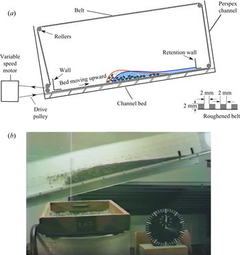


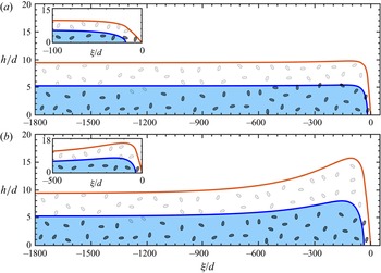


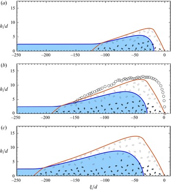


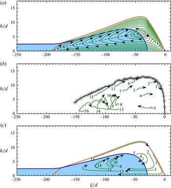


 Open access