


1 Introduction
Two- and three-dimensional bluff bodies in cross-flows are subjected to flow-induced, time-dependent loads that are commonly associated with shedding of vorticity concentrations into the near wake and may lead to unsteady motions. Examples include torsion-plunge-coupled flutter instability of aircraft wings (Fung Reference Fung1969), motion of high-aspect-ratio structures with bluff cross-sections (Parkinson Reference Parkinson1971), and cylindrical lines in marine oil exploration (Griffin & Ramberg Reference Griffin and Ramberg1982).
Oscillatory motions induced by time-periodic vortex shedding from high-aspect-ratio (nominally two-dimensional) cylinders in uniform flows, such that their major axes are normal to the flow direction, have been investigated extensively. These cylinders are usually supported at their spanwise edges by normal linear springs, and the ensuing body dynamics can be approximated as a forced second-order system. In one of the early investigations of such oscillation dynamics, Feng (Reference Feng1968) described a ‘lock-in’ mechanism by which vortex shedding close to the natural frequency of the cylinder–spring system couples to the cylinder’s natural oscillations, and the ensuing wake oscillations become locked to the cylinder’s natural frequency. In a later investigation, Blevins (Reference Blevins1990) showed that the lock-in can occur at Strouhal number
 $(St_{D})^{-1}\approx 5$
. The vortical structures in the wake of a cylinder in forced transverse oscillations were characterized by Williamson & Roshko (Reference Williamson and Roshko1988), who identified experimentally three dominant modes comprising trains of single (S) and pairs (P) of vortices – namely, 2S, 2P, and S
$(St_{D})^{-1}\approx 5$
. The vortical structures in the wake of a cylinder in forced transverse oscillations were characterized by Williamson & Roshko (Reference Williamson and Roshko1988), who identified experimentally three dominant modes comprising trains of single (S) and pairs (P) of vortices – namely, 2S, 2P, and S
 $+$
P. The transverse oscillations of a free cylinder (in the absence of springs, i.e.
$+$
P. The transverse oscillations of a free cylinder (in the absence of springs, i.e.
 $k=0$
, arguably more relevant to the present study) were investigated by Govardhan & Williamson (Reference Govardhan and Williamson2002), who showed the cylinder does not oscillate freely when its reduced mass
$k=0$
, arguably more relevant to the present study) were investigated by Govardhan & Williamson (Reference Govardhan and Williamson2002), who showed the cylinder does not oscillate freely when its reduced mass
 $m^{\ast }$
(the ratio of the cylinder’s mass to the mass of the displaced fluid) is above some critical value
$m^{\ast }$
(the ratio of the cylinder’s mass to the mass of the displaced fluid) is above some critical value
 $m_{c}^{\ast }$
. However, when
$m_{c}^{\ast }$
. However, when
 ${m^{\ast }<m}_{c}^{\ast }$
, the cylinder exhibits resonance which is independent of
${m^{\ast }<m}_{c}^{\ast }$
, the cylinder exhibits resonance which is independent of
 $St_{D}$
as long as it is sufficiently small, and the amplitude and frequency of oscillations depend only on
$St_{D}$
as long as it is sufficiently small, and the amplitude and frequency of oscillations depend only on
 $m^{\ast }$
. In a later review of flow-induced vibrations, Williamson & Govardhan (Reference Williamson and Govardhan2004) focused primarily on an elastically mounted cylinder in one degree of freedom, although they pointed to similarities among such motion and responses in two degrees of freedom, extending it to pivoted cylinders, and even tethered bodies. They noted that the regimes of induced vibrations depend on the physical characteristics of the model and on the spatial modes of the shed vortices. In particular, when
$m^{\ast }$
. In a later review of flow-induced vibrations, Williamson & Govardhan (Reference Williamson and Govardhan2004) focused primarily on an elastically mounted cylinder in one degree of freedom, although they pointed to similarities among such motion and responses in two degrees of freedom, extending it to pivoted cylinders, and even tethered bodies. They noted that the regimes of induced vibrations depend on the physical characteristics of the model and on the spatial modes of the shed vortices. In particular, when
 $m^{\ast }>m_{c}^{\ast }$
, the vibrations are within the lock-in regime of vortex shedding, indicating coupling to the near wake.
$m^{\ast }>m_{c}^{\ast }$
, the vibrations are within the lock-in regime of vortex shedding, indicating coupling to the near wake.
Flow-induced oscillations of cylinders have also been studied in multiple degrees of freedom. In an investigation of the motion of a cylinder pivoted at one end and oscillating in two degrees of freedom normal to a cross-flow (i.e. with axially varying oscillation amplitude), Flemming & Williamson (Reference Flemming and Williamson2005) demonstrated a connection between purely transverse motion and the transverse–streamwise response where the critical inertia in the two-dimensional (2D) motion was taken to be equivalent to the critical mass of the one-dimensional (1D) motion. Ryan et al. (Reference Ryan, Pregnalato, Thompson and Hourigan2004) and Carberry & Sheridan (Reference Carberry and Sheridan2007) used tethered cylinders in angular motion about a pivot point to investigate three-dimensional (3D) motions, and reported that lock in to shedding of 2S, 2P and P
 $+$
S vortex modes led to a range of complex, combined transverse/streamwise motions.
$+$
S vortex modes led to a range of complex, combined transverse/streamwise motions.
A 2D cylinder with a non-circular cross-section (for example, rectangular) can develop a flow-induced instability when a change in its attitude produces flow-induced loads that act to further increase this change. Such coupling can lead to large-amplitude oscillations of the cylindrical body (referred to as ‘galloping’) at frequencies that are usually much lower than the natural vortex shedding or wake frequencies but clearly affect the wake (Parkinson Reference Parkinson1989; Blevins Reference Blevins1990). Because of the disparity between the oscillation frequency of the cylinder and its natural shedding frequency, the dynamics of the galloping motion can be described using a quasisteady analysis in which the instantaneous flow-induced load is taken to be the same as the static force at the same attitude, such that there is effectively no phase delay between the body motion and the wake response.
Mitigation of flow-induced oscillations of moving bluff bodies has been traditionally attempted by disrupting the vortex shedding using passive devices, such as strakes, shrouds, fairings and plates, as discussed in detail in a review articles by Zdravkovich (Reference Zdravkovich1981) and Every, King & Weaver (Reference Every, King and Weaver1982). In recent years, there have been several efforts to apply open- and closed-loop control of flow-induced oscillations by independent spatial and temporal actuation. Chen et al. (Reference Chen, Xin, Xu, Li, Ou and Hu2013) demonstrated suppression of transverse oscillations of a spring-supported cylinder (Reynolds number
 $Re_{D}<150\,000$
,
$Re_{D}<150\,000$
,
 $m^{\ast }>1000$
) using four discrete suction holes across the span (azimuthally at
$m^{\ast }>1000$
) using four discrete suction holes across the span (azimuthally at
 $270^{\circ }$
relative to the cross-flow) and reported reduction in the drag and lift forces at some optimal suction rate. Other work by van Hout, Katz & Greenblatt (Reference van Hout, Katz and Greenblatt2013) used external acoustic actuation to mitigate the induced oscillations of tethered spheres of different
$270^{\circ }$
relative to the cross-flow) and reported reduction in the drag and lift forces at some optimal suction rate. Other work by van Hout, Katz & Greenblatt (Reference van Hout, Katz and Greenblatt2013) used external acoustic actuation to mitigate the induced oscillations of tethered spheres of different
 $m^{\ast }$
at relatively low Reynolds numbers (
$m^{\ast }$
at relatively low Reynolds numbers (
 $Re_{D}<3000$
) and showed that the actuation can either amplify or suppress the induced oscillations, ostensibly by coupling to the vortex shedding. Goyta, Mueller-Vahl & Greenblatt (Reference Goyta, Mueller-Vahl and Greenblatt2013) demonstrated the control effectiveness of plasma actuation of the flow off the leading edge of a tethered cube (
$Re_{D}<3000$
) and showed that the actuation can either amplify or suppress the induced oscillations, ostensibly by coupling to the vortex shedding. Goyta, Mueller-Vahl & Greenblatt (Reference Goyta, Mueller-Vahl and Greenblatt2013) demonstrated the control effectiveness of plasma actuation of the flow off the leading edge of a tethered cube (
 $m^{\ast }=65$
,
$m^{\ast }=65$
,
 $Re_{D}<50\,000$
), and reported that the actuation altered the pressure downstream of the actuation source by reducing the scale of the separation bubble.
$Re_{D}<50\,000$
), and reported that the actuation altered the pressure downstream of the actuation source by reducing the scale of the separation bubble.
The present wind tunnel investigations explore modification of the reciprocal coupling between a free axisymmetric cylindrical bluff body and its near wake for directional control by altering the near-wake flow and thereby the wake-induced loads. Controlled modifications of the near wake and, indirectly, of the flow-induced loads are effected by exploiting the receptivity of the aft-separating shear layer to weak fluidic actuation. In the present investigations, such control is demonstrated by modifying the attitude of a freely yawing axisymmetric bluff body about a pivot within its ogive forebody (in the absence of a torsional restoring force) such that the body’s axis of symmetry at rest is nominally aligned with the direction of the oncoming flow (
 $0.57\times 10^{5}<Re_{D}<2.3\times 10^{5}$
). In the absence of wake control, the body (
$0.57\times 10^{5}<Re_{D}<2.3\times 10^{5}$
). In the absence of wake control, the body (
 $m^{\ast }\sim 100$
) undergoes nominally time-periodic yaw oscillations whose characteristic frequency is over an order of magnitude lower than the vortex shedding frequency. The oscillations are sustained by balance between the lateral inertia and restoring flow loads over the body and clearly depend on its mass and inertia. It is noteworthy that this response bears some resemblance to transverse oscillations of a ‘free’ cylinder in the absence of spring support, albeit at a significantly lower
$m^{\ast }\sim 100$
) undergoes nominally time-periodic yaw oscillations whose characteristic frequency is over an order of magnitude lower than the vortex shedding frequency. The oscillations are sustained by balance between the lateral inertia and restoring flow loads over the body and clearly depend on its mass and inertia. It is noteworthy that this response bears some resemblance to transverse oscillations of a ‘free’ cylinder in the absence of spring support, albeit at a significantly lower
 $m^{\ast }$
(for example, Govardhan & Williamson (Reference Govardhan and Williamson2002) reported
$m^{\ast }$
(for example, Govardhan & Williamson (Reference Govardhan and Williamson2002) reported
 $m^{\ast }\sim 0.54$
compared to 100 in the present investigations). The limit-cycle oscillations of the axial bluff body bear some resemblance to the oscillations associated with the galloping instability discussed above (Parkinson Reference Parkinson1989). However, while in limit cycle of the galloping instability the net flow loads on the body are destabilizing (restoring loads are typically provided by the support mechanism), in the limit cycle of the present motion the net flow-induced loads are restoring (there is no need for external restoring loads).
$m^{\ast }\sim 0.54$
compared to 100 in the present investigations). The limit-cycle oscillations of the axial bluff body bear some resemblance to the oscillations associated with the galloping instability discussed above (Parkinson Reference Parkinson1989). However, while in limit cycle of the galloping instability the net flow loads on the body are destabilizing (restoring loads are typically provided by the support mechanism), in the limit cycle of the present motion the net flow-induced loads are restoring (there is no need for external restoring loads).
In the present investigations, the receptivity of the near wake to low-amplitude pulsed fluidic perturbations of azimuthal segments of the separating shear layer at its aft end is explored for manipulation of the base yaw oscillations. While by themselves these perturbations, which are applied using brief jet momentum pulses, cannot directly affect the body’s motion, earlier investigations using a static model (for example, Lambert, Vukasinovic & Glezer Reference Lambert, Vukasinovic and Glezer2015) demonstrated that exploiting the receptivity of the wake shear layer to these perturbations can yield bi-directional loads that are of comparable magnitude to the restoring loads during ‘free’ quasisteady yaw oscillations despite the significant disparity between the time scale of the body and the convective time scale. The present work explores how and to what extent the body dynamics can be altered, and whether perturbation of the wake can engender sufficient flow loads to stabilize or destabilize the motion and prescribe a desired, nominally stable attitude using closed-loop feedback control.
The paper is organized in four sections: the experimental set-up and procedures are described in § 2, the dynamics of the free bluff body model in the absence of actuation is analysed in § 3, the effects of transitory, pulsed synthetic jet actuation on the near wake and the body’s yaw attitude are discussed in § 4, and the effects of closed-loop flow control of the body’s attitude are presented in § 5. Concluding remarks are included in § 6 and the design of the closed-loop proportional integral derivative (PID) controller that alters the model dynamics is outlined in the Appendix.

Figure 1. Top (a), and aft (b) views of the wind tunnel axisymmetric model and the coordinate system, and corresponding magnified views of the orifice of one of the synthetic jet actuators (c,d). The two opposing actuators that are used in the present investigations are marked in (a) and (b).
2 Experimental set-up and procedures
The present investigations utilize an axisymmetric bluff body model (
 $c=165~\text{mm}$
long) that is geometrically similar to the model that was used in the earlier investigations of Lambert et al. (Reference Lambert, Vukasinovic and Glezer2015), as shown in figure 1(a,b). The model is constructed as a light-weight cylindrical shell fabricated using stereolithography and comprises a central round cylindrical segment with diameter
$c=165~\text{mm}$
long) that is geometrically similar to the model that was used in the earlier investigations of Lambert et al. (Reference Lambert, Vukasinovic and Glezer2015), as shown in figure 1(a,b). The model is constructed as a light-weight cylindrical shell fabricated using stereolithography and comprises a central round cylindrical segment with diameter
 $D=90~\text{mm}$
and length
$D=90~\text{mm}$
and length
 $L=90~\text{mm}$
, an upstream nose section having an elliptic forming curve that mates tangentially to the upstream edge of the cylindrical surface, and an aft end segment that is formed by an azimuthal Coanda surface with a constant radius
$L=90~\text{mm}$
, an upstream nose section having an elliptic forming curve that mates tangentially to the upstream edge of the cylindrical surface, and an aft end segment that is formed by an azimuthal Coanda surface with a constant radius
 $R_{C}=12.7~\text{mm}$
. The model’s near wake and flow-induced loads can be manipulated by two independently driven opposite synthetic jet actuators labelled Act1 and Act2 in figure 1(b) (synthetic jet actuators have been the subject of numerous studies, with their function in external flows shown in detail in a study by Glezer & Amitay (Reference Glezer and Amitay2002)). In order to prevent flow attachment to the curved surface in the absence of jet actuation, the azimuthal Coanda surface is offset radially relative to the main body by a backward-facing step (
$R_{C}=12.7~\text{mm}$
. The model’s near wake and flow-induced loads can be manipulated by two independently driven opposite synthetic jet actuators labelled Act1 and Act2 in figure 1(b) (synthetic jet actuators have been the subject of numerous studies, with their function in external flows shown in detail in a study by Glezer & Amitay (Reference Glezer and Amitay2002)). In order to prevent flow attachment to the curved surface in the absence of jet actuation, the azimuthal Coanda surface is offset radially relative to the main body by a backward-facing step (
 $h_{S}=1.5~\text{mm}$
high). Each jet is issued in the streamwise direction through an orifice (
$h_{S}=1.5~\text{mm}$
high). Each jet is issued in the streamwise direction through an orifice (
 $h_{J}=0.38~\text{mm}$
high, azimuthal arclength
$h_{J}=0.38~\text{mm}$
high, azimuthal arclength
 $34.3~\text{mm}$
,
$34.3~\text{mm}$
,
 $A_{J}=13.0~\text{mm}^{2}$
), as depicted in figure 1(c,d). The orifices of the two opposite actuators symmetrically intersect the model’s meridional (
$A_{J}=13.0~\text{mm}^{2}$
), as depicted in figure 1(c,d). The orifices of the two opposite actuators symmetrically intersect the model’s meridional (
 $x$
–
$x$
–
 $y$
) plane (i.e. the plane of yaw motion). The aft segment also contains a streamwise recess downstream of the orifice edge of each jet which bounds the jet azimuthally over a segmented arc (this geometry was optimized for recess height, orifice height and Coanda radius in studies by Rinehart (Reference Rinehart2011)). The mass of the assembled model with the actuators is 0.11 kg (
$y$
) plane (i.e. the plane of yaw motion). The aft segment also contains a streamwise recess downstream of the orifice edge of each jet which bounds the jet azimuthally over a segmented arc (this geometry was optimized for recess height, orifice height and Coanda radius in studies by Rinehart (Reference Rinehart2011)). The mass of the assembled model with the actuators is 0.11 kg (
 $m^{\ast }\sim 100$
). Jet actuation leads to the partial attachment of an azimuthal segment of the separating shear layer along the Coanda surface and turning of the outer flow into the wake, resulting in an aerodynamic reaction force that is normal to the jet’s centreline and an accompanying moment. In the present investigations, the maximum expulsion velocity of each jet is
$m^{\ast }\sim 100$
). Jet actuation leads to the partial attachment of an azimuthal segment of the separating shear layer along the Coanda surface and turning of the outer flow into the wake, resulting in an aerodynamic reaction force that is normal to the jet’s centreline and an accompanying moment. In the present investigations, the maximum expulsion velocity of each jet is
 $U_{J}=25~\text{m}~\text{s}^{-1}$
(the momentum coefficient
$U_{J}=25~\text{m}~\text{s}^{-1}$
(the momentum coefficient
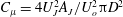 $C_{\unicode[STIX]{x1D707}}=4U_{J}^{2}A_{J}/U_{o}^{2}\unicode[STIX]{x03C0}D^{2}$
is
$C_{\unicode[STIX]{x1D707}}=4U_{J}^{2}A_{J}/U_{o}^{2}\unicode[STIX]{x03C0}D^{2}$
is
 $3.2\times 10^{-3}$
at
$3.2\times 10^{-3}$
at
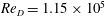
 $U_{o}=20~\text{m}~\text{s}^{-1},Re_{D}=1.15\times 10^{5}$
), at a fixed actuation frequency of 1.05 kHz (near resonance).
$U_{o}=20~\text{m}~\text{s}^{-1},Re_{D}=1.15\times 10^{5}$
), at a fixed actuation frequency of 1.05 kHz (near resonance).

Figure 2. Side (a) and rear (b) views of the wire-mounting mechanism of the free-yawing wind tunnel model and a view from upstream of the model mounted in the wind tunnel (c).
The model is wire-mounted in the wind tunnel’s
 $0.91\times 0.91$
m test section (free-stream speed
$0.91\times 0.91$
m test section (free-stream speed
 $U_{o}\leqslant 40~\text{m}~\text{s}^{-1}$
, turbulence level lower than 0.25 %) in a manner that enables nearly free yaw but restricts other motions. As shown in figure 2(a,b), the model is supported by a steel wire (1 mm diameter) that is thin enough so that its characteristic shedding frequency within the present free-stream speed range (
$U_{o}\leqslant 40~\text{m}~\text{s}^{-1}$
, turbulence level lower than 0.25 %) in a manner that enables nearly free yaw but restricts other motions. As shown in figure 2(a,b), the model is supported by a steel wire (1 mm diameter) that is thin enough so that its characteristic shedding frequency within the present free-stream speed range (
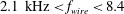 $2.1~\text{kHz}<f_{wire}<8.4$
kHz,
$2.1~\text{kHz}<f_{wire}<8.4$
kHz,
 $6.3\times 10^{2}<Re_{wire}<2.5\times 10^{3}$
) is decoupled from the nominal shedding frequency of the model (
$6.3\times 10^{2}<Re_{wire}<2.5\times 10^{3}$
) is decoupled from the nominal shedding frequency of the model (
 $27~\text{Hz}<f_{shed}<110~\text{Hz},5.7\times 10^{4}<Re_{D}<2.3\times 10^{5}$
). Each end of the mounting wire is secured to the tunnel’s wall through a vented screw (for tension adjustment) in a low-friction ball bearing that is attached to a wall-mounted shaft connector. The wire passes through the front end of the model and attaches to internal connectors. The yaw axis is placed at
$27~\text{Hz}<f_{shed}<110~\text{Hz},5.7\times 10^{4}<Re_{D}<2.3\times 10^{5}$
). Each end of the mounting wire is secured to the tunnel’s wall through a vented screw (for tension adjustment) in a low-friction ball bearing that is attached to a wall-mounted shaft connector. The wire passes through the front end of the model and attaches to internal connectors. The yaw axis is placed at
 $x_{o}=0.18c$
, upstream of the model’s static centre of pressure
$x_{o}=0.18c$
, upstream of the model’s static centre of pressure
 $x_{cp}\sim 0.33c$
, to realize semi-stable response (cf. § 3). Electrical connection to the actuators is provided by four ultrathin wires that are weaved through the tunnel walls along the support wire that serves as ground connection (the overall diameter is 1.5 mm). The model supported within the test section is shown in figure 2(c). The instantaneous attitude of the model’s centreline
$x_{cp}\sim 0.33c$
, to realize semi-stable response (cf. § 3). Electrical connection to the actuators is provided by four ultrathin wires that are weaved through the tunnel walls along the support wire that serves as ground connection (the overall diameter is 1.5 mm). The model supported within the test section is shown in figure 2(c). The instantaneous attitude of the model’s centreline
 $\unicode[STIX]{x1D6FC}_{z}$
relative to the streamwise (
$\unicode[STIX]{x1D6FC}_{z}$
relative to the streamwise (
 $x$
) direction is extracted from laser vibrometer measurements of the surface position at mid-body elevation,
$x$
) direction is extracted from laser vibrometer measurements of the surface position at mid-body elevation,
 $x_{L}=0.36c$
downstream of the mounting wire (when the model is aligned with the streamwise direction). The flow-induced vibration of the mounting wire was measured to have deflection and speed amplitudes of
$x_{L}=0.36c$
downstream of the mounting wire (when the model is aligned with the streamwise direction). The flow-induced vibration of the mounting wire was measured to have deflection and speed amplitudes of
 $\pm 0.16~\text{mm}$
and
$\pm 0.16~\text{mm}$
and
 $\pm 2~\text{mm}~\text{s}^{-1}$
, respectively. The estimated uncertainties of the model’s yawing angle and rate (
$\pm 2~\text{mm}~\text{s}^{-1}$
, respectively. The estimated uncertainties of the model’s yawing angle and rate (
 $\unicode[STIX]{x1D6FC}_{z}$
and
$\unicode[STIX]{x1D6FC}_{z}$
and
 $\dot{\unicode[STIX]{x1D6FC}_{z}}$
) owing to wire vibrations are
$\dot{\unicode[STIX]{x1D6FC}_{z}}$
) owing to wire vibrations are
 $0.3^{\circ }$
and
$0.3^{\circ }$
and
 $3.9\,^{\circ }\,\text{s}^{-1}$
, respectively.
$3.9\,^{\circ }\,\text{s}^{-1}$
, respectively.
The velocity field in the near wake of the model is measured in the
 $x$
–
$x$
–
 $y$
(yawing) plane using particle image velocimetry (PIV) acquired phase-locked to the yaw position of the model. The horizontal laser sheet plane is collinear with the model’s streamwise axis and the light is transmitted opposite to the laser vibrometer such that the model shields the PIV illumination from the vibrometer, and both measurements can be acquired simultaneously. The PIV field of view includes the aft end of the model and measures
$y$
(yawing) plane using particle image velocimetry (PIV) acquired phase-locked to the yaw position of the model. The horizontal laser sheet plane is collinear with the model’s streamwise axis and the light is transmitted opposite to the laser vibrometer such that the model shields the PIV illumination from the vibrometer, and both measurements can be acquired simultaneously. The PIV field of view includes the aft end of the model and measures
 $80~\text{mm}\times 160~\text{mm}$
with a flow field spatial resolution of 1.1 mm, resulting from the square PIV interrogation domain measuring 32 pixels on the side. The uncertainty of the phase-averaged velocity (using 170 realizations) based on root mean square (r.m.s.) fluctuations is estimated to be 3.2 %, and the corresponding uncertainty in the phase-averaged vorticity (velocity derivatives are calculated using a nine-point centred finite difference) is 8.2 %.
$80~\text{mm}\times 160~\text{mm}$
with a flow field spatial resolution of 1.1 mm, resulting from the square PIV interrogation domain measuring 32 pixels on the side. The uncertainty of the phase-averaged velocity (using 170 realizations) based on root mean square (r.m.s.) fluctuations is estimated to be 3.2 %, and the corresponding uncertainty in the phase-averaged vorticity (velocity derivatives are calculated using a nine-point centred finite difference) is 8.2 %.
3 The dynamic response of the free-yawing platform
The dynamic characteristics of the free-yawing body (cf. § 2) as a result of its interaction with the cross-flow are assessed from laser vibrometer measurements of its lateral motion over a range of wind tunnel speeds (
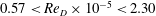 $0.57<Re_{D}\times 10^{-5}<2.30$
) that is bounded by the lowest stable tunnel speed and by the optical range of the vibrometer at large lateral yaw oscillations. As noted in § 1, the reciprocal coupling between the near wake and the motion of a bluff body results in unsteady flow-induced loads that, for the present model, drive nearly time-harmonic, lateral oscillatory motion. For example, at
$0.57<Re_{D}\times 10^{-5}<2.30$
) that is bounded by the lowest stable tunnel speed and by the optical range of the vibrometer at large lateral yaw oscillations. As noted in § 1, the reciprocal coupling between the near wake and the motion of a bluff body results in unsteady flow-induced loads that, for the present model, drive nearly time-harmonic, lateral oscillatory motion. For example, at
 $Re_{D}=1.15\times 10^{5}$
, the oscillation frequency is approximately 1.7 Hz, as depicted in the time history of the model’s attitude
$Re_{D}=1.15\times 10^{5}$
, the oscillation frequency is approximately 1.7 Hz, as depicted in the time history of the model’s attitude
 $\unicode[STIX]{x1D6FC}_{z}(t)$
and its power spectrum in figure 3(a,b), respectively (at this Reynolds number, the average amplitude of
$\unicode[STIX]{x1D6FC}_{z}(t)$
and its power spectrum in figure 3(a,b), respectively (at this Reynolds number, the average amplitude of
 $\unicode[STIX]{x1D6FC}_{z}(t)$
is
$\unicode[STIX]{x1D6FC}_{z}(t)$
is
 $6.9^{\circ }$
and its r.m.s. is
$6.9^{\circ }$
and its r.m.s. is
 $\tilde{\unicode[STIX]{x1D6FC}}_{z}\approx 4.8^{\circ }$
). That the characteristic oscillation frequency of the model is over two orders of magnitude lower than its shedding frequency (
$\tilde{\unicode[STIX]{x1D6FC}}_{z}\approx 4.8^{\circ }$
). That the characteristic oscillation frequency of the model is over two orders of magnitude lower than its shedding frequency (
 $St_{D}\approx 0.008$
and 0.2, respectively), and, similarly, its oscillation period is considerably longer than the convective time scale
$St_{D}\approx 0.008$
and 0.2, respectively), and, similarly, its oscillation period is considerably longer than the convective time scale
 $\unicode[STIX]{x1D70F}_{z}\approx 71\unicode[STIX]{x1D70F}_{conv}$
(
$\unicode[STIX]{x1D70F}_{z}\approx 71\unicode[STIX]{x1D70F}_{conv}$
(
 $\unicode[STIX]{x1D70F}_{conv}=c/U_{o}$
) indicates that the coupling between the near wake and the model occurs on global scales of the wake rather than the scales of the vortices in the aft-separating shear layer.
$\unicode[STIX]{x1D70F}_{conv}=c/U_{o}$
) indicates that the coupling between the near wake and the model occurs on global scales of the wake rather than the scales of the vortices in the aft-separating shear layer.

Figure 3. Time trace of an instantaneous model attitude
 $\unicode[STIX]{x1D6FC}_{z}(t)(Re_{D}=1.15\times 10^{5})$
(a), and its power spectrum (b), over twenty oscillation cycles.
$\unicode[STIX]{x1D6FC}_{z}(t)(Re_{D}=1.15\times 10^{5})$
(a), and its power spectrum (b), over twenty oscillation cycles.
The variation of the motion characteristics with
 $Re_{D}$
is shown in figure 4(a–c). These data show that the oscillations’ magnitude (as measured by
$Re_{D}$
is shown in figure 4(a–c). These data show that the oscillations’ magnitude (as measured by
 $\tilde{\unicode[STIX]{x1D6FC}}_{z}$
) and frequency,
$\tilde{\unicode[STIX]{x1D6FC}}_{z}$
) and frequency,
 $f_{z}$
, increase nearly linearly with
$f_{z}$
, increase nearly linearly with
 $Re_{D}$
(figures 4(a) and 4(b), respectively). However, while
$Re_{D}$
(figures 4(a) and 4(b), respectively). However, while
 $f_{z}$
increases monotonically with
$f_{z}$
increases monotonically with
 $Re_{D}$
, the ratio of the convective and lateral time scales,
$Re_{D}$
, the ratio of the convective and lateral time scales,
 $\unicode[STIX]{x1D70F}_{conv}/\unicode[STIX]{x1D70F}_{z}$
(figure 4
c), appears to have two distinct regimes. For
$\unicode[STIX]{x1D70F}_{conv}/\unicode[STIX]{x1D70F}_{z}$
(figure 4
c), appears to have two distinct regimes. For
 $Re_{D}<1.5\times 10^{5}$
, this ratio decreases monotonically with
$Re_{D}<1.5\times 10^{5}$
, this ratio decreases monotonically with
 $Re_{D}$
and reaches an nearly invariant level (approximately 0.013) when
$Re_{D}$
and reaches an nearly invariant level (approximately 0.013) when
 $Re_{D}>1.5\times 10^{5}$
. While the data in figure 4(b) shows that
$Re_{D}>1.5\times 10^{5}$
. While the data in figure 4(b) shows that
 $f_{z}$
is nearly linear with
$f_{z}$
is nearly linear with
 $Re_{D}$
within the range tested, this clearly does not imply a linear variation as
$Re_{D}$
within the range tested, this clearly does not imply a linear variation as
 $Re_{D}$
approaches zero. The linear fit within the present range intercepts the ordinate at some
$Re_{D}$
approaches zero. The linear fit within the present range intercepts the ordinate at some
 $f_{zo}>0$
, implying that
$f_{zo}>0$
, implying that
 $\unicode[STIX]{x1D70F}_{conv}/\unicode[STIX]{x1D70F}_{z}\sim C_{1}$
 $+C_{2}/U$
, where
$+C_{2}/U$
, where
 $C_{1}$
and
$C_{1}$
and
 $C_{2}$
are constants, resulting in the dependence
$C_{2}$
are constants, resulting in the dependence
 $\unicode[STIX]{x1D70F}_{conv}/\unicode[STIX]{x1D70F}_{z}\sim (U)^{-1}$
depicted in figure 4(c). This behaviour indicates that although the characteristic convective and oscillation time scales are still significantly disparate, they become ‘locked’ to multiples of each other as the flow speed increases, indicating stronger coupling between the aft-separating flow and the global model/wake dynamics.
$\unicode[STIX]{x1D70F}_{conv}/\unicode[STIX]{x1D70F}_{z}\sim (U)^{-1}$
depicted in figure 4(c). This behaviour indicates that although the characteristic convective and oscillation time scales are still significantly disparate, they become ‘locked’ to multiples of each other as the flow speed increases, indicating stronger coupling between the aft-separating flow and the global model/wake dynamics.

Figure 4. Variation with
 $Re_{D}$
of the r.m.s. attitude oscillations
$Re_{D}$
of the r.m.s. attitude oscillations
 $\tilde{\unicode[STIX]{x1D6FC}}_{z}$
(a), the model’s dominant lateral oscillation frequency
$\tilde{\unicode[STIX]{x1D6FC}}_{z}$
(a), the model’s dominant lateral oscillation frequency
 $f_{z}$
(b), and the ratio of the convective (streamwise) and lateral time scales
$f_{z}$
(b), and the ratio of the convective (streamwise) and lateral time scales
 $\unicode[STIX]{x1D70F}_{conv}/\unicode[STIX]{x1D70F}_{z}$
(c).
$\unicode[STIX]{x1D70F}_{conv}/\unicode[STIX]{x1D70F}_{z}$
(c).
Based on the quasiperiodic motion of the model, it is assumed that its dynamic response to the flow-induced loads can be described as a general second-order system:
 $$\begin{eqnarray}I\ddot{\unicode[STIX]{x1D6FC}_{z}}+C_{damp}\dot{\unicode[STIX]{x1D6FC}_{z}}+K\unicode[STIX]{x1D6FC}_{z}=M_{z}(t)\end{eqnarray}$$
and that its attitude (yaw angle) can be taken to be of the form
 $\unicode[STIX]{x1D6FC}_{z}(t)=A(t)\cos [\unicode[STIX]{x1D714}_{z}(t)\times t]$
. The coefficients
$\unicode[STIX]{x1D6FC}_{z}(t)=A(t)\cos [\unicode[STIX]{x1D714}_{z}(t)\times t]$
. The coefficients
 $I$
,
$I$
,
 $C_{damp}$
and
$C_{damp}$
and
 $K$
are the model’s inertia, damping and spring coefficients in the absence of the flow-induced loads (in the present system
$K$
are the model’s inertia, damping and spring coefficients in the absence of the flow-induced loads (in the present system
 $K=0$
). Assuming small angles of attack, the yawing angular motion of the model can be expressed as
$K=0$
). Assuming small angles of attack, the yawing angular motion of the model can be expressed as
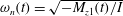
 $M_{z}(t)=M_{z1}(t)\unicode[STIX]{x1D6FC}_{z}+M_{z2}(t)\dot{\unicode[STIX]{x1D6FC}}_{z}$
, (for example, Bisplinghoff, Ashley & Halfman Reference Bisplinghoff, Ashley and Halfman1996). The motion of the model is then characterized in terms of the time-dependent natural frequency,
$M_{z}(t)=M_{z1}(t)\unicode[STIX]{x1D6FC}_{z}+M_{z2}(t)\dot{\unicode[STIX]{x1D6FC}}_{z}$
, (for example, Bisplinghoff, Ashley & Halfman Reference Bisplinghoff, Ashley and Halfman1996). The motion of the model is then characterized in terms of the time-dependent natural frequency,
 $\unicode[STIX]{x1D714}_{n}(t)$
, and damping ratio,
$\unicode[STIX]{x1D714}_{n}(t)$
, and damping ratio,
 $\unicode[STIX]{x1D709}(t)$
, as
$\unicode[STIX]{x1D709}(t)$
, as
 $$\begin{eqnarray}\ddot{\unicode[STIX]{x1D6FC}_{z}}+2\unicode[STIX]{x1D714}_{n}(t)\unicode[STIX]{x1D709}(t)\dot{\unicode[STIX]{x1D6FC}_{z}}+\unicode[STIX]{x1D714}_{n}^{2}(t)\unicode[STIX]{x1D6FC}_{z}=0.\end{eqnarray}$$
In this form
 $\unicode[STIX]{x1D714}_{n}(t)=\sqrt{-M_{z1}(t)/I}$
and
$\unicode[STIX]{x1D714}_{n}(t)=\sqrt{-M_{z1}(t)/I}$
and
 $\unicode[STIX]{x1D709}(t)=(C_{damp}-M_{z2}(t))/\sqrt{-IM_{z1}(t)}$
, which depend on both physical (
$\unicode[STIX]{x1D709}(t)=(C_{damp}-M_{z2}(t))/\sqrt{-IM_{z1}(t)}$
, which depend on both physical (
 $I$
,
$I$
,
 $C_{damp}$
) and aerodynamic properties [
$C_{damp}$
) and aerodynamic properties [
 $M_{z1}(t)$
and
$M_{z1}(t)$
and
 $M_{z2}(t)$
], and the aerodynamic force is restoring for harmonic oscillation [
$M_{z2}(t)$
], and the aerodynamic force is restoring for harmonic oscillation [
 $M_{z1}(t)<0$
]. The system’s inertia is estimated to be
$M_{z1}(t)<0$
]. The system’s inertia is estimated to be
 $I=7.9~\pm ~0.1\times 10^{-4}~\text{Nms}^{2}~\text{rad}^{-1}$
using the CAD design (neglecting the electrical wires). The model’s mechanical damping (caused by the wire and bearing mount) is estimated using a manual lateral impulse perturbation in the absence of external flow. The perturbation deflects the model from its centred position
$I=7.9~\pm ~0.1\times 10^{-4}~\text{Nms}^{2}~\text{rad}^{-1}$
using the CAD design (neglecting the electrical wires). The model’s mechanical damping (caused by the wire and bearing mount) is estimated using a manual lateral impulse perturbation in the absence of external flow. The perturbation deflects the model from its centred position
 $\unicode[STIX]{x1D6FC}_{z}\approx 0^{\circ }$
to
$\unicode[STIX]{x1D6FC}_{z}\approx 0^{\circ }$
to
 ${\approx}8^{\circ }$
(comparable to the lateral oscillation amplitude effected by the flow-induced loads in the presence of flow). The lateral time-dependent attitude of the model following the impulse is shown in figure 5, and the corresponding angular velocity and acceleration
${\approx}8^{\circ }$
(comparable to the lateral oscillation amplitude effected by the flow-induced loads in the presence of flow). The lateral time-dependent attitude of the model following the impulse is shown in figure 5, and the corresponding angular velocity and acceleration
 $\dot{\unicode[STIX]{x1D6FC}_{z}}(t)$
and
$\dot{\unicode[STIX]{x1D6FC}_{z}}(t)$
and
 $\ddot{\unicode[STIX]{x1D6FC}}_{z}(t)$
, respectively, are computed from these data. Using the second-order model, assuming
$\ddot{\unicode[STIX]{x1D6FC}}_{z}(t)$
, respectively, are computed from these data. Using the second-order model, assuming
 $M_{z}=0$
following the onset of the motion, the damping constant of the mounting system is estimated to be
$M_{z}=0$
following the onset of the motion, the damping constant of the mounting system is estimated to be
 $C_{damp}=1.20\pm 0.06\times 10^{-3}~\text{N}~\text{m}~\text{s}~\text{rad}^{-1}$
; the modelled motion is also shown in figure 5 and is in good agreement with the measured response.
$C_{damp}=1.20\pm 0.06\times 10^{-3}~\text{N}~\text{m}~\text{s}~\text{rad}^{-1}$
; the modelled motion is also shown in figure 5 and is in good agreement with the measured response.

Figure 5. Time traces of the motion of the one-degree-of-freedom model following an impulse yaw perturbation and the corresponding least squares fit to a mass–damper model are shown in blue and green traces, respectively.
The second-order formulation in (3.1) can be used to estimate the aerodynamic loads on the model in the presence of air flow. This approach is evaluated by considering the temporal variation of
 $\unicode[STIX]{x1D714}_{n}$
and
$\unicode[STIX]{x1D714}_{n}$
and
 $\unicode[STIX]{x1D709}$
when the lateral motion of the wind tunnel model commences from a stationary streamwise attitude. To this end, the model is held nearly stationary at a given tunnel speed using the actuation jets (as described in detail in § 5), followed by abruptly terminating the actuation. The ensuing time-dependent trajectory
$\unicode[STIX]{x1D709}$
when the lateral motion of the wind tunnel model commences from a stationary streamwise attitude. To this end, the model is held nearly stationary at a given tunnel speed using the actuation jets (as described in detail in § 5), followed by abruptly terminating the actuation. The ensuing time-dependent trajectory
 $\unicode[STIX]{x1D6FC}_{z}(t)$
of the model is measured phase-locked to the termination of the actuation as the model begins to oscillate laterally with increasing amplitude, until the nearly quasisteady limit-cycle amplitude is reached within approximately three oscillation cycles, as shown in figure 6(a). Also shown in figure 6(a) is a series of discrete model attitudes
$\unicode[STIX]{x1D6FC}_{z}(t)$
of the model is measured phase-locked to the termination of the actuation as the model begins to oscillate laterally with increasing amplitude, until the nearly quasisteady limit-cycle amplitude is reached within approximately three oscillation cycles, as shown in figure 6(a). Also shown in figure 6(a) is a series of discrete model attitudes
 $\unicode[STIX]{x1D6FC}_{z}^{i}$
at equally spaced time increments (0.2 s apart). The corresponding angular velocity and acceleration,
$\unicode[STIX]{x1D6FC}_{z}^{i}$
at equally spaced time increments (0.2 s apart). The corresponding angular velocity and acceleration,
 $\dot{\unicode[STIX]{x1D6FC}}_{z}^{i}$
and
$\dot{\unicode[STIX]{x1D6FC}}_{z}^{i}$
and
 $\ddot{\unicode[STIX]{x1D6FC}}_{z}^{i}$
, are evaluated at each time step, and
$\ddot{\unicode[STIX]{x1D6FC}}_{z}^{i}$
, are evaluated at each time step, and
 $\unicode[STIX]{x1D714}_{n}^{i}$
, and
$\unicode[STIX]{x1D714}_{n}^{i}$
, and
 $\unicode[STIX]{x1D709}^{i}$
are computed using a least squares fit to
$\unicode[STIX]{x1D709}^{i}$
are computed using a least squares fit to
 $\unicode[STIX]{x1D6FC}_{z}(t)$
within a time window
$\unicode[STIX]{x1D6FC}_{z}(t)$
within a time window
 $t-\unicode[STIX]{x0394}t<t<t+\unicode[STIX]{x0394}t$
(
$t-\unicode[STIX]{x0394}t<t<t+\unicode[STIX]{x0394}t$
(
 $\unicode[STIX]{x0394}t$
is taken to be 0.4 s or window width of
$\unicode[STIX]{x0394}t$
is taken to be 0.4 s or window width of
 $0.68\unicode[STIX]{x1D70F}_{z}$
where adjacent time windows are
$0.68\unicode[STIX]{x1D70F}_{z}$
where adjacent time windows are
 $0.34\unicode[STIX]{x1D70F}_{z}$
apart and have 75 % overlap). The resulting distributions of
$0.34\unicode[STIX]{x1D70F}_{z}$
apart and have 75 % overlap). The resulting distributions of
 $\unicode[STIX]{x1D714}_{n}^{i}$
, and
$\unicode[STIX]{x1D714}_{n}^{i}$
, and
 $\unicode[STIX]{x1D709}^{i}$
estimated at each time increment are shown in figure 6(b,c), respectively. Note that when the model is initially at equilibrium, its lateral motion starts due to stochastic vortex shedding, and the second-order model in (3.2) is probably inadequate to describe the initial motion (for this reason, the first time window is omitted). Each of figure 6(b,c) also includes exponential fits of the natural frequency and damping (
$\unicode[STIX]{x1D709}^{i}$
estimated at each time increment are shown in figure 6(b,c), respectively. Note that when the model is initially at equilibrium, its lateral motion starts due to stochastic vortex shedding, and the second-order model in (3.2) is probably inadequate to describe the initial motion (for this reason, the first time window is omitted). Each of figure 6(b,c) also includes exponential fits of the natural frequency and damping (
 $\unicode[STIX]{x1D714}_{n}(t)=10.74+4.67\text{e}^{-t/0.56}~\text{rad}~\text{s}^{-1}$
, and
$\unicode[STIX]{x1D714}_{n}(t)=10.74+4.67\text{e}^{-t/0.56}~\text{rad}~\text{s}^{-1}$
, and
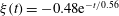 $\unicode[STIX]{x1D709}(t)=-0.48\text{e}^{-t/0.56}$
), where an exponential model with the same time constants is used for simplicity. These data show that the respective transitory magnitudes of the natural frequency and of the damping decrease and increase with time, and when the limit cycle of the natural oscillatory motion is reached, they attain nearly asymptotic levels (
$\unicode[STIX]{x1D709}(t)=-0.48\text{e}^{-t/0.56}$
), where an exponential model with the same time constants is used for simplicity. These data show that the respective transitory magnitudes of the natural frequency and of the damping decrease and increase with time, and when the limit cycle of the natural oscillatory motion is reached, they attain nearly asymptotic levels (
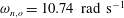 $\unicode[STIX]{x1D714}_{n,o}=10.74~\text{rad}~\text{s}^{-1}$
and
$\unicode[STIX]{x1D714}_{n,o}=10.74~\text{rad}~\text{s}^{-1}$
and
 $\unicode[STIX]{x1D709}_{o}\approx 0$
).
$\unicode[STIX]{x1D709}_{o}\approx 0$
).

Figure 6. Transitory variation of the model’s lateral oscillations from central rest attitude through its limit cycle: (a)
 $\unicode[STIX]{x1D6FC}_{z}(t)$
, where the magnitudes at equally spaced time increments are marked by (● (blue)); the corresponding natural frequency
$\unicode[STIX]{x1D6FC}_{z}(t)$
, where the magnitudes at equally spaced time increments are marked by (● (blue)); the corresponding natural frequency
 $\unicode[STIX]{x1D714}_{n}$
(b) and damping ratio,
$\unicode[STIX]{x1D714}_{n}$
(b) and damping ratio,
 $\unicode[STIX]{x1D709}$
(c) computed at each of the time increments in (a) along with an exponential fit; and (d) comparison of the resultant aerodynamic side force computed using the exponential fits to
$\unicode[STIX]{x1D709}$
(c) computed at each of the time increments in (a) along with an exponential fit; and (d) comparison of the resultant aerodynamic side force computed using the exponential fits to
 $\unicode[STIX]{x1D714}_{n}$
and
$\unicode[STIX]{x1D714}_{n}$
and
 $\unicode[STIX]{x1D709}$
with a previous measurements of the side force on a static model from Lambert et al. (Reference Lambert, Vukasinovic and Glezer2015) (●).
$\unicode[STIX]{x1D709}$
with a previous measurements of the side force on a static model from Lambert et al. (Reference Lambert, Vukasinovic and Glezer2015) (●).
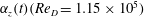
The fidelity of the model is first demonstrated by using it to estimate the static side force on the model at varying angles of attack which can be compared with earlier measurements on a static, geometrically similar model by Lambert et al. (Reference Lambert, Vukasinovic and Glezer2015). The natural frequency of the limit cycle is used to estimate the static sensitivity of the moment about the mounting wire:
 $$\begin{eqnarray}M_{z}|_{\dot{\unicode[STIX]{x1D6FC}_{z}}=0,t\rightarrow \infty }=M_{z1}|_{t\rightarrow \infty }\unicode[STIX]{x1D6FC}_{z}=-I\unicode[STIX]{x1D714}_{n,o}^{2}\unicode[STIX]{x1D6FC}_{z},\end{eqnarray}$$
which is then used to approximate the corresponding side force from a moment balance about the model’s centre of pressure (where the aerodynamic moment vanishes):
 $$\begin{eqnarray}F_{y}|_{\dot{\unicode[STIX]{x1D6FC}_{z}}=0,t\rightarrow \infty }=\frac{M_{z}|_{\dot{\unicode[STIX]{x1D6FC}_{z}}=0,t\rightarrow \infty }}{x_{0}-x_{cp}}=\frac{I\unicode[STIX]{x1D714}_{n,o}^{2}\unicode[STIX]{x1D6FC}_{z}}{0.15c},\end{eqnarray}$$
where
 $x_{o}$
and
$x_{o}$
and
 $x_{cp}$
are the respective streamwise positions of the model’s centre of lateral oscillation and its centre of pressure. This predicted aerodynamic side force (plotted as the side force coefficient
$x_{cp}$
are the respective streamwise positions of the model’s centre of lateral oscillation and its centre of pressure. This predicted aerodynamic side force (plotted as the side force coefficient
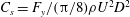 $C_{s}=F_{y}/(\unicode[STIX]{x03C0}/8)\unicode[STIX]{x1D70C}U^{2}D^{2}$
, where
$C_{s}=F_{y}/(\unicode[STIX]{x03C0}/8)\unicode[STIX]{x1D70C}U^{2}D^{2}$
, where
 $\unicode[STIX]{x1D70C}$
is fluid density) is shown in figure 6(d) and plotted with the earlier measurements of Lambert et al. (Reference Lambert, Vukasinovic and Glezer2015), and shows good agreement. This agreement suggests that the oscillation frequency of the model’s primary limit cycle about another centre of rotation upstream of the centre of pressure can, in principle, be estimated from measurements of the static aerodynamic force.
$\unicode[STIX]{x1D70C}$
is fluid density) is shown in figure 6(d) and plotted with the earlier measurements of Lambert et al. (Reference Lambert, Vukasinovic and Glezer2015), and shows good agreement. This agreement suggests that the oscillation frequency of the model’s primary limit cycle about another centre of rotation upstream of the centre of pressure can, in principle, be estimated from measurements of the static aerodynamic force.
The predicted
 $\unicode[STIX]{x1D714}_{n}(t)$
and
$\unicode[STIX]{x1D714}_{n}(t)$
and
 $\unicode[STIX]{x1D709}(t)$
are further validated by comparing the predictions of
$\unicode[STIX]{x1D709}(t)$
are further validated by comparing the predictions of
 $\unicode[STIX]{x1D6FC}_{z}(t)$
and angular velocity
$\unicode[STIX]{x1D6FC}_{z}(t)$
and angular velocity
 $\dot{\unicode[STIX]{x1D6FC}_{z}}(t)$
with the experimental measurements (this is a demonstration of how well the model’s
$\dot{\unicode[STIX]{x1D6FC}_{z}}(t)$
with the experimental measurements (this is a demonstration of how well the model’s
 $\unicode[STIX]{x1D714}_{n}$
and
$\unicode[STIX]{x1D714}_{n}$
and
 $\unicode[STIX]{x1D709}$
fit the experimental data). To do this, the second-order model of the system (cf. (3.2)) is rewritten as a discrete time equation using a forward Euler update rule:
$\unicode[STIX]{x1D709}$
fit the experimental data). To do this, the second-order model of the system (cf. (3.2)) is rewritten as a discrete time equation using a forward Euler update rule:
 $$\begin{eqnarray}\left.\left[\begin{array}{@{}c@{}}\dot{\unicode[STIX]{x1D6FC}_{z}}\\ \ddot{\unicode[STIX]{x1D6FC}_{z}}\end{array}\right]\right|_{t}=\left[\begin{array}{@{}cc@{}}0 & 1\\ -\unicode[STIX]{x1D714}_{n}^{2} & -2\unicode[STIX]{x1D714}_{n}\unicode[STIX]{x1D709}\\ \end{array}\right]\left.\left[\begin{array}{@{}c@{}}\unicode[STIX]{x1D6FC}_{z}\\ \dot{\unicode[STIX]{x1D6FC}_{z}}\end{array}\right]\right|_{t}\quad \left.\left[\begin{array}{@{}c@{}}\unicode[STIX]{x1D6FC}_{z}\\ \dot{\unicode[STIX]{x1D6FC}_{z}}\end{array}\right]\right|_{t+1}=\left.\left[\begin{array}{@{}c@{}}\unicode[STIX]{x1D6FC}_{z}\\ \dot{\unicode[STIX]{x1D6FC}_{z}}\end{array}\right]\right|_{t}+\left.\left[\begin{array}{@{}c@{}}\dot{\unicode[STIX]{x1D6FC}_{z}}\\ \ddot{\unicode[STIX]{x1D6FC}_{z}}\end{array}\right]\right|_{t}\unicode[STIX]{x0394}t,\end{eqnarray}$$
which yields
 $\unicode[STIX]{x1D6FC}_{z}(t)$
,
$\unicode[STIX]{x1D6FC}_{z}(t)$
,
 $\dot{\unicode[STIX]{x1D6FC}_{z}}(t)$
and
$\dot{\unicode[STIX]{x1D6FC}_{z}}(t)$
and
 $\ddot{\unicode[STIX]{x1D6FC}_{z}}(t)$
given
$\ddot{\unicode[STIX]{x1D6FC}_{z}}(t)$
given
 $\unicode[STIX]{x1D714}_{n}$
(
$\unicode[STIX]{x1D714}_{n}$
(
 $t$
) and
$t$
) and
 $\unicode[STIX]{x1D709}$
(
$\unicode[STIX]{x1D709}$
(
 $t$
) and initial conditions (
$t$
) and initial conditions (
 $\unicode[STIX]{x1D6FC}_{z}|_{t=0}$
and
$\unicode[STIX]{x1D6FC}_{z}|_{t=0}$
and
 $\dot{\unicode[STIX]{x1D6FC}_{z}}|_{t=0}$
).
$\dot{\unicode[STIX]{x1D6FC}_{z}}|_{t=0}$
).
Note that since the initial attitude of the model
 $\unicode[STIX]{x1D6FC}_{z}|_{t=0}$
is nominally set by flow control actuation, the initial conditions are estimated at rest (
$\unicode[STIX]{x1D6FC}_{z}|_{t=0}$
is nominally set by flow control actuation, the initial conditions are estimated at rest (
 $\dot{\unicode[STIX]{x1D6FC}_{z}}|_{t=0}=0$
) with an initial attitude selected to minimize deviations between the predicted and measured trajectories (
$\dot{\unicode[STIX]{x1D6FC}_{z}}|_{t=0}=0$
) with an initial attitude selected to minimize deviations between the predicted and measured trajectories (
 $\dot{\unicode[STIX]{x1D6FC}}_{z}|_{t=0}=0.15^{\circ }$
). Figure 7(a,b) demonstrates a very good agreement between the time-dependent measured and predicted trajectories using the computed
$\dot{\unicode[STIX]{x1D6FC}}_{z}|_{t=0}=0.15^{\circ }$
). Figure 7(a,b) demonstrates a very good agreement between the time-dependent measured and predicted trajectories using the computed
 $\unicode[STIX]{x1D714}_{n}(t)$
and
$\unicode[STIX]{x1D714}_{n}(t)$
and
 $\unicode[STIX]{x1D709}(t)$
. The measured
$\unicode[STIX]{x1D709}(t)$
. The measured
 $\dot{\unicode[STIX]{x1D6FC}_{z}}$
in figure 7(b) shows the presence of a secondary, higher-frequency band (around
$\dot{\unicode[STIX]{x1D6FC}_{z}}$
in figure 7(b) shows the presence of a secondary, higher-frequency band (around
 $St_{D}=0.081$
) in the time derivative of the measured model response which is not captured by the prediction (it is also noticeable in the model’s attitude in figure 7
a). This secondary frequency is attributed to aerodynamic oscillations of the support wire that are triggered by aerodynamic impulse perturbation when the model is released from rest, and it diminishes significantly as the model approaches its limit cycle (
$St_{D}=0.081$
) in the time derivative of the measured model response which is not captured by the prediction (it is also noticeable in the model’s attitude in figure 7
a). This secondary frequency is attributed to aerodynamic oscillations of the support wire that are triggered by aerodynamic impulse perturbation when the model is released from rest, and it diminishes significantly as the model approaches its limit cycle (
 $2\unicode[STIX]{x1D70F}_{z}$
or
$2\unicode[STIX]{x1D70F}_{z}$
or
 $t>150\unicode[STIX]{x1D70F}_{conv}$
). Finally, the predicted moment coefficient of
$t>150\unicode[STIX]{x1D70F}_{conv}$
). Finally, the predicted moment coefficient of
 $M_{z}$
,
$M_{z}$
,
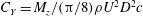 $C_{Y}=M_{z}/(\unicode[STIX]{x03C0}/8)\unicode[STIX]{x1D70C}U^{2}D^{2}c$
following the release of the model is computed from measurements of
$C_{Y}=M_{z}/(\unicode[STIX]{x03C0}/8)\unicode[STIX]{x1D70C}U^{2}D^{2}c$
following the release of the model is computed from measurements of
 $\unicode[STIX]{x1D6FC}_{z}(t)$
and
$\unicode[STIX]{x1D6FC}_{z}(t)$
and
 $\dot{\unicode[STIX]{x1D6FC}}_{z}(t)$
using the second-order model, and is shown in a phase plot with respect to
$\dot{\unicode[STIX]{x1D6FC}}_{z}(t)$
using the second-order model, and is shown in a phase plot with respect to
 $\unicode[STIX]{x1D6FC}_{z}$
in figure 7(c). The phase plot of
$\unicode[STIX]{x1D6FC}_{z}$
in figure 7(c). The phase plot of
 $C_{Y}$
shows the monotonic increase in the amplitude of the moment and hysteresis following the release of the model. As the limit cycle is approached, the moment distribution exhibits peaks as the model reaches each of its maximum attitude excursions before it changes the motion direction. These peaks are associated with vortex shedding that appears to be akin to dynamic stall of a pitching airfoil beyond its stall margin (for example, Rival & Tropea Reference Rival and Tropea2010). Similar phase plots are used in §§ 5 and 6 to characterize the respective state transition of the model dynamics with open- and closed-loop actuation.
$C_{Y}$
shows the monotonic increase in the amplitude of the moment and hysteresis following the release of the model. As the limit cycle is approached, the moment distribution exhibits peaks as the model reaches each of its maximum attitude excursions before it changes the motion direction. These peaks are associated with vortex shedding that appears to be akin to dynamic stall of a pitching airfoil beyond its stall margin (for example, Rival & Tropea Reference Rival and Tropea2010). Similar phase plots are used in §§ 5 and 6 to characterize the respective state transition of the model dynamics with open- and closed-loop actuation.

Figure 7. Time traces of measured (black) and predicted (green) model yaw attitude trajectories
 $\unicode[STIX]{x1D6FC}_{z}$
(a), and
$\unicode[STIX]{x1D6FC}_{z}$
(a), and
 $\dot{\unicode[STIX]{x1D6FC}_{z}}$
(b). The corresponding phase plot of
$\dot{\unicode[STIX]{x1D6FC}_{z}}$
(b). The corresponding phase plot of
 $C_{Y}$
versus
$C_{Y}$
versus
 $\unicode[STIX]{x1D6FC}_{z}$
is shown in (c).
$\unicode[STIX]{x1D6FC}_{z}$
is shown in (c).
The structure of the model’s near wake during its free yaw oscillations (in the absence of actuation) are captured using phase-locked PIV measurements in the horizontal
 $x$
–
$x$
–
 $y$
centre (meridional) plane during a complete (phase-averaged) oscillation cycle (the average oscillation period at
$y$
centre (meridional) plane during a complete (phase-averaged) oscillation cycle (the average oscillation period at
 $Re_{D~}=1.15\times 10^{5}$
is
$Re_{D~}=1.15\times 10^{5}$
is
 $\unicode[STIX]{x1D70F}_{z}=0.575~\text{s}$
). The PIV measurement domain is
$\unicode[STIX]{x1D70F}_{z}=0.575~\text{s}$
). The PIV measurement domain is
 $1.3<x/D<2.2$
and
$1.3<x/D<2.2$
and
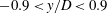 $-0.9<y/D<0.9$
(
$-0.9<y/D<0.9$
(
 $x=y=0$
is the position of the mounting wire). These PIV data are acquired at a fixed rate (7.8 Hz), and are sorted into 28 ‘bins’ of equally spaced yaw angles during the nominally time-periodic lateral oscillations such that, at each yaw angle, the phase-averaged velocity field is computed using 170 realizations. Eight realizations at (approximately) equal time increments during a single oscillation cycle are shown in figure 8.
$x=y=0$
is the position of the mounting wire). These PIV data are acquired at a fixed rate (7.8 Hz), and are sorted into 28 ‘bins’ of equally spaced yaw angles during the nominally time-periodic lateral oscillations such that, at each yaw angle, the phase-averaged velocity field is computed using 170 realizations. Eight realizations at (approximately) equal time increments during a single oscillation cycle are shown in figure 8.

Figure 8. Colour raster plots of concentrations of phase-averaged streamwise (
 $\hat{u}$
, a) and cross-stream (
$\hat{u}$
, a) and cross-stream (
 $\hat{v}$
, b) velocity components and of the azimuthal vorticity (
$\hat{v}$
, b) velocity components and of the azimuthal vorticity (
 $\hat{\unicode[STIX]{x1D701}}$
, c), in the near wake during the oscillation cycle (
$\hat{\unicode[STIX]{x1D701}}$
, c), in the near wake during the oscillation cycle (
 $0<t/\unicode[STIX]{x1D70F}_{z}<0.875$
, at equal increments
$0<t/\unicode[STIX]{x1D70F}_{z}<0.875$
, at equal increments
 $0.125\unicode[STIX]{x1D70F}_{z}$
,
$0.125\unicode[STIX]{x1D70F}_{z}$
,
 $Re_{D}=1.15\times 10^{5}$
).
$Re_{D}=1.15\times 10^{5}$
).
The flow measurements in the meridional (
 $x$
–
$x$
–
 $y$
) plane demonstrate that the near wake is dominated by partial, time-periodic attachment to azimuthal segments of the Coanda surface at the aft section of the model normal to the measurement plane (Lambert et al.
Reference Lambert, Vukasinovic and Glezer2015). As the model moves, the near wake becomes laterally distorted in concert with the yaw oscillations as the wake is deflected in a direction that is opposite to the sense of rotation, commensurate with the alternating flow-induced side forces on the model (note that the near wake is nominally symmetric about the meridional plane). Figure 8(a–c) shows a sequence of colour raster plots of concentrations of phase-averaged streamwise and cross-stream velocity components
$y$
) plane demonstrate that the near wake is dominated by partial, time-periodic attachment to azimuthal segments of the Coanda surface at the aft section of the model normal to the measurement plane (Lambert et al.
Reference Lambert, Vukasinovic and Glezer2015). As the model moves, the near wake becomes laterally distorted in concert with the yaw oscillations as the wake is deflected in a direction that is opposite to the sense of rotation, commensurate with the alternating flow-induced side forces on the model (note that the near wake is nominally symmetric about the meridional plane). Figure 8(a–c) shows a sequence of colour raster plots of concentrations of phase-averaged streamwise and cross-stream velocity components
 $\hat{u} (t)$
and
$\hat{u} (t)$
and
 $\hat{v}(t)$
, respectively, and of the azimuthal vorticity
$\hat{v}(t)$
, respectively, and of the azimuthal vorticity
 $\hat{\unicode[STIX]{x1D701}}(t)$
during the oscillation cycle (
$\hat{\unicode[STIX]{x1D701}}(t)$
during the oscillation cycle (
 $0<t/\unicode[STIX]{x1D70F}_{z}<0.875$
, at increments of
$0<t/\unicode[STIX]{x1D70F}_{z}<0.875$
, at increments of
 $0.125\unicode[STIX]{x1D70F}_{z}$
). The aft end of the body and its attitude are also shown for reference in each raster plot.
$0.125\unicode[STIX]{x1D70F}_{z}$
). The aft end of the body and its attitude are also shown for reference in each raster plot.
The streamwise velocity distributions within the meridional plane (figure 8
a) exhibit a clear reversed flow domain within a local ‘bubble’ that is bounded by a counter-current separating shear layer on each cross-stream end. The reversed streamwise velocity has a clear, transversely oscillating local maximum that diminishes towards the edges of the bubble. The offset of this maximum relative to the model’s centreline, when the latter is aligned with the direction of the tunnel’s flow at
 $t/\unicode[STIX]{x1D70F}_{z}=0$
and 0.5 (
$t/\unicode[STIX]{x1D70F}_{z}=0$
and 0.5 (
 $y/D=\pm 0.075$
,
$y/D=\pm 0.075$
,
 $x/D=1.9$
), is indicative of the inherent flow latency relative to the motion of the model, that ostensibly contributes to aerodynamic damping of the motion. The transverse asymmetry of the flow during the oscillation cycle is also evident by alternating attachment to the aft Coanda surface (nominally on opposite sides of the model’s centreline relative to the position of its front stagnation point). This attachment is accompanied by significant cross-stream flow, as demonstrated in figure 8(b3,7), which accentuates the asymmetry of the near wake near the transverse extremes of the model’s motion. The residual asymmetry at the midpoints of the oscillation cycle (figure 8
b1,5) is another indication of the latency in the wake flow. While the asymmetry of the opposite, separating shear layer segments at the midpoints of the oscillation cycle (figure 8
c1,5) is somewhat less pronounced, the partial attachment of these shear layer segments to the aft Coanda surface (figure 8
c3,7) results in strong flow deflection into the near wake that is coupled to the attitude of the model. During the peak of these opposite deflections, the internal vorticity concentrations within the near-wake bubble are of the same sense as the corresponding deflecting shear layer segment. This deflection is accompanied by strong cross-stream velocity (cf. figure 8
b3,7), indicating entrainment of the cross-flow into the near wake, although this entrainment does not significantly diminish the reversed flow within the wake (cf. figure 8
a3,7), nor does it lead to pronounced changes in the spreading of the separating shear layer at the cross-stream edges of the near-wake bubble. In fact, as shown by Sarioglu, Akansu & Yavuz (Reference Sarioglu, Akansu and Yavuz2005), the characteristic frequency of the separating shear layer, shedding off a streamwise cylinder model with an aspect ratio
$x/D=1.9$
), is indicative of the inherent flow latency relative to the motion of the model, that ostensibly contributes to aerodynamic damping of the motion. The transverse asymmetry of the flow during the oscillation cycle is also evident by alternating attachment to the aft Coanda surface (nominally on opposite sides of the model’s centreline relative to the position of its front stagnation point). This attachment is accompanied by significant cross-stream flow, as demonstrated in figure 8(b3,7), which accentuates the asymmetry of the near wake near the transverse extremes of the model’s motion. The residual asymmetry at the midpoints of the oscillation cycle (figure 8
b1,5) is another indication of the latency in the wake flow. While the asymmetry of the opposite, separating shear layer segments at the midpoints of the oscillation cycle (figure 8
c1,5) is somewhat less pronounced, the partial attachment of these shear layer segments to the aft Coanda surface (figure 8
c3,7) results in strong flow deflection into the near wake that is coupled to the attitude of the model. During the peak of these opposite deflections, the internal vorticity concentrations within the near-wake bubble are of the same sense as the corresponding deflecting shear layer segment. This deflection is accompanied by strong cross-stream velocity (cf. figure 8
b3,7), indicating entrainment of the cross-flow into the near wake, although this entrainment does not significantly diminish the reversed flow within the wake (cf. figure 8
a3,7), nor does it lead to pronounced changes in the spreading of the separating shear layer at the cross-stream edges of the near-wake bubble. In fact, as shown by Sarioglu, Akansu & Yavuz (Reference Sarioglu, Akansu and Yavuz2005), the characteristic frequency of the separating shear layer, shedding off a streamwise cylinder model with an aspect ratio
 $L/D=2$
and flat front and rear end surfaces (
$L/D=2$
and flat front and rear end surfaces (
 $Re_{D}=3.4\times 10^{4}$
), is nearly invariant with its attitude (these authors reported that the shedding frequency typically decreased with increasing
$Re_{D}=3.4\times 10^{4}$
), is nearly invariant with its attitude (these authors reported that the shedding frequency typically decreased with increasing
 $L/D$
).
$L/D$
).
Following the procedure of Ploumhans et al. (Reference Ploumhans, Winckelmans, Salmon, Leonard and Warren2002), the velocity measurements in the near wake can be used to estimate the induced aerodynamic moment on the model. Such an estimate is useful for identifying the coupling between the wake and the model’s motion, and is also used in § 5 to evaluate the flow control efficacy. These authors used a control volume that encompasses the flow surrounding a body in a uniform stream to calculate the force
 $\boldsymbol{F}$
exerted on the body based on the vortex impulses
$\boldsymbol{F}$
exerted on the body based on the vortex impulses
 $\boldsymbol{I}$
in its wake:
$\boldsymbol{I}$
in its wake:
where
 $\boldsymbol{r}$
is the distance of a fluid particle in the wake from a fixed origin which, in the present experiments, is taken to be the axis of the mounting wire, and the flow is assumed to be incompressible. This formulation can be extended to account for the aerodynamic moment about the mounting wire of the present model:
$\boldsymbol{r}$
is the distance of a fluid particle in the wake from a fixed origin which, in the present experiments, is taken to be the axis of the mounting wire, and the flow is assumed to be incompressible. This formulation can be extended to account for the aerodynamic moment about the mounting wire of the present model:

Since the phase-averaged flow is taken to be symmetric about the meridional (
 $x$
–
$x$
–
 $y$
) plane, it is argued that the vertical velocity and the non-azimuthal vorticity components vanish in this plane (
$y$
) plane, it is argued that the vertical velocity and the non-azimuthal vorticity components vanish in this plane (
 $\unicode[STIX]{x1D701}_{x}=\unicode[STIX]{x1D701}_{y}=0$
,
$\unicode[STIX]{x1D701}_{x}=\unicode[STIX]{x1D701}_{y}=0$
,
 $w=0$
,
$w=0$
,
 $\unicode[STIX]{x1D701}_{z}=\hat{\unicode[STIX]{x1D701}}$
), which reduces the contribution to the moment from the flow in the meridional plane to:
$\unicode[STIX]{x1D701}_{z}=\hat{\unicode[STIX]{x1D701}}$
), which reduces the contribution to the moment from the flow in the meridional plane to:
 $$\begin{eqnarray}\text{d}\hat{M}_{z}|_{z=0}=\iint \frac{\unicode[STIX]{x1D70C}}{2}(\dot{\hat{\unicode[STIX]{x1D701}}}(r_{x}^{2}+r_{y}^{2})+\hat{\unicode[STIX]{x1D701}}(r_{x}\hat{u} +r_{y}\hat{v}))\,\text{d}y\,\text{d}x=\iint \text{d}\hat{M}_{xyz}\,\text{d}y\,\text{d}x=\int \text{d}\hat{M}_{xz}\,\text{d}x.\end{eqnarray}$$
Although the present measurements do not encompass the entire streamwise extent of the wake, the measurements in the meridional plane within the near-wake domain shown in figure 8 yield some useful indication of the wake contribution to the aerodynamic yawing moment through the integrands of (3.8),
 $\text{d}\hat{M}_{xyz}(x,y,t)$
, and
$\text{d}\hat{M}_{xyz}(x,y,t)$
, and
 $\text{d}\hat{M}_{xz}(x,t)$
. The time rate of change of the measured azimuthal vorticity,
$\text{d}\hat{M}_{xz}(x,t)$
. The time rate of change of the measured azimuthal vorticity,
 $\dot{\hat{\unicode[STIX]{x1D701}}}$
, was estimated using the 28 measured phases during the wake oscillation, and the contribution from the unsteady term,
$\dot{\hat{\unicode[STIX]{x1D701}}}$
, was estimated using the 28 measured phases during the wake oscillation, and the contribution from the unsteady term,
 $\dot{\hat{\unicode[STIX]{x1D701}}}(r_{x}^{2}+r_{y}^{2})$
, is an order of magnitude smaller than the steady term,
$\dot{\hat{\unicode[STIX]{x1D701}}}(r_{x}^{2}+r_{y}^{2})$
, is an order of magnitude smaller than the steady term,
 $\hat{\unicode[STIX]{x1D701}}(r_{x}\hat{u} +r_{y}\hat{v})$
, indicating the absence of large unsteady aerodynamic effects.
$\hat{\unicode[STIX]{x1D701}}(r_{x}\hat{u} +r_{y}\hat{v})$
, indicating the absence of large unsteady aerodynamic effects.

Figure 9. Colour raster plots of
 $\text{d}\hat{M}_{xyz}$
(
$\text{d}\hat{M}_{xyz}$
(
 $y,t|x=\text{const.}$
) in the meridional
$y,t|x=\text{const.}$
) in the meridional
 $x$
–
$x$
–
 $y$
measurement domain (cf. figure 8) at
$y$
measurement domain (cf. figure 8) at
 $x/D=1.8$
(a), and 2.05 (b); the variation of
$x/D=1.8$
(a), and 2.05 (b); the variation of
 $\text{d}\hat{M}_{xz}$
(
$\text{d}\hat{M}_{xz}$
(
 $x$
,
$x$
,
 $t$
) during the base lateral oscillation cycle is shown in (c).
$t$
) during the base lateral oscillation cycle is shown in (c).
Figure 9(a–c) shows colour raster plots of
 $\text{d}\hat{M}_{xyz}$
(
$\text{d}\hat{M}_{xyz}$
(
 $x$
,
$x$
,
 $y$
,
$y$
,
 $t$
) during the lateral oscillation cycle. Figure 9(a,b) shows
$t$
) during the lateral oscillation cycle. Figure 9(a,b) shows
 $\text{d}\hat{M}_{xyz}$
(
$\text{d}\hat{M}_{xyz}$
(
 $y$
,
$y$
,
 $t$
;
$t$
;
 $x=\text{const.}$
) for two representative streamwise positions,
$x=\text{const.}$
) for two representative streamwise positions,
 $x/D=1.8$
and 2.05, while in figure 9(c),
$x/D=1.8$
and 2.05, while in figure 9(c),
 $\text{d}\hat{M}_{xyz}$
is integrated in
$\text{d}\hat{M}_{xyz}$
is integrated in
 $y$
(across the wake) to yield a map of
$y$
(across the wake) to yield a map of
 $\text{d}\hat{M}_{xz}(x,t)$
within the domain
$\text{d}\hat{M}_{xz}(x,t)$
within the domain
 $1.3<x/D<2.2$
. The data in figure 9(a) show that the contributions to the induced moment at
$1.3<x/D<2.2$
. The data in figure 9(a) show that the contributions to the induced moment at
 $x/D=1.8$
downstream of the model come from the vorticity concentrations within the separating shear layers that undulate along the
$x/D=1.8$
downstream of the model come from the vorticity concentrations within the separating shear layers that undulate along the
 $y$
axis during the lateral oscillations of the model, where the contribution of the opposite shear layer segments are nearly equal. This is also shown in figure 9(c), where the vorticity concentrations integrated in the cross-stream (
$y$
axis during the lateral oscillations of the model, where the contribution of the opposite shear layer segments are nearly equal. This is also shown in figure 9(c), where the vorticity concentrations integrated in the cross-stream (
 $y$
) direction lead to small net contributions to the model moment at
$y$
) direction lead to small net contributions to the model moment at
 $x/D=1.8$
. However, at
$x/D=1.8$
. However, at
 $x/D=2.05$
in figure 9(b), these contributions alternately intensify as the model reaches each lateral extreme (as the weaker layer rolls up to a large-scale vortex in figure 8
c3,7). This is in concert with the data in figure 9(c) for
$x/D=2.05$
in figure 9(b), these contributions alternately intensify as the model reaches each lateral extreme (as the weaker layer rolls up to a large-scale vortex in figure 8
c3,7). This is in concert with the data in figure 9(c) for
 $x/D>1.85$
, where for
$x/D>1.85$
, where for
 $0<t/\unicode[STIX]{x1D70F}_{z}<0.5$
and
$0<t/\unicode[STIX]{x1D70F}_{z}<0.5$
and
 $0.5<t/\unicode[STIX]{x1D70F}_{z}<1$
the vorticity concentrations in the shear layers lead to respective CW (clockwise, defined negative) followed by CCW (counter-clockwise, defined positive) contributions to the yawing moment. The data in figure 9(c) show that the contribution to the yawing moment from the vorticity layers within the streamwise domain
$0.5<t/\unicode[STIX]{x1D70F}_{z}<1$
the vorticity concentrations in the shear layers lead to respective CW (clockwise, defined negative) followed by CCW (counter-clockwise, defined positive) contributions to the yawing moment. The data in figure 9(c) show that the contribution to the yawing moment from the vorticity layers within the streamwise domain
 $1.35<x/D<1.85$
nearly cancel out, indicating that the cross-stream (phase-averaged) distributions become nearly identical as a result of the similar convective speeds. The mismatch between the opposite shear layers intensifies for
$1.35<x/D<1.85$
nearly cancel out, indicating that the cross-stream (phase-averaged) distributions become nearly identical as a result of the similar convective speeds. The mismatch between the opposite shear layers intensifies for
 $x/D>1.85$
when they become alternately rolled up into opposite-sense vortices that scale with the width of the near wake (cf. figure 8
c). There is also a difference in the vorticity concentrations for
$x/D>1.85$
when they become alternately rolled up into opposite-sense vortices that scale with the width of the near wake (cf. figure 8
c). There is also a difference in the vorticity concentrations for
 $x/D<1.35$
due to the alternating sense of boundary layer vorticity on the aft surface (in figure 8
c3,7). The data in figure 9(c) indicate that the moment induced by the near wake is mostly out of phase with the model motion (with a minimum at
$x/D<1.35$
due to the alternating sense of boundary layer vorticity on the aft surface (in figure 8
c3,7). The data in figure 9(c) indicate that the moment induced by the near wake is mostly out of phase with the model motion (with a minimum at
 $t/\unicode[STIX]{x1D70F}_{z}=0.33$
and a maximum at
$t/\unicode[STIX]{x1D70F}_{z}=0.33$
and a maximum at
 $t/\unicode[STIX]{x1D70F}_{z}=0.83$
) and contributes to a net stabilizing moment that opposes the deflection of the model relative to the streamwise direction. This is in agreement with the aerodynamic moment in figure 7(c), with a minimum and maximum
$t/\unicode[STIX]{x1D70F}_{z}=0.83$
) and contributes to a net stabilizing moment that opposes the deflection of the model relative to the streamwise direction. This is in agreement with the aerodynamic moment in figure 7(c), with a minimum and maximum
 $C_{Y}$
near the largest positive and negative attitudes
$C_{Y}$
near the largest positive and negative attitudes
 $\unicode[STIX]{x1D6FC}_{z}$
, respectively, albeit with a slight hysteresis (or a phase lag).
$\unicode[STIX]{x1D6FC}_{z}$
, respectively, albeit with a slight hysteresis (or a phase lag).

Figure 10. Colour raster plots of phase-locked azimuthal vorticity concentration,
 $\hat{\unicode[STIX]{x1D701}}$
, overlaid with velocity vectors showing the transitory response of the base flow to pulse-modulated actuation (
$\hat{\unicode[STIX]{x1D701}}$
, overlaid with velocity vectors showing the transitory response of the base flow to pulse-modulated actuation (
 $Re_{D}=1.15\times 10^{5}$
) when the model deflection is
$Re_{D}=1.15\times 10^{5}$
) when the model deflection is
 $\unicode[STIX]{x1D6FC}_{z}=-3^{\circ }$
for
$\unicode[STIX]{x1D6FC}_{z}=-3^{\circ }$
for
 $N=0$
(a), 1 (b) and 15 (c) successive jet pulses. The data are shown at four times
$N=0$
(a), 1 (b) and 15 (c) successive jet pulses. The data are shown at four times
 $t/\unicode[STIX]{x1D70F}_{act}=0$
(a1–c1), 5 (a2–c2), 10 (a3–c3), and 15 (a4–c4).
$t/\unicode[STIX]{x1D70F}_{act}=0$
(a1–c1), 5 (a2–c2), 10 (a3–c3), and 15 (a4–c4).
4 Open-loop pulsed actuation
The effects of fluidic actuation on the evolution of the near wake and the coupled response of the free-moving body are first investigated using transitory pulsed actuation. The actuation is effected at a given attitude of the model during uncontrolled lateral oscillations using actuation bursts, each including a variable number of successive jet pulses engendered by pulsed amplitude modulation of the actuators’ resonance waveform (for example, Amitay & Glezer Reference Amitay and Glezer2006). The actuation onset yaw angle is selected to be
 $\unicode[STIX]{x1D6FC}_{z}=-3^{\circ }$
at approximately half the full lateral excursion of the model, when
$\unicode[STIX]{x1D6FC}_{z}=-3^{\circ }$
at approximately half the full lateral excursion of the model, when
 $\dot{\unicode[STIX]{x1D6FC}}_{z}<0$
(i.e. as the negative angle increases). In this study, the wind tunnel speed is
$\dot{\unicode[STIX]{x1D6FC}}_{z}<0$
(i.e. as the negative angle increases). In this study, the wind tunnel speed is
 $U_{o}=20~\text{m}~\text{s}^{-1}$
(
$U_{o}=20~\text{m}~\text{s}^{-1}$
(
 $Re_{D}=1.15\times 10^{5}$
), which yields an actuation Strouhal number
$Re_{D}=1.15\times 10^{5}$
), which yields an actuation Strouhal number
 $St_{act}=D/\unicode[STIX]{x1D70F}_{act}U_{o}=5$
(
$St_{act}=D/\unicode[STIX]{x1D70F}_{act}U_{o}=5$
(
 $\unicode[STIX]{x1D70F}_{act}=0.91$
ms) and a jet momentum coefficient
$\unicode[STIX]{x1D70F}_{act}=0.91$
ms) and a jet momentum coefficient
 $C_{\unicode[STIX]{x1D707}}=4U_{J}^{2}A_{J}^{2}/U_{o}^{2}\unicode[STIX]{x03C0}D^{2}=3.2\times 10^{-3}$
(
$C_{\unicode[STIX]{x1D707}}=4U_{J}^{2}A_{J}^{2}/U_{o}^{2}\unicode[STIX]{x03C0}D^{2}=3.2\times 10^{-3}$
(
 $U_{jet}=25~\text{m}~\text{s}^{-1}$
). As shown by Lambert et al. (Reference Lambert, Vukasinovic and Glezer2015) and schematically in a top view of the model in an inset in figure 10, when the actuator on the right rear face of model (Act2 in figure 1
a) is used at this azimuthal attitude, the
$U_{jet}=25~\text{m}~\text{s}^{-1}$
). As shown by Lambert et al. (Reference Lambert, Vukasinovic and Glezer2015) and schematically in a top view of the model in an inset in figure 10, when the actuator on the right rear face of model (Act2 in figure 1
a) is used at this azimuthal attitude, the
 $y$
-component of the induced aerodynamic side force acts to the right (in this view) and therefore the aerodynamic yawing moment about the centre of rotation has the same CW sense as the angular rate,
$y$
-component of the induced aerodynamic side force acts to the right (in this view) and therefore the aerodynamic yawing moment about the centre of rotation has the same CW sense as the angular rate,
 $\dot{\unicode[STIX]{x1D6FC}}_{z}$
.
$\dot{\unicode[STIX]{x1D6FC}}_{z}$
.
The response of the flow to pulsed actuation downstream of the aft end of the model is measured using PIV phase-locked to the onset of the actuation, and the results are shown in sequences of colour raster plots of the phase-averaged azimuthal vorticity
 $(\hat{\unicode[STIX]{x1D701}})$
downstream of the active jet for the base flow (figure 10
a), and in the presence of actuation using a single actuation pulse (
$(\hat{\unicode[STIX]{x1D701}})$
downstream of the active jet for the base flow (figure 10
a), and in the presence of actuation using a single actuation pulse (
 $N=1$
, figure 10
b) and 15 successive actuation pulses (
$N=1$
, figure 10
b) and 15 successive actuation pulses (
 $N=15$
, figure 10
c). These data are shown at several instances (integer multiples of the jet oscillation period
$N=15$
, figure 10
c). These data are shown at several instances (integer multiples of the jet oscillation period
 $\unicode[STIX]{x1D70F}_{act}=0.0016\unicode[STIX]{x1D70F}_{z}$
) following the actuation onset (at
$\unicode[STIX]{x1D70F}_{act}=0.0016\unicode[STIX]{x1D70F}_{z}$
) following the actuation onset (at
 $\unicode[STIX]{x1D6FC}_{z}=-3^{\circ }$
):
$\unicode[STIX]{x1D6FC}_{z}=-3^{\circ }$
):
 $t/\unicode[STIX]{x1D70F}_{act}=0$
(figure 10
a1–c1), 5 (figure 10
a2–c2), 10 (figure 10
a3–c3) and 15 (figure 10
a4–c4). In the absence of actuation, the separating shear layer in the base flow, which is characterized by predominantly CCW vorticity concentrations (figure 10
a1–4), appears to be nearly invariant during the elapsed time (
$t/\unicode[STIX]{x1D70F}_{act}=0$
(figure 10
a1–c1), 5 (figure 10
a2–c2), 10 (figure 10
a3–c3) and 15 (figure 10
a4–c4). In the absence of actuation, the separating shear layer in the base flow, which is characterized by predominantly CCW vorticity concentrations (figure 10
a1–4), appears to be nearly invariant during the elapsed time (
 $15\unicode[STIX]{x1D70F}_{act}$
). The deflection of this shear layer towards the Coanda surface owing to the model’s attitude is apparently insufficient to induce partial attachment, although the entrainment near the aft end of the model is marked by the formation of CW vorticity concentration in the boundary layer of the entrained flow along the aft surface. Although immediately following the onset of the single pulse actuation (figure 10
b1) the response of the flow is barely noticeable, by
$15\unicode[STIX]{x1D70F}_{act}$
). The deflection of this shear layer towards the Coanda surface owing to the model’s attitude is apparently insufficient to induce partial attachment, although the entrainment near the aft end of the model is marked by the formation of CW vorticity concentration in the boundary layer of the entrained flow along the aft surface. Although immediately following the onset of the single pulse actuation (figure 10
b1) the response of the flow is barely noticeable, by
 $t/\unicode[STIX]{x1D70F}_{act}=5$
(figure 10
b2), a large-scale vortex is formed by transitory severing of the separating shear layer as the upstream vorticity layer begins to deflect towards the surface while the severed segment rolls up to form a CCW vortex that is advected with the cross-flow. Similar response to single pulse actuation in a planar shear layer was also reported by Vukasinovic & Glezer (Reference Vukasinovic and Glezer2006). By
$t/\unicode[STIX]{x1D70F}_{act}=5$
(figure 10
b2), a large-scale vortex is formed by transitory severing of the separating shear layer as the upstream vorticity layer begins to deflect towards the surface while the severed segment rolls up to form a CCW vortex that is advected with the cross-flow. Similar response to single pulse actuation in a planar shear layer was also reported by Vukasinovic & Glezer (Reference Vukasinovic and Glezer2006). By
 $t/\unicode[STIX]{x1D70F}_{act}=10$
(figure 10
b3), the severed vortex is out of the field of view while the deflection of the vorticity layer continues and the induced entrainment along the aft surface of the model is intensified, as is evidenced by the strength of the CW vorticity layer along the aft surface. As the effect of the single pulse actuation begins to diminish by
$t/\unicode[STIX]{x1D70F}_{act}=10$
(figure 10
b3), the severed vortex is out of the field of view while the deflection of the vorticity layer continues and the induced entrainment along the aft surface of the model is intensified, as is evidenced by the strength of the CW vorticity layer along the aft surface. As the effect of the single pulse actuation begins to diminish by
 $t/\unicode[STIX]{x1D70F}_{act}=15$
(figure 10
b4), the separated shear layer rolls into a CCW vortex that scales with approximately half the cross-stream width of the near wake and entrains fluid from the outer flow into the wake. Because the actuation affects only an azimuthal segment of the separating shear layer, the rollup of the upstream and downstream edges of the severed vorticity are clearly azimuthally limited and it is conjectured that they may roll from counter-rotating vortices at both azimuthal edges. These brief azimuthal changes in the vorticity flux into the near wake and the deflection of the outer flow into the wake (figure 10
b3,4) are associated with momentary changes in the flow-induced loads, and result in a transitory side force and yawing moment that act to increase the azimuthal yawing angle, as discussed in more detail in connection with figure 11. When the actuation is applied using a train of 15 successive jet pulses (figure 10
c), the severing of the shear layer and the onset of the severed CCW vortex are nearly identical to the effect of the single pulse, but the vectoring of the upstream vorticity later towards the inner part of the near wake continues at
$t/\unicode[STIX]{x1D70F}_{act}=15$
(figure 10
b4), the separated shear layer rolls into a CCW vortex that scales with approximately half the cross-stream width of the near wake and entrains fluid from the outer flow into the wake. Because the actuation affects only an azimuthal segment of the separating shear layer, the rollup of the upstream and downstream edges of the severed vorticity are clearly azimuthally limited and it is conjectured that they may roll from counter-rotating vortices at both azimuthal edges. These brief azimuthal changes in the vorticity flux into the near wake and the deflection of the outer flow into the wake (figure 10
b3,4) are associated with momentary changes in the flow-induced loads, and result in a transitory side force and yawing moment that act to increase the azimuthal yawing angle, as discussed in more detail in connection with figure 11. When the actuation is applied using a train of 15 successive jet pulses (figure 10
c), the severing of the shear layer and the onset of the severed CCW vortex are nearly identical to the effect of the single pulse, but the vectoring of the upstream vorticity later towards the inner part of the near wake continues at
 $t/\unicode[STIX]{x1D70F}_{act}=15$
(compare figure 10
b4,c4). This indicates that duration of the induced side force and yawing moment that are associated with the local vectoring of the external flow is extended. The formation of the CCW vortex as the actuation is terminated (figure 10
b4) is clearly associated with a radial ‘recoil’ of the vorticity layer, which has not yet occurred in figure 10(c4), because the actuation was just terminated.
$t/\unicode[STIX]{x1D70F}_{act}=15$
(compare figure 10
b4,c4). This indicates that duration of the induced side force and yawing moment that are associated with the local vectoring of the external flow is extended. The formation of the CCW vortex as the actuation is terminated (figure 10
b4) is clearly associated with a radial ‘recoil’ of the vorticity layer, which has not yet occurred in figure 10(c4), because the actuation was just terminated.
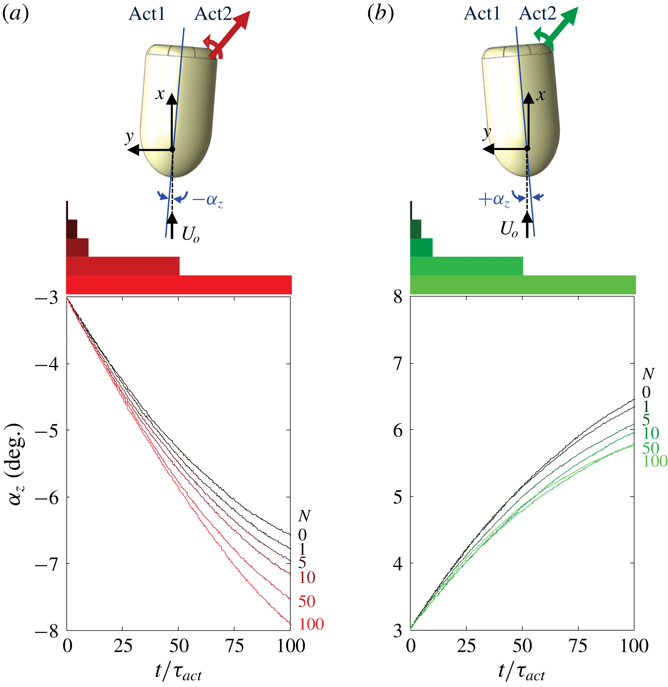
Figure 11. Time traces of the phase-averaged transient attitude of the model following the onset of open-loop pulse-modulated actuation of a single jet (Act2), leading to a CW moment as shown in insets with bursts of
 $N=0$
(base flow), 1, 5, 10, 50 and 100 actuation pulses. When the actuation is applied at
$N=0$
(base flow), 1, 5, 10, 50 and 100 actuation pulses. When the actuation is applied at
 $\unicode[STIX]{x1D6FC}_{z}=-3^{\circ }$
(a) it supports the motion and the model’s attitude increases, and when it is applied at
$\unicode[STIX]{x1D6FC}_{z}=-3^{\circ }$
(a) it supports the motion and the model’s attitude increases, and when it is applied at
 $\unicode[STIX]{x1D6FC}_{z}=+3^{\circ }$
(b) it resists the motion and the attitude decreases. The traces are shown in shades of red (
$\unicode[STIX]{x1D6FC}_{z}=+3^{\circ }$
(b) it resists the motion and the attitude decreases. The traces are shown in shades of red (
 $\unicode[STIX]{x1D6FC}_{z}=-3^{\circ }$
) and green (
$\unicode[STIX]{x1D6FC}_{z}=-3^{\circ }$
) and green (
 $\unicode[STIX]{x1D6FC}_{z}=+3^{\circ }$
) that vary from dark to light with increasing
$\unicode[STIX]{x1D6FC}_{z}=+3^{\circ }$
) that vary from dark to light with increasing
 $N$
(
$N$
(
 $N=0$
is marked in black). The bars above each graph show the corresponding durations of the actuation bursts.
$N=0$
is marked in black). The bars above each graph show the corresponding durations of the actuation bursts.
The cumulative effects of pulse-modulated actuation are demonstrated by tracking the changes in the model’s attitude
 $\unicode[STIX]{x1D6FC}_{z}$
(
$\unicode[STIX]{x1D6FC}_{z}$
(
 $t$
) following actuation by the same single jet at two opposite azimuthal angles
$t$
) following actuation by the same single jet at two opposite azimuthal angles
 $\unicode[STIX]{x1D6FC}_{z}=-3^{\circ }$
(figure 11
a) and
$\unicode[STIX]{x1D6FC}_{z}=-3^{\circ }$
(figure 11
a) and
 $+3^{\circ }$
(figure 11
b) when the model is rotating CW and CCW, respectively. These triggering points are chosen arbitrarily as half-amplitude estimates, to demonstrate the synthetic jet’s control authority when it tends to stabilize or destabilize the model, respectively. As shown by Lambert et al. (Reference Lambert, Vukasinovic and Glezer2015) and schematically in top views of the model in figure 11(a,b), when the actuator on the right rear surface of the model is used at these azimuthal attitudes, the
$+3^{\circ }$
(figure 11
b) when the model is rotating CW and CCW, respectively. These triggering points are chosen arbitrarily as half-amplitude estimates, to demonstrate the synthetic jet’s control authority when it tends to stabilize or destabilize the model, respectively. As shown by Lambert et al. (Reference Lambert, Vukasinovic and Glezer2015) and schematically in top views of the model in figure 11(a,b), when the actuator on the right rear surface of the model is used at these azimuthal attitudes, the
 $y$
-component of the induced aerodynamic side force acts to the right (in this view) and therefore the aerodynamic moment about the centre of rotation has the same CW sense as the angular motion
$y$
-component of the induced aerodynamic side force acts to the right (in this view) and therefore the aerodynamic moment about the centre of rotation has the same CW sense as the angular motion
 $\dot{\unicode[STIX]{x1D6FC}}_{z}$
in figure 11(a) (i.e. supporting the motion), and the opposite sense (i.e. opposing the motion) in figure 11(b). Therefore, the actuation tends to amplify (at
$\dot{\unicode[STIX]{x1D6FC}}_{z}$
in figure 11(a) (i.e. supporting the motion), and the opposite sense (i.e. opposing the motion) in figure 11(b). Therefore, the actuation tends to amplify (at
 $\unicode[STIX]{x1D6FC}_{z}=-3^{\circ }$
) or attenuate (at
$\unicode[STIX]{x1D6FC}_{z}=-3^{\circ }$
) or attenuate (at
 $\unicode[STIX]{x1D6FC}_{z}=+3^{\circ }$
) the amplitude of the lateral (base) oscillations in the absence of actuation. Pulse modulation is then effected with actuation bursts having
$\unicode[STIX]{x1D6FC}_{z}=+3^{\circ }$
) the amplitude of the lateral (base) oscillations in the absence of actuation. Pulse modulation is then effected with actuation bursts having
 $N=1$
, 5, 10, 50 and 100 successive actuation cycles of the synthetic jet. Following the termination of each burst, the model continues to oscillate freely for four lateral oscillation cycles before the actuation is reapplied on the next crossing through
$N=1$
, 5, 10, 50 and 100 successive actuation cycles of the synthetic jet. Following the termination of each burst, the model continues to oscillate freely for four lateral oscillation cycles before the actuation is reapplied on the next crossing through
 $\unicode[STIX]{x1D6FC}_{z}=-3^{\circ }$
or
$\unicode[STIX]{x1D6FC}_{z}=-3^{\circ }$
or
 $+3^{\circ }$
, and its effects are phase-averaged over such fifty realizations.
$+3^{\circ }$
, and its effects are phase-averaged over such fifty realizations.
The effects of burst actuation on the lateral motion of the model are demonstrated using time traces of the phase-averaged transitory attitude following the onset of the pulse-modulated actuation at
 $\unicode[STIX]{x1D6FC}_{z}=-3^{\circ }$
(figure 11
a) and
$\unicode[STIX]{x1D6FC}_{z}=-3^{\circ }$
(figure 11
a) and
 $+3^{\circ }$
(figure 11
b), where the bars at the top of each figure mark the duration of each of the five actuation bursts. When actuation is applied at
$+3^{\circ }$
(figure 11
b), where the bars at the top of each figure mark the duration of each of the five actuation bursts. When actuation is applied at
 $\unicode[STIX]{x1D6FC}_{z}=-3^{\circ }$
while the model moves CW, the induced aerodynamic moment enhances the lateral oscillation amplitude (as shown schematically in the inset), the actuation bursts result in a significant increase in the angular velocity of the model and consequently in
$\unicode[STIX]{x1D6FC}_{z}=-3^{\circ }$
while the model moves CW, the induced aerodynamic moment enhances the lateral oscillation amplitude (as shown schematically in the inset), the actuation bursts result in a significant increase in the angular velocity of the model and consequently in
 $\unicode[STIX]{x1D6FC}_{z}(t)$
compared to the base flow. In fact, it is remarkable that even a single actuation pulse (
$\unicode[STIX]{x1D6FC}_{z}(t)$
compared to the base flow. In fact, it is remarkable that even a single actuation pulse (
 $\unicode[STIX]{x1D70F}_{act}=0.0016\unicode[STIX]{x1D70F}_{z}$
) results in a measurable increase in the attitude, although its effect is not apparent (owing to the model’s inertia) until
$\unicode[STIX]{x1D70F}_{act}=0.0016\unicode[STIX]{x1D70F}_{z}$
) results in a measurable increase in the attitude, although its effect is not apparent (owing to the model’s inertia) until
 $t/\unicode[STIX]{x1D70F}_{act}>20$
, which is well after the actuation is terminated, and persists through
$t/\unicode[STIX]{x1D70F}_{act}>20$
, which is well after the actuation is terminated, and persists through
 $t/\unicode[STIX]{x1D70F}_{act}\approx 100$
. Larger increments of deflection are effected when the duration of the actuation burst (or the total resulting integral actuation effect) is increased. These effects of the actuation are clearly amplified by the attachment and vectoring of the separated shear layer to the Coanda surface at the aft of the model (cf. figure 10). Furthermore, the data in figure 10 also indicate that the relaxation time of the near wake following the termination of the actuation burst is significantly longer than the onset time, indicating that the temporal increase in the yawing moment persists well past the termination of the actuation. This is apparent from the monotonic increase in the time rate of change of
$t/\unicode[STIX]{x1D70F}_{act}\approx 100$
. Larger increments of deflection are effected when the duration of the actuation burst (or the total resulting integral actuation effect) is increased. These effects of the actuation are clearly amplified by the attachment and vectoring of the separated shear layer to the Coanda surface at the aft of the model (cf. figure 10). Furthermore, the data in figure 10 also indicate that the relaxation time of the near wake following the termination of the actuation burst is significantly longer than the onset time, indicating that the temporal increase in the yawing moment persists well past the termination of the actuation. This is apparent from the monotonic increase in the time rate of change of
 $\unicode[STIX]{x1D6FC}_{z}(t)$
following the termination of the actuation for
$\unicode[STIX]{x1D6FC}_{z}(t)$
following the termination of the actuation for
 $N=100$
compared to the base motion (it is also noteworthy that the initial delay in the effect of the actuation diminishes with increasing duration of the actuation burst). These effects of the actuation are reversed when it is applied at
$N=100$
compared to the base motion (it is also noteworthy that the initial delay in the effect of the actuation diminishes with increasing duration of the actuation burst). These effects of the actuation are reversed when it is applied at
 $\unicode[STIX]{x1D6FC}_{z}=+3^{\circ }$
as the model moves CCW (figure 11
b). Here, the primary effect of the actuation is a reduction in the attitude angle of the model compared to the base flow. Similar to the trends in figure 11(a), a single-jet pulse leads to a measurable reduction in attitude and in the angular yawing velocity, and although the delay to observable changes the model’s attitude is longer (
$\unicode[STIX]{x1D6FC}_{z}=+3^{\circ }$
as the model moves CCW (figure 11
b). Here, the primary effect of the actuation is a reduction in the attitude angle of the model compared to the base flow. Similar to the trends in figure 11(a), a single-jet pulse leads to a measurable reduction in attitude and in the angular yawing velocity, and although the delay to observable changes the model’s attitude is longer (
 $t/\unicode[STIX]{x1D70F}_{act}>55$
), the deceleration in the angular velocity persists past the end of the data record. Similar to the data in figure 11(a), the delay to reduction in the model’s attitude diminishes with increasing duration or of the actuation perturbation. However, while the reduction in the attitude angle intensifies monotonically with burst length up to
$t/\unicode[STIX]{x1D70F}_{act}>55$
), the deceleration in the angular velocity persists past the end of the data record. Similar to the data in figure 11(a), the delay to reduction in the model’s attitude diminishes with increasing duration or of the actuation perturbation. However, while the reduction in the attitude angle intensifies monotonically with burst length up to
 $N=10$
, the reduction for
$N=10$
, the reduction for
 $N=50$
is nearly identical to
$N=50$
is nearly identical to
 $N=100$
for
$N=100$
for
 $t/\unicode[STIX]{x1D70F}_{act}<45$
, is larger than
$t/\unicode[STIX]{x1D70F}_{act}<45$
, is larger than
 $N=100$
for
$N=100$
for
 $45<t/\unicode[STIX]{x1D70F}_{act}<60$
, and is lower than
$45<t/\unicode[STIX]{x1D70F}_{act}<60$
, and is lower than
 $N=100$
for
$N=100$
for
 $t/\unicode[STIX]{x1D70F}_{act}>90$
. It is conjectured that unlike actuation at
$t/\unicode[STIX]{x1D70F}_{act}>90$
. It is conjectured that unlike actuation at
 $\unicode[STIX]{x1D6FC}_{z}=-3^{\circ }$
, the less pronounced effect is associated with the changes in controlling the separating shear layer in the presence of an adverse pressure gradient in the upstream boundary layer.
$\unicode[STIX]{x1D6FC}_{z}=-3^{\circ }$
, the less pronounced effect is associated with the changes in controlling the separating shear layer in the presence of an adverse pressure gradient in the upstream boundary layer.

Figure 12. Phase plots of the model’s attitude in the presence of pulsed actuation
 $\unicode[STIX]{x1D6FC}_{z\text{-}act}$
relative to the corresponding attitude at the same period fraction in the base flow
$\unicode[STIX]{x1D6FC}_{z\text{-}act}$
relative to the corresponding attitude at the same period fraction in the base flow
 $\unicode[STIX]{x1D6FC}_{z\text{-}base}$
. The onset of the pulse-modulated actuation is at
$\unicode[STIX]{x1D6FC}_{z\text{-}base}$
. The onset of the pulse-modulated actuation is at
 $\unicode[STIX]{x1D6FC}_{zo}=-3^{\circ }$
(a,b) and
$\unicode[STIX]{x1D6FC}_{zo}=-3^{\circ }$
(a,b) and
 $+3^{\circ }$
(c,d) using the same colour maps as in figure 11: (a,c) magnified view of the model trajectories
$+3^{\circ }$
(c,d) using the same colour maps as in figure 11: (a,c) magnified view of the model trajectories
 $\unicode[STIX]{x1D6FC}_{zo}$
–
$\unicode[STIX]{x1D6FC}_{zo}$
–
 $\unicode[STIX]{x1D6FC}_{zmax}$
–
$\unicode[STIX]{x1D6FC}_{zmax}$
–
 $\unicode[STIX]{x1D6FC}_{zo}$
, and (b,d) during a full oscillation cycle.
$\unicode[STIX]{x1D6FC}_{zo}$
, and (b,d) during a full oscillation cycle.
The variation of the model’s phase-averaged attitude angle in the presence of pulsed actuation
 $\unicode[STIX]{x1D6FC}_{z\text{-}act}(t)$
(figure 11) is compared with the respective corresponding model attitude of the base flow
$\unicode[STIX]{x1D6FC}_{z\text{-}act}(t)$
(figure 11) is compared with the respective corresponding model attitude of the base flow
 $\unicode[STIX]{x1D6FC}_{z\text{-}base}(t)$
at the same times during the oscillation cycle. Actuations by Act2 effected at
$\unicode[STIX]{x1D6FC}_{z\text{-}base}(t)$
at the same times during the oscillation cycle. Actuations by Act2 effected at
 $\unicode[STIX]{x1D6FC}_{z}=-3^{\circ }$
(figure 11
a) and at
$\unicode[STIX]{x1D6FC}_{z}=-3^{\circ }$
(figure 11
a) and at
 $\unicode[STIX]{x1D6FC}_{z}=3^{\circ }$
(figure 11
b) are shown in figures 12(a,b) and 12(c,d), respectively. The yawing moment induced by the actuation in figure 12(a,b) leads to a monotonic increase in the magnitudes of the model’s lateral excursion, beginning with a single actuation pulse (approximately
$\unicode[STIX]{x1D6FC}_{z}=3^{\circ }$
(figure 11
b) are shown in figures 12(a,b) and 12(c,d), respectively. The yawing moment induced by the actuation in figure 12(a,b) leads to a monotonic increase in the magnitudes of the model’s lateral excursion, beginning with a single actuation pulse (approximately
 $0.3^{\circ }$
) and increasing with the number of jet pulses in the actuation burst
$0.3^{\circ }$
) and increasing with the number of jet pulses in the actuation burst
 $N$
up to nearly
$N$
up to nearly
 $1.9^{\circ }$
for
$1.9^{\circ }$
for
 $N=100$
. The data in figure 12(a) show that even though the longest actuation burst is terminated well before the model reaches its maximum lateral excursion, the model takes longer to return to the onset attitude as a result of the angular momentum imparted by the actuation. In fact, the maximum excursion angles following
$N=100$
. The data in figure 12(a) show that even though the longest actuation burst is terminated well before the model reaches its maximum lateral excursion, the model takes longer to return to the onset attitude as a result of the angular momentum imparted by the actuation. In fact, the maximum excursion angles following
 $N=1$
and 100 are
$N=1$
and 100 are
 $7.2^{\circ }$
and
$7.2^{\circ }$
and
 $8.9^{\circ }$
, respectively, and when the baseline model returns to
$8.9^{\circ }$
, respectively, and when the baseline model returns to
 $\unicode[STIX]{x1D6FC}_{z\text{-}base}=-3^{\circ }$
,
$\unicode[STIX]{x1D6FC}_{z\text{-}base}=-3^{\circ }$
,
 $\unicode[STIX]{x1D6FC}_{z\text{-}act}$
varies between
$\unicode[STIX]{x1D6FC}_{z\text{-}act}$
varies between
 $-3.4^{\circ }$
and
$-3.4^{\circ }$
and
 $-5.3^{\circ }$
when
$-5.3^{\circ }$
when
 $N$
varies between 1 and 100. It is noteworthy that, as the total pulsed perturbation is imparted by the actuation increases with
$N$
varies between 1 and 100. It is noteworthy that, as the total pulsed perturbation is imparted by the actuation increases with
 $N$
, the return trajectory of
$N$
, the return trajectory of
 $\unicode[STIX]{x1D6FC}_{z\text{-}act}$
when the change of slope of
$\unicode[STIX]{x1D6FC}_{z\text{-}act}$
when the change of slope of
 $\unicode[STIX]{x1D6FC}_{z\text{-}act}$
relative to
$\unicode[STIX]{x1D6FC}_{z\text{-}act}$
relative to
 $\unicode[STIX]{x1D6FC}_{z\text{-}base}$
varies only slightly and
$\unicode[STIX]{x1D6FC}_{z\text{-}base}$
varies only slightly and
 $\unicode[STIX]{x1D6FC}_{z\text{-}act}$
becomes offset relative to
$\unicode[STIX]{x1D6FC}_{z\text{-}act}$
becomes offset relative to
 $\unicode[STIX]{x1D6FC}_{z\text{-}base}$
. As a result of the actuation, the model’s maximum excursions increase during the second half of the cycle (figure 12
b), resulting in larger offset attitude when
$\unicode[STIX]{x1D6FC}_{z\text{-}base}$
. As a result of the actuation, the model’s maximum excursions increase during the second half of the cycle (figure 12
b), resulting in larger offset attitude when
 $\unicode[STIX]{x1D6FC}_{z\text{-}base}$
returns to zero. This response of the model indicates the receptivity of the flow to the actuation and the coupling between the model and its near wake. Similarly, when the actuation is applied with the intent of diminishing the model’s lateral oscillations (figure 12
c,d),
$\unicode[STIX]{x1D6FC}_{z\text{-}base}$
returns to zero. This response of the model indicates the receptivity of the flow to the actuation and the coupling between the model and its near wake. Similarly, when the actuation is applied with the intent of diminishing the model’s lateral oscillations (figure 12
c,d),
 $\unicode[STIX]{x1D6FC}_{z\text{-}act}$
decreases relative to
$\unicode[STIX]{x1D6FC}_{z\text{-}act}$
decreases relative to
 $\unicode[STIX]{x1D6FC}_{z\text{-}base}$
and the excursion amplitude is reduced, although the decrements are smaller than the increments in figure 12(a,b) (for
$\unicode[STIX]{x1D6FC}_{z\text{-}base}$
and the excursion amplitude is reduced, although the decrements are smaller than the increments in figure 12(a,b) (for
 $N=100$
, the reduction is approximately 1
$N=100$
, the reduction is approximately 1
 $^{\circ }$
in figure 12
d). As noted in connection with figure 11(b), the effect of the actuation with
$^{\circ }$
in figure 12
d). As noted in connection with figure 11(b), the effect of the actuation with
 $N=100$
seems to intensify following the termination of the actuation, and the data in figure 12(d) indicate a strong reduction in
$N=100$
seems to intensify following the termination of the actuation, and the data in figure 12(d) indicate a strong reduction in
 $\unicode[STIX]{x1D6FC}_{z\text{-}act}$
at the opposite end of the cycle (when
$\unicode[STIX]{x1D6FC}_{z\text{-}act}$
at the opposite end of the cycle (when
 $\unicode[STIX]{x1D6FC}_{z\text{-}base}$
is
$\unicode[STIX]{x1D6FC}_{z\text{-}base}$
is
 $-6.9^{\circ }$
and
$-6.9^{\circ }$
and
 $\unicode[STIX]{x1D6FC}_{z\text{-}act}$
is reduced to approximately
$\unicode[STIX]{x1D6FC}_{z\text{-}act}$
is reduced to approximately
 $-5.6^{\circ }$
).
$-5.6^{\circ }$
).
Transitory effects associated with the onset and termination of the actuation when it is applied on time scales that are long compared to the characteristic time scales of the response of the near wake are investigated using a single and the two opposite actuation jets. Figure 13 shows data extracted from the instantaneous time traces of the model’s attitude during 34 oscillation periods of the base flow (approximately
 $2400\unicode[STIX]{x1D70F}_{conv}$
) where actuation is activated and terminated at
$2400\unicode[STIX]{x1D70F}_{conv}$
) where actuation is activated and terminated at
 $t/\unicode[STIX]{x1D70F}_{conv}=600$
and 1800 relative to the beginning of the time trace record. The time traces of the model’s oscillations in the absence of actuation (base flow, shown in black in figure 13
a1,2) exhibit the characteristic cycle-to-cycle variations in amplitude and period of the model’s free oscillations (the nominal attitude is
$t/\unicode[STIX]{x1D70F}_{conv}=600$
and 1800 relative to the beginning of the time trace record. The time traces of the model’s oscillations in the absence of actuation (base flow, shown in black in figure 13
a1,2) exhibit the characteristic cycle-to-cycle variations in amplitude and period of the model’s free oscillations (the nominal attitude is
 $\bar{\unicode[STIX]{x1D6FC}}_{z}=0$
).
$\bar{\unicode[STIX]{x1D6FC}}_{z}=0$
).

Figure 13. Phase-averaged (25 realizations) traces of
 $\dot{\unicode[STIX]{x1D6FC}_{z}}$
and
$\dot{\unicode[STIX]{x1D6FC}_{z}}$
and
 $C_{Y}$
versus
$C_{Y}$
versus
 $a_{z}$
during (
$a_{z}$
during (
 $-100\unicode[STIX]{x1D70F}_{conv}<t<+600\unicode[STIX]{x1D70F}_{conv}$
) after the onset (at
$-100\unicode[STIX]{x1D70F}_{conv}<t<+600\unicode[STIX]{x1D70F}_{conv}$
) after the onset (at
 $\unicode[STIX]{x1D6FC}_{z}=3^{\circ }$
,
$\unicode[STIX]{x1D6FC}_{z}=3^{\circ }$
,
 $\dot{\unicode[STIX]{x1D6FC}_{z}}>0$
) and termination (
$\dot{\unicode[STIX]{x1D6FC}_{z}}>0$
) and termination (
 $1200\unicode[STIX]{x1D70F}_{conv}$
after onset) of single-jet actuation (10
a1,2 (
$1200\unicode[STIX]{x1D70F}_{conv}$
after onset) of single-jet actuation (10
a1,2 (
 $\dot{\unicode[STIX]{x1D6FC}_{z}}$
) and 10
a3,4 (
$\dot{\unicode[STIX]{x1D6FC}_{z}}$
) and 10
a3,4 (
 $C_{Y}$
)), and of two-jet actuation (10
b1,2 (
$C_{Y}$
)), and of two-jet actuation (10
b1,2 (
 $\dot{\unicode[STIX]{x1D6FC}_{z}}$
) and 10
b3,4 (
$\dot{\unicode[STIX]{x1D6FC}_{z}}$
) and 10
b3,4 (
 $C_{Y}$
)). The phase traces without actuation are marked in black and during actuation in blue (single jet) and green (two jets).
$C_{Y}$
)). The phase traces without actuation are marked in black and during actuation in blue (single jet) and green (two jets).
The evolution of the model’s trajectory during the time intervals about the onset and termination of single- (blue) and two-jet actuation (green) is displayed using phase plots of
 $\dot{\unicode[STIX]{x1D6FC}_{z}}$
versus
$\dot{\unicode[STIX]{x1D6FC}_{z}}$
versus
 $\unicode[STIX]{x1D6FC}_{z}$
(in figures 13
a1,2, b1,2) and of the computed aerodynamic yawing moment coefficient
$\unicode[STIX]{x1D6FC}_{z}$
(in figures 13
a1,2, b1,2) and of the computed aerodynamic yawing moment coefficient
 $C_{Y}$
(cf. § 3) versus
$C_{Y}$
(cf. § 3) versus
 $\unicode[STIX]{x1D6FC}_{z}$
(in figure 13
a3,4,b3,4). Each plot is generated by phase averaging 25 instantaneous realizations during a time interval ranging from
$\unicode[STIX]{x1D6FC}_{z}$
(in figure 13
a3,4,b3,4). Each plot is generated by phase averaging 25 instantaneous realizations during a time interval ranging from
 $100\unicode[STIX]{x1D70F}_{conv}$
(
$100\unicode[STIX]{x1D70F}_{conv}$
(
 $1.4\unicode[STIX]{x1D70F}_{z}$
) prior to through
$1.4\unicode[STIX]{x1D70F}_{z}$
) prior to through
 $600\unicode[STIX]{x1D70F}_{conv}$
(
$600\unicode[STIX]{x1D70F}_{conv}$
(
 $8.4\unicode[STIX]{x1D70F}_{z}$
) following the respective triggers of the onset and termination of the actuation. The traces of
$8.4\unicode[STIX]{x1D70F}_{z}$
) following the respective triggers of the onset and termination of the actuation. The traces of
 $\dot{\unicode[STIX]{x1D6FC}_{z}}$
and
$\dot{\unicode[STIX]{x1D6FC}_{z}}$
and
 $C_{Y}$
prior to and following the termination of the actuation are marked in black, and single- and two-jet actuations are marked in blue and green, respectively.
$C_{Y}$
prior to and following the termination of the actuation are marked in black, and single- and two-jet actuations are marked in blue and green, respectively.
The phase plots
 $\dot{\unicode[STIX]{x1D6FC}_{z}}$
–
$\dot{\unicode[STIX]{x1D6FC}_{z}}$
–
 $\unicode[STIX]{x1D6FC}_{z}$
in the base flow prior to the onset of the actuation (figures 13
a1,b1) exhibit a slightly tilted (elliptical) path which is a result of the lag (
$\unicode[STIX]{x1D6FC}_{z}$
in the base flow prior to the onset of the actuation (figures 13
a1,b1) exhibit a slightly tilted (elliptical) path which is a result of the lag (
 ${\sim}\unicode[STIX]{x03C0}/2$
) between the angular velocity and the nearly sinusoidal attitude. Following the onset of single-jet actuation, the mean attitude of the model is offset (to
${\sim}\unicode[STIX]{x03C0}/2$
) between the angular velocity and the nearly sinusoidal attitude. Following the onset of single-jet actuation, the mean attitude of the model is offset (to
 $\bar{\unicode[STIX]{x1D6FC}}_{z}\sim 3.2^{\circ }$
, figure 13
a1) within one oscillation cycle and the peak-to-peak variations in the attitude and angular velocity decrease from
$\bar{\unicode[STIX]{x1D6FC}}_{z}\sim 3.2^{\circ }$
, figure 13
a1) within one oscillation cycle and the peak-to-peak variations in the attitude and angular velocity decrease from
 $\pm 6.9^{\circ }$
to
$\pm 6.9^{\circ }$
to
 $\pm 5.5^{\circ }$
and from
$\pm 5.5^{\circ }$
and from
 $\pm 80\,^{\circ }\,\text{s}^{-1}$
to
$\pm 80\,^{\circ }\,\text{s}^{-1}$
to
 $\pm 60\,^{\circ }\,\text{s}^{-1}$
. Upon termination of actuation (figure 13
a2), the model exhibits a sharp change in
$\pm 60\,^{\circ }\,\text{s}^{-1}$
. Upon termination of actuation (figure 13
a2), the model exhibits a sharp change in
 $\unicode[STIX]{x1D6FC}_{z}$
(to the left) within a single oscillation cycle. The trajectory does not exhibit a full return to the base flow in figure 13(a1), indicating a relatively long relaxation time (over four lateral cycles) following the abrupt termination of the actuation.
$\unicode[STIX]{x1D6FC}_{z}$
(to the left) within a single oscillation cycle. The trajectory does not exhibit a full return to the base flow in figure 13(a1), indicating a relatively long relaxation time (over four lateral cycles) following the abrupt termination of the actuation.
The computed yawing moment
 $C_{Y}$
in the absence of actuation exhibits largely CW hysteresis loop caused by aerodynamic damping with a negative slant (to the left) as expected from the dominant yawing moment on a body in a nominally harmonic yaw motion. The moment phase trace includes small, nearly symmetric, CCW loops at its peak lateral excursions that are apparently associated with vorticity shedding as the direction of the lateral motion changes time-periodically (cf. § 3). When single-jet actuation is applied (figure 13
a3), the attitude offset of the primary CW loop is accompanied by a reduction in the range of
$C_{Y}$
in the absence of actuation exhibits largely CW hysteresis loop caused by aerodynamic damping with a negative slant (to the left) as expected from the dominant yawing moment on a body in a nominally harmonic yaw motion. The moment phase trace includes small, nearly symmetric, CCW loops at its peak lateral excursions that are apparently associated with vorticity shedding as the direction of the lateral motion changes time-periodically (cf. § 3). When single-jet actuation is applied (figure 13
a3), the attitude offset of the primary CW loop is accompanied by a reduction in the range of
 $C_{Y}$
(from
$C_{Y}$
(from
 $\pm 0.043$
to
$\pm 0.043$
to
 $\pm 0.034$
). Perhaps more prominent are the differences in the characteristics of
$\pm 0.034$
). Perhaps more prominent are the differences in the characteristics of
 $C_{Y}$
at the peak excursions. While the base flow loop about
$C_{Y}$
at the peak excursions. While the base flow loop about
 $\unicode[STIX]{x1D6FC}_{z}=-2.5^{\circ }$
nearly vanishes, the CCW loop at the peak deflection near
$\unicode[STIX]{x1D6FC}_{z}=-2.5^{\circ }$
nearly vanishes, the CCW loop at the peak deflection near
 $\unicode[STIX]{x1D6FC}_{z}=+8.5^{\circ }$
is significantly larger where
$\unicode[STIX]{x1D6FC}_{z}=+8.5^{\circ }$
is significantly larger where
 $C_{Y}$
appears to overshoot (approximately 0.01) and then is nearly invariant (approximately
$C_{Y}$
appears to overshoot (approximately 0.01) and then is nearly invariant (approximately
 $-0.024$
) within the range
$-0.024$
) within the range
 $+5^{\circ }<\unicode[STIX]{x1D6FC}_{z}<+9^{\circ }$
. These asymmetric changes in the restoring aerodynamic yawing moment are apparently associated with the choice of the (asymmetric) active actuation jet which effects a CW moment that supports/resists the motions towards the positive/negative peak excursions. This edge effect vanishes following the termination of the actuation (figure 13
a4). While the range of
$+5^{\circ }<\unicode[STIX]{x1D6FC}_{z}<+9^{\circ }$
. These asymmetric changes in the restoring aerodynamic yawing moment are apparently associated with the choice of the (asymmetric) active actuation jet which effects a CW moment that supports/resists the motions towards the positive/negative peak excursions. This edge effect vanishes following the termination of the actuation (figure 13
a4). While the range of
 $C_{Y}$
increases, it does not reach its full pre-actuation extent within eight cycles following the termination.
$C_{Y}$
increases, it does not reach its full pre-actuation extent within eight cycles following the termination.

Figure 14. Variation with
 $Re_{D}$
of the ratio between actuation-induced average deflection angle and the r.m.s. attitude in the absence of actuation,
$Re_{D}$
of the ratio between actuation-induced average deflection angle and the r.m.s. attitude in the absence of actuation,
 $\bar{\unicode[STIX]{x1D6FC}}_{z\text{-}act}/\tilde{\unicode[STIX]{x1D6FC}}_{z\text{-}base}$
using a single jet (a), and the ratio of the r.m.s. of the attitude using two-jet actuation to the r.m.s. attitude in the absence of actuation,
$\bar{\unicode[STIX]{x1D6FC}}_{z\text{-}act}/\tilde{\unicode[STIX]{x1D6FC}}_{z\text{-}base}$
using a single jet (a), and the ratio of the r.m.s. of the attitude using two-jet actuation to the r.m.s. attitude in the absence of actuation,
 $\tilde{\unicode[STIX]{x1D6FC}}_{z\text{-}act}/\tilde{\unicode[STIX]{x1D6FC}}_{z\text{-}base}$
(b).
$\tilde{\unicode[STIX]{x1D6FC}}_{z\text{-}act}/\tilde{\unicode[STIX]{x1D6FC}}_{z\text{-}base}$
(b).
The corresponding phase plots that are associated with the simultaneous actuation of two opposite jets activated at the same time are shown in figure 13(b1–4) (the phase traces in the presence of actuation are marked in green). In contrast to the rapid change in the model’s attitude by single-jet actuation, simultaneous actuation by the opposite jets leads to a slower transition to the new state. This is because the actuation jets effect opposite yawing moments (i.e. Act1 and Act2 exhibit a CCW and CW moment, respectively) that each vary somewhat with the model’s attitude during the oscillation cycle. Unlike the single-jet actuation, the model is effectively being acted on by the difference in the effects of these two jets, instead of the full effect of a jet, which results in a slow convergence (within approximately six oscillation cycles) to the new limit cycle of the model. This actuation has significantly smaller peak-to-peak attitude excursions (
 $\pm 3^{\circ }$
) and range of angular velocity (
$\pm 3^{\circ }$
) and range of angular velocity (
 $\pm 30\,^{\circ }\,\text{s}^{-1}$
) than the base flow. The limit cycle is finally reached when the spanwise yawing motion is diminished to the point where the cyclical variations in the actuation-induced yawing moments are virtually balanced (figure 13
b1). Upon termination of the actuation (figure 13
b2), the model returns to the base motion in a similar manner to the termination of the actuation in figure 13(a2) but, evidently, the lateral position and angular velocity of the model when the actuation is terminated lead to a different relaxation to the base limit cycle. The phase traces of
$\pm 30\,^{\circ }\,\text{s}^{-1}$
) than the base flow. The limit cycle is finally reached when the spanwise yawing motion is diminished to the point where the cyclical variations in the actuation-induced yawing moments are virtually balanced (figure 13
b1). Upon termination of the actuation (figure 13
b2), the model returns to the base motion in a similar manner to the termination of the actuation in figure 13(a2) but, evidently, the lateral position and angular velocity of the model when the actuation is terminated lead to a different relaxation to the base limit cycle. The phase traces of
 $C_{Y}$
indicate that the nominally symmetric actuation by the opposite jets (figure 13
b3) results in phase traces that have diminished ranges of
$C_{Y}$
indicate that the nominally symmetric actuation by the opposite jets (figure 13
b3) results in phase traces that have diminished ranges of
 $\unicode[STIX]{x1D6FC}_{z}$
and
$\unicode[STIX]{x1D6FC}_{z}$
and
 $C_{Y}$
(of approximately 60 % each) but are nominally similar to the traces of the base flow (including the details associated with shedding of vorticity concentrations at the edges of the lateral excursion). As with single-jet actuation, the return of the model to the base motion is incomplete at the end of the present data record within eight lateral time scales.
$C_{Y}$
(of approximately 60 % each) but are nominally similar to the traces of the base flow (including the details associated with shedding of vorticity concentrations at the edges of the lateral excursion). As with single-jet actuation, the return of the model to the base motion is incomplete at the end of the present data record within eight lateral time scales.
The effects of the flow speed on the effectiveness of the actuation are assessed using two characteristic measures, namely, the time-averaged change in the attitude of the model
 $\bar{\unicode[STIX]{x1D6FC}}_{z\text{-}act}$
during continuous single-jet actuation (cf. figure 13
a1), and the r.m.s. variation of the attitude
$\bar{\unicode[STIX]{x1D6FC}}_{z\text{-}act}$
during continuous single-jet actuation (cf. figure 13
a1), and the r.m.s. variation of the attitude
 $\tilde{\unicode[STIX]{x1D6FC}}_{z\text{-}act}$
when both jets are continuously active (cf. figure 13
b1). Each of these measures is normalized by the r.m.s. of the model’s attitude in the absence of actuation
$\tilde{\unicode[STIX]{x1D6FC}}_{z\text{-}act}$
when both jets are continuously active (cf. figure 13
b1). Each of these measures is normalized by the r.m.s. of the model’s attitude in the absence of actuation
 $\tilde{\unicode[STIX]{x1D6FC}}_{z\text{-}base}$
, which increases approximately linearly with
$\tilde{\unicode[STIX]{x1D6FC}}_{z\text{-}base}$
, which increases approximately linearly with
 $Re_{D}$
(cf. figure 4
a), and their variation with
$Re_{D}$
(cf. figure 4
a), and their variation with
 $Re_{D}$
within the range
$Re_{D}$
within the range
 $0.6\times 10^{5}<Re_{D}<2\times 10^{5}$
is shown in figures 14(a) and 14(b), respectively. The data in figure 14(a) show that
$0.6\times 10^{5}<Re_{D}<2\times 10^{5}$
is shown in figures 14(a) and 14(b), respectively. The data in figure 14(a) show that
 $\bar{\unicode[STIX]{x1D6FC}}_{z\text{-}act}$
increases monotonically with
$\bar{\unicode[STIX]{x1D6FC}}_{z\text{-}act}$
increases monotonically with
 $Re_{D}$
and reaches approximately
$Re_{D}$
and reaches approximately
 $0.7\tilde{\unicode[STIX]{x1D6FC}}_{z\text{-}base}$
(or approximately half of the base amplitude) at
$0.7\tilde{\unicode[STIX]{x1D6FC}}_{z\text{-}base}$
(or approximately half of the base amplitude) at
 $Re_{D}\geqslant 1.15\times 10^{5}$
, and remains nearly invariant thereafter, indicating that the induced attitude deflection increases approximately linearly with flow speed within the range tested. A similar pattern is shown when actuation is applied using two opposing jets in figure 14(b). The magnitude of
$Re_{D}\geqslant 1.15\times 10^{5}$
, and remains nearly invariant thereafter, indicating that the induced attitude deflection increases approximately linearly with flow speed within the range tested. A similar pattern is shown when actuation is applied using two opposing jets in figure 14(b). The magnitude of
 $\tilde{\unicode[STIX]{x1D6FC}}_{z\text{-}act}$
diminishes monotonically down to 0.35
$\tilde{\unicode[STIX]{x1D6FC}}_{z\text{-}act}$
diminishes monotonically down to 0.35
 $\tilde{\unicode[STIX]{x1D6FC}}_{z\text{-}base}$
and then appears to saturate for
$\tilde{\unicode[STIX]{x1D6FC}}_{z\text{-}base}$
and then appears to saturate for
 $Re_{D}>1.15\times 10^{5}$
, indicating a linear increase with flow speed (or reduction in suppression) at least through
$Re_{D}>1.15\times 10^{5}$
, indicating a linear increase with flow speed (or reduction in suppression) at least through
 $Re_{D}\approx 1.72\times 10^{5}$
that is followed by a somewhat steeper decrease in suppression for
$Re_{D}\approx 1.72\times 10^{5}$
that is followed by a somewhat steeper decrease in suppression for
 $Re_{D}>2.0\times 10^{5}$
. The momentum of the actuation (synthetic) jet was limited by the performance of its piezoelectric driver, and therefore was kept constant during the experiments in order to avoid damage to the driver at higher jet speeds. Consequently, its momentum coefficient (defined in § 2) decreased with increasing
$Re_{D}>2.0\times 10^{5}$
. The momentum of the actuation (synthetic) jet was limited by the performance of its piezoelectric driver, and therefore was kept constant during the experiments in order to avoid damage to the driver at higher jet speeds. Consequently, its momentum coefficient (defined in § 2) decreased with increasing
 $Re_{D}$
. However, the fact that the deflection of offset attitude saturates during the operation of a single jet even though its momentum coefficient decreases (figure 14
b) indicates that the effectiveness of the actuation actually increases with
$Re_{D}$
. However, the fact that the deflection of offset attitude saturates during the operation of a single jet even though its momentum coefficient decreases (figure 14
b) indicates that the effectiveness of the actuation actually increases with
 $Re_{D}$
.
$Re_{D}$
.

Figure 15. Time traces of the model’s instantaneous attitude,
 $\unicode[STIX]{x1D6FC}_{z}$
, during PID closed-loop attitude control: stabilizing the model about
$\unicode[STIX]{x1D6FC}_{z}$
, during PID closed-loop attitude control: stabilizing the model about
 $\unicode[STIX]{x1D6FC}_{z}=0^{\circ }$
(a) and
$\unicode[STIX]{x1D6FC}_{z}=0^{\circ }$
(a) and
 $2^{\circ }$
(b), and deliberate amplification of the base flow oscillations (c). Following activation (at
$2^{\circ }$
(b), and deliberate amplification of the base flow oscillations (c). Following activation (at
 $\unicode[STIX]{x1D6FC}_{z}=3^{\circ }$
,
$\unicode[STIX]{x1D6FC}_{z}=3^{\circ }$
,
 $\text{d}\unicode[STIX]{x1D6FC}_{z}/\text{d}t>0$
), control is applied for
$\text{d}\unicode[STIX]{x1D6FC}_{z}/\text{d}t>0$
), control is applied for
 $17\unicode[STIX]{x1D70F}_{z}$
(
$17\unicode[STIX]{x1D70F}_{z}$
(
 $1200\unicode[STIX]{x1D70F}_{conv}$
). The onset and termination of the actuation are marked by dashed lines (
$1200\unicode[STIX]{x1D70F}_{conv}$
). The onset and termination of the actuation are marked by dashed lines (
 $Re_{D}=1.15\times 10^{5}$
).
$Re_{D}=1.15\times 10^{5}$
).
5 Closed-loop flow actuation
Building on the results discussed in § 4, a PID feedback controller (Lambert Reference Lambert2016) is used to effect pulsed-modulated jet actuation with the objective of achieving a desired attitude of the free-yawing body. The controller (cf. the Appendix) generates actuation bursts each comprising a variable number of jet pulses that are similar, in principle, to the open-loop actuation investigated in connection with figures 11 and 12. Three programs for attitude control are investigated, namely, stabilizing the model about
 $\unicode[STIX]{x1D6FC}_{z}=0^{\circ }$
, steering the model to a prescribed attitude offset
$\unicode[STIX]{x1D6FC}_{z}=0^{\circ }$
, steering the model to a prescribed attitude offset
 $\unicode[STIX]{x1D6FC}_{z}>0^{\circ }$
, and deliberate amplification of the base flow oscillations (these programs are initially demonstrated at
$\unicode[STIX]{x1D6FC}_{z}>0^{\circ }$
, and deliberate amplification of the base flow oscillations (these programs are initially demonstrated at
 $Re_{D}=1.15\times 10^{5}$
). Time traces of the model’s attitude
$Re_{D}=1.15\times 10^{5}$
). Time traces of the model’s attitude
 $\unicode[STIX]{x1D6FC}_{z}(t)$
in figure 15(a–c) demonstrate the respective evolution of closed-loop control following the onset of each of the actuation programs. Similar to the traces that show the response of the model’s attitude to open-loop actuation, the PID control is applied for
$\unicode[STIX]{x1D6FC}_{z}(t)$
in figure 15(a–c) demonstrate the respective evolution of closed-loop control following the onset of each of the actuation programs. Similar to the traces that show the response of the model’s attitude to open-loop actuation, the PID control is applied for
 $1200\unicode[STIX]{x1D70F}_{conv}(17\unicode[STIX]{x1D70F}_{z})$
and triggered at
$1200\unicode[STIX]{x1D70F}_{conv}(17\unicode[STIX]{x1D70F}_{z})$
and triggered at
 $\unicode[STIX]{x1D6FC}_{z}=3^{\circ }$
when
$\unicode[STIX]{x1D6FC}_{z}=3^{\circ }$
when
 $\dot{\unicode[STIX]{x1D6FC}}_{z}>0$
(the onset and termination of the actuation are marked). Figure 15(a) shows that the controller stabilizes the model about
$\dot{\unicode[STIX]{x1D6FC}}_{z}>0$
(the onset and termination of the actuation are marked). Figure 15(a) shows that the controller stabilizes the model about
 $\unicode[STIX]{x1D6FC}_{z}=0^{\circ }$
within approximately
$\unicode[STIX]{x1D6FC}_{z}=0^{\circ }$
within approximately
 $2\unicode[STIX]{x1D70F}_{z}$
and the oscillation amplitude is significantly reduced such that
$2\unicode[STIX]{x1D70F}_{z}$
and the oscillation amplitude is significantly reduced such that
 $\unicode[STIX]{x1D6FC}_{z,rms}$
decreases by 90 % from nominally
$\unicode[STIX]{x1D6FC}_{z,rms}$
decreases by 90 % from nominally
 $4.9^{\circ }$
to
$4.9^{\circ }$
to
 $0.5^{\circ }$
and its frequency increases to 5.5 Hz (compared to 1.7 Hz of the base model). As discussed in connection with open-loop control (cf. figure 13), when the control is terminated, the relaxation of the model’s motion to the limit cycle of the base flow is significantly longer (approximately
$0.5^{\circ }$
and its frequency increases to 5.5 Hz (compared to 1.7 Hz of the base model). As discussed in connection with open-loop control (cf. figure 13), when the control is terminated, the relaxation of the model’s motion to the limit cycle of the base flow is significantly longer (approximately
 $8\unicode[STIX]{x1D70F}_{z}$
), which is commensurate with the inherently longer relaxation time of the separating shear layer on the aft segment of the model and the near wake. The time trace of the model’s attitude when the control goal is to steer the model to a steady attitude
$8\unicode[STIX]{x1D70F}_{z}$
), which is commensurate with the inherently longer relaxation time of the separating shear layer on the aft segment of the model and the near wake. The time trace of the model’s attitude when the control goal is to steer the model to a steady attitude
 $\unicode[STIX]{x1D6FC}_{z}=2^{\circ }$
is shown in figure 15(b). These data show that the characteristic time needed for stabilizing about the off-axis attitude is longer than about
$\unicode[STIX]{x1D6FC}_{z}=2^{\circ }$
is shown in figure 15(b). These data show that the characteristic time needed for stabilizing about the off-axis attitude is longer than about
 $\unicode[STIX]{x1D6FC}_{z}=0^{\circ }$
, or approximately
$\unicode[STIX]{x1D6FC}_{z}=0^{\circ }$
, or approximately
 $3\unicode[STIX]{x1D70F}_{z}$
and is clearly connected with overcoming the restoring side force of the base flow (
$3\unicode[STIX]{x1D70F}_{z}$
and is clearly connected with overcoming the restoring side force of the base flow (
 $\unicode[STIX]{x1D6FC}_{z,rms}$
of the oscillation is decreased by approximately 85 % to
$\unicode[STIX]{x1D6FC}_{z,rms}$
of the oscillation is decreased by approximately 85 % to
 $0.7^{\circ }$
). Amplification of the model’s oscillations about
$0.7^{\circ }$
). Amplification of the model’s oscillations about
 $\unicode[STIX]{x1D6FC}_{z}=0^{\circ }$
(figure 15
c) yields a significant increase in
$\unicode[STIX]{x1D6FC}_{z}=0^{\circ }$
(figure 15
c) yields a significant increase in
 $\unicode[STIX]{x1D6FC}_{z,rms}$
to
$\unicode[STIX]{x1D6FC}_{z,rms}$
to
 $8.6^{\circ }$
(approximately 175 %), where the characteristic times of the onset and termination (approximately
$8.6^{\circ }$
(approximately 175 %), where the characteristic times of the onset and termination (approximately
 $2\unicode[STIX]{x1D70F}_{z}$
and
$2\unicode[STIX]{x1D70F}_{z}$
and
 $8\unicode[STIX]{x1D70F}_{z}$
) are similar to the corresponding times for the model stabilization (figure 15
a).
$8\unicode[STIX]{x1D70F}_{z}$
) are similar to the corresponding times for the model stabilization (figure 15
a).
It is instructive to consider how the controller implements the actuation. Figure 16(a1–c1) show instantaneous time traces of
 $\unicode[STIX]{x1D6FC}_{z}(t)$
corresponding to figure 15(a–c), respectively, prior to and following the onset of feedback control. For simplicity, the onset of the actuation (
$\unicode[STIX]{x1D6FC}_{z}(t)$
corresponding to figure 15(a–c), respectively, prior to and following the onset of feedback control. For simplicity, the onset of the actuation (
 $\unicode[STIX]{x1D6FC}_{z}=3^{\circ }$
,
$\unicode[STIX]{x1D6FC}_{z}=3^{\circ }$
,
 $\dot{\unicode[STIX]{x1D6FC}}_{z}>0$
) is marked by
$\dot{\unicode[STIX]{x1D6FC}}_{z}>0$
) is marked by
 $t=0$
, such that
$t=0$
, such that
 $-100<t/\unicode[STIX]{x1D70F}_{conv}<+300$
, and the respective responses of the model’s attitude to stabilization around
$-100<t/\unicode[STIX]{x1D70F}_{conv}<+300$
, and the respective responses of the model’s attitude to stabilization around
 $\unicode[STIX]{x1D6FC}_{z}=0^{\circ }$
and
$\unicode[STIX]{x1D6FC}_{z}=0^{\circ }$
and
 $2^{\circ }$
are shown in figure 16(a1,b1), and to amplified oscillations in figure 16(c1). Also shown in figure 16(a2–c2) and in figure 16(a3–c3) are time traces of the corresponding amplitude modulation of the Act1 [Mod1(
$2^{\circ }$
are shown in figure 16(a1,b1), and to amplified oscillations in figure 16(c1). Also shown in figure 16(a2–c2) and in figure 16(a3–c3) are time traces of the corresponding amplitude modulation of the Act1 [Mod1(
 $t$
)] and Act2
$t$
)] and Act2
 $[\text{Mod}_{2}(t)]$
actuators (cf. figure 1). When the model is stabilized about
$[\text{Mod}_{2}(t)]$
actuators (cf. figure 1). When the model is stabilized about
 $\unicode[STIX]{x1D6FC}_{z}=0^{\circ }$
, the controller uses Act1 and Act2 in alternation to diminish
$\unicode[STIX]{x1D6FC}_{z}=0^{\circ }$
, the controller uses Act1 and Act2 in alternation to diminish
 $\dot{\unicode[STIX]{x1D6FC}}$
and reduce the excursions in the model’s attitude (as discussed in connection with figure 11). The actuation sequence begins with activation of Act2 (at 100 % modulation,
$\dot{\unicode[STIX]{x1D6FC}}$
and reduce the excursions in the model’s attitude (as discussed in connection with figure 11). The actuation sequence begins with activation of Act2 (at 100 % modulation,
 $0<t/\unicode[STIX]{x1D70F}_{conv}<9$
, figure 16
a3) when
$0<t/\unicode[STIX]{x1D70F}_{conv}<9$
, figure 16
a3) when
 $\dot{\unicode[STIX]{x1D6FC}}_{z}>0$
and it is terminated when
$\dot{\unicode[STIX]{x1D6FC}}_{z}>0$
and it is terminated when
 $\unicode[STIX]{x1D6FC}_{z}(t)$
has a local peak (
$\unicode[STIX]{x1D6FC}_{z}(t)$
has a local peak (
 $5.9^{\circ }$
,
$5.9^{\circ }$
,
 $t=13\unicode[STIX]{x1D70F}_{conv}$
) so the induced CW moment opposes the motion. This is followed by activation of Act1 (at 100 % modulation,
$t=13\unicode[STIX]{x1D70F}_{conv}$
) so the induced CW moment opposes the motion. This is followed by activation of Act1 (at 100 % modulation,
 $17<t/\unicode[STIX]{x1D70F}_{conv}<41$
, figure 16
a2) when
$17<t/\unicode[STIX]{x1D70F}_{conv}<41$
, figure 16
a2) when
 $\dot{\unicode[STIX]{x1D6FC}}_{z}<0$
until the model reaches its next maximum excursion (
$\dot{\unicode[STIX]{x1D6FC}}_{z}<0$
until the model reaches its next maximum excursion (
 $-4.0^{\circ }$
,
$-4.0^{\circ }$
,
 $t=44\unicode[STIX]{x1D70F}_{conv}$
) so that the induced CCW moment again opposes the motion. Subsequently, when
$t=44\unicode[STIX]{x1D70F}_{conv}$
) so that the induced CCW moment again opposes the motion. Subsequently, when
 $\dot{\unicode[STIX]{x1D6FC}}_{z}$
changes direction and Act2 is activated again (100 % modulation,
$\dot{\unicode[STIX]{x1D6FC}}_{z}$
changes direction and Act2 is activated again (100 % modulation,
 $47<t/\unicode[STIX]{x1D70F}_{conv}<70$
, figure 16
a3) and the induced CW moment continues to oppose the angular motion. Upon the termination of the third modulation pulse, the model’s maximum excursion diminishes to
$47<t/\unicode[STIX]{x1D70F}_{conv}<70$
, figure 16
a3) and the induced CW moment continues to oppose the angular motion. Upon the termination of the third modulation pulse, the model’s maximum excursion diminishes to
 $+3.1^{\circ }$
(
$+3.1^{\circ }$
(
 $t=74\unicode[STIX]{x1D70F}_{conv}$
), and as the next (fourth) modulation of Act1 (
$t=74\unicode[STIX]{x1D70F}_{conv}$
), and as the next (fourth) modulation of Act1 (
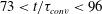 $73<t/\unicode[STIX]{x1D70F}_{conv}<96$
) diminishes the peak excursion to
$73<t/\unicode[STIX]{x1D70F}_{conv}<96$
) diminishes the peak excursion to
 $-1.7^{\circ }$
(
$-1.7^{\circ }$
(
 $t=100\unicode[STIX]{x1D70F}_{conv}$
), the controller decreases the magnitude of modulation as the model reaches its next peak excursion. Following this initial sequence, the controller activates Act1 and Act2 in alternation for disturbance rejection using brief modulation pulses (approximately
$t=100\unicode[STIX]{x1D70F}_{conv}$
), the controller decreases the magnitude of modulation as the model reaches its next peak excursion. Following this initial sequence, the controller activates Act1 and Act2 in alternation for disturbance rejection using brief modulation pulses (approximately
 $11\unicode[STIX]{x1D70F}_{conv}$
per actuator) at modulation levels that are below 50 % (figure 16
a2,3).
$11\unicode[STIX]{x1D70F}_{conv}$
per actuator) at modulation levels that are below 50 % (figure 16
a2,3).

Figure 16. Time traces of the model attitude,
 $\unicode[STIX]{x1D6FC}_{z}$
, prior to and immediately following the onset of closed-loop control
$\unicode[STIX]{x1D6FC}_{z}$
, prior to and immediately following the onset of closed-loop control
 $-100\unicode[STIX]{x1D70F}_{conv}<t<+300\unicode[STIX]{x1D70F}_{conv}$
(control is applied at
$-100\unicode[STIX]{x1D70F}_{conv}<t<+300\unicode[STIX]{x1D70F}_{conv}$
(control is applied at
 $\unicode[STIX]{x1D6FC}_{z}=3^{\circ }$
,
$\unicode[STIX]{x1D6FC}_{z}=3^{\circ }$
,
 $\dot{\unicode[STIX]{x1D6FC}_{z}}>0$
): stabilizing around
$\dot{\unicode[STIX]{x1D6FC}_{z}}>0$
): stabilizing around
 $\unicode[STIX]{x1D6FC}_{z}=0^{\circ }$
(a1, cf. figure 17
a) and
$\unicode[STIX]{x1D6FC}_{z}=0^{\circ }$
(a1, cf. figure 17
a) and
 $2^{\circ }$
(b1, cf. figure 17
b), and amplifying oscillations (c1, cf. figure 17
c). Also shown are the corresponding amplitude modulation waveforms of Act1: Mod1(
$2^{\circ }$
(b1, cf. figure 17
b), and amplifying oscillations (c1, cf. figure 17
c). Also shown are the corresponding amplitude modulation waveforms of Act1: Mod1(
 $t$
) in (a2–c2), and Act2: Mod2(
$t$
) in (a2–c2), and Act2: Mod2(
 $t$
) in (a3–c3) (
$t$
) in (a3–c3) (
 $C_{\unicode[STIX]{x1D707},max}=0.003$
).
$C_{\unicode[STIX]{x1D707},max}=0.003$
).

Figure 17. Phase-averaged plots of the model’s angular velocity
 $\dot{\unicode[STIX]{x1D6FC}_{z}}(t)$
, and of the (computed) yawing moment,
$\dot{\unicode[STIX]{x1D6FC}_{z}}(t)$
, and of the (computed) yawing moment,
 $C_{Y}$
, with respect to the model’s attitude,
$C_{Y}$
, with respect to the model’s attitude,
 $\unicode[STIX]{x1D6FC}_{z}$
. (a–c) correspond to the closed-loop actuation programs in figure 18(a–c) (i.e. attitude stabilization about
$\unicode[STIX]{x1D6FC}_{z}$
. (a–c) correspond to the closed-loop actuation programs in figure 18(a–c) (i.e. attitude stabilization about
 $\unicode[STIX]{x1D6FC}_{z}=0^{\circ }$
and
$\unicode[STIX]{x1D6FC}_{z}=0^{\circ }$
and
 $2^{\circ }$
, and oscillation amplification, respectively). These data are captured after (
$2^{\circ }$
, and oscillation amplification, respectively). These data are captured after (
 $-100\unicode[STIX]{x1D70F}_{conv}<t<+600\unicode[STIX]{x1D70F}_{conv}$
) the onset (rows 1 and 3) and termination (rows 2 and 4) of the actuation in each program. The segments of phase traces in the presence of each of the control programs control in (a–c) are marked in green, blue and red, respectively.
$-100\unicode[STIX]{x1D70F}_{conv}<t<+600\unicode[STIX]{x1D70F}_{conv}$
) the onset (rows 1 and 3) and termination (rows 2 and 4) of the actuation in each program. The segments of phase traces in the presence of each of the control programs control in (a–c) are marked in green, blue and red, respectively.

Figure 18. Variation with
 $Re_{D}$
of the ratio between actuation-induced stabilized deflection angle and the r.m.s. attitude in the absence of actuation
$Re_{D}$
of the ratio between actuation-induced stabilized deflection angle and the r.m.s. attitude in the absence of actuation
 $\bar{\unicode[STIX]{x1D6FC}}_{z-act}/\tilde{\unicode[STIX]{x1D6FC}}_{z-base}$
using closed-loop control (a), and the ratio of the r.m.s. of the attitude of closed-loop oscillation suppression (green) and oscillation amplification (red) to the r.m.s. attitude in the absence of actuation
$\bar{\unicode[STIX]{x1D6FC}}_{z-act}/\tilde{\unicode[STIX]{x1D6FC}}_{z-base}$
using closed-loop control (a), and the ratio of the r.m.s. of the attitude of closed-loop oscillation suppression (green) and oscillation amplification (red) to the r.m.s. attitude in the absence of actuation
 $\tilde{\unicode[STIX]{x1D6FC}}_{z-act}/\tilde{\unicode[STIX]{x1D6FC}}_{z-base}$
(b).
$\tilde{\unicode[STIX]{x1D6FC}}_{z-act}/\tilde{\unicode[STIX]{x1D6FC}}_{z-base}$
(b).
By comparison, for offset attitude of
 $\unicode[STIX]{x1D6FC}_{z}=2^{\circ }$
(figure 16
b1–3) the controller utilizes only Act1 (figure 16
b2) for inducing an asymmetric side force (and CW moment) to balance the restoring yawing moment of the base flow. The side force is applied as the model rotates between its positive and negative attitude excursions (i.e.
$\unicode[STIX]{x1D6FC}_{z}=2^{\circ }$
(figure 16
b1–3) the controller utilizes only Act1 (figure 16
b2) for inducing an asymmetric side force (and CW moment) to balance the restoring yawing moment of the base flow. The side force is applied as the model rotates between its positive and negative attitude excursions (i.e.
 $\dot{\unicode[STIX]{x1D6FC}}_{z}<0$
) where 100 % modulation is applied during
$\dot{\unicode[STIX]{x1D6FC}}_{z}<0$
) where 100 % modulation is applied during
 $11<t/\unicode[STIX]{x1D70F}_{conv}<39(6.9^{\circ }>\unicode[STIX]{x1D6FC}_{z}(t)>-3.3^{\circ })$
,
$11<t/\unicode[STIX]{x1D70F}_{conv}<39(6.9^{\circ }>\unicode[STIX]{x1D6FC}_{z}(t)>-3.3^{\circ })$
,
 $67<t/\unicode[STIX]{x1D70F}_{conv}<98(5.9^{\circ }>\unicode[STIX]{x1D6FC}_{z}(t)>-2.4^{\circ })$
, and
$67<t/\unicode[STIX]{x1D70F}_{conv}<98(5.9^{\circ }>\unicode[STIX]{x1D6FC}_{z}(t)>-2.4^{\circ })$
, and
 $126<t/\unicode[STIX]{x1D70F}_{conv}<157(4.5^{\circ }>\unicode[STIX]{x1D6FC}_{z}(t)>-0.8^{\circ })$
, while the peak excursions diminish monotonically. This explains why it takes the model longer to reach the stabilized attitude in figure 15(b) compared to figure 15(a) (approximately
$126<t/\unicode[STIX]{x1D70F}_{conv}<157(4.5^{\circ }>\unicode[STIX]{x1D6FC}_{z}(t)>-0.8^{\circ })$
, while the peak excursions diminish monotonically. This explains why it takes the model longer to reach the stabilized attitude in figure 15(b) compared to figure 15(a) (approximately
 $165\unicode[STIX]{x1D70F}_{conv}$
versus
$165\unicode[STIX]{x1D70F}_{conv}$
versus
 $110\unicode[STIX]{x1D70F}_{conv}$
). Also, the magnitude of the modulation pulses that are needed for disturbance rejection following the initial stabilization is higher (up to 75 %). This maximum steady offset control could also be achieved by using both jets (cf. the Appendix,
$110\unicode[STIX]{x1D70F}_{conv}$
). Also, the magnitude of the modulation pulses that are needed for disturbance rejection following the initial stabilization is higher (up to 75 %). This maximum steady offset control could also be achieved by using both jets (cf. the Appendix,
 $C_{1}=C_{2}=1$
). However, if the opposing jet had been activated, the model would have stabilized faster at a smaller
$C_{1}=C_{2}=1$
). However, if the opposing jet had been activated, the model would have stabilized faster at a smaller
 $\unicode[STIX]{x1D6FC}_{z}$
and then drift to its maximum offset angle in the
$\unicode[STIX]{x1D6FC}_{z}$
and then drift to its maximum offset angle in the
 $+\unicode[STIX]{x1D6FC}_{z}$
direction, as the Act2 diminishes to 0 % modulation. Using both jets for this control goal would lead to a model that stabilizes quicker than with one jet, but reaches the state of being both stabilized and centred around the desired offset angle slower.
$+\unicode[STIX]{x1D6FC}_{z}$
direction, as the Act2 diminishes to 0 % modulation. Using both jets for this control goal would lead to a model that stabilizes quicker than with one jet, but reaches the state of being both stabilized and centred around the desired offset angle slower.
For amplification of the yaw oscillation (figure 16
c1), Act1 is first activated when the model moves with
 $\dot{\unicode[STIX]{x1D6FC}}_{z}>0$
,
$\dot{\unicode[STIX]{x1D6FC}}_{z}>0$
,
 $0<t/\unicode[STIX]{x1D70F}_{conv}<15$
(figure 16
c2) and the induced CW moment supports the motion and increases the excursion amplitude. Thereafter, the modulation commands Mod1(
$0<t/\unicode[STIX]{x1D70F}_{conv}<15$
(figure 16
c2) and the induced CW moment supports the motion and increases the excursion amplitude. Thereafter, the modulation commands Mod1(
 $t$
) and Mod2(
$t$
) and Mod2(
 $t$
) (figure 16
c2,3) are nearly out of phase, and the sense of the induced aerodynamic moments is the same as the model’s angular velocity, while the degree of modulation is kept at nearly 100 %. It should be noted that, since the control authority of Act2 is somewhat lower than Act1, the controller compensates by using longer modulation periods, as depicted by Mod2(
$t$
) (figure 16
c2,3) are nearly out of phase, and the sense of the induced aerodynamic moments is the same as the model’s angular velocity, while the degree of modulation is kept at nearly 100 %. It should be noted that, since the control authority of Act2 is somewhat lower than Act1, the controller compensates by using longer modulation periods, as depicted by Mod2(
 $t$
) (this is also evident in the larger fluctuations of Mod2(
$t$
) (this is also evident in the larger fluctuations of Mod2(
 $t$
) in figure 16
a3 for
$t$
) in figure 16
a3 for
 $t>100\unicode[STIX]{x1D70F}_{conv}$
).
$t>100\unicode[STIX]{x1D70F}_{conv}$
).
Phase-averaged traces of the variation of the model’s angular velocity
 $\dot{\unicode[STIX]{x1D6FC}_{z}}$
, and the (computed) yawing moment
$\dot{\unicode[STIX]{x1D6FC}_{z}}$
, and the (computed) yawing moment
 $C_{Y}$
(cf. § 3) with its attitude
$C_{Y}$
(cf. § 3) with its attitude
 $\unicode[STIX]{x1D6FC}_{z}$
during the closed-loop actuation programs of figures 15(a–c) are shown, respectively, in figure 17(a–c). Phase-averaged traces (each over 25 realizations) are plotted during the interval
$\unicode[STIX]{x1D6FC}_{z}$
during the closed-loop actuation programs of figures 15(a–c) are shown, respectively, in figure 17(a–c). Phase-averaged traces (each over 25 realizations) are plotted during the interval
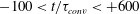 $-100<t/\unicode[STIX]{x1D70F}_{conv}<+600$
relative to the onset (a1,3, b1,3 and c1,3) and termination (a2,4, b2,4 and c2,4) of the actuation for
$-100<t/\unicode[STIX]{x1D70F}_{conv}<+600$
relative to the onset (a1,3, b1,3 and c1,3) and termination (a2,4, b2,4 and c2,4) of the actuation for
 $\dot{\unicode[STIX]{x1D6FC}_{z}}$
(a1,2, b1,2, and c1,2) and
$\dot{\unicode[STIX]{x1D6FC}_{z}}$
(a1,2, b1,2, and c1,2) and
 $C_{Y}$
(a3,4, b3,4, and c3,4).
$C_{Y}$
(a3,4, b3,4, and c3,4).
Before the onset of actuation in figure 17(a1–c1), the phase traces of
 $\dot{\unicode[STIX]{x1D6FC}}_{z}$
are nearly elliptic, as would be expected in simple harmonic motion. Upon the onset of the actuation for attitude control about
$\dot{\unicode[STIX]{x1D6FC}}_{z}$
are nearly elliptic, as would be expected in simple harmonic motion. Upon the onset of the actuation for attitude control about
 $\unicode[STIX]{x1D6FC}_{z}=0^{\circ }$
(figure 17
a1), which is controlled by both Act1 and Act2, the motion spirals into as tight central limit cycle about
$\unicode[STIX]{x1D6FC}_{z}=0^{\circ }$
(figure 17
a1), which is controlled by both Act1 and Act2, the motion spirals into as tight central limit cycle about
 $\unicode[STIX]{x1D6FC}_{z}=0^{\circ }$
within
$\unicode[STIX]{x1D6FC}_{z}=0^{\circ }$
within
 $2\unicode[STIX]{x1D70F}_{z}$
(
$2\unicode[STIX]{x1D70F}_{z}$
(
 $140\unicode[STIX]{x1D70F}_{conv}$
) where the nominal magnitudes
$140\unicode[STIX]{x1D70F}_{conv}$
) where the nominal magnitudes
 $\dot{\unicode[STIX]{x1D6FC}}_{z}$
with
$\dot{\unicode[STIX]{x1D6FC}}_{z}$
with
 $\unicode[STIX]{x1D6FC}_{z}$
are smaller than
$\unicode[STIX]{x1D6FC}_{z}$
are smaller than
 $0.4^{\circ }$
and
$0.4^{\circ }$
and
 $8\,^{\circ }\,\text{s}^{-1}$
respectively. The corresponding phase trace of
$8\,^{\circ }\,\text{s}^{-1}$
respectively. The corresponding phase trace of
 $C_{Y}$
(figure 17
a3) shows that the moment peaks at the maximum lateral excursions of the model, before the onset of actuation diminishes it significantly within
$C_{Y}$
(figure 17
a3) shows that the moment peaks at the maximum lateral excursions of the model, before the onset of actuation diminishes it significantly within
 $2\unicode[STIX]{x1D70F}_{z}$
, following the onset of feedback control, similar to the effects of open-loop suppression (figure 13
b3). It is noteworthy that in the presence of feedback control, the secondary loops during peak attitude excursions are suppressed, indicating that the shedding of vorticity during the sharp reversal in the direction of oscillation is significantly muted by the effects of the actuation. Feedback control for an offset attitude about
$2\unicode[STIX]{x1D70F}_{z}$
, following the onset of feedback control, similar to the effects of open-loop suppression (figure 13
b3). It is noteworthy that in the presence of feedback control, the secondary loops during peak attitude excursions are suppressed, indicating that the shedding of vorticity during the sharp reversal in the direction of oscillation is significantly muted by the effects of the actuation. Feedback control for an offset attitude about
 $\unicode[STIX]{x1D6FC}_{z}=2^{\circ }$
(figure 17
b1) takes longer (within
$\unicode[STIX]{x1D6FC}_{z}=2^{\circ }$
(figure 17
b1) takes longer (within
 $3\unicode[STIX]{x1D70F}_{z}$
) since the controller successfully utilizes a single jet to diminish the model’s angular velocity during CW rotation, as discussed in connection with figure 16(b) (if both jets were used, the time required for achieving this maximum desired offset attitude is actually longer, cf. Lambert (Reference Lambert2016)). Because the controller operates with a single jet, when the desired attitude is attained, the fluctuations of the command signal that are needed to regulate the model’s attitude are higher than with regulation about
$3\unicode[STIX]{x1D70F}_{z}$
) since the controller successfully utilizes a single jet to diminish the model’s angular velocity during CW rotation, as discussed in connection with figure 16(b) (if both jets were used, the time required for achieving this maximum desired offset attitude is actually longer, cf. Lambert (Reference Lambert2016)). Because the controller operates with a single jet, when the desired attitude is attained, the fluctuations of the command signal that are needed to regulate the model’s attitude are higher than with regulation about
 $\unicode[STIX]{x1D6FC}_{z}=0^{\circ }$
(compare figures 16
b2 and 16
a2). Unlike the nearly antisymmetric traces of
$\unicode[STIX]{x1D6FC}_{z}=0^{\circ }$
(compare figures 16
b2 and 16
a2). Unlike the nearly antisymmetric traces of
 $C_{Y}$
following the onset of control in figure 17(a3), the trajectory of
$C_{Y}$
following the onset of control in figure 17(a3), the trajectory of
 $C_{Y}$
in figure 17(b3) is skewed towards larger magnitudes of CW (positive)
$C_{Y}$
in figure 17(b3) is skewed towards larger magnitudes of CW (positive)
 $C_{Y}$
and
$C_{Y}$
and
 $\unicode[STIX]{x1D6FC}_{z}>0$
similar to open-loop actuation of the Act1 jet in figure 13(a3). While both peaks of
$\unicode[STIX]{x1D6FC}_{z}>0$
similar to open-loop actuation of the Act1 jet in figure 13(a3). While both peaks of
 $C_{Y}$
eventually diminish as the desired attitude is reached, as a result of the use of one actuator, the stabilized
$C_{Y}$
eventually diminish as the desired attitude is reached, as a result of the use of one actuator, the stabilized
 $C_{Y}$
fluctuations about
$C_{Y}$
fluctuations about
 $\unicode[STIX]{x1D6FC}_{z}=2^{\circ }$
are higher than about
$\unicode[STIX]{x1D6FC}_{z}=2^{\circ }$
are higher than about
 $\unicode[STIX]{x1D6FC}_{z}=0^{\circ }$
. During controlled amplification of the model’s oscillations (figure 17
c), the actuation builds up the aerodynamic moment during the model’s oscillations (as discussed in connection with figure 16(c), Act1 and 2 are activated when the model’s velocity is CCW and CW, respectively). The phase trace of the angular velocity (figure 17
c1) exhibits an increase in the amplitudes of the lateral angular excursions and of the angular velocity as the model reaches its new limit cycle, and the period of the controlled model oscillation increases (
$\unicode[STIX]{x1D6FC}_{z}=0^{\circ }$
. During controlled amplification of the model’s oscillations (figure 17
c), the actuation builds up the aerodynamic moment during the model’s oscillations (as discussed in connection with figure 16(c), Act1 and 2 are activated when the model’s velocity is CCW and CW, respectively). The phase trace of the angular velocity (figure 17
c1) exhibits an increase in the amplitudes of the lateral angular excursions and of the angular velocity as the model reaches its new limit cycle, and the period of the controlled model oscillation increases (
 $\unicode[STIX]{x1D70F}_{z\text{-}amplify}=1.25\unicode[STIX]{x1D70F}_{z}$
). Simultaneously, the induced moment and moment peaks also increase significantly, and the reversal in the direction of the motion is accompanied by alternating complex interactions of loops of azimuthal vorticity, as indicated in figure 17(c3). The variation in paths through the different cycles in the traces of
$\unicode[STIX]{x1D70F}_{z\text{-}amplify}=1.25\unicode[STIX]{x1D70F}_{z}$
). Simultaneously, the induced moment and moment peaks also increase significantly, and the reversal in the direction of the motion is accompanied by alternating complex interactions of loops of azimuthal vorticity, as indicated in figure 17(c3). The variation in paths through the different cycles in the traces of
 $\dot{\unicode[STIX]{x1D6FC}_{z}}$
and
$\dot{\unicode[STIX]{x1D6FC}_{z}}$
and
 $C_{Y}$
during the new (amplified) limit cycle indicate that this motion is less stable.
$C_{Y}$
during the new (amplified) limit cycle indicate that this motion is less stable.
The corresponding phase traces for the three actuation programs (attitude control about
 $\unicode[STIX]{x1D6FC}_{z}=0^{\circ }$
and
$\unicode[STIX]{x1D6FC}_{z}=0^{\circ }$
and
 $2^{\circ }$
, and attitude amplification about
$2^{\circ }$
, and attitude amplification about
 $\unicode[STIX]{x1D6FC}_{z}=0^{\circ }$
) are shown when the control is terminated and the model returns to its baseline trajectory at a much slower rate compared to onset of control (in figures 17
a2,4, 17
b2,4 and 17
c2,4, respectively). The slow relaxation rate is especially apparent in the traces of
$\unicode[STIX]{x1D6FC}_{z}=0^{\circ }$
) are shown when the control is terminated and the model returns to its baseline trajectory at a much slower rate compared to onset of control (in figures 17
a2,4, 17
b2,4 and 17
c2,4, respectively). The slow relaxation rate is especially apparent in the traces of
 $C_{Y}$
following controlled amplification. Furthermore, the traces following the termination of closed-loop control exhibit the presence of higher frequencies (
$C_{Y}$
following controlled amplification. Furthermore, the traces following the termination of closed-loop control exhibit the presence of higher frequencies (
 $St_{D}\approx 0.081$
) that are not present during open-loop deactivation. This frequency is attributed to the changes in vortex shedding associated with detachment of the controlled segment of the separating shear layer (cf. figure 10) that are roughly independent of the model’s initial attitude (cf. § 3).
$St_{D}\approx 0.081$
) that are not present during open-loop deactivation. This frequency is attributed to the changes in vortex shedding associated with detachment of the controlled segment of the separating shear layer (cf. figure 10) that are roughly independent of the model’s initial attitude (cf. § 3).
These three control schemes (stabilization around
 $\unicode[STIX]{x1D6FC}_{z}=0^{\circ }$
and
$\unicode[STIX]{x1D6FC}_{z}=0^{\circ }$
and
 $2^{\circ }$
, and amplification) are assessed for
$2^{\circ }$
, and amplification) are assessed for
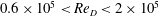 $0.6\times 10^{5}<Re_{D}<2\times 10^{5}$
, and, similar to figure 14 (for open-loop control), sample results are shown in figure 18. The representative shown parameters are the largest attainable stable attitude,
$0.6\times 10^{5}<Re_{D}<2\times 10^{5}$
, and, similar to figure 14 (for open-loop control), sample results are shown in figure 18. The representative shown parameters are the largest attainable stable attitude,
 $\bar{\unicode[STIX]{x1D6FC}}_{z\text{-}act}$
(figure 18
a), and attitude r.m.s. fluctuations,
$\bar{\unicode[STIX]{x1D6FC}}_{z\text{-}act}$
(figure 18
a), and attitude r.m.s. fluctuations,
 $\tilde{\unicode[STIX]{x1D6FC}}_{z\text{-}act}$
(figure 18
b), for stabilization about
$\tilde{\unicode[STIX]{x1D6FC}}_{z\text{-}act}$
(figure 18
b), for stabilization about
 $\unicode[STIX]{x1D6FC}_{z}=0^{\circ }$
(shown in green) and amplification (shown in red), where each is normalized by
$\unicode[STIX]{x1D6FC}_{z}=0^{\circ }$
(shown in green) and amplification (shown in red), where each is normalized by
 $\tilde{\unicode[STIX]{x1D6FC}}_{z\text{-}base}$
. These data show that the
$\tilde{\unicode[STIX]{x1D6FC}}_{z\text{-}base}$
. These data show that the
 $\bar{\unicode[STIX]{x1D6FC}}_{z\text{-}act}\approx 0.4\tilde{\unicode[STIX]{x1D6FC}}_{z\text{-}base}$
(or 30 % of the baseline amplitude) through the range of
$\bar{\unicode[STIX]{x1D6FC}}_{z\text{-}act}\approx 0.4\tilde{\unicode[STIX]{x1D6FC}}_{z\text{-}base}$
(or 30 % of the baseline amplitude) through the range of
 $Re_{D}$
, and since
$Re_{D}$
, and since
 $\tilde{\unicode[STIX]{x1D6FC}}_{z\text{-}base}$
increases linearly with flow speed (cf. figure 4
a) so does the attainable stable attitude. It is also shown that the r.m.s. attitude oscillations
$\tilde{\unicode[STIX]{x1D6FC}}_{z\text{-}base}$
increases linearly with flow speed (cf. figure 4
a) so does the attainable stable attitude. It is also shown that the r.m.s. attitude oscillations
 $\tilde{\unicode[STIX]{x1D6FC}}_{z\text{-}act}$
about
$\tilde{\unicode[STIX]{x1D6FC}}_{z\text{-}act}$
about
 $\unicode[STIX]{x1D6FC}_{z}=0^{\circ }$
(figure 18
b) are significantly suppressed from 50 % to 95 % for
$\unicode[STIX]{x1D6FC}_{z}=0^{\circ }$
(figure 18
b) are significantly suppressed from 50 % to 95 % for
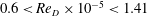 $0.6<Re_{D}\times 10^{-5}<1.41$
, indicating that the control authority of the actuation increases with
$0.6<Re_{D}\times 10^{-5}<1.41$
, indicating that the control authority of the actuation increases with
 $Re_{D}$
(although due to the fixed jet velocity the jet momentum decreases over this range:
$Re_{D}$
(although due to the fixed jet velocity the jet momentum decreases over this range:
 $12.8>C_{\unicode[STIX]{x1D707}}\times 10^{3}>2.0$
). However, similar to open-loop actuation (figure 14
b), the effectiveness of the stabilization diminishes somewhat for
$12.8>C_{\unicode[STIX]{x1D707}}\times 10^{3}>2.0$
). However, similar to open-loop actuation (figure 14
b), the effectiveness of the stabilization diminishes somewhat for
 $1.41<Re_{D}\times 10^{-5}<2$
(the suppression is approximately 85 %), owing to the maximum available actuation jet momentum in the present experiments not being sufficient at this flow speed (
$1.41<Re_{D}\times 10^{-5}<2$
(the suppression is approximately 85 %), owing to the maximum available actuation jet momentum in the present experiments not being sufficient at this flow speed (
 $C_{\unicode[STIX]{x1D707}}$
decreases to
$C_{\unicode[STIX]{x1D707}}$
decreases to
 $1.0\times 10^{-3}$
). These data suggest that the effectiveness of the actuation could be increased at higher
$1.0\times 10^{-3}$
). These data suggest that the effectiveness of the actuation could be increased at higher
 $C_{\unicode[STIX]{x1D707}}$
. The data in figure 18(b) also show that
$C_{\unicode[STIX]{x1D707}}$
. The data in figure 18(b) also show that
 $\tilde{\unicode[STIX]{x1D6FC}}_{z\text{-}act}$
can be monotonically amplified about
$\tilde{\unicode[STIX]{x1D6FC}}_{z\text{-}act}$
can be monotonically amplified about
 $\unicode[STIX]{x1D6FC}_{z}=0^{\circ }$
. In fact, for
$\unicode[STIX]{x1D6FC}_{z}=0^{\circ }$
. In fact, for
 $Re_{D}>1.14\times 10^{-5}$
, the model’s
$Re_{D}>1.14\times 10^{-5}$
, the model’s
 $\unicode[STIX]{x1D6FC}_{z}$
increases beyond the measurement range (approximately
$\unicode[STIX]{x1D6FC}_{z}$
increases beyond the measurement range (approximately
 $\pm 15^{\circ }$
, cf. § 2), although the trend indicates that for the higher flow speeds, closed-loop amplification can induce a limit cycle with motion having twice the attitude oscillations of the base flow.
$\pm 15^{\circ }$
, cf. § 2), although the trend indicates that for the higher flow speeds, closed-loop amplification can induce a limit cycle with motion having twice the attitude oscillations of the base flow.

Figure 19. Colour raster plots of the phase-averaged azimuthal vorticity concentrations
 $\hat{\unicode[STIX]{x1D701}}$
with overlaid velocity vectors in the near wake (at eight equal time increments
$\hat{\unicode[STIX]{x1D701}}$
with overlaid velocity vectors in the near wake (at eight equal time increments
 $0.125\unicode[STIX]{x1D70F}_{z}$
apart,
$0.125\unicode[STIX]{x1D70F}_{z}$
apart,
 $0<t/\unicode[STIX]{x1D70F}_{z\text{-}act}<0.875$
) in the presence of closed-loop control corresponding to figure 17(a–c): attitude stabilization about
$0<t/\unicode[STIX]{x1D70F}_{z\text{-}act}<0.875$
) in the presence of closed-loop control corresponding to figure 17(a–c): attitude stabilization about
 $\unicode[STIX]{x1D6FC}_{z}=0^{\circ }$
(
$\unicode[STIX]{x1D6FC}_{z}=0^{\circ }$
(
 $\unicode[STIX]{x1D70F}_{z\text{-}act}=\unicode[STIX]{x1D70F}_{z\text{-}0}^{\circ }=0.3\unicode[STIX]{x1D70F}_{z}$
, (a), and
$\unicode[STIX]{x1D70F}_{z\text{-}act}=\unicode[STIX]{x1D70F}_{z\text{-}0}^{\circ }=0.3\unicode[STIX]{x1D70F}_{z}$
, (a), and
 $2^{\circ }$
(
$2^{\circ }$
(
 $\unicode[STIX]{x1D70F}_{z\text{-}act}=\unicode[STIX]{x1D70F}_{z\text{-}2}^{\circ }=0.4\unicode[STIX]{x1D70F}_{z}$
, b), and oscillation amplification (
$\unicode[STIX]{x1D70F}_{z\text{-}act}=\unicode[STIX]{x1D70F}_{z\text{-}2}^{\circ }=0.4\unicode[STIX]{x1D70F}_{z}$
, b), and oscillation amplification (
 $\unicode[STIX]{x1D70F}_{z\text{-}act}=\unicode[STIX]{x1D70F}_{z\text{-}amplify}=1.25\unicode[STIX]{x1D70F}_{z}$
, (c)).
$\unicode[STIX]{x1D70F}_{z\text{-}act}=\unicode[STIX]{x1D70F}_{z\text{-}amplify}=1.25\unicode[STIX]{x1D70F}_{z}$
, (c)).
The effects of closed-loop actuation on the structure (and stability) of the near wake of the model (compared to the unactuated flow in figure 8) are depicted in colour raster plots of phase-averaged concentrations of azimuthal vorticity
 $\hat{\unicode[STIX]{x1D701}}$
superposed with distributions of velocity vectors in figure 19 (
$\hat{\unicode[STIX]{x1D701}}$
superposed with distributions of velocity vectors in figure 19 (
 $Re_{D}=1.15\times 10^{5}$
). Phase averaging is performed at equally spaced time intervals during the nominal period of the lateral motion limit cycle that are triggered by a laser vibrometer (cf. § 2), where the resulting closed-loop control limit-cycle periods are defined as
$Re_{D}=1.15\times 10^{5}$
). Phase averaging is performed at equally spaced time intervals during the nominal period of the lateral motion limit cycle that are triggered by a laser vibrometer (cf. § 2), where the resulting closed-loop control limit-cycle periods are defined as
 $\unicode[STIX]{x1D70F}_{z\text{-}0^{\circ }}$
,
$\unicode[STIX]{x1D70F}_{z\text{-}0^{\circ }}$
,
 $\unicode[STIX]{x1D70F}_{z\text{-}2^{\circ }}$
, and
$\unicode[STIX]{x1D70F}_{z\text{-}2^{\circ }}$
, and
 $\unicode[STIX]{x1D70F}_{z\text{-}amplify}$
, respectively. When the model is stabilized about
$\unicode[STIX]{x1D70F}_{z\text{-}amplify}$
, respectively. When the model is stabilized about
 $\unicode[STIX]{x1D6FC}_{z}=0^{\circ }$
(figure 19
a,
$\unicode[STIX]{x1D6FC}_{z}=0^{\circ }$
(figure 19
a,
 $\unicode[STIX]{x1D70F}_{z\text{-}0^{\circ }}=0.3\unicode[STIX]{x1D70F}_{z}$
or approximately
$\unicode[STIX]{x1D70F}_{z\text{-}0^{\circ }}=0.3\unicode[STIX]{x1D70F}_{z}$
or approximately
 $20\unicode[STIX]{x1D70F}_{conv}$
) the actuation-induced aerodynamic loads oppose the motion of the model so that Act1 (top) and Act2 (bottom) are activated when the model moves CW (figure 19
a4–6) and CCW (figure 19
a1,2,8), respectively. As a result of the actuation, the segment of the separating azimuthal shear layer that is adjacent to the jet becomes partially attached to the tail section and is deflected towards the centre of the wake. Because this deflection occurs over a finite segment, it leads to a localized streamwise depression of the azimuthal vorticity concentrations and thereby to streamwise tilting near the edges of the forced segment. Although these 3D vortical structures were not investigated in detail, it is conjectured that the alternating time-periodic actuation on each side (top and bottom) of the wake leads to the formation of ring-like vortical structures. Similarly, when the model’s attitude is stabilized about
$20\unicode[STIX]{x1D70F}_{conv}$
) the actuation-induced aerodynamic loads oppose the motion of the model so that Act1 (top) and Act2 (bottom) are activated when the model moves CW (figure 19
a4–6) and CCW (figure 19
a1,2,8), respectively. As a result of the actuation, the segment of the separating azimuthal shear layer that is adjacent to the jet becomes partially attached to the tail section and is deflected towards the centre of the wake. Because this deflection occurs over a finite segment, it leads to a localized streamwise depression of the azimuthal vorticity concentrations and thereby to streamwise tilting near the edges of the forced segment. Although these 3D vortical structures were not investigated in detail, it is conjectured that the alternating time-periodic actuation on each side (top and bottom) of the wake leads to the formation of ring-like vortical structures. Similarly, when the model’s attitude is stabilized about
 $\unicode[STIX]{x1D6FC}_{z}=2^{\circ }$
(figure 19(b),
$\unicode[STIX]{x1D6FC}_{z}=2^{\circ }$
(figure 19(b),
 $\unicode[STIX]{x1D70F}_{z\text{-}2^{\circ }}=0.4\unicode[STIX]{x1D70F}_{z}$
or approximately
$\unicode[STIX]{x1D70F}_{z\text{-}2^{\circ }}=0.4\unicode[STIX]{x1D70F}_{z}$
or approximately
 $30\unicode[STIX]{x1D70F}_{conv}$
), only Act1 is activated and the deflection of the separating shear layer towards the centre of the wake is more pronounced. By comparison to the base flow in figure 8(c), both actuation programs clearly stabilize the large-scale lateral oscillations of the near wake, although the azimuthally non-uniform effects of the actuation clearly alter its structure compared to the wake of a stationary model. The actuation can certainly accentuate the oscillations of the free-yawing model and significantly enhance its yaw rate, as depicted in figure 19(c) (
$30\unicode[STIX]{x1D70F}_{conv}$
), only Act1 is activated and the deflection of the separating shear layer towards the centre of the wake is more pronounced. By comparison to the base flow in figure 8(c), both actuation programs clearly stabilize the large-scale lateral oscillations of the near wake, although the azimuthally non-uniform effects of the actuation clearly alter its structure compared to the wake of a stationary model. The actuation can certainly accentuate the oscillations of the free-yawing model and significantly enhance its yaw rate, as depicted in figure 19(c) (
 $\unicode[STIX]{x1D70F}_{z\text{-}amplify}=1.25\unicode[STIX]{x1D70F}_{z}$
or approximately
$\unicode[STIX]{x1D70F}_{z\text{-}amplify}=1.25\unicode[STIX]{x1D70F}_{z}$
or approximately
 $90\unicode[STIX]{x1D70F}_{conv}$
) when the model is moving CCW (figure 19
c1,2,8) and CW (figure 19
c4–6). It is remarkable that during the peak of the actuation (figure 19
c3,7), the forced shear layer segments become fully attached to the aft end of the body, forming a momentary domain of trapped vorticity that is bounded on the opposite end by vorticity of the opposite sense. As shown in figure 8(b3,7), during these deflections the centre plane of the near wake is momentarily dominated by the cross-stream velocity distribution that is deflected in the streamwise direction by the shear layer on the opposite surface.
$90\unicode[STIX]{x1D70F}_{conv}$
) when the model is moving CCW (figure 19
c1,2,8) and CW (figure 19
c4–6). It is remarkable that during the peak of the actuation (figure 19
c3,7), the forced shear layer segments become fully attached to the aft end of the body, forming a momentary domain of trapped vorticity that is bounded on the opposite end by vorticity of the opposite sense. As shown in figure 8(b3,7), during these deflections the centre plane of the near wake is momentarily dominated by the cross-stream velocity distribution that is deflected in the streamwise direction by the shear layer on the opposite surface.

Figure 20. Colour raster plots of
 $\text{d}\hat{M}_{xyz}$
(
$\text{d}\hat{M}_{xyz}$
(
 $y,t\mid x=1.8D$
) in (a–c) and of
$y,t\mid x=1.8D$
) in (a–c) and of
 $\text{d}\hat{M}_{xz}(x,t)$
in (d–f); (a,d), (b,e), and (c,f) correspond to the actuation programs in figure 19(a–c), respectively.
$\text{d}\hat{M}_{xz}(x,t)$
in (d–f); (a,d), (b,e), and (c,f) correspond to the actuation programs in figure 19(a–c), respectively.
The alteration of the coupling between the model and its near wake by the actuation is analysed by computing the contribution to the aerodynamic moment from vorticity concentrations (cf. figure 9). Figure 20(a–c) show colour raster plots of
 $\text{d}\hat{M}_{xyz}$
(
$\text{d}\hat{M}_{xyz}$
(
 $y,t$
) at
$y,t$
) at
 $x/D=1.8$
in the meridional
$x/D=1.8$
in the meridional
 $x$
–
$x$
–
 $y$
measurement plane for each of the closed-loop actuation programs in figure 19(a–c), and the corresponding raster plots of
$y$
measurement plane for each of the closed-loop actuation programs in figure 19(a–c), and the corresponding raster plots of
 $\text{d}\hat{M}_{xz}(x,t)$
(integrated in
$\text{d}\hat{M}_{xz}(x,t)$
(integrated in
 $y$
) are shown in figure 20(d–f) (these moment contributions are calculated using (3.8), § 3). When the model (and the near wake) are stabilized (
$y$
) are shown in figure 20(d–f) (these moment contributions are calculated using (3.8), § 3). When the model (and the near wake) are stabilized (
 $\unicode[STIX]{x1D6FC}_{z}=0^{\circ }$
and
$\unicode[STIX]{x1D6FC}_{z}=0^{\circ }$
and
 $2^{\circ }$
, figure 19
a,b) the integral measure of the contributions to the induced moment (at
$2^{\circ }$
, figure 19
a,b) the integral measure of the contributions to the induced moment (at
 $x/D=1.8$
) from vorticity concentrations within the separating shear layers is nearly time-invariant, indicating that the actuation-induced aerodynamic loads nearly balance the loads on the free-yawing model (cf. figure 9). In contrast to figure 9(c), figure 20(d) exhibits only mild streamwise and temporal variations during the entire limit cycle of the model’s oscillations despite the fact that both actuators are active in alternation. However, when the model is stabilized about an offset attitude (
$x/D=1.8$
) from vorticity concentrations within the separating shear layers is nearly time-invariant, indicating that the actuation-induced aerodynamic loads nearly balance the loads on the free-yawing model (cf. figure 9). In contrast to figure 9(c), figure 20(d) exhibits only mild streamwise and temporal variations during the entire limit cycle of the model’s oscillations despite the fact that both actuators are active in alternation. However, when the model is stabilized about an offset attitude (
 $\unicode[STIX]{x1D6FC}_{z}=2^{\circ }$
, figure 20
e), the wake contributes to a CW moment near the aft surface during the entire cycle and to a CCW moment within the domain
$\unicode[STIX]{x1D6FC}_{z}=2^{\circ }$
, figure 20
e), the wake contributes to a CW moment near the aft surface during the entire cycle and to a CCW moment within the domain
 $1.8<x/D<2.2$
during
$1.8<x/D<2.2$
during
 $0.4<t/\unicode[STIX]{x1D70F}_{z}<0.9$
(which is apparently a slightly delayed effect relative to the onset of actuation at
$0.4<t/\unicode[STIX]{x1D70F}_{z}<0.9$
(which is apparently a slightly delayed effect relative to the onset of actuation at
 $t/\unicode[STIX]{x1D70F}_{z}\approx 0.25$
). The larger moment magnitude in the wake during stabilization about
$t/\unicode[STIX]{x1D70F}_{z}\approx 0.25$
). The larger moment magnitude in the wake during stabilization about
 $\unicode[STIX]{x1D6FC}_{z}=2^{\circ }$
compared to
$\unicode[STIX]{x1D6FC}_{z}=2^{\circ }$
compared to
 $\unicode[STIX]{x1D6FC}_{z}=0^{\circ }$
(figure 20
e,d) is due to the larger fluctuations of the model about its new equilibrium point (from
$\unicode[STIX]{x1D6FC}_{z}=0^{\circ }$
(figure 20
e,d) is due to the larger fluctuations of the model about its new equilibrium point (from
 $0.4^{\circ }$
to
$0.4^{\circ }$
to
 $0.6^{\circ }$
, as shown in figure 15). The amplification actuation strongly accentuates the effects of the aerodynamic restoring moments, where the lateral extrema associated with the alternating attachment of the opposite segments of the forced shear layer to the base of the model (figure 19
c3,7) are shown in figure 20(c) (in comparison to figure 9(a) of the base flow). The resulting cross-flow integrated moment
$0.6^{\circ }$
, as shown in figure 15). The amplification actuation strongly accentuates the effects of the aerodynamic restoring moments, where the lateral extrema associated with the alternating attachment of the opposite segments of the forced shear layer to the base of the model (figure 19
c3,7) are shown in figure 20(c) (in comparison to figure 9(a) of the base flow). The resulting cross-flow integrated moment
 $\text{d}\hat{M}_{xz}$
(figure 20
f) exhibits a significant increase during the two halves of the oscillation cycle both near the aft end of the model (
$\text{d}\hat{M}_{xz}$
(figure 20
f) exhibits a significant increase during the two halves of the oscillation cycle both near the aft end of the model (
 $x/D<1.4$
) and farther downstream (
$x/D<1.4$
) and farther downstream (
 $1.45<x/D<2$
). The sense of these contributions is reversed during each half of the cycle so that
$1.45<x/D<2$
). The sense of these contributions is reversed during each half of the cycle so that
 $\text{d}\hat{M}_{xz}$
in
$\text{d}\hat{M}_{xz}$
in
 $x/D<1.4$
and
$x/D<1.4$
and
 $1.45<x/D<2$
are opposite and coincide with the model’s rotation. The times at which the peaks occur (maximum at
$1.45<x/D<2$
are opposite and coincide with the model’s rotation. The times at which the peaks occur (maximum at
 $0.3\unicode[STIX]{x1D70F}_{z}$
and minimum
$0.3\unicode[STIX]{x1D70F}_{z}$
and minimum
 $0.8\unicode[STIX]{x1D70F}_{z}$
) correspond to a
$0.8\unicode[STIX]{x1D70F}_{z}$
) correspond to a
 $20^{\circ }$
phase lag of the moments with respect to the model’s attitude, which is in agreement with the phase lag of
$20^{\circ }$
phase lag of the moments with respect to the model’s attitude, which is in agreement with the phase lag of
 $C_{Y}$
(figure 17
c3). In contrast to the unactuated model oscillation, for which the wake contribution is mostly out of phase with the model’s motion (figure 9
c), during closed-loop amplification the wake contribution is mostly in phase with the motion of the model and therefore provides a destabilizing moment during
$C_{Y}$
(figure 17
c3). In contrast to the unactuated model oscillation, for which the wake contribution is mostly out of phase with the model’s motion (figure 9
c), during closed-loop amplification the wake contribution is mostly in phase with the motion of the model and therefore provides a destabilizing moment during
 $0.2<t/\unicode[STIX]{x1D70F}_{z}<0.4$
and
$0.2<t/\unicode[STIX]{x1D70F}_{z}<0.4$
and
 $0.7<t/\unicode[STIX]{x1D70F}_{z}<0.9$
. The data in figure 20(d–f) indicate that the changes in the model limit cycle during stabilization and amplification (cf. figure 17) are not only in agreement with velocity measurements in the near wake, but that the velocity field may be used to estimate the locations and times within the near wake at which the stabilizing and destabilizing effects are induced.
$0.7<t/\unicode[STIX]{x1D70F}_{z}<0.9$
. The data in figure 20(d–f) indicate that the changes in the model limit cycle during stabilization and amplification (cf. figure 17) are not only in agreement with velocity measurements in the near wake, but that the velocity field may be used to estimate the locations and times within the near wake at which the stabilizing and destabilizing effects are induced.
6 Concluding remarks
The reciprocal coupling between a free-yawing axisymmetric bluff body and its near wake is manipulated in wind tunnel experiments to modify the flow-induced loads for directional control. These loads are controlled indirectly through prescribed modification of the near-wake flow by exploiting the receptivity of the aft-separating shear layer to weak pulsed fluidic actuation effected by two diametrically opposed and independently controlled synthetic jet actuators.
In the absence of wake control, the coupled interactions of the free-yawing wire-mounted body with the cross-flow result in nominally time-periodic yaw oscillations that are sustained by the balance between the lateral inertia and unsteady flow-induced restoring loads over the body where the oscillation period
 $\unicode[STIX]{x1D70F}_{z}$
depends on the body’s geometry (including rotation axis) and moment of inertia. This motion is modelled as a second-order system having time-dependent natural frequency
$\unicode[STIX]{x1D70F}_{z}$
depends on the body’s geometry (including rotation axis) and moment of inertia. This motion is modelled as a second-order system having time-dependent natural frequency
 $\unicode[STIX]{x1D714}_{n}(t)$
and damping ratio
$\unicode[STIX]{x1D714}_{n}(t)$
and damping ratio
 $\unicode[STIX]{x1D709}(t)$
, that is used to estimate the flow loads on the moving body by evaluating the temporal variation of
$\unicode[STIX]{x1D709}(t)$
, that is used to estimate the flow loads on the moving body by evaluating the temporal variation of
 $\unicode[STIX]{x1D714}_{n}$
and
$\unicode[STIX]{x1D714}_{n}$
and
 $\unicode[STIX]{x1D709}$
in wind tunnel experiments. Phase-locked PIV measurements in the body’s meridional plane demonstrate that as the body oscillates the near wake is deflected laterally opposite to the sense of rotation, and commensurate with the alternating sense of the restoring flow-induced yaw moment. It is also shown that the dominant oscillation amplitude and frequency increase monotonically with Reynolds number.
$\unicode[STIX]{x1D709}$
in wind tunnel experiments. Phase-locked PIV measurements in the body’s meridional plane demonstrate that as the body oscillates the near wake is deflected laterally opposite to the sense of rotation, and commensurate with the alternating sense of the restoring flow-induced yaw moment. It is also shown that the dominant oscillation amplitude and frequency increase monotonically with Reynolds number.
That the characteristic period and frequency of the oscillatory motion are respectively significantly longer and lower than the convective time scale and shedding frequency of vorticity concentrations into the near wake indicates that the motion of the body and hence its attitude can be altered on time scales that are significantly shorter than the nominal lateral oscillation period. In fact, a central objective of the present investigations was to demonstrate that the free-body dynamics can be effectively controlled through fluid mechanical manipulation of the near wake despite the significant disparity between the time scale of the body motion and the convective time scale of its near wake.
The interactions between the body and the cross-flow over the aft tail surface and therefore its natural lateral yawing oscillations are manipulated by affecting the fluid mechanics of the near wake using transitory attachment of azimuthal segments of the separated shear layer on opposite ends of the aft tail segments centred about the plane of the body yawing motion. Actuation is effected by low-amplitude fluidic perturbations using bursts of brief momentum pulses of two opposite synthetic jets (
 $\unicode[STIX]{x1D70F}_{act}\approx 0.0016\unicode[STIX]{x1D70F}_{z}$
) that by themselves cannot affect the body’s motion. The present investigations demonstrated that when either jet produces anywhere from even a single pulse to multiple successive actuation pulses during a fraction of the body’s lateral oscillations period, the transitory coupling between the actuation and the flow in the near wake cumulatively alters the wake dynamics and the yawing moment. Longer actuation bursts (within
$\unicode[STIX]{x1D70F}_{act}\approx 0.0016\unicode[STIX]{x1D70F}_{z}$
) that by themselves cannot affect the body’s motion. The present investigations demonstrated that when either jet produces anywhere from even a single pulse to multiple successive actuation pulses during a fraction of the body’s lateral oscillations period, the transitory coupling between the actuation and the flow in the near wake cumulatively alters the wake dynamics and the yawing moment. Longer actuation bursts (within
 $100\unicode[STIX]{x1D70F}_{conv}$
) can be used to achieve desired proportional control of the flow-induced loads sufficient to alter the body’s yawing trajectory. Measurements of the jet’s consecutive pulses with the separating shear layer show the formation of trains of small-scale vortices that apparently alter entrainment into the adjacent separating shear layer to deflect it and the outer flow towards the inner wake. Depending on the instantaneous direction of rotation and attitude of the body, the resulting transitory side force and yawing moment either support or resist the lateral oscillatory motion and act to increase or decrease its azimuthal yawing angle and thereby amplify or attenuate the amplitude of the lateral oscillations. It is noteworthy that the response of the motion following the termination of the actuation is inherently slower owing to the slow relaxation of the separated flow on the aft end of the body (it takes 4–5 oscillation cycles for the time-averaged attitude and oscillation amplitude to return to the nominal levels in the absence of actuation).
$100\unicode[STIX]{x1D70F}_{conv}$
) can be used to achieve desired proportional control of the flow-induced loads sufficient to alter the body’s yawing trajectory. Measurements of the jet’s consecutive pulses with the separating shear layer show the formation of trains of small-scale vortices that apparently alter entrainment into the adjacent separating shear layer to deflect it and the outer flow towards the inner wake. Depending on the instantaneous direction of rotation and attitude of the body, the resulting transitory side force and yawing moment either support or resist the lateral oscillatory motion and act to increase or decrease its azimuthal yawing angle and thereby amplify or attenuate the amplitude of the lateral oscillations. It is noteworthy that the response of the motion following the termination of the actuation is inherently slower owing to the slow relaxation of the separated flow on the aft end of the body (it takes 4–5 oscillation cycles for the time-averaged attitude and oscillation amplitude to return to the nominal levels in the absence of actuation).
Bi-directional flow-induced loads that can affect the lateral attitude and motion of the body using strategically timed actuation during the oscillation cycle can be implemented using feedback control. To this end, a PID closed-loop controller was developed and implemented to command desired attitude and motion trajectories by using the measured attitude as feedback and effecting desired bursts of jet pulses. Control was demonstrated by effecting prescribed, stabilized attitudes (centre and offset about
 $0^{\circ }$
and
$0^{\circ }$
and
 $2^{\circ }$
, respectively), and by deliberate amplification of the base flow oscillations. Time traces of the body’s attitude during PID control demonstrate that the controller stabilizes the body about the desired attitude angles within approximately 2–3 lateral oscillation cycles (the stabilization time increases for offset attitude) and that the oscillation amplitude is significantly reduced (
$2^{\circ }$
, respectively), and by deliberate amplification of the base flow oscillations. Time traces of the body’s attitude during PID control demonstrate that the controller stabilizes the body about the desired attitude angles within approximately 2–3 lateral oscillation cycles (the stabilization time increases for offset attitude) and that the oscillation amplitude is significantly reduced (
 $\unicode[STIX]{x1D6FC}_{z,rms}$
decreases by up to 90 %) while the lateral oscillation frequency increases by an approximate factor of three. Accompanying PIV measurements in the near wake show that by comparison to the base flow, attitude control significantly stabilizes the large-scale lateral oscillations of the near wake, although azimuthally non-uniform effects of the actuation alter its structure compared to the wake of a stationary body. The present investigations also showed that while centre stabilization is implemented using both opposite aft actuators, offset attitude can be accomplished using only a single aft actuator to balance the restoring yawing moment of the base flow. The controller can also effectively destabilize or amplify the base oscillations of the body (
$\unicode[STIX]{x1D6FC}_{z,rms}$
decreases by up to 90 %) while the lateral oscillation frequency increases by an approximate factor of three. Accompanying PIV measurements in the near wake show that by comparison to the base flow, attitude control significantly stabilizes the large-scale lateral oscillations of the near wake, although azimuthally non-uniform effects of the actuation alter its structure compared to the wake of a stationary body. The present investigations also showed that while centre stabilization is implemented using both opposite aft actuators, offset attitude can be accomplished using only a single aft actuator to balance the restoring yawing moment of the base flow. The controller can also effectively destabilize or amplify the base oscillations of the body (
 $\unicode[STIX]{x1D6FC}_{z,rms}$
increases by approximately 175 %) with similar onset and relaxation times as for attitude stabilization by alternating activation of the aft actuators to induce yawing moments that support the motion and increase the excursion amplitude.
$\unicode[STIX]{x1D6FC}_{z,rms}$
increases by approximately 175 %) with similar onset and relaxation times as for attitude stabilization by alternating activation of the aft actuators to induce yawing moments that support the motion and increase the excursion amplitude.
Finally, although the range of Reynolds number explored in the present investigation was somewhat limited (
 $0.6<Re_{D}\times 10^{-5}<2$
), the present findings indicate that the range of stable offset attitude angles that can be effected and sustained is nearly an invariant fraction (approximately 0.3) of the base motion attitude excursion. Because the amplitude of the lateral oscillations of the base motion increases nearly linearly with
$0.6<Re_{D}\times 10^{-5}<2$
), the present findings indicate that the range of stable offset attitude angles that can be effected and sustained is nearly an invariant fraction (approximately 0.3) of the base motion attitude excursion. Because the amplitude of the lateral oscillations of the base motion increases nearly linearly with
 $Re_{D}$
, the range of stable offset attitude angles that can be effected by closed-loop control (for a given
$Re_{D}$
, the range of stable offset attitude angles that can be effected by closed-loop control (for a given
 $C_{\unicode[STIX]{x1D707}}$
) also increases. Therefore, even though the increase in control effectiveness with
$C_{\unicode[STIX]{x1D707}}$
) also increases. Therefore, even though the increase in control effectiveness with
 $Re_{D}$
in the present investigations was limited by the performance of the actuators, these findings indicate that similar control authority may be attained at considerably higher Reynolds numbers.
$Re_{D}$
in the present investigations was limited by the performance of the actuators, these findings indicate that similar control authority may be attained at considerably higher Reynolds numbers.
Acknowledgements
This work was supported by the Army Research Office (monitored by Dr M. Munson).
Appendix. PID controller design
The PID controller for closed-loop attitude control is shown in figure 21. This type of controller was selected based on the results of cumulative actuation effect of open-loop pulsed actuation (cf. § 4), along with effective modelling of the baseline dynamics using a second-order, linear time-varying system (§ 3).

Figure 21. Schematic diagram of the closed-loop PID controller.
The controller uses the difference between the desired (goal) outputs
 $\unicode[STIX]{x1D6FC}_{goal}$
and
$\unicode[STIX]{x1D6FC}_{goal}$
and
 $\dot{\unicode[STIX]{x1D6FC}}_{goal}$
, and the sensor (vibrometer) inputs
$\dot{\unicode[STIX]{x1D6FC}}_{goal}$
, and the sensor (vibrometer) inputs
 $\unicode[STIX]{x1D6FC}_{z}$
and
$\unicode[STIX]{x1D6FC}_{z}$
and
 $\dot{\unicode[STIX]{x1D6FC}_{z}}$
, as proportional and derivative errors
$\dot{\unicode[STIX]{x1D6FC}_{z}}$
, as proportional and derivative errors
 $e_{p}=\unicode[STIX]{x1D6FC}_{goal}-\unicode[STIX]{x1D6FC}_{z}$
and
$e_{p}=\unicode[STIX]{x1D6FC}_{goal}-\unicode[STIX]{x1D6FC}_{z}$
and
 $e_{D}=\dot{\unicode[STIX]{x1D6FC}}_{goal}-\dot{\unicode[STIX]{x1D6FC}_{z}}$
and numerical integration of the proportional error to compute the integral error
$e_{D}=\dot{\unicode[STIX]{x1D6FC}}_{goal}-\dot{\unicode[STIX]{x1D6FC}_{z}}$
and numerical integration of the proportional error to compute the integral error
 $e_{I}$
(as noted in § 2, the uncertainties in the measured angle and rate are
$e_{I}$
(as noted in § 2, the uncertainties in the measured angle and rate are
 $\pm 0.16~\text{mm}$
and
$\pm 0.16~\text{mm}$
and
 $\pm 2~\text{mm}~\text{s}^{-1}$
, respectively).
$\pm 2~\text{mm}~\text{s}^{-1}$
, respectively).
When the controller is initiated, the opposing actuator jets (Act1, Act2) are each driven at some initial state amplitude modulation of their resonant waveforms (cf. § 2) in the absence of control signal. The command signal is then added to and subtracted from the initial states of Act1 and Act2, respectively, to account for their opposite orientations. The relative amplitudes of the jets are scaled by
 $C_{1}$
and
$C_{1}$
and
 $C_{2}$
to correct for their relative strength (100 % modulation corresponds jet momentum coefficient
$C_{2}$
to correct for their relative strength (100 % modulation corresponds jet momentum coefficient
 $C_{\unicode[STIX]{x1D707}}=0.003$
). Each of the two command signals is passed through a saturation element and sent to an external function generator and amplifier to form an amplitude-modulated resonance waveform. The controller’s bandwidth is limited primarily by the rate at which the yawing moment
$C_{\unicode[STIX]{x1D707}}=0.003$
). Each of the two command signals is passed through a saturation element and sent to an external function generator and amplifier to form an amplitude-modulated resonance waveform. The controller’s bandwidth is limited primarily by the rate at which the yawing moment
 $C_{Y}$
is induced, nominally 0.01 per
$C_{Y}$
is induced, nominally 0.01 per
 $2\unicode[STIX]{x1D70F}_{conv}$
, leading to a
$2\unicode[STIX]{x1D70F}_{conv}$
, leading to a
 $-3~\text{dB}$
point bandwidth of
$-3~\text{dB}$
point bandwidth of
 $24.1(Re_{D}/1.15\times 10^{5})$
Hz (accounting for the effects of the free-stream speed).
$24.1(Re_{D}/1.15\times 10^{5})$
Hz (accounting for the effects of the free-stream speed).

Figure 22. Determination of PID control coefficients
 $\unicode[STIX]{x1D705}_{D}$
,
$\unicode[STIX]{x1D705}_{D}$
,
 $\unicode[STIX]{x1D705}_{I}$
, and
$\unicode[STIX]{x1D705}_{I}$
, and
 $\unicode[STIX]{x1D705}_{P}$
when the model is stabilized at
$\unicode[STIX]{x1D705}_{P}$
when the model is stabilized at
 $\unicode[STIX]{x1D6FC}_{z}=0^{\circ }$
(
$\unicode[STIX]{x1D6FC}_{z}=0^{\circ }$
(
 $Re_{D}=1.73\times 10^{5}$
,
$Re_{D}=1.73\times 10^{5}$
,
 $C_{\unicode[STIX]{x1D707}}=0.003$
) by varying: (a)
$C_{\unicode[STIX]{x1D707}}=0.003$
) by varying: (a)
 $\unicode[STIX]{x1D705}_{D}$
with
$\unicode[STIX]{x1D705}_{D}$
with
 $\unicode[STIX]{x1D705}_{I}=\unicode[STIX]{x1D705}_{P}=0$
; (b)
$\unicode[STIX]{x1D705}_{I}=\unicode[STIX]{x1D705}_{P}=0$
; (b)
 $\unicode[STIX]{x1D705}_{P}$
with
$\unicode[STIX]{x1D705}_{P}$
with
 $\unicode[STIX]{x1D705}_{D}=40\,\%/(\text{deg.}~\text{s}^{-1})$
and
$\unicode[STIX]{x1D705}_{D}=40\,\%/(\text{deg.}~\text{s}^{-1})$
and
 $\unicode[STIX]{x1D705}_{I}=0$
; and (c)
$\unicode[STIX]{x1D705}_{I}=0$
; and (c)
 $\unicode[STIX]{x1D705}_{I}$
with
$\unicode[STIX]{x1D705}_{I}$
with
 $\unicode[STIX]{x1D705}_{D}=40\,\%/(\text{deg.}~\text{s}^{-1})$
and
$\unicode[STIX]{x1D705}_{D}=40\,\%/(\text{deg.}~\text{s}^{-1})$
and
 $\unicode[STIX]{x1D705}_{P}=1.5\,\%/\text{deg.}$
The operational parameters
$\unicode[STIX]{x1D705}_{P}=1.5\,\%/\text{deg.}$
The operational parameters
 $\unicode[STIX]{x1D705}_{Do}$
,
$\unicode[STIX]{x1D705}_{Do}$
,
 $\unicode[STIX]{x1D705}_{Io}$
, and
$\unicode[STIX]{x1D705}_{Io}$
, and
 $\unicode[STIX]{x1D705}_{Po}$
are marked by dashed lines.
$\unicode[STIX]{x1D705}_{Po}$
are marked by dashed lines.
The PID control coefficients are determined iteratively when the model is stabilized at an attitude of
 $\unicode[STIX]{x1D6FC}_{z}=0^{\circ }$
at
$\unicode[STIX]{x1D6FC}_{z}=0^{\circ }$
at
 $Re_{D}=1.73\times 10^{5}$
, and the same controller is used over the full range of
$Re_{D}=1.73\times 10^{5}$
, and the same controller is used over the full range of
 $Re_{D}$
. The effectiveness of the coefficients is assessed by computing the r.m.s. attitude
$Re_{D}$
. The effectiveness of the coefficients is assessed by computing the r.m.s. attitude
 $\unicode[STIX]{x1D6FC}_{z,rms}$
(in the absence of control
$\unicode[STIX]{x1D6FC}_{z,rms}$
(in the absence of control
 $\unicode[STIX]{x1D6FC}_{z,rms}\approx 6.5^{\circ }$
). Initial alteration of these coefficients revealed that control was most sensitive to the coefficient
$\unicode[STIX]{x1D6FC}_{z,rms}\approx 6.5^{\circ }$
). Initial alteration of these coefficients revealed that control was most sensitive to the coefficient
 $\unicode[STIX]{x1D705}_{D}$
, and this coefficient was varied when
$\unicode[STIX]{x1D705}_{D}$
, and this coefficient was varied when
 $\unicode[STIX]{x1D705}_{P}=\unicode[STIX]{x1D705}_{I}=0$
. As shown in figure 22(a), for
$\unicode[STIX]{x1D705}_{P}=\unicode[STIX]{x1D705}_{I}=0$
. As shown in figure 22(a), for
 $\unicode[STIX]{x1D705}_{D}<0$
,
$\unicode[STIX]{x1D705}_{D}<0$
,
 $\unicode[STIX]{x1D6FC}_{z,rms}$
increased significantly, yielding a controller that acted as a negative aerodynamic damper, while for
$\unicode[STIX]{x1D6FC}_{z,rms}$
increased significantly, yielding a controller that acted as a negative aerodynamic damper, while for
 $\unicode[STIX]{x1D705}_{D}<0,\unicode[STIX]{x1D6FC}_{z,rms}$
quickly diminished to an asymptotic value of
$\unicode[STIX]{x1D705}_{D}<0,\unicode[STIX]{x1D6FC}_{z,rms}$
quickly diminished to an asymptotic value of
 $0.48^{\circ }$
for
$0.48^{\circ }$
for
 $\unicode[STIX]{x1D705}_{D}>10(\%/\text{deg}~\text{s}^{-1})$
, and so
$\unicode[STIX]{x1D705}_{D}>10(\%/\text{deg}~\text{s}^{-1})$
, and so
 $\unicode[STIX]{x1D705}_{D}$
is selected to be
$\unicode[STIX]{x1D705}_{D}$
is selected to be
 $\unicode[STIX]{x1D705}_{Do}=40(\%/\text{deg}~\text{s}^{-1})$
. Figure 22(b) shows that
$\unicode[STIX]{x1D705}_{Do}=40(\%/\text{deg}~\text{s}^{-1})$
. Figure 22(b) shows that
 $\unicode[STIX]{x1D6FC}_{z,rms}$
is less sensitive to
$\unicode[STIX]{x1D6FC}_{z,rms}$
is less sensitive to
 $\unicode[STIX]{x1D705}_{P}$
(for
$\unicode[STIX]{x1D705}_{P}$
(for
 $\unicode[STIX]{x1D705}_{D}=\unicode[STIX]{x1D705}_{Do}$
and
$\unicode[STIX]{x1D705}_{D}=\unicode[STIX]{x1D705}_{Do}$
and
 $\unicode[STIX]{x1D705}_{I}=0$
) with a minimum
$\unicode[STIX]{x1D705}_{I}=0$
) with a minimum
 $\unicode[STIX]{x1D6FC}_{z,rms}=0.43^{\circ }$
at
$\unicode[STIX]{x1D6FC}_{z,rms}=0.43^{\circ }$
at
 $\unicode[STIX]{x1D705}_{Po}=1.5(\%/\text{deg})$
. Finally, as shown in figure 22(c), variation of
$\unicode[STIX]{x1D705}_{Po}=1.5(\%/\text{deg})$
. Finally, as shown in figure 22(c), variation of
 $\unicode[STIX]{x1D705}_{I}$
with fixed
$\unicode[STIX]{x1D705}_{I}$
with fixed
 $\unicode[STIX]{x1D705}_{Do}$
and
$\unicode[STIX]{x1D705}_{Do}$
and
 $\unicode[STIX]{x1D705}_{Po}$
yields a minimum
$\unicode[STIX]{x1D705}_{Po}$
yields a minimum
 $\unicode[STIX]{x1D6FC}_{z,rms}=0.40^{\circ }$
at
$\unicode[STIX]{x1D6FC}_{z,rms}=0.40^{\circ }$
at
 $\unicode[STIX]{x1D705}_{Io}=75(\%/\text{deg}~\text{s}^{-1})$
. These PID coefficients (
$\unicode[STIX]{x1D705}_{Io}=75(\%/\text{deg}~\text{s}^{-1})$
. These PID coefficients (
 $\unicode[STIX]{x1D705}_{Do}$
,
$\unicode[STIX]{x1D705}_{Do}$
,
 $\unicode[STIX]{x1D705}_{Po}$
, and
$\unicode[STIX]{x1D705}_{Po}$
, and
 $\unicode[STIX]{x1D705}_{Io}$
) are used for all the results presented in § 5. For the three control programs in § 5 the coefficients
$\unicode[STIX]{x1D705}_{Io}$
) are used for all the results presented in § 5. For the three control programs in § 5 the coefficients
 $C_{1}$
and
$C_{1}$
and
 $C_{2}$
are set as follows: attitude about
$C_{2}$
are set as follows: attitude about
 $\unicode[STIX]{x1D6FC}_{z}=0^{\circ }$
:
$\unicode[STIX]{x1D6FC}_{z}=0^{\circ }$
:
 $C_{1}\sim C_{2}\sim 1$
, offset attitude
$C_{1}\sim C_{2}\sim 1$
, offset attitude
 $\unicode[STIX]{x1D6FC}_{z}=2^{\circ }$
:
$\unicode[STIX]{x1D6FC}_{z}=2^{\circ }$
:
 $C_{1}=1$
,
$C_{1}=1$
,
 $C_{2}=0$
, and oscillation amplification about
$C_{2}=0$
, and oscillation amplification about
 $\unicode[STIX]{x1D6FC}_{z}=0^{\circ }$
:
$\unicode[STIX]{x1D6FC}_{z}=0^{\circ }$
:
 $C_{1}$
and
$C_{1}$
and
 $C_{2}$
inverted from suppression about
$C_{2}$
inverted from suppression about
 $0^{\circ }$
. It is also noted that the initial triggering condition of this controller is generally set to
$0^{\circ }$
. It is also noted that the initial triggering condition of this controller is generally set to
 $3^{\circ }$
in § 5, where this starting angle did not significantly affect the controlled response of the model and was only chosen to match the results shown in the open-loop section (§ 4), where initial conditions were significant.
$3^{\circ }$
in § 5, where this starting angle did not significantly affect the controlled response of the model and was only chosen to match the results shown in the open-loop section (§ 4), where initial conditions were significant.


