


1. Introduction
Hydraulic jumps are steep variations in the height of a liquid surface that can propagate at a nearly constant speed over relatively large distances. Such step-like gravity waves are often referred to as bores. A well-known example is that of tidal bores (Simpson Reference Simpson1999). Hydraulic jumps can form also in stably stratified fluids, where they are known as internal bores (Baines Reference Baines1995). The latter occur in various geophysical flows, such as coastal oceans (Scotti & Pineda Reference Scotti and Pineda2004) and the inversion layers in the atmosphere (Christie & White Reference Christie and White1992).
One of the key characteristics of hydraulic jumps is their speed of propagation. Determination of this speed theoretically is difficult because the flow associated with bores tends to be very complex and often turbulent. Notwithstanding this complexity, the speed at which a bore propagates can be determined approximately by considering the conservation of relevant quantities. In single fluid layers, the speed of propagation is determined by the conservation of the mass and momentum fluxes across the front of the bore. Application of the respective conservation laws integrally to a box enclosing the jump constitutes the basis of the hydraulic approximation, also known as the control volume method (Rayleigh Reference Rayleigh1914).
The same front speed is defined also by the Rankine–Hugoniot jump conditions for the hydrostatic shallow-water (SW) equations governing the conservation of mass and momentum in single fluid layers (Whitham Reference Whitham1974). The momentum, however, is not the only dynamical quantity that can be conserved. In fact, the hydrostatic SW equations admit an infinite number of locally conserved quantities (Whitham Reference Whitham1974, p. 459). However, only one such quantity can in general be conserved besides the mass. For example, the jumps conserving momentum do not in general conserve energy. The preference for momentum over energy as a conserved quantity is motivated by physical considerations. Namely, the loss of energy can be attributed to the viscous dissipation in strongly turbulent bores. Turbulence can also enhance vorticity by stretching and tilting vortices, so increasing the total amount of enstrophy (Batchelor Reference Batchelor1967, § 5.2, p. 270). This can affect the conservation of the circulation flux across the jump. However, there is no analogous physical mechanism by which turbulence or viscosity could affect the flux of momentum across the jump.
The same considerations apply also to two-layer systems. However, there are a few significant differences that concern two-layer systems bounded by a rigid lid. The principal difference is a longitudinal pressure gradient. It appears in this case due to the fixed total height, and ensures that the volumetric flux in one layer is equal but opposite to that in the other layer. This makes the basic SW equations for separate layers non-local. As a result, the longitudinal momentum is not in general conserved in such systems (Camassa et al. Reference Camassa, Chen, Falqui, Ortenzi and Pedroni2012). But it does not mean that the two-layer hydrostatic SW equations are inherently non-local, as is often thought (Fyhn et al. Reference Fyhn, Lervåg, Ervik and Wilhelmsen2019). These equations can be represented in a number of locally conservative forms that are mathematically equivalent as long as the waves are smooth (Priede Reference Priede2023). First, there is a circulation conservation equation (Sandstrom & Quon Reference Sandstrom and Quon1993). It yields the same speed of propagation as the vorticity front condition obtained by Borden & Meiburg (Reference Borden and Meiburg2013) using the conventional control volume approach. Second, there is also a momentum-like quantity, called pseudo-momentum or impulse (Benjamin Reference Benjamin1986), which is conserved locally in two-layer systems bounded by a rigid lid. However, in contrast to the single-layer case, the respective two-layer SW conservation equation is not defined uniquely. It contains a free parameter  $\alpha$ that defines the relative contribution of each layer to the pressure at the interface (Priede Reference Priede2023). This parameter, which is expected to depend on the density ratio, affects only the hydraulic jumps but not continuous waves. The Rankine–Hugoniot jump conditions resulting from the mass and impulse conservation equations with $\alpha =1$ and $-1$ are mathematically equivalent to the classical front conditions for internal bores obtained by Wood & Simpson (Reference Wood and Simpson1984) and Klemp, Rotunno & Skamarock (Reference Klemp, Rotunno and Skamarock1997), respectively. The latter also includes the front condition of Benjamin (Reference Benjamin1968) for gravity currents. The vorticity front condition of Borden & Meiburg (Reference Borden and Meiburg2013) is in turn recovered in the limit $|\alpha |\rightarrow \infty$. With $\alpha =0$, which is suggested by symmetry considerations for Boussinesq fluids, the predicted jump propagation velocities agree well with the available numerical and experimental results (Priede Reference Priede2023).
Since the speed of propagation predicted by the SW model depends on  $\alpha$, circulation like energy is not in general conserved by the jumps that conserve the mass and impulse. This is because the related conservation laws are mutually equivalent only for smooth (differentiable) solutions (Whitham Reference Whitham1974). There are, however, a few exceptions that correspond to the jumps whose speed of propagation does not depend on $\alpha$. Such jumps, which conserve all four quantities, are the focus of the present paper. We show that these fully conservative jumps represent a long-wave approximation to the solibores, which are permanent-shape smooth solutions appearing in the weakly non-hydrostatic approximation (Esler & Pearce Reference Esler and Pearce2011). We also obtain an exact analytical solution for such solibores, and find good agreement with the numerical results of Khodkar, Nasr-Azadani & Meiburg (Reference Khodkar, Nasr-Azadani and Meiburg2017) for the partial-height lock-exchange flow in a two-layer system with a small density contrast.
The paper is organized as follows. In § 2, we formulate the problem and present the basic equations, including the generalized SW momentum equation. Jump conditions are introduced and analysed in § 3. In § 4, we show that the characteristics of fully conservative jumps are the same as those of solibores, and obtain a relatively simple analytical solution for the latter. The paper is concluded with § 5, which contains a summary and discussion of the main results including a comparison with numerical results.
2. Two-layer SW model
Consider a horizontal channel of a constant height  $H$ which is bounded by two parallel solid walls and filled with two inviscid immiscible fluids with constant densities $\rho ^{+}$ and $\rho ^{-}$ as shown in figure 1. The fluids are subject to a downward gravity force with the free fall acceleration $g$. The interface separating the fluids is located at height $z=\zeta (x,t)$, which is equal to the depth of the bottom layer $h^{+}$ and varies with the horizontal position $x$ and the time $t$. The velocity $\boldsymbol {u}^{\pm }$ and the pressure $p^{\pm }$ in each layer are governed by the Euler equation
 \begin{equation} \partial_{t}\boldsymbol{u}+\boldsymbol{u}\boldsymbol{\cdot}\boldsymbol{\nabla}\boldsymbol{u}={-}\rho^{{-}1}\,\boldsymbol{\nabla}p+\boldsymbol{g}\end{equation}
and the incompressibility constraint  $\boldsymbol {\nabla }\boldsymbol {\cdot }\boldsymbol {u}=0$. Henceforth, for the sake of brevity, we drop $\pm$ indices wherever analogous expressions apply to both layers. At the interface $z=\zeta (x,t)$, we have the continuity of pressure $[p]\equiv p^{+}-p^{-}=0$, and the kinematic condition
 \begin{equation} w=\frac{{\rm d}\zeta}{{\rm d}t}=\zeta_{t}+u\zeta_{x},\end{equation}
where  ${{\rm d}}/{{\rm d}t}$ denotes the material derivative, $u$ and $w$ are the $x$ and $z$ components of velocity, and the subscripts $t$ and $x$ stand for the corresponding partial derivatives.

Figure 1. Sketch of the problem showing a horizontal channel of constant height  $H$ bounded by two parallel solid walls and filled with two inviscid immiscible fluids with constant densities $\rho ^{+}$ and $\rho ^{-}$, where $h^{+}=\zeta (x,t)$ and $h^{-}=H-h^{+}$ are the depths of the bottom and top layers, respectively.
To make the paper self-contained, below we will present a brief derivation of the basic SW equations. First, integrating the incompressibility constraint over the depth of each layer and using (2.2), we obtain
 \begin{equation} h_{t}+(h\bar{u})_{x}=0,\end{equation}
where the overbar denotes the depth average. Second, doing the same for the horizontal ( $x$) component of (2.1), we have
 \begin{equation} (h\bar{u})_{t}+(h\overline{u^{2}})_{x}={-}\rho^{{-}1}h\bar{p}_{x}.\end{equation}
Pressure is obtained by integrating the vertical ( $z$) component of (2.1) as
 \begin{equation} p(x,z,t)={\varPi}(x,t)+\rho\int_{\zeta}^{z}(w_{t}+\boldsymbol{u}\boldsymbol{\cdot}\boldsymbol{\nabla}w-g)\,{\rm d}z,\end{equation}
where  ${\varPi }(x,t)=\left.p^{\pm }(x,z,t)\right |_{z=\zeta }$ is the distribution of pressure along the interface. Third, averaging the $x$-component of the gradient of the pressure (2.5) over the depth of each layer, after a few rearrangements, we obtain
 \begin{equation} \bar{p}_{x}=\left({\varPi}+\rho g\zeta+\rho\,\overline{(z-z_{0})(w_{t}+\boldsymbol{u}\boldsymbol{\cdot}\boldsymbol{\nabla}w)}\right)_{x},\end{equation}
which defines the right-hand side of (2.4) with  $z_{0}=0$ and $z_{0}=H$ for the bottom and top layers, respectively.
When the characteristic horizontal length scale  $L$ is much larger than the height $H$ (
$H$ ( $H/L=\epsilon \ll 1$), the exact depth-averaged equations obtained above can be simplified using the SW approximation. In this case, the incompressibility constraint implies ${w/u=O(\epsilon )}$, and correspondingly, (2.6) reduces to
 \begin{equation} \bar{p}_{x}=({\varPi}+\rho g\zeta)_{x}+O(\epsilon^{2}),\end{equation}
where the leading-order term is purely hydrostatic, and  $O(\epsilon ^{2})$ represents a small dynamical pressure correction due to the vertical velocity $w$. Besides that, the flow in both layers is considered to be irrotational: $\boldsymbol {\omega }=\boldsymbol {\nabla }\times \boldsymbol {u}=0$. According to the inviscid vorticity equation ${{\rm d}\boldsymbol {\omega }}/{{\rm d}t}=(\boldsymbol {\omega }\boldsymbol {\cdot }\boldsymbol {\nabla })\boldsymbol {u}$, this property is preserved by (2.1). In the leading-order approximation, the irrotationality constraint reduces to $\partial _{z}u^{(0)}=0$. This means that the horizontal velocity can be written as
 \begin{equation} u=\bar{u}+\tilde{u},\end{equation}
where the deviation from the average  $\bar {u}$ implied by (2.7) is $\tilde {u}=O(\epsilon ^{2})$. Consequently, in the second term of (2.4), we can substitute $\overline {u^{2}}=\bar {u}^{2}+O(\epsilon ^{4})$. Finally, using (2.3) and ignoring the $O(\epsilon ^{2})$ dynamical pressure correction, (2.4) can be written as
 \begin{equation} \rho\left(\bar{u}_{t}+\tfrac{1}{2}{{\bar{u}^{2}}}_{x}+g\zeta_{x}\right)={-}{\varPi}_{x}.\end{equation}
This equation and (2.3) constitute the basic set of SW equations in the leading-order (hydrostatic) approximation.
The vertical velocity, which gives rise to a non-hydrostatic pressure perturbation, follows from the incompressibility constraint and (2.8) as
 \begin{equation} w(z)={-}\int_{z_{0}}^{z}u_{x}\,{\rm d}z={-}(z-z_{0})\bar{u}_{x}+O(\epsilon^{2}),\end{equation}
where  $z_{0}$ is defined as in (2.6) to satisfy the impermeability conditions $w(0)=w(H)=0$. Substituting this into (2.6), after a few transformations, we obtain the well-known result for the first-order pressure correction (Green & Naghdi Reference Green and Naghdi1976; Liska, Margolin & Wendroff Reference Liska, Margolin and Wendroff1995; Choi & Camassa Reference Choi and Camassa1999)
 \begin{equation} h\bar{p}_{x}^{(1)}={-}\tfrac{1}{3}\rho\left(h^{3}(D_{t}\bar{u}_{x}-{{\bar{u}_{x}}}^{2})\right)_{x}+ O(\epsilon^{4})=\tfrac{1}{3}\rho\left(h^{2}D_{t}^{2}h\right)_{x}+O(\epsilon^{4}),\end{equation}
where  $D_{t}\equiv \partial _{t}+\bar {u}\partial _{x}$ and $\bar {u}_{x}=-h^{-1}D_{t}h$. The latter relation follows from (2.3) and ensures that (2.2) is satisfied by (2.10) up to $O(\epsilon ^{2})$.
The system of four SW equations (2.9) and (2.3) contains five unknowns,  $u^{\pm }$, $h^{\pm }$ and ${\varPi }$, and is completed by adding the fixed height constraint $\{h\}\equiv h^{+}+h^{-}=H$. Henceforth, we simplify the notation by omitting the bar over $u$ and using the curly brackets to denote the sum of the enclosed quantities.
Two more unknowns are eliminated as follows. First, adding the mass conservation equations for each layer together and using  $\{h\}_{t}\equiv 0$, we obtain $\{uh\}=\varPhi (t)$, which is the total flow rate. The channel is assumed to be laterally closed, which means $\varPhi \equiv 0$, thus $u^{-}h^{-}=-u^{+}h^{+}$. Second, the pressure gradient ${\varPi }_{x}$ can be eliminated by subtracting the two equations (2.9) one from another. This leaves only two unknowns, $U\equiv u^{+}h^{+}$ and $h=h^{+}$, and two equations, which can be written in a locally conservative form as
 $$\begin{gather} \left(\{ \rho/h\} U\right)_{t}+\left(\tfrac{1}{2}[\rho/h^{2}]U^{2}+g[\rho]h\right)_{x} ={-}[\bar{p}_{x}^{(1)}], \end{gather}$$
 $$\begin{gather}h_{t}+U_{x} =0, \end{gather}$$
where the square brackets denote the difference of the enclosed quantities between the bottom and top layers:  $[f]\equiv f^{+}-f^{-}$. The pressure correction on the right-hand side of (2.12), which is defined by (2.11), can be cast in the locally conservative form
 \begin{equation} \bar{p}_{x}^{(1)}=\frac{\rho}{3}\left(\left(hD_{t}^{2}h+\frac{1}{2}\,(D_{t}h)^{2}-h_{t}D_{t}h \right)_{x}+\left(h_{x}D_{t}h\right)_{t}\right).\end{equation}
In the hydrostatic approximation, which will be considered first, this dynamical pressure correction is irrelevant.
In the following, the density difference is assumed to be small. According to the Boussinesq approximation, this difference is important only for the gravity of fluids, which drives the flow. For the inertia, this difference is ignored, which simplifies the problem significantly. A further simplification is achieved by using the total height  $H$ and the characteristic gravity wave speed $C=\sqrt {2Hg[\rho ]/\{\rho \}}$ as the length and velocity scales, respectively, and $H/C$ as the time scale.
In the hydrostatic Boussinesq approximation, (2.12) and (2.13) take remarkably symmetric forms (Milewski & Tabak Reference Milewski and Tabak2015):
 $$\begin{gather} \vartheta_{t}+\tfrac{1}{2}(\eta(1-\vartheta^{2}))_{x} =0, \end{gather}$$
 $$\begin{gather}\eta_{t}+\tfrac{1}{2}(\vartheta(1-\eta^{2}))_{x} =0, \end{gather}$$
where  $\eta =[h]$ and $\vartheta =[u]$ are the dimensionless depth and velocity differentials between the top and bottom layers. Subsequently, the former is referred to as the interface height and the latter as the shear velocity. Note that this basic system of two-layer SW equations is invariant to swapping $\eta$ and $\vartheta$. The same symmetry holds also for the momentum and energy equations:
 $$\begin{gather} (\eta\vartheta)_{t}+\tfrac{1}{4}(\eta^{2}+\vartheta^{2}-3\eta^{2}\vartheta^{2})_{x} =0, \end{gather}$$
 $$\begin{gather}(\eta^{2}+\vartheta^{2}-\eta^{2}\vartheta^{2})_{t}+(\eta\vartheta(1-\eta^{2})(1-\vartheta^{2}))_{x} =0, \end{gather}$$
which are obtained by multiplying (2.15) with  $\eta$ and $\eta ^{2}\vartheta$, respectively, and then using (2.16) to convert the resulting expression into locally conservative form. It is important to note that this $\eta \leftrightarrow \vartheta$ symmetry is limited to the Boussinesq approximation. Also, note that the conserved quantity $\eta \vartheta$ in (2.17) represents a pseudo-momentum (impulse) (Priede Reference Priede2023). An infinite sequence of further conservation laws can be constructed in a similar way (Milewski & Tabak Reference Milewski and Tabak2015). The generalized momentum equation can be obtained formally by multiplying (2.15) with an arbitrary constant $\alpha$ and adding to (2.17):
 \begin{equation} ((\eta+\alpha)\vartheta)_{t}+\tfrac{1}{4}(\eta^{2}+\vartheta^{2}-3\eta^{2}\vartheta^{2}+2\alpha\eta(1-\vartheta^{2}))_{x}=0.\end{equation}
For a more detailed derivation of (2.17)–(2.19), we refer to Priede (Reference Priede2023). It has to be stressed that (2.15) and (2.17)–(2.19) are mutually equivalent and can be transformed one into another using (2.16) only if  $\vartheta$ and $\eta$ are differentiable. This, however, is not the case across hydraulic jumps, which will be considered in the next section. As the problem is governed by two equations, only two corresponding jump conditions can be satisfied in general.
The constant  $\alpha$ in (2.19), which defines the relative contribution of each layer to the pressure gradient along the interface, is supposed to depend only on the ratio of densities. For nearly equal densities, which is the case covered by the Boussinesq approximation, $\alpha \approx 0$ can be expected. This corresponds to both layers affecting the pressure at the interface with equal weight coefficients. Note that with $\alpha =0$, (2.19) reduces to the basic momentum equation (2.17), so restoring the $\eta \leftrightarrow \vartheta$ symmetry of the Boussinesq approximation. This symmetry is recovered also in the limit $|\alpha |\rightarrow \infty$, in which (2.19) reduces to the circulation conservation equation (2.15).
Two-layer SW equations for Boussinesq fluids can also be written in the canonical form
 \begin{equation} R_{t}^{{\pm}}-\lambda^{{\pm}}R_{x}^{{\pm}}=0,\end{equation}
where
 \begin{equation} R^{{\pm}}={-}\eta\vartheta\pm\sqrt{(1-\eta^{2})(1-\vartheta^{2})}\end{equation}
are the Riemann invariants, and
 \begin{equation} \lambda^{{\pm}}=\tfrac{3}{4}R^{{\pm}}+\tfrac{1}{4}R^{{\mp}}={-}\eta\vartheta\pm\tfrac{1}{2}\sqrt{(1-\eta^{2})(1-\vartheta^{2})}\end{equation}
are the associated characteristic velocities (Long Reference Long1956; Cavanie Reference Cavanie1969; Ovsyannikov Reference Ovsyannikov1979; Sandstrom & Quon Reference Sandstrom and Quon1993; Baines Reference Baines1995; Chumakova et al. Reference Chumakova, Menzaque, Milewski, Rosales, Tabak and Turner2009).
For the interface confined between the top and bottom boundaries, which corresponds to  $\eta ^{2}\leqslant 1$, the characteristic velocities (2.22) are real, thus the equations are of hyperbolic type if $\vartheta ^{2}\leqslant 1$. This hyperbolicity constraint on the shear velocity ensures the absence of the long-wave Kelvin–Helmholtz instability that would otherwise disrupt the interface (Milewski et al. Reference Milewski, Tabak, Turner, Rosales and Menzaque2004). It has to be noted that this instability is different from the usual short-wave Kelvin–Helmholtz instability, which does not appear in the hydrostatic SW approximation (Esler & Pearce Reference Esler and Pearce2011).
3. Hydraulic jumps
Consider a discontinuity in  $\eta$ and $\vartheta$ at the point $x=\xi (t)$ across which the respective variables jump by ${\unicode{x27E6}} \eta {\unicode{x27E7}} \equiv \eta _{+}-\eta _{-}$ and ${\unicode{x27E6}} \vartheta {\unicode{x27E7}} \equiv \vartheta _{+}-\vartheta _{-}$. Here, the plus and minus subscripts denote the corresponding quantities at the front and behind the jump. The double square brackets stand for the differential of the enclosed quantity across the jump. Integrating (2.16) and (2.19) across the jump, which is equivalent to substituting the spatial derivative $f_{x}$ with ${\unicode{x27E6}} f{\unicode{x27E7}}$ and the time derivative $f_{t}$ with $-\dot {\xi }{\unicode{x27E6}} f{\unicode{x27E7}}$ (Whitham Reference Whitham1974), the jump propagation velocity can be expressed, respectively, as (Priede Reference Priede2023)
 $$\begin{gather} \dot{\xi} = \frac{1}{2}\,\frac{{\unicode{x27E6}} \vartheta(1-\eta^{2}){\unicode{x27E7}} }{{\unicode{x27E6}} \eta{\unicode{x27E7}} }, \end{gather}$$
 $$\begin{gather}\dot{\xi} = \frac{1}{4}\,\frac{{\unicode{x27E6}} \eta^{2}+\vartheta^{2}-3\eta^{2}\vartheta^{2}+2\alpha(1-\vartheta^{2}){\unicode{x27E7}} }{{\unicode{x27E6}} (\eta+\alpha)\vartheta{\unicode{x27E7}}}. \end{gather}$$
For a jump to be feasible, it has to satisfy the hyperbolicity constraint  $\vartheta _{\pm }^{2}\leqslant 1$ as well as the energy constraint. The latter follows from the integration of (2.18) across the jump and defines the associated energy production rate (Priede Reference Priede2023)
 \begin{equation} \dot{\varepsilon}={\unicode{x27E6}} \eta\vartheta(1-\eta^{2})(1-\vartheta^{2}){\unicode{x27E7}} -\dot{\xi}{\unicode{x27E6}} \eta^{2}+\vartheta^{2}-\eta^{2}\vartheta^{2}{\unicode{x27E7}} \leqslant0,\end{equation}
which cannot be positive as the energy can be only dissipated or dispersed but not generated by the jump.
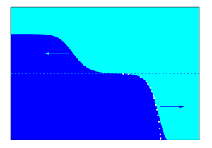
Applying (3.1) and (3.2) to a jump with the upstream interface height  $\eta _{-}=\eta$ propagating into a quiescent fluid ( $\vartheta _{+}=0$), with the interface located at the height $\eta _{+}=\eta _{0}$, as shown in figure 2, after a few rearrangements, we obtain
 $$\begin{gather} \vartheta_{-}^{{\pm}} ={\pm}\frac{(\eta_{0}-\eta)(\eta_{0}+\eta+2\alpha)^{1/2}}{((1-\eta^{2})(\eta_{0}-\eta)+2(\eta+\alpha)(1-\eta_{0}\eta))^{1/2}}, \end{gather}$$
 $$\begin{gather}\dot{\xi}^{{\pm}} ={-}\vartheta_{-}^{{\pm}}\,\frac{1-\eta^{2}}{2(\eta_{0}-\eta)}, \end{gather}$$
where  $\vartheta _{-}^{\pm }$ is the upstream shear velocity, and the plus and minus signs refer to the opposite directions of propagation, i.e. $\dot {\xi }^{+}=-\dot {\xi }^{-}$, which are both permitted by the mass and momentum balance conditions. Because the energy balance (3.3) changes sign with the direction of propagation, in general, only one direction of propagation is permitted for each jump. This does not apply to the jumps that satisfy (3.3) exactly. Such energy-conserving jumps, which can in principle propagate downstream as well as upstream, will be considered in the following.

Figure 2. A jump with the upstream interface height  $\eta _{-}=\eta$ and the shear velocity $\vartheta _{-}=\vartheta$ propagating at speed $\dot {\xi }$ into a still fluid ahead ( $\vartheta _{+}=0$), with the interface located at height $\eta _{+}=\eta _{0}$.
A distinctive feature of these jumps is the invariance of their velocity of propagation (3.5) with  $\alpha$ (Priede Reference Priede2023). It implies that these jumps also conserve circulation. If this is the case, then the $\alpha$ terms in the generalized momentum equation (2.19) cancel out, so making the associated jump condition independent of $\alpha$. For this to happen, the shear velocity (3.4) at $\alpha =0$ has to be the same as that at $\alpha \rightarrow \infty$. This requirement results in $\eta (\eta -\eta _{0})=0$, which has two solutions: $\eta =\eta _{0}$ and $\eta =0$. The first is irrelevant as it corresponds to a uniform state with a constant interface height $\eta _{0}$. The second describes a jump from $\eta _{0}$ to the channel mid-height $\eta =0$. The corresponding upstream shear velocity and the speed of propagation following from (3.4) and (3.5) are $\vartheta _{-}^{\pm }=\pm \eta _{0}$ and $\dot {\xi }^{\pm }=\mp \frac {1}{2}$.
Owing to the symmetry of this jump  $\vartheta _{\pm }=\eta _{\mp }$, the impulse and energy are conserved automatically, i.e. independently of the velocity of propagation. Also, the same symmetry makes both characteristic velocities (2.22) continuous across the jump: ${\unicode{x27E6}} \lambda ^{\pm }{\unicode{x27E7}} =0$. This means that the positive as well as negative characteristics emanating upstream from the jump are parallel to the corresponding characteristics emanating downstream. Likewise, the Riemann invariants (2.21) are also continuous.
The above properties are shared by a broader class of fully conservative jumps that can be sustained by a non-zero downstream shear  $(\vartheta _{+}\not =0)$. The continuity condition ${\unicode{x27E6}} \lambda ^{\pm }{\unicode{x27E7}} =0$, which after a few rearrangements can be rewritten as ${\unicode{x27E6}} (\eta \pm \vartheta )^{2}{\unicode{x27E7}} =0$, yields two pairs of possible solutions:
 $$\begin{gather} (\eta_{+},\vartheta_{+}) ={\pm}(\eta_{-},\vartheta_{-}), \end{gather}$$
 $$\begin{gather}(\eta_{+},\vartheta_{+}) ={\pm}(\vartheta_{-},\eta_{-}). \end{gather}$$
The first solution, corresponding to the plus sign in (3.6), is continuous thus irrelevant. The other three are symmetric jumps that satisfy the energy balance condition (3.3) automatically, as well as that of the impulse (3.2) with  $\alpha =0$. The second solution, corresponding to the minus sign in (3.6), which represents a centrally symmetric jump, conserves the mass and circulation only if $\vartheta _{+}=\pm \eta _{+}$ and $\dot {\xi }=\pm \frac {1}{2}(1-\eta _{+}^{2})$. This is just a particular case of a more general solution that follows from the mass and circulation conservation laws for the second pair of jumps (3.7). In this case, we obtain the speed of propagation, which can be written in terms of the upstream and downstream interface heights as
 \begin{equation} \dot{\xi}^{{\pm}}={\pm}\tfrac{1}{2}(1+\eta_{+}\eta_{-}).\end{equation}
The corresponding shear velocities according to (3.7) are  $(\vartheta _{+},\vartheta _{-})=\mp (\eta _{-},\eta _{+})$. Note that the previous two solutions with $\eta _{+}=0$ and $\eta _{+}=-\eta _{-}$ are particular cases of (3.8).
In marginally hyperbolic shear flows with  $\vartheta _{+}=\vartheta _{-}=\mp 1$, which is a very specific case, fully conservative jumps with discontinuous characteristic velocities are possible. Such jumps propagate at speed $\dot {\xi }^{\pm }=\pm \frac {1}{2}(\eta _{+}+\eta _{-})$, which ensures the conservation of impulse and mass, whilst the energy and circulation are conserved automatically.
In the next section, we show that these fully conservative hydraulic jumps represent a long-wave approximation to the so-called solibores that appear as permanent-shape solutions in the weakly non-hydrostatic approximation described by (2.11) (Esler & Pearce Reference Esler and Pearce2011).
4. Weakly non-hydrostatic analytical solution for solibores
Let us now turn to a weakly non-hydrostatic approximation, which is defined by the dynamical pressure correction (2.14) in the circulation conservation equation (2.12), and search for permanent-shape waves travelling at speed  $c$. Such waves are stationary in the co-moving frame of reference where they vary depending only on $x'=x-ct$. With the time derivative written as $\partial _{t}\equiv -c\partial _{x}$, the last two terms in (2.14) cancel out, and correspondingly (2.12) and (2.13) take the form
 $$\begin{gather} \left(\tfrac{1}{2}\eta(1-\vartheta^{2})-c\vartheta\right)_{x} ={-}\tfrac{1}{3}\left[hD_{t}^{2}h+\tfrac{1}{2}(D_{t}h)^{2}\right]_{x}, \end{gather}$$
 $$\begin{gather}\left(\tfrac{1}{2}\vartheta(1-\eta^{2})-c\eta\right)_{x} = 0, \end{gather}$$
where  $h$ stands for $h^{\pm }=\frac {1}{2}(1\pm \eta )$, and $D_{t}$ stands for $D_{t}^{\pm }\equiv (u^{\pm }-c)\partial _{x}$, with the plus and minus indices referring to the top and bottom layers. Now (4.1) and (4.2) can be integrated once to obtain
 $$\begin{gather} \tfrac{1}{2}\eta(1-\vartheta^{2})-c(\vartheta-\vartheta_{0}) ={-}\tfrac{1}{3}\left[hD_{t}^{2}h+\tfrac{1}{2}(D_{t}h)^{2}\right], \end{gather}$$
 $$\begin{gather}\tfrac{1}{2}\vartheta(1-\eta^{2})-c(\eta-\eta_{0}) = 0, \end{gather}$$
where  $\vartheta _{0}$ and $\eta _{0}$ are the constants of integration. Note that if the fluid far upstream or downstream is at rest ( $\vartheta =0$), then according to (4.4), $\eta _{0}$ is equal to the respective interface height; $c\vartheta _{0}=A$ is the flux of circulation, which is one of the conserved quantities.
Using the identity  $hD_{t}^{\pm }\equiv -h_{0}^{\pm }c\partial _{x}$, which follows from $D_{t}^{\pm }\equiv (u^{\pm }-c)\partial _{x}$ and (4.4) when written in terms of the original variables as $h^{\pm }(u^{\pm }-c)=-h_{0}^{\pm }c$, the right-hand side of (4.3) can be transformed to
 \begin{equation} -\frac{c^{2}}{3}\left[h_{0}^{2}\left((h_{x}/h)_{x}+\frac{1}{2}\,(h_{x}/h)^{2}\right) \right]={-}\frac{c^{2}}{3}\left\{(h_{0}h_{x})^{2}/h\right\} _{x}/{{\eta_{x}}}. \end{equation}
Then multiplying (4.3) with  $\eta _{x}$ and using (4.2) to substitute for $c\eta _{x}$, after a few rearrangements, the resulting equation can be integrated once more to obtain
 \begin{equation} A\eta+B-\frac{1}{4}\,(1-\eta^{2})(1+\vartheta^{2})={-}\frac{c^{2}}{12}\,\frac{1-2\eta_{0} \eta+\eta_{0}^{2}}{1-\eta^{2}}\,{{\eta_{x}}}^{2}, \end{equation}
where  $B$ is a constant of integration that represents another conserved quantity, the flux of impulse. Finally, using (4.4) to eliminate $\vartheta$, we obtain
 \begin{equation} {{\eta_{x}}}^{2}+P(\eta)=0,\end{equation}
where
 \begin{equation} P(\eta)={-}\frac{3}{c^{2}}\,\frac{(1-\eta^{2})(1-\eta^{2}-4(A\eta+B))+4c^{2}(\eta-\eta_{0})^{2}} {1-\eta^{2}+(\eta-\eta_{0})^{2}}\end{equation}
is analogous to potential energy when  ${{\eta _{x}}}^{2}$ is interpreted as kinetic energy with $x$ representing the time. Thus (4.7) can be thought of as describing the conservation of total energy for a body performing periodic oscillations in the potential well defined by (4.8). The oscillations occur between the points at which the velocity-like quantity $\eta _{x}$ changes sign. This happens at the turning points $\eta _{x}=0$, which correspond to two extremes of $\eta$. According to (4.7), these points are the zeros of the numerator of $P(\eta )$. As the latter is a quartic function of $\eta$, in general it can have four roots. For a finite-amplitude solution to be possible, all roots have to be real (Esler & Pearce Reference Esler and Pearce2011). If two roots coincide but the other two are distinct, then the oscillation period becomes infinite, resulting in the so-called solitary wave. If also the other two roots coincide, so that there are two distinct double roots, then we end up with only a half-solitary wave, which is termed the solibore (Esler & Pearce Reference Esler and Pearce2011).
In the following, we focus on the last case and determine the unknown constants in (4.8) by factorizing the numerator of  $P(\eta )$ as
 \begin{equation} (1-\eta^{2})(1-\eta^{2}-4(A\eta+B))+4c^{2}(\eta-\eta_{0})^{2}=(\eta-\eta_{+})^{2}(\eta-\eta_{-})^{2},\end{equation}
where  $\eta _{+}$ and $\eta _{-}$ are two double roots of the quartic defining respectively the downstream and upstream interface heights. Comparing the coefficients at the same powers of $\eta$ on both sides of (4.9), and eliminating $A$ and $B$, we have
 \begin{equation} 4c^{2}(1\pm\eta_{0})^{2}=\left(\eta_{+}+\eta_{-}\pm(1+\eta_{+}\eta_{-})\right)^{2},\end{equation}
which represents a system of two equations corresponding to the same choice of sign on both sides. There are two possible solutions for  $c$ and $\eta _{0}$, depending on the combination of signs when taking the square root of both sides of (4.10). The first solution
 \begin{equation} c={\pm}\frac{1}{2}\,(1+\eta_{+}\eta_{-}),\quad\eta_{0}=\frac{\eta_{+}+\eta_{-}}{1+\eta_{+}\eta_{-}}, \end{equation}
with  $(\vartheta _{+},\vartheta _{-})=\mp (\eta _{-},\eta _{+})$ following from (4.4), corresponds to the conservative jumps with continuous characteristic velocities found in the previous section. The second solution
 \begin{equation} c={\pm}\frac{1}{2}\,(\eta_{+}+\eta_{-}),\quad\eta_{0}=\frac{1+\eta_{+}\eta_{-}}{\eta_{+}+\eta_{-}}, \end{equation}
with  $\vartheta _{+}=\vartheta _{-}=\mp 1$ resulting from (4.4), corresponds to the conservative jumps with discontinuous characteristic velocities. This type of solibore seems to be of little practical relevance because of the very specific shear values required for its existence.
Using the factorization of the numerator of  $P(\eta )$ defined by (4.9), we can integrate (4.7) analytically as
 \begin{align} x(\eta) & =\frac{c}{\sqrt{3}}\int\frac{q(\eta)\,\mathrm{d}\eta}{(\eta-\eta_{+})(\eta-\eta_{-})} \nonumber\\ & =\frac{2c}{\sqrt{3}(\eta_{+}-\eta_{-})}\left[q(\eta_{+})\,\text{arctanh}\left(\frac{q(\eta)}{q(\eta_{+})}\right)-q(\eta_{-})\,\text{arctanh}\left(\frac{q(\eta_{-})}{q(\eta)}\right)\right], \end{align}
where  $q(\eta )=\sqrt {1-\eta ^{2}+(\eta -\eta _{0})^{2}}$, and $\eta _{+}$ and $\eta _{-}$ are ordered so that $q(\eta _{+})\geqslant q(\eta _{-})$. In the symmetric continuous case $\eta _{+}=-\eta _{-}$, when $\eta _{0}=0$ and $c=\pm (1-\eta _{+}^{2})/2$, (4.13) can be written explicitly as $\eta (x)=\eta _{+}\tanh ({2\sqrt {3}x}/({\eta _{+}-\eta _{+}^{-1}}))$.
For a quiescent downstream state, when  $\vartheta _{+}=\eta _{-}=0$, $\eta _{0}=\eta _{+}$ and $c=\pm \frac {1}{2}$, which is practically the most relevant, (4.13) is plotted in figure 3 for various interface heights $\eta _{0}<0$. Note that (4.13) is invariant with the symmetry transformation $\eta \rightarrow -\eta$. Therefore, the solutions with $\eta _{0}>0$ are mirror symmetric images of those with $\eta _{0}<0$ shown in figure 3. It is important to note that the solution for $\eta _{0}=-1$ corresponds to the limit of an infinitesimally shallow bottom layer. As seen, the solibore shape in this limiting case is very similar to that of the gravity current found by Benjamin (Reference Benjamin1968). The difference is mostly at the bottom, which is approached tangentially by the bore, whereas the gravity current approaches it at angle ${\rm \pi} /3$ (von Kármán Reference von Kármán1940). This exact inviscid solution, which contains a singularity at the contact point where the velocity varies as $\sim r^{-1/2}$ with the distance $r$, is outside the scope of the SW approximation.

Figure 3. Solibores advancing into a quiescent downstream state with various interface heights  $\eta _{0}<0$. The dots show the approximate solution of Benjamin (Reference Benjamin1968) for an energy-conserving gravity current.
5. Summary and discussion
In the present paper, we considered a special type of hydraulic jump that, in the two-layer Boussinesq system bounded by a rigid lid, can conserve not only the mass and impulse, as usual, but also the circulation and energy. This is possible only at certain combinations of the upstream and downstream states for which the speed of propagation becomes invariant with the free parameter specifying the contribution of each layer to the interfacial pressure distribution in the generalized SW momentum conservation law.
Jumps propagating into a quiescent fluid are fully conservative only if the interface upstream is located at the mid-height of the channel. The velocity of propagation of such jumps is independent of their height and equal to  $\dot {\xi }=0.5$ in the usual dimensionless units. These fully conservative jumps have a special symmetry, with the upstream shear being equal to the downstream interface height, and vice versa: $\vartheta _{\pm }=\eta _{\mp }$. This symmetry ensures the automatic conservation of the impulse and energy as well as the continuity of both characteristic velocities across the jump. Namely, the positive and negative characteristics emanating on one side of the jump are parallel to the corresponding characteristics emanating on the other side. This apparently allows the jump to propagate without expanding or contracting.
Using this property, we identified a broader class of fully conservative symmetric jumps that propagate in shear flows with velocity  $\dot {\xi }=\pm \frac {1}{2}(1+\eta _{+}\eta _{-})$. The $\pm$ sign here reflects the fact that in the inviscid approximation, theoretically these jumps can propagate in either direction. In real fluids, which are viscous, physical considerations suggest that they have to propagate in the direction that increases the shear. For example, a jump leaving a viscous fluid right behind it at rest would be unphysical.
We also found that if the shear upstream and downstream is marginally hyperbolic, i.e.  $\vartheta _{-}=\vartheta _{+}=\mp 1$, then another type of conservative jump is possible. These jumps are in general asymmetric, have discontinuous characteristic velocities, and propagate at speed $\dot {\xi }=\pm \frac {1}{2}(\eta _{+}+\eta _{-})$. Because of the very specific shear values required for the existence of this type of jump, they appear of little practical relevance.
It is important to note that the fully conservative jumps considered in this study satisfy four conditions but constrain only three out of five jump parameters. Namely, such jumps still have two degrees of freedom – the upstream and downstream interface heights. This is obviously due to the  $\eta \leftrightarrow \vartheta$ symmetry, which is an exclusive feature of the Boussinesq approximation enabling the automatic conservation of two quantities.
Finally, the characteristics of fully conservative jumps were shown to be the same as those of the so-called solibores, which appear as permanent-shape solutions in weakly non-hydrostatic approximation. An exact analytical solution for solibores was obtained.
Note that two such fully conservative jumps feature in the partial lock exchange flow when the lock is taller than the channel mid-height (Politis & Priede Reference Politis and Priede2022). These jumps represent the front of a gravity current, which propagates downstream along the bottom, and a bore, which propagates upstream in the upper half of the channel. Analytical solution (4.13) can be seen in figure 4 to agree well with the two-dimensional DNS results of Khodkar et al. (Reference Khodkar, Nasr-Azadani and Meiburg2017) when the  $x$-axis is scaled by a factor $\sqrt {2}$, which is apparently due to a different internal length scale used in the numerical code for the $x$-coordinate. The necessity of this rescaling becomes obvious when the numerical results of Khodkar et al. (Reference Khodkar, Nasr-Azadani and Meiburg2017) are compared with the inviscid solution of Benjamin (Reference Benjamin1968) for the energy-conserving gravity current. This solution can be used as a benchmark because it is known to provide a good approximation to both experimental and numerical results (Härtel, Meiburg & Necker Reference Härtel, Meiburg and Necker2000). Once the rescaled numerical results match the benchmark solution for the gravity current, they agree also with the solution for solibores obtained in this study. The agreement is very good for both heights of the lock considered. As discussed above, the inviscid solution obtained by Benjamin (Reference Benjamin1968) is very close to the respective solibore solution except in the vicinity of the contact point. It is interesting to note that both cases are equivalent in the SW approximation, but treated somewhat differently in the conventional control volume approach. This, however, does not affect the predicted speed propagation, which is the same for gravity currents (Benjamin Reference Benjamin1968) and internal bores with a vanishingly shallow downstream bottom layer (Klemp et al. Reference Klemp, Rotunno and Skamarock1997).

Figure 4. Comparison of the analytical solution (4.13) with the DNS results of Khodkar et al. (Reference Khodkar, Nasr-Azadani and Meiburg2017) for partial lock exchange flows with lock heights (a)  $h_{-}=0.9$ and (b) $h_{-}=0.8$. The dashed lines show the analytical solution, and the dots show the approximate solution for the energy-conserving gravity current obtained by Benjamin (Reference Benjamin1968). The DNS results shown in the background are from figure 9(e, f) of Khodkar et al. (Reference Khodkar, Nasr-Azadani and Meiburg2017).
The finding that certain large-amplitude hydraulic jumps can be fully conservative while most are not such even in the inviscid approximation, points towards the wave dispersion as a primary mechanism behind the lossy nature of internal bores. Namely, it is the absence of dispersion in solibores that makes the corresponding jumps fully conservative while in general all other jumps are dispersive (Esler & Pearce Reference Esler and Pearce2011). Such dispersive jumps may be amenable to Whitham's modulation theory (Whitham Reference Whitham1965; El & Hoefer Reference El and Hoefer2016) which could resolve the non-uniqueness in their speed of propagation emerging in the hydrostatic SW approximation.
Declaration of interest
The author reports no conflict of interest.


 Open access