2. Orientation of axisymmetric grains

The ability of axisymmetric grains to orient and align introduces an additional degree of complexity to their mechanical response. Experimental and numerical measurements suggest that the orientation and alignment of these grains react to the flow and the boundary conditions. A convenient representation of the grains’ orientation can be constructed by taking the second moment of the orientation distribution

(2.1)\begin{equation} \boldsymbol{\mathsf{A}} = \oint_{s^2} f(\boldsymbol{k}) \boldsymbol{k} \otimes \boldsymbol{k} \,{\rm d}a , \end{equation}

where $\pm \boldsymbol {k}$ is the orientation, $f(\boldsymbol {k})\geq 0$ is the probability density function, $s^2$ denotes the unit sphere and $\oint _{s^2} f(\boldsymbol {k})\,{\rm d}a=1$. It follows from (2.1) that the orientational tensor $\boldsymbol{\mathsf{A}}$ is a second-order symmetric positive semi-definite tensor with a unit trace. It was proposed in Nadler et al. (Reference Nadler, Guillard and Einav2018) that the tendency of axisymmetric grains to align, when subjected to flow, can be well described by the evolution equation of the orientational tensor

(2.2)\begin{equation} \dot{\boldsymbol{\mathsf{A}}} = \boldsymbol{\mathsf{W}}\boldsymbol{\mathsf{A}} - \boldsymbol{\mathsf{A}}\boldsymbol{\mathsf{W}} + \lambda \left[\boldsymbol{\mathsf{A}}\boldsymbol{\mathsf{D}} + \boldsymbol{\mathsf{D}}\boldsymbol{\mathsf{A}} - 2\left[\boldsymbol{\mathsf{D}} \boldsymbol{\cdot} \boldsymbol{\mathsf{A}} \right]\boldsymbol{\mathsf{A}} \right] - \psi D' [\boldsymbol{\mathsf{A}} - \boldsymbol{\mathsf{I}}/3], \end{equation}

where $\dot {\boldsymbol{\mathsf{A}}}$ is the material time derivative of the orientational tensor, $\boldsymbol{\mathsf{W}}$ is the vorticity tensor, $\boldsymbol{\mathsf{D}}$ is the rate of deformation, $\boldsymbol{\mathsf{I}}$ is the identity tensor, $\boldsymbol{\mathsf{A}} \boldsymbol {\cdot } \boldsymbol{\mathsf{D}}=\operatorname {tr} (\boldsymbol{\mathsf{A}} \boldsymbol{\mathsf{D}}^T)$ is the tensor scalar product, $\lambda$ and $\psi$ are constitutive model parameters and $D'= \sqrt {\boldsymbol{\mathsf{D}}' \boldsymbol {\cdot } \boldsymbol{\mathsf{D}}'}$ is the magnitude of the deviatoric part of the rate of deformation. Here we assume that the rate of collisions that drives the gains toward disorder is proportional to the magnitude of the deviatoric part of the rate of deformation. The phenomenological model parameters were determined by numerical simulations of simple shear flows using DEM (Nadler et al. Reference Nadler, Guillard and Einav2018). It was assumed that the model parameters are only functions of the grain shape $r_g=(l-d)/(l+d)$, where $l$ and $d$ are the grain's geometrical length and diameter, respectively, and take the forms

(2.3a,b)\begin{equation} \lambda(r_g)=(2/{\rm \pi})\tan^{{-}1}\left(5.5 \, r_g\right) , \quad \psi(r_g)=0.85 \exp({-}4 \,r_g^2). \end{equation}

As simple shear flow is primarily homogeneous, the role of orientational field could not be studied using these simulations and was not included in (2.2). In general, flow is not homogenous and, hence, orientational diffusion can play a significant role.

2.1. Orientational diffusion

The evolution law (2.2) was shown to perform well for homogeneous orientation and rate of deformation $(\operatorname {grad} \boldsymbol{\mathsf{A}} = \boldsymbol {0},\, \operatorname {grad} \boldsymbol{\mathsf{D}} = \boldsymbol {0})$. In this case, the interaction through collisions and contacts with the surroundings was neglected. However, there are evidences that orientational diffusion is important (Guillard et al. Reference Guillard, Marks and Einav2017; Hidalgo et al. Reference Hidalgo, Szabó, Gillearot, Börzsönyi and Weinhart2018). This is supported by Hidalgo et al. (Reference Hidalgo, Szabó, Gillearot, Börzsönyi and Weinhart2018) where flows down an incline were investigated and an inhomogeneous orientational field through the height was measured. We relate the inhomogeneous orientation field through the height of the flow to orientational diffusion. To include such orientational diffusion, the evolution equation (2.2) is generalized by adding a diffusion contribution. Recall that a general balance law has the form

(2.4)\begin{equation} \dot{\boldsymbol{\mathsf{A}}} = \boldsymbol{\mathsf{P}} + \operatorname{div} \boldsymbol{\mathsf{G}} , \end{equation}

where $\boldsymbol{\mathsf{P}}$ is a source term and $\boldsymbol{\mathsf{G}}$ is a non-convective flux term. In general, the source term includes supply and production, however, on physical ground, we eliminate the supply term and consider the source term to be only due to production. By comparison of (2.4) and (2.2), the right-hand side of (2.2) includes only the production term $\boldsymbol{\mathsf{P}}$ whereas the diffusion term $\operatorname {div} \boldsymbol{\mathsf{G}}$ is not included. Analogous to Fick's law for diffusion, we propose the non-convective flux $\boldsymbol{\mathsf{G}}$ to be proportional to the spatial gradient of the orientational tensor and the magnitude of the deviatoric part of the rate of deformation in the form

(2.5)\begin{equation} \boldsymbol{\mathsf{G}} = \alpha D' \operatorname{grad} \boldsymbol{\mathsf{A}}, \end{equation}

where $\alpha$ is an orientational diffusion coefficient that has the dimensions of length squared. As diffusion occurs due to collisions, the diffusion flux is taken to be proportional to the deviatoric part of the rate of deformation. The generalized evolution law takes the form

(2.6)\begin{align} \dot{\boldsymbol{\mathsf{A}}} = \boldsymbol{\mathsf{W}}\boldsymbol{\mathsf{A}} - \boldsymbol{\mathsf{A}}\boldsymbol{\mathsf{W}} + \lambda \left[ \boldsymbol{\mathsf{A}}\boldsymbol{\mathsf{D}} + \boldsymbol{\mathsf{D}}\boldsymbol{\mathsf{A}} - 2 \right[ \boldsymbol{\mathsf{A}} \boldsymbol{\cdot} \boldsymbol{\mathsf{D}} \left] \boldsymbol{\mathsf{A}} \right] - \psi D' \left[ \boldsymbol{\mathsf{A}} - \boldsymbol{\mathsf{I}}/3 \right] + \operatorname{div} \left[ \alpha D' \operatorname{grad} \boldsymbol{\mathsf{A}} \right] . \end{align}

This generalized evolution law (2.6) must satisfy two requirements that are studied in the following section.

2.2. Admissibility of the modified evolution law

The generalized evolution law is admissible if it guarantees that $\boldsymbol{\mathsf{A}}$ is positive semi-definite and it has a unit trace, $\operatorname {tr}\boldsymbol{\mathsf{A}}=1$, for all processes. Utilizing the spectral representation of $\boldsymbol{\mathsf{A}}$, these requirements can be verified by analyzing the evolution of the eigenvalues. The spectral representation of the symmetric orientational tensor $\boldsymbol{\mathsf{A}}$ has the form

(2.7)\begin{equation} \boldsymbol{\mathsf{A}}= \sum_{i=1} ^{3} a_i \, \boldsymbol{a}_i \otimes \boldsymbol{a}_i , \end{equation}

where $a_i$ are the eigenvalues and $\boldsymbol {a}_i$ are the associated orthonormal eigenvectors. The Eigenvalues of the orientational tensor $\boldsymbol{\mathsf{A}}$ represent the portion of grains in the direction of the associated eigenvectors. The two requirements are satisfied if and only if all eigenvalues are non-negative, $a_i \geq 0$, and the summation of eigenvalues equals one, $a_1+a_2+a_3 =1$. In the following sections, we prove that for all initial conditions that satisfy these two requirements, the generalized evolution law (2.6) guarantees that $\operatorname {tr}{\boldsymbol{\mathsf{A}}}=1$ and all eigenvalues remain non-negative, for all processes. To show these, we utilize Cartesian coordinates $\{x_i\}$ and use the standard convenient notation $\square,_i = \partial \square / \partial x_i$ for partial derivatives. In the following derivations the summation convention does not apply. First, it is necessary to show that $\operatorname {tr} \boldsymbol{\mathsf{A}} = 1$, which can be achieved by verifying that the evolution law (2.6) satisfies $\operatorname {tr} \dot {\boldsymbol{\mathsf{A}}} = 0$ for all processes.

Proposition 2.1 The evolution law satisfies $\operatorname {tr} \dot {\boldsymbol{\mathsf{A}}} =0$ for all processes.

Proof. It was already shown in Nadler et al. (Reference Nadler, Guillard and Einav2018) that the production term is traceless, that is

(2.8)\begin{equation} \operatorname{tr} \left[ \boldsymbol{\mathsf{W}}\boldsymbol{\mathsf{A}} - \boldsymbol{\mathsf{A}}\boldsymbol{\mathsf{W}} + \lambda \left( \boldsymbol{\mathsf{A}}\boldsymbol{\mathsf{D}} + \boldsymbol{\mathsf{D}}\boldsymbol{\mathsf{A}} - 2 \left( \boldsymbol{\mathsf{D}} \boldsymbol{\cdot} \boldsymbol{\mathsf{A}} \right)\boldsymbol{\mathsf{A}} \right) - \psi D^\prime \left( \boldsymbol{\mathsf{A}} - \boldsymbol{\mathsf{I}}/3 \right) \right]= 0. \end{equation}

Hence, it is only necessary to show that the diffusion term is traceless

(2.9)\begin{equation} \operatorname{tr} \left[\operatorname{div}\left[ D^\prime \alpha \, \operatorname{grad} \left( \boldsymbol{\mathsf{A}} \right) \right]\right] = 0, \end{equation}

which can be expressed as

(2.10)\begin{equation} \sum_{j=1}^{3} \left[ (\alpha D^\prime),_j \left(\sum_{i=1}^{3} a_i,_j\right) + \alpha D^\prime \left(\sum_{i=1}^{3} a_i,_{jj}\right) \right] =0, \end{equation}

where the detailed derivations are provided in the Appendix A. Recall that $\sum _{i=1} ^{3} a_i =1$, hence by taking the spatial derivatives, the following identities hold

(2.11a,b)\begin{equation} \sum_{i=1} ^{3} a_{i_{,j}}= 0, \quad\sum_{i=1} ^{3} a_{i_{,jj}}=0. \end{equation}

Substitutions of these identities into (2.10) yields

(2.12)\begin{equation} \operatorname{tr} \left [ \operatorname{div} \left[ \alpha D^\prime \, \operatorname{grad} \left( \boldsymbol{\mathsf{A}} \right) \right] \right ] = 0, \end{equation}

which shows the desirable property

(2.13)\begin{equation} \operatorname{tr} \dot {\boldsymbol{\mathsf{A}}} = 0, \end{equation}

for all processes.

To show that the evolution law (2.6) does not yield negative eigenvalues, we consider the case when an eigenvalue vanishes. In this case, if the rate of evolution of that eigenvalue is non-negative, it cannot become negative. Given an admissible state, that is, all eigenvalues are non-negative, when an eigenvalue vanishes, $a_i=0$, this is either a local minimum or it vanishes at some neighbourhood. For both cases we have the properties

(2.14a–c)\begin{equation} a_i=0, \quad a_{i,_{j}} = 0 , \quad a_{i,_{jj}}\geq0 , \end{equation}

for all $j$. It should be noted that (2.14a–c) are necessary conditions but not sufficient for a minimum. Next, it is necessary to show that if an eigenvalue vanishes, $a_i = 0$, the evolution law (2.6) guarantees that $\dot {a}_i \geq 0$ for all processes.

Proposition 2.2 The evolution law guarantees that all eigenvalues are non-negative for all processes.

Proof. Consider the evolution of the orientational tensor defined in (2.2) and the spectral representation (2.7) where the eigenvectors form orthonormal basis such that $\boldsymbol {a}_i \boldsymbol {\cdot } \boldsymbol {a}_j = \delta _{ij}$. The material time derivative of the orientational tensor is

(2.15)\begin{equation} \dot{\boldsymbol{\mathsf{A}}}= \sum_{i=1} ^{3} \dot{a_i} \, \boldsymbol{a}_i \otimes \boldsymbol{a}_i + \sum_{i=1} ^{3} a_i \, \dot{\overline{\boldsymbol{a}_i \otimes \boldsymbol{a}_i}}. \end{equation}

Orthonormality of the eigenvectors can be expressed as $\dot {\boldsymbol {a}}_i \boldsymbol {\cdot } \boldsymbol {a}_i = 0$ and $\boldsymbol {a}_{i,_{j}} \boldsymbol {\cdot } \boldsymbol {a}_i = 0$. Taking the scalar product of (2.15) with $\boldsymbol {a}_i \otimes \boldsymbol {a}_i$ yields expression for the time derivative of the eigenvalues as

(2.16)\begin{equation} \dot{a}_i = \dot{\boldsymbol{\mathsf{A}}} \boldsymbol{\cdot} \boldsymbol{a}_i \otimes \boldsymbol{a}_i. \end{equation}

Substitution of (2.6) and (2.14a–c) into (2.16) yields the instantaneous evolution law of the vanishing eigenvalue as

(2.17)\begin{equation} \dot{a_i} = \frac{1}{3}\psi D^\prime + \alpha D^\prime \sum_{j=1}^3 \left[ a_{i,_{jj}} + 2 \sum_{k=1}^3 a_k \left( \boldsymbol{a}_{k,_{j}} \boldsymbol{\cdot} \boldsymbol{a}_i \right)^2 \right] , \end{equation}

where more details of the derivation are included in Appendix A. As $D^\prime >0$, $\psi >0$ and the term in the brackets is non-negative, then taking $\alpha >0$ guarantees that $\dot {a}_i>0$ when $a_i=0$. This shows that given $\alpha >0$, all the eigenvalues are non-negative for all processes. More specifically, because $\sum _{i=1} ^{3} a_i =1$ and $a_i \geq 0$, then all the eigenvalues are bounded, i.e. $0 \leq a_i \leq 1$, as required. In general, the coefficient $\alpha$ can be function of all the invariants of $\boldsymbol{\mathsf{D}}$, $\boldsymbol{\mathsf{A}}$ and $\operatorname {grad} \boldsymbol{\mathsf{A}}$ as well as the pressure, $p$, and the aspect ratio, $r_g$, and other properties of the grains.

2.3. Initial and boundary conditions

The evolution law in (2.6) is an initial boundary-valued problem, giving a first-order differential equation in time and a second-order differential equation in space. Therefore, proper initial and boundary conditions for $\boldsymbol{\mathsf{A}}$ are required. The initial value of $\boldsymbol{\mathsf{A}}$ in the domain must be specified as the initial conditions. In addition, the boundary conditions must be specified and can significantly change the orientational field and the associate flow. The boundary condition can be Dirichlet (imposing the value of $\boldsymbol{\mathsf{A}}$), Neumann (imposing the value of the spatial derivative of $\boldsymbol{\mathsf{A}}$) or mixed type. The interaction of the grains with the boundary is governed by the surface properties, grain orientation and the flow. Such interactions drive the grains to align with the boundary surface by providing orientational flux. Motivated by the orientational flux term proposed in (2.5) and the commonly used jump boundary condition, we introduce an orientational jump boundary condition, where we assert that the jump is proportional to the rate of collisions, that is, the deviatoric part of the rate of deformation, $D'$, and the gradient of $\boldsymbol{\mathsf{A}}$ in the normal direction to the boundary

(2.18)\begin{equation} [\kern-1pt[ \boldsymbol{\mathsf{A}} ]\kern-1pt] ={-}\nu \, D'\, \frac{\partial \boldsymbol{\mathsf{A}}}{\partial n}, \end{equation}

where $[\kern-1pt[ \boldsymbol{\mathsf{A}} ]\kern-1pt] =\boldsymbol{\mathsf{A}}^+ - \boldsymbol{\mathsf{A}}_s$ is the jump, $\boldsymbol{\mathsf{A}}^+$ is the orientation of grains in contact with the boundary, $\boldsymbol{\mathsf{A}}_s$ is the orientation of boundary surface, $n$ is the normal direction to the boundary and $\nu$ is a scalar with dimensions of time $\times$ length that characterizes the properties of the boundary interaction with the grains in contact. This jump boundary condition suggests that the orientational flux is proportional to the orientation jump, that is, the orientation of the grains in direct contact with the boundary depends on the flow and the properties of the boundary. The limit cases can be identified where $\nu \rightarrow 0$, yields no jump on the boundary, that is, the orientation of the grains in contact with the boundary is completely aligned with the boundary and $\nu \rightarrow \infty$, yields $\partial \boldsymbol{\mathsf{A}} / \partial n=0$, that is, the orientational flux from the boundary vanishes. On physical ground, $\nu \geq 0$ such that the orientational flux is in the same direction as the jump. In general, the coefficient $\nu$ can be a function of all the invariants of $\boldsymbol{\mathsf{D}}$, $\boldsymbol{\mathsf{A}}$ and $\partial \boldsymbol{\mathsf{A}} /\partial n$ as well as the pressure, $p$ and the properties of the grains and the boundary surface.

The orientation evolution law (2.6) and the jump boundary conditions (2.18) complete the governing equations of the orientational tensor, given the vorticity, $\boldsymbol{\mathsf{W}}$ and the rate of deformation $\boldsymbol{\mathsf{D}}$. Next, to close the set of governing equations, conservation of mass and the balance of linear momentum supplemented by a constitutive law are introduced, where the constitutive law is an explicit function of the orientational tensor and couples the response of the system.

3. Anisotropic $\mu (I)$ rheology of axisymmetric grains

The conservation of mass and balance of linear momentum are respectively used to solve for the density $\rho$ and the velocity $\boldsymbol {v}$ fields

(3.1a,b)\begin{equation} \dot{\rho}+\rho \operatorname{div} \boldsymbol{v} = 0, \quad \rho \dot{\boldsymbol{v}} = \rho\boldsymbol{b} + \operatorname{div} \boldsymbol{\sigma}, \end{equation}

where $\boldsymbol {b}$ is the body force and $\boldsymbol {\sigma }$ is the Cauchy stress. The rheological response of granular media is described by a constitutive law for the stress $\boldsymbol {\sigma }$ developed in flowing grains. Physically, the rheological response is a macro-scale manifestation of the characteristic of the contacts and collisions between grains in the microstructure. The characteristic of the contacts and collisions strongly depends on the grains shape, roughness, orientation and flow which was investigated in Börzsönyi et al. (Reference Börzsönyi, Szabó, Törös, Wegner, Török, Somfai, Bien and Stannarius2012); Börzsonyi et al. (Reference Börzsönyi, Somfai, Szabó, Wegner, Mier, Rose and Stannarius2016), Guillard et al. (Reference Guillard, Marks and Einav2017) and Nagy et al. (Reference Nagy, Claudin, Börzsönyi and Somfai2017). It was observed (Nagy et al. Reference Nagy, Claudin, Börzsönyi and Somfai2017) that for simple shear flows, the required shear traction to maintain the flow, dramatically decreases as the grains become more aspherical. This response is contributed to the ability of axisymmetric grains to align with respect to the flow (Nadler Reference Nadler2021), which, in turn, yields a decrease in the resistance of grains to slip with respect to each other. Here, we adopted the simple form of anisotropic inertia rheology for incompressible flow, proposed in Nadler (Reference Nadler2021) as

(3.2)\begin{align} \boldsymbol{\sigma} = \tilde{\boldsymbol{\sigma}}(I,p,\boldsymbol{\mathsf{D}},\boldsymbol{\mathsf{A}};r_g) ={-}p \boldsymbol{\mathsf{I}} + p\mu(I) \phi(r_g) \left[ \bar{\boldsymbol{\mathsf{D}}} + \eta(r_g) \left[ \boldsymbol{\mathsf{A}}\bar{\boldsymbol{\mathsf{D}}} + \bar{\boldsymbol{\mathsf{D}}}\boldsymbol{\mathsf{A}} - 2/3 \left( \bar{\boldsymbol{\mathsf{D}}} \boldsymbol{\cdot} \boldsymbol{\mathsf{A}} \right) \boldsymbol{\mathsf{I}} \right] \right], \end{align}

where $\bar {\boldsymbol{\mathsf{D}}}=\boldsymbol{\mathsf{D}}/D$ is the direction of the rate of deformation and $\mu (I)$ is the friction. The construction of (3.2) is a generalization of the isotropic inertia rheology (Jop, Forterre & Pouliquen Reference Jop, Forterre and Pouliquen2006) which depends on the dimensionless inertia number $I = D d /\sqrt {p/\rho _s}$, where $D= \sqrt {\boldsymbol{\mathsf{D}} \boldsymbol {\cdot } \boldsymbol{\mathsf{D}}}$, $d$, $p$ and $\rho _s$ are the magnitude of the rate of deformation, grain diameter, pressure and the solid density, respectively. The phenomenological inertia rheology relation is $\mu (I)=\mu _s+ \mu _1 I^\beta$, where $\mu _s$, $\mu _1$ and $\beta$ are model parameters. The parameters $\phi$ and $\eta$ are assumed to be only functions of the aspect ratio, $r_g$. The proposed inertia rheology is valid for incompressible flow, hence the conservation of mass is satisfied and the pressure is a Lagrange multiplier. For further discussion of the form (3.2) see Nadler (Reference Nadler2021). The associate initial and boundary conditions of the velocity and stress fields are required for the solution of the conservation of mass and the balance of linear momentum. Two types of boundary conditions are considered which should be decomposed to the normal direction, $\boldsymbol {n}$, and the tangential direction to the boundary. In the normal direction, the boundary conditions have the form

(3.3)\begin{equation} [\kern-1pt[ \rho\boldsymbol{v} ]\kern-1pt] \boldsymbol{\cdot} \boldsymbol{n} = 0 \quad \text{or} \quad \boldsymbol{\sigma} \boldsymbol{n} \boldsymbol{\cdot} \boldsymbol{n} ={-}p_b, \end{equation}

which are the mass flux or the traction boundary conditions, respectively, and $p_b$ is the prescribed pressure. In the tangential directions, the boundary conditions have the form

(3.4)\begin{equation} \mathbb{P} [\kern-1pt[ \boldsymbol{v} ]\kern-1pt] ={-}\mathbb{P}\nu_t \boldsymbol{\sigma} \boldsymbol{n} \quad \text{or} \quad \mathbb{P}\boldsymbol{\sigma} \boldsymbol{n} = \boldsymbol{\tau}_b, \end{equation}

where $\mathbb {P} = \boldsymbol{\mathsf{I}} - \boldsymbol {n} \otimes \boldsymbol {n}$ is the projection, $[\kern-1pt[ \boldsymbol {v} ]\kern-1pt]$ is the velocity jump, $\nu _t$ is a model parameter characterizing the interaction between the boundary surface and the flow and $\boldsymbol {\tau }_b$ is the prescribed tangential traction. The special case of the no-slip condition is $\nu _t=0$, however, in general, the coefficient $\nu _t$ can be a function of the invariants of $\boldsymbol {v}$ and $\boldsymbol {\sigma }$ as well as the properties of the grains and the boundary surface.

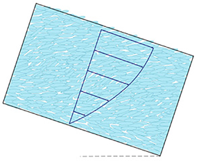
4. Flow down an incline

The evolution law (2.6) can capture inhomogeneous orientational field for general flow, and can accommodate orientational boundary conditions. The standard experiment to study granular flows is a simple shear flow, however, such flow is primarily homogeneous which is too simple for our interest. Granular flow down an incline, depicted in figure 1, is relatively a simple flow that exhibits inhomogeneous fields. Flow down an incline was investigated experimentally and numerically in Hidalgo et al. (Reference Hidalgo, Szabó, Gillearot, Börzsönyi and Weinhart2018), where the orientational field was measured. We use the observations in Hidalgo et al. (Reference Hidalgo, Szabó, Gillearot, Börzsönyi and Weinhart2018) to examine the performance of the proposed model. However, the data provided in Hidalgo et al. (Reference Hidalgo, Szabó, Gillearot, Börzsönyi and Weinhart2018) does not include the orientation near the surface and, hence, cannot be compared with the prediction of the proposed model to understand the diffusion response and the orientational boundary conditions. For a steady flow, the inclination angle is bounded by a small angle below which no flow occurs, and a large angle above which no steady flow is possible because gravity overcomes the friction and acceleration persists. We investigate only an inclination angle where a steady-state flow exists. For our analysis, we consider a steady-state flow where the orientation, velocity and pressure are only functions of the height and are independent of time

(4.1a–c)\begin{equation} p = p(y), \quad \boldsymbol{v} = v(y) \boldsymbol{i}, \quad \boldsymbol{\mathsf{A}} = \boldsymbol{\mathsf{A}}(y). \end{equation}

It follows that at steady state

(4.2a,b)\begin{equation} \dot{\boldsymbol{v}} = \frac{\partial \boldsymbol{v}}{\partial t}+ \left(\operatorname{grad} \boldsymbol{v} \right) \boldsymbol{v} = \boldsymbol{0}, \quad \dot{\boldsymbol{\mathsf{A}}} = \frac{\partial \boldsymbol{\mathsf{A}}}{\partial t} + \left(\operatorname{grad} \boldsymbol{\mathsf{A}}\right) \boldsymbol{v} = \boldsymbol{0}, \end{equation}

and the governing equations are

(4.3a,b)\begin{equation} \dot{\boldsymbol{\mathsf{A}}}=\boldsymbol{0}, \quad \rho \boldsymbol{b} + \operatorname{div} \boldsymbol{\sigma} = \boldsymbol{0}, \end{equation}

where $\dot {\boldsymbol{\mathsf{A}}}$ is defined in (2.6), the body force is $\boldsymbol {b}= g (\sin \theta \, \boldsymbol {i} + \cos \theta \, \boldsymbol {j} )$ and $\boldsymbol {\sigma }$ has the form in (3.2). By (4.1a–c) and using the notation $v'={\rm d}v/{{\rm d}y}$, the vorticity and the rate of deformation take the forms

(4.4a,b)\begin{equation} \boldsymbol{\mathsf{W}}=\frac{v'}{2} \left( \boldsymbol{i} \otimes \boldsymbol{j} - \boldsymbol{j} \otimes \boldsymbol{i}\right), \quad \boldsymbol{\mathsf{D}}=\frac{v'}{2} \left( \boldsymbol{i} \otimes \boldsymbol{j} + \boldsymbol{j} \otimes \boldsymbol{i} \right) . \end{equation}

The boundary conditions (2.18), (3.3) and (3.4) are specified at the boundaries as

(4.5)\begin{gather} [\kern-1pt[ \boldsymbol{\mathsf{A}} ]\kern-1pt] = \nu \, D'\, \frac{{\rm d} \boldsymbol{\mathsf{A}}}{{\rm d} y}, \quad v = \nu_t \boldsymbol{\sigma} \boldsymbol{j} \boldsymbol{\cdot} \boldsymbol{i} , \quad \text{at} \ y=0 , \end{gather}

(4.6)\begin{gather} \frac{{\rm d} \boldsymbol{\mathsf{A}}}{{\rm d} y}=\boldsymbol{0} , \quad \boldsymbol{\sigma} \boldsymbol{j} = \boldsymbol{0} ,\quad \text{at} \ y=h , \end{gather}

where (4.6)$_1$ imposes no orientational flux, and the free surface boundary condition is (4.6)$_2$. These provide a complete set of equations to solve for the unknown fields (4.1a–c). As this system of ordinary differential equations (ODEs) is nonlinear, numerical solutions are obtained using standard finite differences method. Convergence of the solution is verified by a sequence of grid refinements.

Figure 1. Schematic of flow of axisymmetric grains down an incline of angle $\gamma$.

Here we are interested in studying the influence of the coefficients $\alpha$ and $\nu$ in the proposed generalized orientational model on the orientation, velocity and pressure fields. Due to the lack of data, we do not attempt to relate the model coefficients directly to the grain's properties and the flow, but rather consider them as constants and investigate their influence on the model predictions. It should be noted that when $\alpha$ is taken to be a constant, then (2.6) becomes rate independent. Similar to Hidalgo et al. (Reference Hidalgo, Szabó, Gillearot, Börzsönyi and Weinhart2018), we consider the flow of cylindrical glass rods of diameter $d = 1.9\,{\rm mm}$ and length $l = 3.5\,d$ down an incline. The height of the steady state flow is set large enough compared to the size of grains, i.e. ${H}/{d}\approx 10^2$, such that a continuum model is valid. It follows that the aspect ratio is $r_g=0.55$ and the value of the model parameters, $\lambda =0.8$ and $\psi =0.25$, are taken from Nadler et al. (Reference Nadler, Guillard and Einav2018). Although the evolution law of the orientation (2.6) is rate independent, the orientational boundary condition (2.18) is rate dependent for non-vanishing $\nu$, hence, for $\nu >0$, there is a coupling between the velocity and the orientational fields. In the following simulations, the values of the model parameters are

(4.7a–h)$$\begin{gather} \phi=1 ,\quad \eta={-}0.9,\quad \rho_s=2500 \,{\text{kg}}\,{\text{m}^{{-}3}} ,\quad \mu_s=10^{{-}1} ,\quad \mu_1=10^{2} ,\quad \beta=1 ,\nonumber\\ \rho=0.1\, {\text{kg}}\,{\text{m}^{{-}3}} ,\quad \gamma = 30^{{\circ}}, \end{gather}$$

where the values of $\phi$ and $\eta$ are taken from Nadler (Reference Nadler2021), and for simplicity we adopt the no-slip condition, $\nu _t=0$, for the velocity jump at the contact boundary. The properties of the particular grains including, shape (ellipsoidal, true cylinder), aspect ratio and internal friction are represented by the six model parameters.

To represent the orientational field, we define the preferred orientation as the angle of the largest eigenvalue with respect to the incline direction, calculated by

(4.8)\begin{equation} \theta = \tan^{{-}1}\frac{\boldsymbol{a}_3 \boldsymbol{\cdot} \boldsymbol{j} }{\boldsymbol{a}_3 \boldsymbol{\cdot} \boldsymbol{i} }, \end{equation}

where $0 \leqslant a_1 \leqslant a_2 \leqslant a_3 \leqslant 1$ are the sorted eigenvalues of $\boldsymbol{\mathsf{A}}$, and $\{\boldsymbol {a}_1,\boldsymbol {a}_2,\boldsymbol {a}_3 \}$ are the associated eigenvectors. For the measure of alignment, we consider the nematic order (Nagy et al. Reference Nagy, Claudin, Börzsönyi and Somfai2017) defined as the largest eigenvalue $1/3\leq a_3\leq 1$. Additional useful alignment measure is the ordering (Nadler et al. Reference Nadler, Guillard and Einav2018; Nadler Reference Nadler2021) defined as

(4.9)\begin{equation} \zeta = \sqrt{\tfrac{1}{2} \left((a_1-a_2)^2 + (a_1-a_3)^2 + (a_2-a_3)^2 \right)}, \end{equation}

where $0 \leqslant \zeta \leqslant 1$, such that, $\zeta =0$ represents no alignment $(a_1=a_2=a_3=1/3)$ and $\zeta =1$ represents a full alignment $(a_1=a_2=0,a_3=1)$.

The following results are normalized with respect to the flow height

(4.10a–d)\begin{equation} \bar{y}=\frac{y}{h} , \quad \bar{v}=\frac{v}{h} , \quad \bar{\alpha}=\frac{\alpha}{h^2} , \quad \bar{\nu}=\frac{\nu}{h} , \end{equation}

and the inclined plane is considered to be perfectly flat in the $xz$ plane, hence its orientation is described by

(4.11)\begin{equation} \boldsymbol{\mathsf{A}}_s = \tfrac{1}{2} \left( \boldsymbol{i} \otimes \boldsymbol{i} + \boldsymbol{k} \otimes \boldsymbol{k} \right). \end{equation}

The boundary orientation, $\boldsymbol{\mathsf{A}}_s$, represents the topology and orientation of the boundary surface, that is, for irregular boundary surface the boundary orientation should take a more isotropic form $\boldsymbol{\mathsf{A}}_s\rightarrow \boldsymbol{\mathsf{I}}/3$.

Figures 2 and 3 show the influence of the diffusion coefficient, $\bar {\alpha }$, and the jump coefficient, $\bar {\nu }$, on the orientational field represented by the preferred orientation $\theta$, the nematic order, $a_3$, and the ordering $\zeta$. These figures show results for $\bar {\alpha }=\{0.001,0.005,0.01\}$ and $\bar {\nu }=\{0,0.02,0.05\}$. Figure 2 depicts the influence of the diffusion coefficient and figure 3 depicts the influence of the orientational boundary jump. Larger values of the diffusion coefficient are not presented because the orientation does not reach an equilibrium state, and larger values of the orientational boundary jump are not presented because they eliminate the influence of the boundary. Figures 2(a,d) and 3(a,d) show, as expected, that a larger diffusion coefficient enhances the influence of the boundary, where the equilibrium orientation is obtained further away from the boundary. It is very interesting to note that the orientational angle $\theta$ shows a non-monotonic response, where the angle increases as the grains located at some distance from the boundary reach a maximum value and then decreases to the equilibrium angle far enough from the boundary as depicted in figure 2(a,d). This non-monotonic field, predicted by the model, is consistent with the orientational angle observed in Hidalgo et al. (Reference Hidalgo, Szabó, Gillearot, Börzsönyi and Weinhart2018). This non-monotonic field is due to the orientational flux from the boundary and, hence, reduces with a larger orientational boundary jump as depicted in figure 3(a,d). In these figures, for $\bar {\nu }=0$ (no orientational boundary jump), the grains in contact with the boundary plane are completely aligned with the plane, but for larger $\bar {\nu }$, the orientation of grains in contact with the boundary plane approaches the equilibrium orientation yielding a more homogenous orientational field. It is observed that the diffusion coefficient controls the location of the maximum angle, and the orientational boundary jump coefficient controls the magnitude of the maximum angle. Figures 2(b,e) and 3(b,e) show that the nematic order measured by the largest eigenvalue is minimum at the boundary and converges to the equilibrium away from the boundary, where the diffusion coefficient controls the rate of convergence. The equilibrium state is associated with vanishing orientational flux; hence, the orientation of the grains is governed only by the production term in (2.6) as was studied in Nadler et al. (Reference Nadler, Guillard and Einav2018) for homogeneous fields. As the orientational flux from the boundary reduces, for increasing values of $\bar {\nu }$, the nematic order becomes more homogeneous. Figures 2(c, f) and 3(c, f) show a non-monotonic field of the ordering $\zeta$, which accounts for the overall alignment. For $\nu =0$, the grains in contact with the boundary are forced by the no-jump orientational boundary condition to be in a state of isotropic distribution in the $xz$ plane (transverse isotropy). As grains that are oriented in the $\boldsymbol {k} \otimes \boldsymbol {k}$ direction near the boundary rotate toward the equilibrium state away from the boundary, the overall ordering shows a non-monotonic field with the minimum near the boundary where the diffusion coefficient governs the distance from the boundary. This non-monotonic response diminishes, as depicted in figures 2(c, f) and 3(c, f), for larger values of the boundary orientational jump $\bar {\nu }$ associated with decrease of the boundary flux the equilibrium state is obtained closer to the boundary. In addition, figures 2 and 3 demonstrate that the jump boundary condition (2.18) yields flow-dependent orientation of the grains in direct contact with the boundary. As can be observed in figures 2 and 3, the size of the boundary layer increases with the orientation diffusion coefficient as the boundary flux diffuses further into the bulk. Here we limit the values of the orientational diffusion, $\bar {\alpha }$, such that the equilibrium orientation is obtain within the domain. However, for larger values of the orientation diffusion the equilibrium orientation is not obtained within the domain.

Figure 2. The influence of the diffusion coefficient, $\bar {\alpha }$, on the orientational angle, nematic order and ordering fields for $\bar {\nu }=0$ and $\bar {\nu }=0.05$: (a) $\bar {\nu }=0$, (b) $\bar {\nu }=0$, (c) $\bar {\nu }=0$, (d) $\bar {\nu }=0.05$, (e) $\bar {\nu }=0.05$ and ( f) $\bar {\nu }=0.05$.

Figure 3. The influence of the jump coefficient, $\bar {\nu }$, on the orientational angle, nematic order and ordering fields for $\bar {\alpha }=0.001$ and $\bar {\alpha }=0.01$: (a) $\bar {\alpha }=0.001$, (b) $\bar {\alpha }=0.001$, (c) $\bar {\alpha }=0.001$, (d) $\bar {\alpha }=0.01$, (e) $\bar {\alpha }=0.01$ and ( f) $\bar {\alpha }=0.01$.

It is demonstrated that the generalized model can well capture an inhomogeneous orientational field and accounts for the boundary condition. The response is complex with non-monotonic orientational field which is enhanced by the influence of the boundaries. The orientational diffusion coefficient models the microstructure interaction between grains that drives the grains to align with respect to the surroundings, and is expected to increase as the grains become more aspherical. In addition, the boundary affects the orientational field by means of orientational flux from the boundary. This boundary flux accounts for the interaction between the boundary and the grains, which is characterized by the orientation of the boundary, $\boldsymbol{\mathsf{A}}_s$, and the orientational boundary jump coefficient.

The rheological model (3.2) has an explicit dependency on the orientation, therefore, the velocity profile depends on the orientational field. Figure 4 depicts the velocity profiles for various diffusion coefficients and orientational boundary jump coefficients. In figure 4(a), it is shown that the velocity decreases as the diffusion coefficient increases, which is directly related to the rheological property that the flow resistance decreases as grains become more aligned with the flow. With increasing orientational diffusion the grains are more affected by the orientational boundary flux and, hence, less aligned. Similarly, as the orientational boundary jump coefficient increases, the orientational boundary flux decreases, yielding a higher grains alignment that induces lower flow resistance, hence higher velocity, as depicted in figure 4(b). At steady state, the balance of linear momentum (3.1a,b)$_2$ takes the form

(4.12a,b)\begin{equation} \frac{{\rm d} \sigma_{12}}{{\rm d} y} ={-}\rho g \sin \gamma , \quad \frac{{\rm d} \sigma_{22}}{{\rm d}y} ={-}\rho g \cos \gamma , \end{equation}

hence, $\sigma _{12}$ and $\sigma _{22}$ are linear in height together with the boundary conditions (4.6) and (4.7a–h) take the forms

(4.13a,b)\begin{equation} \sigma_{12} = (\bar{y}-1)h\rho g \sin \gamma , \quad \sigma_{22} = (\bar{y}-1)h\rho g \cos \gamma . \end{equation}

Figure 4. The influence of the diffusion coefficient, $\bar {\alpha }$, and orientational boundary jump coefficients, $\bar {\nu }$, on the velocity profile: (a) $\bar {\nu }=0$ and (b) $\bar {\alpha }=0.01$.

It should be noted that due to the anisotropy of the rheological model (3.2), the orientation and flow contribute to the normal stress in addition to the pressure. Hence, although the normal stress, $\sigma _{22}$, is linear, the pressure field is not. Figure 5 depicts the normalized pressure $\bar {p}=p/(\rho g h)$, where it can be seen in figure 5(a) that the pressure deviation from linear profile increases as the diffusion coefficient decreases and the orientational field becomes more inhomogeneous. Similarly, as the boundary jump coefficients increases the pressure deviation from linear profile decreases due to the decrease in orientational boundary flux, which yields a more homogenous orientational field, as depicted in figure 5(b).

Figure 5. The influence of the diffusion coefficient, $\bar {\alpha }$, and boundary jump coefficients, $\bar {\nu }$, on the pressure profile: (a) $\bar {\nu }=0$ and (b) $\bar {\alpha }=0.01$.